Abstract
Medium- to high-resolution imagery is indispensable for various applications. Combining images from Landsat 8 and Sentinel-2 can improve the accuracy of observing dynamic changes on the Earth’s surface. Many researchers use Sentinel-2 10 m resolution data in conjunction with Landsat 8 30 m resolution data to generate 10 m resolution data series. However, current fusion techniques have some algorithmic weaknesses, such as simple processing of coarse or fine images, which fail to extract image features to the fullest extent, especially in rapidly changing land cover areas. Facing the aforementioned limitations, we proposed a multiscale and attention mechanism-based residual spatiotemporal fusion network (MARSTFN) that utilizes Sentinel-2 10 m resolution data and Landsat 8 15 m resolution data as auxiliary data to upgrade Landsat 8 30 m resolution data to 10 m resolution. In this network, we utilized multiscale and attention mechanisms to extract features from coarse and fine images separately. Subsequently, the features outputted from all input branches are combined and further feature information is extracted through residual networks and skip connections. Finally, the features obtained from the residual network are merged with the feature information of the coarsely processed images from the multiscale mechanism to generate accurate prediction images. To assess the efficacy of our model, we compared it with existing models on two datasets. Results demonstrated that our fusion model outperformed baseline methods across various evaluation indicators, highlighting its ability to integrate Sentinel-2 and Landsat 8 data to produce 10 m resolution data.
1. Introduction
Medium-resolution satellites, with spatial resolutions typically in the tens of meters, enable more precise observations of the Earth’s surface. Compared to low-resolution satellites, they exhibit superior capabilities in characterizing the spatial structures of geographic features [1,2]. In the field of medium-resolution satellites, Landsat and Sentinel stand out for their exceptional observational capabilities. The Landsat 8 satellite is equipped with two sensors: the Operational Land Imager (OLI) and the Thermal Infrared Sensor (TIRS) [3], both of which maintain similar spatial resolution and spectral characteristics to Landsat 1–7. This satellite features a total of 11 bands, including 7 bands (1–7) with a spatial resolution of 30 m and 4 bands (9–11) with a spatial resolution of 15 m. Moreover, it boasts a unique panchromatic band (band 8) with an even higher resolution of 15 m. With its capability of global coverage every 16 days, the Landsat 8 satellite represents a significant advancement in Earth observation technology [4,5]. The superior spatial resolution and extensive temporal span offered by Landsat 8 satellite imagery have made it extensively utilized across multiple domains. For instance, this imagery has proven instrumental in assessing forest disturbances [6], monitoring vegetation phenology [7], and detecting changes in land cover [8]. As a consequence, the versatility and reliability of Landsat 8 satellite imagery continue to attract substantial research interest in diverse scientific communities. Although Landsat 8 has a wide range of applications, its sparse time series data makes it not suitable for rapidly changing global monitoring tasks such as crop yield estimation [9], flood monitoring [10], vegetation phenology identification [11], and forest disturbance monitoring [12].
Sentinel-2 is a multispectral imaging satellite, featuring a powerful Multi-Spectral Instrument (MSI). It consists of two orbiting satellites and collects multispectral images at resolutions of 10/20/60 m in specific wavelength bands [13]. It provides medium-resolution multispectral Earth observation imagery for various applications [14,15,16,17]. The satellite data can be accessed via the European Space Agency’s Copernicus Data Hub, ensuring access to up-to-date and reliable information for researchers and practitioners alike. However, with an increasing frequency of cloud cover, the available time intervals for obtaining actual images from Sentinel-2 have been extended, leading to a reduction in its capability to observe dynamic changes on the Earth’s surface [18,19]. As a result, for both Landsat 8 and Sentinel-2, a single sensor captures images with limited observation frequency in certain situations, thus making it difficult to effectively monitor the varying conditions on the Earth’s surface [20]. Considering the similarities in the image bands captured by both sensors (Table 1), numerous academic endeavors have centered around integrating images derived from these sensors in order to augment the overall image resolution.

Table 1.
Comparison of Landsat 8 and Sentinel-2 bands.
To date, extensive research has been conducted both domestically and internationally on the spatiotemporal fusion of remote sensing data, leading to the development of numerous spatiotemporal fusion methods. For instance, the spatial and temporal adaptive reflectance fusion model (STARFM) [21] is a weighted function-based approach that utilizes mathematical models. The algorithm leverages spatial information from high-resolution images and temporal information from low-resolution images to generate high-resolution surface reflectance values both spatially and temporally. The enhanced spatial and temporal adaptive reflectance fusion model (ESTARFM) methodology [22] builds upon the existing STARFM algorithm by incorporating a transformation coefficient, thereby enhancing its overall accuracy. Another noteworthy technique, STARFM under simplified input modality (STARFM-SI) [23], integrates image simulation with the spatiotemporal fusion model to tackle the fusion challenge. Furthermore, the Multi-sensor Multi-resolution Technique (MMT) [24] method represents the first unmixing-based approach. This method classifies the fine images and then unmixes the coarse pixels to obtain the final prediction results. The conditional spatial temporal data fusion approach (STDFA) [25] estimates the change in reflectance by unmixing the end-member reflectance of the input and the predicted dates within a moving window. The Flexible Spatiotemporal Data Fusion (FSDAF) algorithm [26] is based on using spectral unmixing analysis and interpolation methods to obtain high spatiotemporal resolution remote sensing images by blending two types of data. The spatial and temporal nonlocal filter-based data fusion method (STNLFFM) [27] methodology leverages coarse-resolution reflection data as a catalyst for establishing a unique correlation between fine-resolution images obtained through the same sensor at disparate time points. The Bayesian data fusion approach to spatiotemporal fusion (STBDF) algorithm [28] generates a fused image that effectively balances multiple data sources and enhances prediction performance by leveraging a maximum a posteriori estimator. The area-to-point regression kriging (ATPRK) [29] model accomplishes the downscaling process by introducing a residual downscaling scheme based on the regional-to-point kriging (ATPK) method. A coupled dictionary-based spatiotemporal fusion method [30] was devised to leverage the interconnected dictionary and enforce the similarity of sparse coefficients, thus reducing the gap between small block sizes and high resolutions. The remote sensing image STF model enhances its predictive capability by combining single-band with multi-band prediction (SMSTFM) [31]. The multilayer perceptron spatiotemporal fusion model (StfMLP) [32] leverages multilayer perceptrons to capture the temporal dependencies and consistency between input images.
More recently, developments in the area of deep learning have fueled the proliferation of data fusion approaches designed to solve the disparity in spatial resolution between Landsat 8 and Sentinel-2 datasets [33,34]. One promising approach is the super-resolution convolutional neural network (SRCNN) [35], a form of super-resolution architecture utilizing non-linear mapping, which is approximated via a three-layer convolutional network before ultimately delivering the high-resolution output image. The work in [36] proposed a deep learning-based framework that utilizes corresponding low spatial resolution (Landsat 8) images to fill in the blanks of high resolution (Sentinel-2) values. The extended super-resolution convolutional neural network (ESRCNN) [37], based on the SRCNN, uses a deep learning framework to enhance 30 m spatial resolution Landsat 8 images to 10 m resolution using spectral bands of Sentinel-2 with 10 m and 20 m resolutions. Utilizing the attentional super-resolution convolutional neural network (ASRCNN) [38] framework, the creation of a precise 10 m NDVI time series is achieved through the effective integration of Landsat 8 and Sentinel-2 images. The cycle-generative adversarial network (CycleGAN) [39] incorporates a cycle-consistent generative adversarial network to introduce images with spatial information into the FSDAF framework, thereby enhancing the spatiotemporal fusion performance of the images. The degradation-term constrained spatiotemporal fusion network (DSTFN) [40] enhances 30 m resolution Landsat 8 images to 10 m resolution by developing a degradation constrained network. The model in [41] integrates multiple sources of remote sensing data, such as Landsat 8 and Sentinel-2, to generate high spatiotemporal NDVI data. The GAN spatiotemporal fusion model, based on a multiscale and convolutional block attention module (MCBAM-GAN) [42], introduces a multiscale mechanism and a CBAM (Convolutional Block Attention Module) to enhance the network’s feature extraction capability.
Despite the numerous models developed to improve the accuracy of image prediction, there are still some limitations. Firstly, linear networks of basic design [23] are deemed inadequate for accurately capturing the intricate mapping correlation between input and output images. Secondly, previous models have not considered global spatial feature information, and a simple summation strategy may result in low prediction accuracy. Finally, using a simple convolutional neural network (CNN) alone cannot fully utilize the information in coarse and fine images. To tackle these challenges, we have put forward a multiscale and attention mechanism-based residual spatiotemporal fusion network (MARSTFN). This novel approach has been rigorously evaluated on two distinct datasets and contrasted against multiple conventional techniques. The primary advancements made by this study are outlined below:
- We have devised a multiscale mechanism that incorporates the concept of dilated convolution to more effectively extract feature information from coarse images across multiple scales. We have also designed an attention mechanism to effectively extract feature information from fine images, maximizing feature utilization.
- We have designed a channel and spatial attention-coupled residual dense block (CSARDB) module, which combines the convolutional block attention module (CBAM) [43] and the residual dense block (RDB) [44]. This network architecture proceeds by initially extracting image features using the attention module, followed by their injection into the residual module. Simultaneously, the presence of skip connections within the residual module permits the extraction of additional features. Such a collaborative network configuration fortifies the precision of both spatial and spectral information encapsulated within the generated predictions.
- We present a fusion architecture, referred to as MARSTFN, which incorporates the principles of the multiscale mechanism, the attention mechanism, and the residual network. This innovative design skillfully merges Landsat 8 and Sentinel-2 data to produce high-resolution data outputs.
2. Materials and Methods
2.1. Network Architecture
2.1.1. MARSTFN Architecture
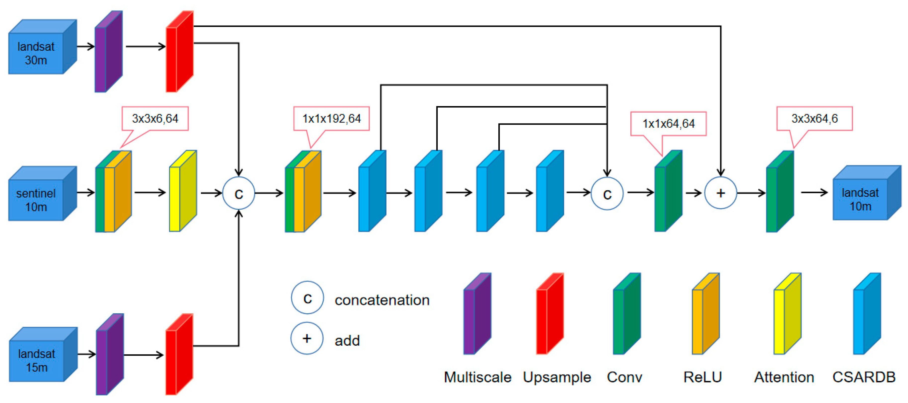
In the MARSTFN network, we divide the input data into two: auxiliary data and target reference data. The auxiliary data consist of Sentinel-2 10 m resolution bands (B02–B04, B8A, B11–B12) and the Landsat 8 15 m resolution panchromatic band. The target reference data are the Landsat 8 30 m resolution bands (b2–b7), and the final output data are the Landsat 8 10 m resolution bands (b2–b7). As depicted in Figure 1, in the branches of Landsat 8 30 m resolution bands and the 15 m resolution panchromatic band, the image undergoes feature extraction through a multiscale mechanism. Then, bicubic interpolation is applied. For the Sentinel-2 10 m resolution bands, the image features are extracted using a regular convolutional layer with 64 filters of size 3 × 3 × 6. An attention module SE is then used for further feature extraction. Subsequently, the outputs of the three branches are concatenated using a convolutional layer with 64 filters of size 1 × 1 × 192. Four CSARDB blocks with skip connections are applied to fully utilize features at different levels. Afterward, the results of all skip connections are received by a convolutional layer with 64 filters of size 1 × 1 × 64. Finally, the exported feature map is added to and convolved with the upsampled result of the coarse-resolution source (Landsat 8 30 m resolution data) using 6 filters of size 3 × 3 × 64, resulting in the final fine-resolution output (Landsat 8 10 m resolution data). In the following chapters, we will introduce the multiscale module in Section 2.1.2, the attention module in Section 2.1.3, and the CSARDB module in Section 2.1.4.

Figure 1.
The overall architecture of MARSTFN, where Multiscale represents the multiscale mechanism, Upsample represents bicubic upsampling, Conv represents convolution operation, ReLU represents the activation function, SE represents the attention mechanism, CSARDB represents the attention-coupled residual module, “c” represents concatenation operation, and “+” represents add operation.
2.1.2. Multiscale Mechanism
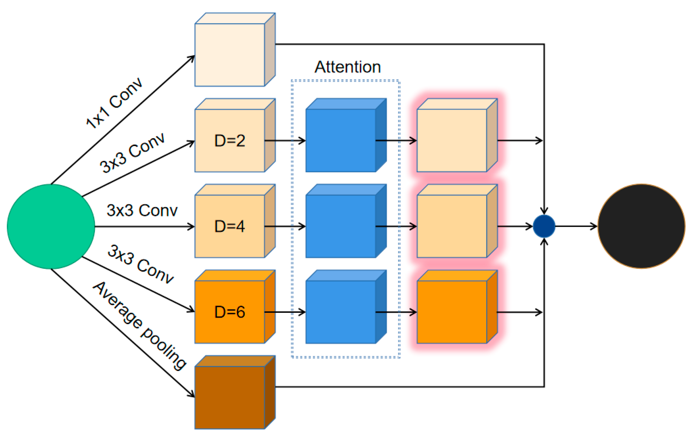
To overcome the loss of detailed information in the coarse image, we adopt a multiscale approach using convolutional kernels of varying receptive fields. This enables us to extract spatiotemporal change features and enhance fusion accuracy simultaneously. The module operates at different scales for feature extraction, as depicted in Figure 2. Firstly, at the top level, five parallel convolutional layers are expanded, including a 1 × 1 convolutional layer (Conv), three 3 × 3 convolutional layers (Conv), and an average pooling layer. Among them, the middle three 3 × 3 convolutional layers (Conv) adopt dilated convolution with dilation rates of 2, 4, and 6. This approach increases the receptive field while maintaining the feature map size and improving accuracy through multiscale effects. Subsequently, an attention module is added after each of the three dilated convolutional layers. Our attention module borrows from the DANet [45] by integrating two self-attention modules: a position attention module for spatial processing and a channel attention module for handling channel-specific data. These sub-modules harness self-attention to enhance feature fusion across the spatial and temporal dimensions. Finally, the results of each branch are fused together.
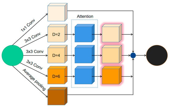
Figure 2.
Network architecture of the multiscale mechanism, where Conv represents convolution operation, Average pooling represents average pooling layer, “D” represents dilation rates, and Attention represents attention module.
2.1.3. Attention Mechanism
In consideration of the importance of fine-scale image features in the image fusion process, simple convolutional layers are insufficient for effectively extracting the spatiotemporal information from these images. Attention mechanisms have been widely applied to enhance computer vision tasks such as pan-sharpening and super-resolution. Therefore, we designed an attention module to extract feature information from fine-scale images, inspired by the Squeeze-and-Excitation Networks (SENet [46]). The network structure is shown in Figure 3, and given input with c1 feature channels, a series of convolutions and other transformations result in c2 feature channels. Unlike traditional CNNs, this is followed by three operations to re-calibrate the previously obtained features: squeeze, excitation, and scale. In the squeeze step, the feature map is compressed from height and width dimensions (h ×w × c2) to a 1 × 1 × c2 tensor via global average pooling, capturing contextual information across the entire image. Next, in the excitation step, a multilayer perceptron (MLP) models the feature channels, introducing weight parameters denoted as w. These weights are obtained through dimension reduction and normalization, generating a weight representation for each feature channel. Finally, in the scale step, these weights are applied to the original features by performing a channel-wise multiplication, recalibrating the feature responses. This process strengthens the focus on important features and enhances discriminative ability. In summary, the Squeeze-and-Excitation (SE) operation models interdependencies between feature channels through global average pooling, MLP modeling, and feature recalibration. This enhances feature expression and optimizes neural network performance.

Figure 3.
Network architecture of the attention mechanism, where represents the transform operation, represents the squeeze operation, represents the excitation operation, represents the reweight operation, h and w represent the length and width of the input data, c1 represents the number of channels before conversion, and c2 represents the number of converted channels.
In Figure 3, represents the transformation operation and the expression for its input–output relationship can be defined as follows:
where x represents the first 3D matrix on the left side of Figure 3, which is the input, u represents the second 3D matrix, which is the output, represents the c-th 2D matrix in u, represents the s-th input, and represents the c-th convolutional kernel.
represents the squeeze operation, which can be expressed as:
represents the excitation operation, which can be expressed as:
where z represents the result of the previous squeeze operation, and are the two parameters used for dimension reduction and dimension increment, respectively, represents the ReLU function, and represents the sigmoid function.
represents the reweight operation, which can be expressed as:
where s represents the result of the previous excitation operation, and represents each value in the matrix multiplied by .
2.1.4. Channel and Spatial Attention-Coupled Residual Dense Block (CSARDB) Module
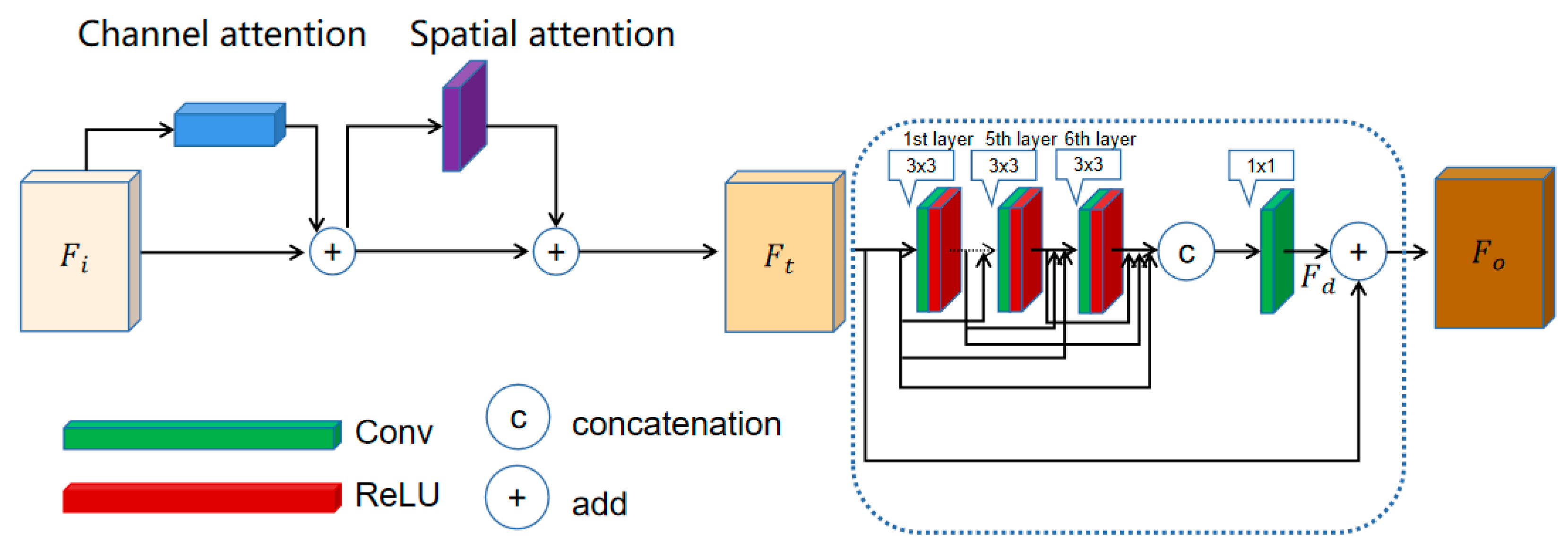
To fully represent the mapping relationship between data, we designed a complex network structure called the channel and spatial attention-coupled residual dense block. In this module, we combine the attention mechanism and the residual mechanism to form a basic unit of the network. Figure 4 visually demonstrates the enhancement made to the SENet-based Convolutional Block Attention Module (CBAM). On the left-hand side, there is a modified CBAM that includes both a channel attention module derived from the Squeeze-and-Excitation Network (SENet) and a spatial attention module emulating SENet’s functionality through global average pooling applied along the channel axis to generate a two-dimensional spatial attention coefficient matrix. The CBAM performs hybrid pooling of global average pooling and global maximum pooling on both space and channel, enabling the extraction of more effective information. The output feature map is then fed into the right side’s residual dense block (RDB), which utilizes both residual learning and dense connections. The block consists of six “Conv + ReLU” layers, each containing a 3 × 3 ordinary convolutional layer (Conv) and an activation function unit (ReLU). Additionally, the feature maps from all previous layers are fed into each layer via skip connections, enhancing feature propagation and greatly improving the network feature reuse ability. In the skip connections, the output expression of each “Conv + ReLU” layer (1 ≤ n ≤ 6) can be expressed as:
where represents the feature map output from the attention mechanism, “concat” denotes the concatenation operation, , … represents the feature maps of the first layer to the (n − 1)-th layer, and represents the feature map of the n-th layer. The final output of the CSARDB block is represented as:
where represents the residual feature maps obtained through skip connections from the previous six layers.
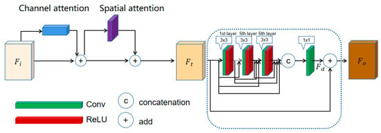
Figure 4.
Network architecture of the CSARDB module, Conv represents convolution operation, ReLu represents the activation function, “c” represents concatenation operation, and “+” represents add operation.
2.2. Loss Function
To quantify the discrepancy between the predicted results of the model and the actual observations, a loss function is employed. Within the context of this network, the loss function is structured as follows:
where L1 represents the L1-norm term used to constrain the error between predictions and labels, Lf represents the Frobenius norm term, and a and b are adaptive parameters, and they can be expressed as:
3. Experiment Results
3.1. Datasets and Network Training
The experimental data in this study were obtained from the two benchmark datasets provided in [40]. These datasets were chosen due to their diverse characteristics, including varying degrees of spatial heterogeneity and temporal dynamics. By utilizing such datasets, we can assess the feasibility and effectiveness of the proposed method in handling complex and changing environmental conditions. The datasets consist of two study areas. The first one is located in Hailar, Northeast China [40], situated at the western foot of the Daxing’anling Mountains, where it intersects with the low hills and high plains of Hulunbuir. The terrain types in this area include low hills, high plains, low flatlands, and riverbanks. The second study area is located in Dezhou, Shandong Province [40], which is a floodplain of the Yellow River characterized by a higher southwest and a lower northeast topography. The general landforms can be classified into the three following categories: highlands, slopes, and depressions. The climate is warm temperate continental monsoon, with four distinct seasons and obvious dry and wet periods. The Hailar dataset includes 23 scenes covering the entire year of 2019, while the Dezhou dataset includes 24 scenes for the year 2018. Both datasets underwent preprocessing steps including geometric calibration and spatial cropping [47] to ensure consistent image sizes. The size of the Hailar images is 3960 × 3960, and the size of the Dezhou images is 2970 × 2970. To ensure robustness in the model development process, each dataset was partitioned into three distinct subsets—training, validation, and testing. Specifically, 60%, 20%, and 20% of the data were allocated for training, validation, and testing purposes, respectively. The purpose of the validation set was to find the optimal network parameters to ensure the best performance. Each dataset consists of four types of images, including Landsat 8 (30 m, 15 m, and 10 m) and Sentinel-2 (10 m) data. In addition, we used Sentinel-2 10 m resolution images of the reference date in the input data as the ground truth images for comparison with the experimental results.
3.2. Evaluation Indicators
Under the same experimental conditions, we compared our model with the following four models: FSDAF [26], STARFM-SI [23], ATPRK [29], and DSTFN [40]. FSDAF fuses images through spatial interpolation and unmixing. STARFM-SI is a simplified version of STARFM that fuses images through weighted averaging under simplified input conditions. ATPRK is a geostatistical fusion method involving the modeling of semivariogram matrices. DSTFN predicts images by incorporating a degradation constraint term.
The Structural Similarity Index (SSIM) [48], Peak Signal-to-Noise Ratio (PSNR) [49], and Root Mean Square Error (RMSE) [50] are employed to give a quantitative evaluation. SSIM serves as an indicator for assessing the visual similarity between two given images. The expression for SSIM can be defined as:
where and represent the mean values of the predicted image x and the ground truth image y, respectively. and represent the variances of the predicted image x and the ground truth image y, respectively. represents the covariance between the predicted image x and the ground truth image y. and are constants to avoid division by zero and prevent potential system errors. The SSIM score falls within the range of −1 to 1 and higher values denote lesser discrepancies between the predicted and ground truth images, signifying better similarity.
PSNR is used to evaluate the quality of the images. The PSNR value is commonly used as a reference for measuring image quality, but it has limitations as it only measures the quality between the maximum signal value and background noise. The PSNR is measured in decibels (dB) and can be obtained using Mean Squared Error (MSE), which is expressed as:
where m and n represent the height and width of the images, x represents the predicted image, and y represents the ground truth image. The PSNR is expressed as:
where represents the maximum pixel value of the ground truth image. A higher PSNR value signifies lower image distortion, implying that the predicted image is in closer proximity to the ground truth image.
RMSE serves as a measure of deviation between the predicted image and the ground truth image. It is derived from the Square Mean Error (MSE), but due to its square root operation, it is more responsive to fluctuations in data than MSE. As such, RMSE offers a more comprehensive depiction of the differences between the images. Lower RMSE values indicate a reduced image deviation, denoting enhanced proximity between the predicted and ground truth images. The expression for RMSE can be defined as:
3.3. Parameter Setting
We employed three machine learning-based methodologies, including FSDAF [28], STARFM-SI [25], and ATPRK [31], without requiring any prior training stages. Instead, these approaches were subjected to testing using a 20% validation dataset. Conversely, the deep learning-based models DSTFN [40] and MARSTFN underwent extensive training sessions. For this purpose, we utilized a high-performance server environment, equipped with an 8-core CPU and a powerful Tesla T4 GPU, to facilitate efficient model optimization. Throughout the training process, we maintained a consistent learning rate of 0.001, and utilized a batch size of 64 samples, executing 100 training epochs to ensure optimal model convergence.
3.4. Results
3.4.1. Evaluation of the Methods on the Hailar Dataset
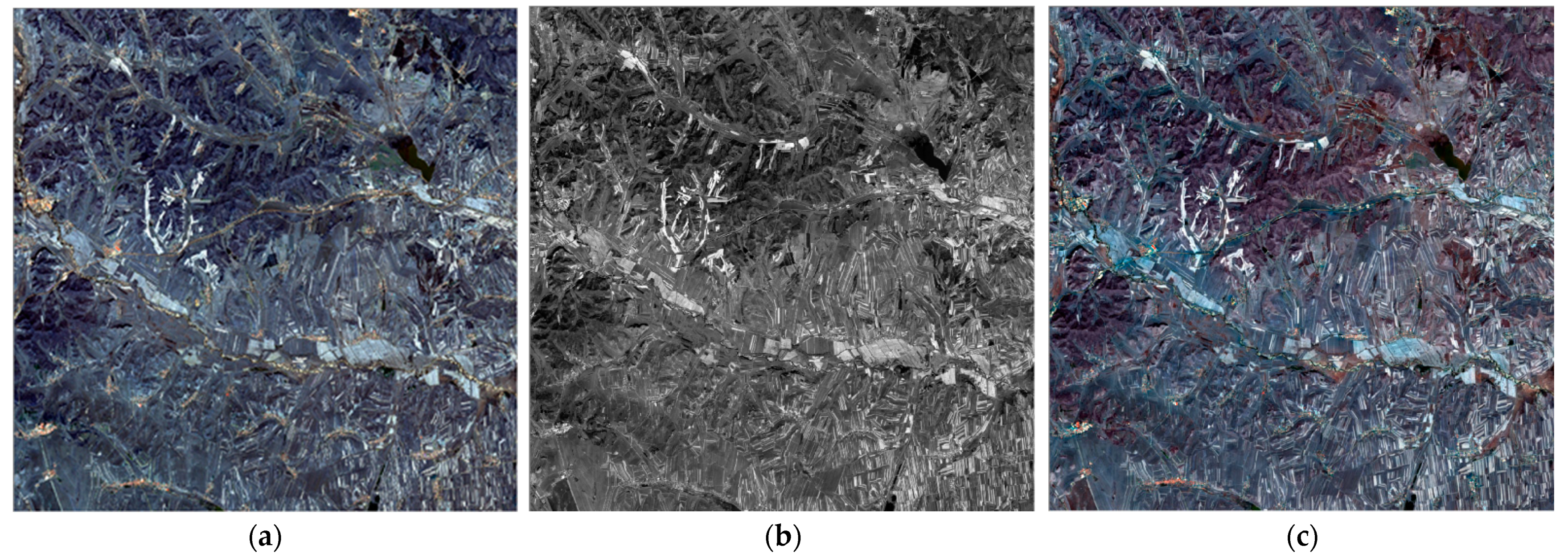
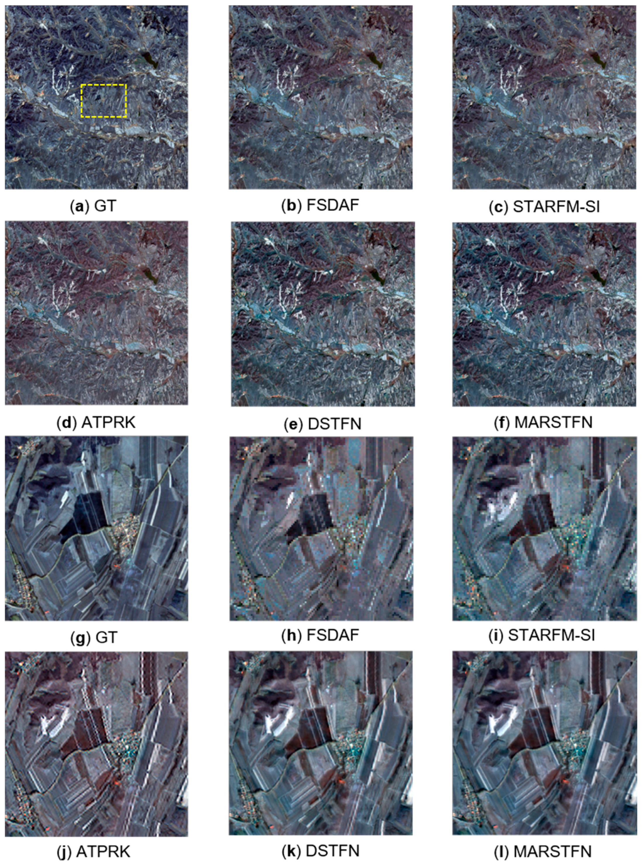
Figure 5 presents a set of input data on the Hailar dataset, where (a) and (b) represent auxiliary data, namely Sentinel-2 10 m resolution data on 19 October 2019, and Landsat 8 15 m resolution data on 22 October 2019, respectively. Panel (c) represents the target reference data, which are Landsat 8 30 m resolution data on 22 October 2019. Figure 6 displays the prediction results of various methods on the Hailar dataset. “GT” represents the reference image, which is the ground truth image. Panels (a) to (f) show the prediction results of various methods on 22 October 2019, for Landsat 8 data with a resolution of 10 m. Panels (g) to (l) show magnified views of a subset region (marked with a yellow square) of panels (a) to (f), respectively. As shown in Figure 6, all fusion methods can predict spatial details of the images well. The phenology change in the Hailar region is relatively slow, resulting in good overall prediction performance. However, the fusion results of each method differ. Panels (a) to (f) show that DSTFN and MARSTFN perform better in restoring spectral information, while the recovery effects of the other three methods are slightly lacking, especially ATPRK, which shows more distortion in spectral recovery. Moreover, for panels (g) to (l), the differences in fusion results are more pronounced. The fusion results of FSDAF and STARFM-SI have more obvious distortion, and the image edges are relatively blurred, losing many spatial texture details. The fusion results obtained by ATPRK exhibit a slight improvement compared to the first two methods but still have some distortion and large errors compared to the original image. Although the fusion effect of DSTFN is better than the previous methods, with less image distortion and better recovery of texture details, the spectral recovery is slightly lacking in detail. Our proposed MARSTFN performs well in reducing distortion, maintaining good texture details, and restoring spectral information. The results above indicate that our proposed MARSTFN has better fusion results compared to the other methods on the Hailar dataset, not only predicting texture details but also handling spectral information well.
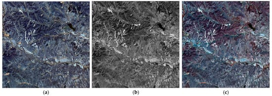
Figure 5.
Input data of the Hailar dataset.
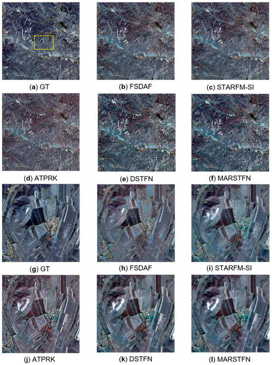
Figure 6.
(g–l) provide detailed views of the Hailar dataset’s subset region highlighted by a yellow square in (a–f).
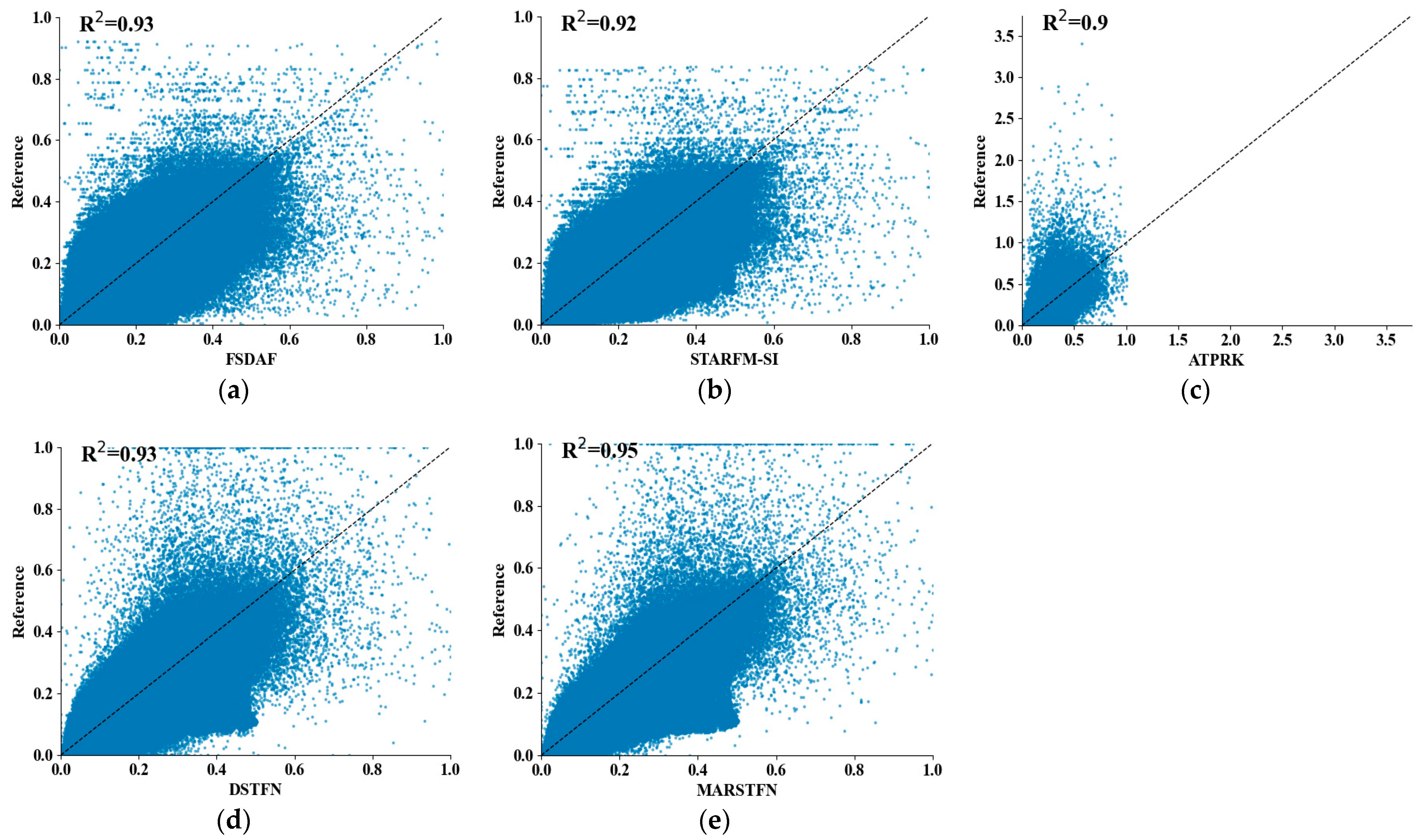
Figure 7 presents the correlation between various fusion results and the real image on the Hailar dataset. The samples are derived from the scene images shown in Figure 6. In this figure, we utilize the coefficient to represent the prediction results. is a statistical measure of the degree of fit between the data and the regression function. It is defined by the following formula:
where represents the observed value of the i-th pixel denotes the predicted value, is the mean value, and n is the number of pixels. The value of typically falls within the range of 0 to 1, with a value closer to 1 indicating better prediction performance.
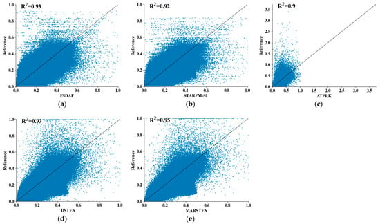
Figure 7.
(a–e) represent the correlation between the predicted images of each fusion method and the real images, and represents the statistical measure of the degree of fit between the data and the regression function.
It can be observed that the FSDAF, STARFM-SI, and ATPRK methods exhibit relatively poor correlation with the real image. On the other hand, MARSTFN demonstrates a slightly higher -value compared to DSTFN, and there are fewer points deviating from the real values. Therefore, both the statistical measurement of function fitting and visual assessment suggest that the predicted results of MARSTFN are closer to the real image compared to the other four methods.
3.4.2. Evaluation of the Methods on the Dezhou Dataset
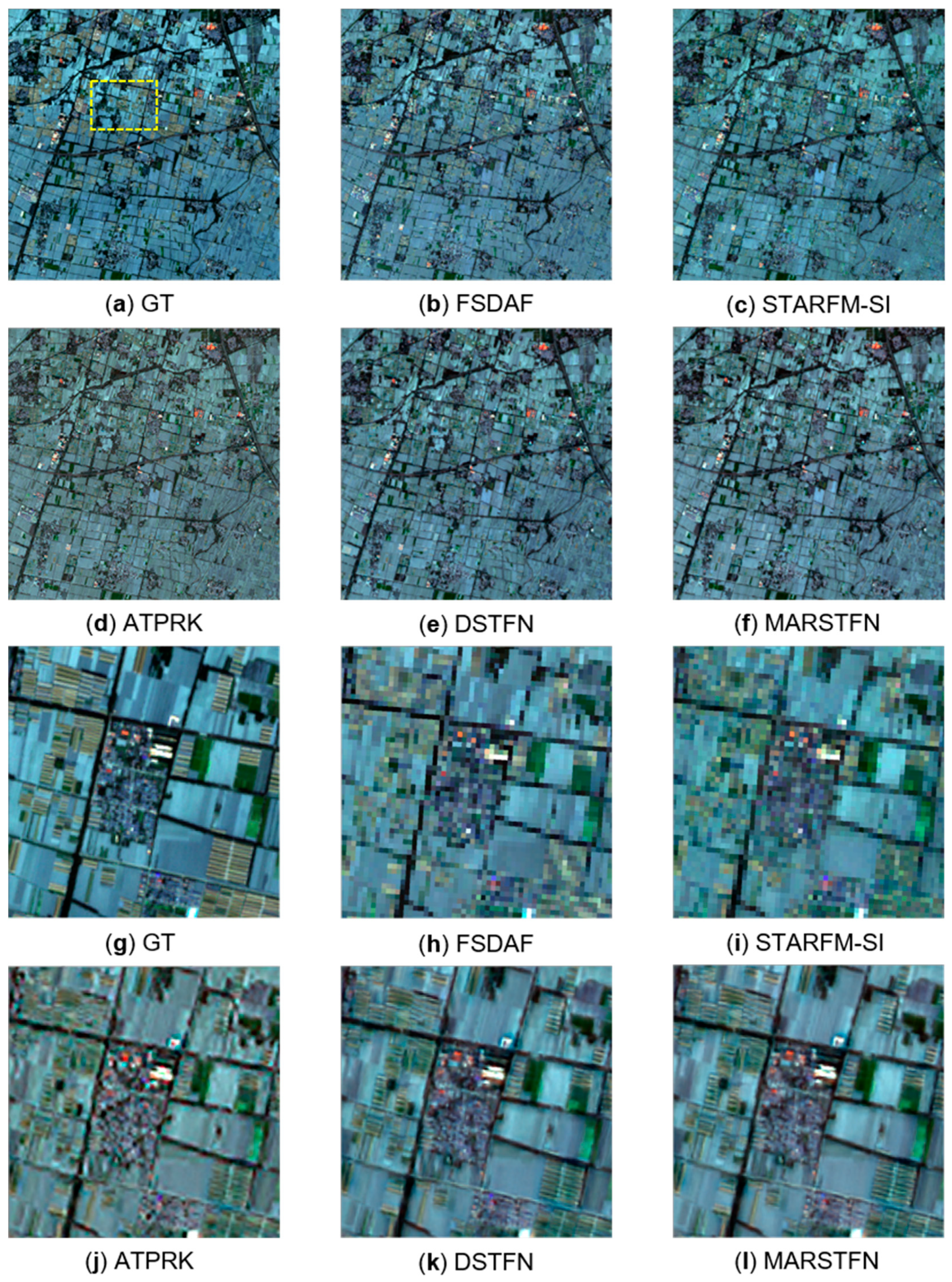
Figure 8 shows a set of input data on the Dezhou dataset, where (a) and (b) represent auxiliary data, namely Sentinel-2 10 m resolution data on 17 October 2018, and Landsat 8 15 m resolution data on 26 October 2018, respectively. Panel (c) represents the target reference data, which are Landsat 8 30 m resolution data on 26 October 2018. Figure 9 displays the prediction results of the various methods on the Dezhou dataset. “GT” represents the reference image, which is the ground truth image. Panels (a) to (f) show the prediction results of these five methods on 26 October 2018, for Landsat 8 data with a resolution of 10 m. Panels (g) to (l) show magnified views of a subset region (marked with a yellow square) of panels (a) to (f), respectively. As shown in Figure 9, it can be observed that all fusion methods can to some extent improve the accuracy of the predicted images, indicating that these methods possess the ability to recover temporal and spatial changes in the images. However, the fusion results of different methods vary. From (a) to (f), it can be observed that STARFM-SI and MARSTFN perform relatively well in terms of spectral recovery, while the spectral recovery effect of the other three methods is relatively poor. Furthermore, for (g) to (l), the differences in the fusion results of these methods are more pronounced. From the images, it can be observed that the fusion results of FSDAF and STARFM-SI are very buried, exhibiting significant distortion and loss of texture detail. Although the fusion result of ATPRK is slightly better compared to the first two methods, it still exhibits some distortion and has a larger error compared to the original image. While the fusion result of DSTFN exhibits fewer distortions and relatively better preservation of spatial details, the spectral recovery effect is still lacking. Our proposed MARSTFN method processes the feature information of the image well. Although it does not perfectly restore the real image, it exhibits smaller color differences compared to the other methods and preserves spatial texture details relatively well. Our research findings conclusively demonstrate that, across all evaluations conducted on the Dezhou dataset, the proposed MARSTFN method demonstrates a clear advantage over competing strategies in terms of overall performance. Specifically, the resulting fused image produced by our method exhibits a higher degree of similarity to the corresponding ground truth image relative to alternative techniques.
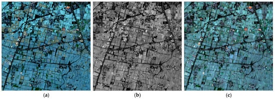
Figure 8.
Input data of the Dezhou dataset.
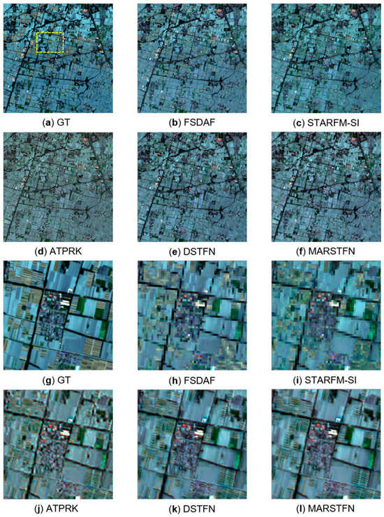
Figure 9.
(g–l) provide detailed views of the Dezhou dataset’s subset region highlighted by a yellow square in (a–f).
Figure 10 shows the correlation between various fusion methods and the real image on the Dezhou dataset, with samples taken from the scene graph in Figure 9. It can be observed that the ATPRK method has the poorest prediction performance, which may be attributed to its status as a geostatistical method for data fusion, leading to poor performance in areas with fast phenological changes. In contrast, the MARSTFN method exhibits the highest correlation with the real image compared to the other four methods, indicating superior performance. Based on the above analysis, in areas with significant spectral variations, the predictive performance of MARSTFN remains closer to the real image compared to the other four methods.
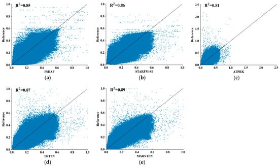
Figure 10.
(a–e) represent the correlation between the predicted image of each fusion method and the real image, and represents the statistical measure of the degree of fit between the data and the regression function.
3.4.3. Quantitative Evaluation
We performed a total of six trials on the Hailar dataset, and Table 2 presents the quantitative assessment results of all fusion methodologies tested on this set. Highlighted in bold are the optimal values for each assessment metric. As illustrated in the table, our proposed method outperforms FSDAF and STARFM-SI by approximately 4.5% and 4.6% in terms of PSNR, respectively. ATPRK performs the worst, while DSTFN demonstrates better fusion results than the previous three methods, indicating its ability to recover image texture details effectively. In terms of SSIM, ATPRK outperforms FSDAF and STARFM-SI, possibly because the phenological changes in the Hailar dataset are relatively slow, allowing ATPRK to make better image predictions. MARSTFN achieves the best performance, indicating its ability to recover spectral information well in areas with slow geological variations. Regarding RMSE, MARSTFN reduces the RMSE values by 15% and 19% compared to FSDAF and ATPRK, respectively. However, STARFM-SI performs worse than DSTFN, possibly due to its simplicity as a machine learning method that only considers partial pixel reconstruction, making it less suitable for predicting larger spatial regions. For the FSDAF, STARFM-SI, and ATPRK algorithms, the experimental results on certain dates are slightly better than those of DSTFN, possibly because the former three algorithms are based on physical models, which can exhibit good prediction performance in areas with slow geological structural changes. Additionally, the instability of the DSTFN model can lead to unpredictable accuracy fluctuations. These experimental results demonstrate that the MARSTFN method achieves the best results across all metrics. We executed a total of five trials on the Dezhou dataset, and Table 3 compiles the quantitative assessment outcomes of all fusion methodologies tested on this set. Highlighted in bold are the optimal values for each assessment metric. As shown in the table, our proposed MARSTFN model demonstrates improved fusion results compared to other algorithms across the evaluation metrics. For instance, in terms of PSNR, our method outperforms the machine learning-based FSDAF and STARFM-SI methods by approximately 7% and 5.8%, respectively, and achieves an improvement of about 2.1% compared to the deep learning-based DSTFN method. On the other hand, ATPRK exhibits the poorest quantitative evaluation results, possibly due to its limited flexibility in preserving the spectral distribution of the original images as a geostatistical data fusion method. In terms of the Structural Similarity Index (SSIM), both FSDAF and ATPRK show the worst fusion results, while our proposed method achieves approximately 0.9% and 1.1% improvements over these two methods, respectively. The enhancement in STARFM-SI, which incorporates auxiliary data, leads to better fusion results compared to the original STARFM method. Furthermore, MARSTFN, with the introduction of a multiscale mechanism and attention mechanism, is able to better capture the information of the images compared to DSTFN. From the table, it can be observed that FSDAF and ATPRK demonstrate the poorest prediction performance, with our proposed method reducing the error values by approximately 20.2% and 27.4%, respectively. The RMSE value of STARFM-SI is worse than that of the DSTFN method, indicating the ability of DSTFN to predict spectral information effectively. The marginal improvement in performance observed for FSDAF, STARFM-SI, and ATPRK algorithms compared to DSTFN on specific dates may be indicative of DSTFN’s limited suitability for regions with complex and rapidly changing ground features, highlighting the need for enhanced stability. MARSTFN outperforms the other methods across all three metrics, demonstrating its effectiveness in recovering spectral information in regions with significant spectral variations. Therefore, the experimental results indicate that introducing a multiscale mechanism, attention mechanism, and residual mechanism in our network can improve the accuracy of predicted images and effectively fuse the images.

Table 2.
Quantitative evaluation of various methods on the Hailar dataset. The best values of the index are marked in bold.

Table 3.
Quantitative evaluation of various methods on the Dezhou dataset. The best values of the index are marked in bold.
4. Discussion
4.1. Generalized Analysis
The experimental outcomes concerning the Hailar dataset exhibit the superior performance of our method in comparison to rival techniques, achieving notable gains in fusion image accuracy through the integration of the multiscale mechanism, attention mechanism, and residual network. Subjective assessments reveal that fusion results from FSDAF and STARFM-SI methods are marred by pronounced distortions, whereas our method consistently generates images that closely resemble their associated ground truth counterparts. This observation suggests that our approach is adept at predicting images in scenarios characterized by sluggish phenological transformations. Furthermore, the outcomes derived from the Dezhou dataset showcase the ability of our method to accurately represent spatiotemporal characteristics and spectral variances embedded in images of regions exhibiting substantial phenological fluctuations. This accomplishment is attributed to the enhanced capability of our approach to effectively extract image features and preserve intricate details through a distinctive fusion strategy. Our proposed method, MARSTFN, achieves the following results: (1) It utilizes a multiscale mechanism to extract features from coarse images, incorporating dilated convolutions in the multiscale mechanism. (2) It employs an attention mechanism to extract features from fine images, preserving spectral information to the maximum extent. (3) It introduces the CSARDB module, which combines the attention mechanism and residual network. The CSARDB module fuses the features extracted from the coarse images processed by the multiscale mechanism and the fine images processed by the attention mechanism. Through skip connections, it continuously extracts features, maximizing feature extraction and thus achieving more accurate prediction results.
Figure 11 shows the 10 m images generated by MARSTFN, as well as the comparison between 10 m and 30 m in four different scenes. We selected four representative areas with diverse geological landscapes, including farmland and urban buildings, and zoomed in to compare the scenes at 10 m and 30 m resolutions. It can be observed that the original 30 m image fails to provide sufficient spatial information, whereas the 10 m image significantly improves the spatial resolution, enabling better recognition of geospatial structures and enhanced object identification capabilities. Therefore, our proposed MARSTFN deep network, which incorporates multiscale mechanisms, attention mechanisms, and residual networks, effectively predicts medium- to high-resolution images.
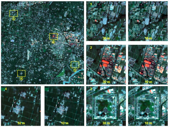
Figure 11.
Imagery of 10 m resolution generated by MARSTFN and a comparison between scenes with 30 m and 10 m resolution.
4.2. Ablation Experiments
To substantiate the significance of the multiscale mechanism, attention mechanism, and residual network modules, we devised three separate experiments. For experiment 1, the multiscale mechanism was eliminated while maintaining the attention mechanism and residual network. In experiment 2, the attention mechanism was discarded but the multiscale mechanism and residual network remained intact. Lastly, in experiment 3, the residual network was eradicated but the multiscale mechanism and attention mechanism were retained. Table 4 presents the experimental results for these three experiments, where “ARNet” represents the network structure without the multiscale mechanism, “MRNet” represents the network structure without the attention mechanism, and “MANet” represents the network structure without the residual network. The best values for the evaluation metrics are highlighted in bold.

Table 4.
The quantitative evaluation of ablation experiments. The best values of the index are marked in bold.
From Table 4, it can be seen that on the Hailar dataset, both MRNet and MANet have higher SSIM values than ARNet, indicating that these two models have better spatial information prediction capabilities than ARNet. Additionally, the RMSE values for MRNet and MANet are lower than those for ARNet, indicating that these two models have more accurate spectral information change predictions than ARNet. This suggests that incorporating a multiscale mechanism can enhance the model’s prediction ability, and combining the multiscale mechanism with either an attention mechanism or a residual network can effectively predict both spatial and spectral information in the image. On the Dezhou dataset, the SSIM value for ARNet is higher than that for MRNet, indicating that the combination of the attention mechanism and residual network has achieved good results. Moreover, the SSIM value for MANet is also higher than that for MRNet, indicating that adding an attention mechanism can improve the model’s prediction ability, and introducing a residual network on this basis can further enhance the model’s ability to predict high-resolution images. On both the Hailar and Dezhou datasets, MARSTFN achieves optimal SSIM and RMSE values, indicating that incorporating a multiscale mechanism, an attention mechanism, and a residual network enables the effective extraction of both spatial and spectral information from the image. Figure 12 shows the results of the three comparison experiments on 8 February 2019 on the Hailar dataset, and Figure 13 displays the results of the three comparison experiments on 26 October 2018 on the Dezhou dataset.

Figure 12.
The comparative experimental methods’ results on the Hailar dataset.

Figure 13.
The comparative experimental methods’ results on the Dezhou dataset.
In Figure 12 and Figure 13, (a) represents the real image, (b) represents the prediction result of ARNet, (c) represents MRNet’s prediction result, (d) represents MANet’s prediction result, and (e) represents MARSTFN’s prediction result. From Figure 12, it can be observed that the prediction result of ARNet exhibits significant spectral distortion, while the prediction results of MRNet, MANet, and MARSTFN closely resemble the real image. This indicates that the introduction of a multiscale mechanism can effectively capture spatial and spectral details of the image, which also corresponds to the quantitative evaluation results. From Figure 13, it can be observed that the prediction results of MRNet and MANet have lost a considerable amount of texture details. In comparison, ARNet maintains texture details relatively well. This suggests that the introduction of an attention mechanism is crucial for recovering texture details in areas with significant spectral variations. In both Figure 12 and Figure 13, the prediction results of MARSTFN are the closest to the real image, indicating that our approach can effectively extract image features. Although our approach has made improvements in extracting spatial and spectral information from the images, there are still some shortcomings, such as the relatively low prediction accuracy in areas with significant spectral variations, which may be addressed by collecting more suitable datasets in the future.
5. Conclusions
We validated the effectiveness of our proposed spatiotemporal fusion network (MARSTFN) using two datasets and obtained the best experimental results. The main contributions of our research are summarized as follows:
- We introduced a novel spatiotemporal fusion (STF) architecture, namely MARSTFN, which combines a multiscale mechanism, an attention mechanism, and a residual network to effectively extract spatial and spectral information from the images.
- Through comprehensive experiments on two datasets, we demonstrated that MARSTFN outperforms other existing methods in terms of image detail preservation, as well as overall prediction accuracy.
- Our proposed STF architecture addresses the limitations of existing methods in capturing both spatial and spectral information, particularly in areas with significant spectral variations.
The experimental outcomes confirm the proficiency of our proposed methodology in accurately forecasting images across various scenarios. This includes the Hailar region, characterized by gradual phenological transformations, and the Dezhou area, featuring swift phenological alterations. Our approach, harnessing Sentinel-2 10 m resolution data and Landsat 8 15 m resolution data as supplementary resources, successfully upgrades the Landsat 30 m resolution data to a 10 m resolution through the integration of the multiscale mechanism, attention mechanism, and residual network. This fusion framework skillfully harmonizes the intricate details present in low-resolution imagery with the thorough spatial characteristics of high-resolution data, thereby optimizing the production of highly accurate high-spatial high-temporal resolution predictions. Nevertheless, access to comprehensive and relevant datasets remains a limiting factor in significantly enhancing the overall prediction accuracy. As such, we plan to dedicate further research efforts toward identifying and utilizing more appropriate and extensive datasets for spatiotemporal fusion purposes. These issues can be further discussed in future studies.
Author Contributions
Conceptualization, Q.C.; data curation, R.X. and J.W.; formal analysis, Q.C.; funding acquisition, Q.C.; methodology, Q.C., R.X. and F.Y.; validation, R.X.; visualization, R.X.; writing—original draft, R.X.; writing—review and editing, Q.C., J.W. and F.Y. All authors have read and agreed to the published version of the manuscript.
Funding
This research was funded by the National Natural Science Foundation of China (grant number 42171383), the Fundamental Research Funds for the Central Universities, China University of Geosciences (Wuhan) (No.CUG2106212) and Open Research Project of The Hubei Key Laboratory of Intelligent Geo-Information Processing under Grant KLIGIP-2023-B04.
Data Availability Statement
The data presented in this study are available upon request from the corresponding author.
Conflicts of Interest
The authors declare no conflicts of interest.
References
- Gutman, G.; Byrnes, R.A.; Masek, J.; Covington, S.; Justice, C.; Franks, S.; Headley, R. Towards monitoring land-cover and land-use changes at a global scale: The Global Land Survey 2005. Photogramm. Eng. Remote Sens. 2008, 74, 6–10. [Google Scholar]
- Woodcock, C.E.; Allen, R.; Anderson, M.; Belward, A.; Bindschadler, R.; Cohen, W.; Gao, F.; Goward, S.N.; Helder, D.; Helmer, E. Free Access to Landsat Imagery. Science 2008, 320, 1011. [Google Scholar] [CrossRef] [PubMed]
- Roy, D.P.; Wulder, M.A.; Loveland, T.R.; Woodcock, C.E.; Allen, R.G.; Anderson, M.C.; Helder, D.; Irons, J.R.; Johnson, D.M.; Kennedy, R. Landsat-8: Science and product vision for terrestrial global change research. Remote Sens. Environ. 2014, 145, 154–172. [Google Scholar] [CrossRef]
- Justice, C.O.; Vermote, E.; Townshend, J.R.; Defries, R.; Roy, D.P.; Hall, D.K.; Salomonson, V.V.; Privette, J.L.; Riggs, G.; Strahler, A. The Moderate Resolution Imaging Spectroradiometer (MODIS): Land remote sensing for global change research. IEEE Trans. Geosci. Remote Sens. 1998, 36, 1228–1249. [Google Scholar] [CrossRef]
- Xu, Y.; Huang, B.; Xu, Y.; Cao, K.; Guo, C.; Meng, D. Spatial and temporal image fusion via regularized spatial unmixing. IEEE Geosci. Remote Sens. Lett. 2015, 12, 1362–1366. [Google Scholar]
- Kim, D.-H.; Sexton, J.O.; Noojipady, P.; Huang, C.; Anand, A.; Channan, S.; Feng, M.; Townshend, J.R. Global, Landsat-based forest-cover change from 1990 to 2000. Remote Sens. Environ. 2014, 155, 178–193. [Google Scholar] [CrossRef]
- Senf, C.; Pflugmacher, D.; Heurich, M.; Krueger, T. A Bayesian hierarchical model for estimating spatial and temporal variation in vegetation phenology from Landsat time series. Remote Sens. Environ. 2017, 194, 155–160. [Google Scholar] [CrossRef]
- Fu, P.; Weng, Q. A time series analysis of urbanization induced land use and land cover change and its impact on land surface temperature with Landsat imagery. Remote Sens. Environ. 2016, 175, 205–214. [Google Scholar] [CrossRef]
- Claverie, M.; Masek, J.G.; Ju, J.; Dungan, J.L. Harmonized Landsat-8 Sentinel-2 (HLS) Product User’s Guide; National Aeronautics and Space Administration (NASA): Washington, DC, USA, 2017.
- Skakun, S.; Kussul, N.; Shelestov, A.; Kussul, O. Flood hazard and flood risk assessment using a time series of satellite images: A case study in Namibia. Risk Anal. 2014, 34, 1521–1537. [Google Scholar] [CrossRef]
- Melaas, E.K.; Friedl, M.A.; Zhu, Z. Detecting interannual variation in deciduous broadleaf forest phenology using Landsat TM/ETM+ data. Remote Sens. Environ. 2013, 132, 176–185. [Google Scholar] [CrossRef]
- White, J.C.; Wulder, M.A.; Hermosilla, T.; Coops, N.C.; Hobart, G.W. A nationwide annual characterization of 25 years of forest disturbance and recovery for Canada using Landsat time series. Remote Sens. Environ. 2017, 194, 303–321. [Google Scholar] [CrossRef]
- Drusch, M.; Del Bello, U.; Carlier, S.; Colin, O.; Fernandez, V.; Gascon, F.; Hoersch, B.; Isola, C.; Laberinti, P.; Martimort, P. Sentinel-2: ESA’s optical high-resolution mission for GMES operational services. Remote Sens. Environ. 2012, 120, 25–36. [Google Scholar] [CrossRef]
- Brown, C.F.; Brumby, S.P.; Guzder-Williams, B.; Birch, T.; Hyde, S.B.; Mazzariello, J.; Czerwinski, W.; Pasquarella, V.J.; Haertel, R.; Ilyushchenko, S. Dynamic World, Near real-time global 10 m land use land cover mapping. Sci. Data 2022, 9, 251. [Google Scholar] [CrossRef]
- Gao, F.; Zhang, X. Mapping crop phenology in near real-time using satellite remote sensing: Challenges and opportunities. J. Remote Sens. 2021, 2021, 8379391. [Google Scholar] [CrossRef]
- Soltanikazemi, M.; Minaei, S.; Shafizadeh-Moghadam, H.; Mahdavian, A. Field-scale estimation of sugarcane leaf nitrogen content using vegetation indices and spectral bands of Sentinel-2: Application of random forest and support vector regression. Comput. Electron. Agric. 2022, 200, 107130. [Google Scholar] [CrossRef]
- Putri, A.F.S.; Widyatmanti, W.; Umarhadi, D.A. Sentinel-1 and Sentinel-2 data fusion to distinguish building damage level of the 2018 Lombok Earthquake. Remote Sens. Appl. Soc. Environ. 2022, 26, 100724. [Google Scholar]
- Ju, J.; Roy, D.P. The availability of cloud-free Landsat ETM+ data over the conterminous United States and globally. Remote Sens. Environ. 2008, 112, 1196–1211. [Google Scholar] [CrossRef]
- Shen, H.; Wu, J.; Cheng, Q.; Aihemaiti, M.; Zhang, C.; Li, Z. A spatiotemporal fusion based cloud removal method for remote sensing images with land cover changes. IEEE J. Sel. Top. Appl. Earth Obs. Remote Sens. 2019, 12, 862–874. [Google Scholar] [CrossRef]
- Pan, L.; Xia, H.; Yang, J.; Niu, W.; Wang, R.; Song, H.; Guo, Y.; Qin, Y. Mapping cropping intensity in Huaihe basin using phenology algorithm, all Sentinel-2 and Landsat images in Google Earth Engine. Int. J. Appl. Earth Obs. Geoinf. 2021, 102, 102376. [Google Scholar] [CrossRef]
- Gao, F.; Masek, J.; Schwaller, M.; Hall, F. On the blending of the Landsat and MODIS surface reflectance: Predicting daily Landsat surface reflectance. IEEE Trans. Geosci. Remote Sens. 2006, 44, 2207–2218. [Google Scholar]
- Zhu, X.; Chen, J.; Gao, F.; Chen, X.; Masek, J.G. An enhanced spatial and temporal adaptive reflectance fusion model for complex heterogeneous regions. Remote Sens. Environ. 2010, 114, 2610–2623. [Google Scholar] [CrossRef]
- Wu, J.; Cheng, Q.; Li, H.; Li, S.; Guan, X.; Shen, H. Spatiotemporal fusion with only two remote sensing images as input. IEEE J. Sel. Top. Appl. Earth Obs. Remote Sens. 2020, 13, 6206–6219. [Google Scholar] [CrossRef]
- Zhukov, B.; Oertel, D.; Lanzl, F.; Reinhackel, G. Unmixing-based multisensor multiresolution image fusion. IEEE Trans. Geosci. Remote Sens. 1999, 37, 1212–1226. [Google Scholar] [CrossRef]
- Wu, M.; Niu, Z.; Wang, C.; Wu, C.; Wang, L. Use of MODIS and Landsat time series data to generate high-resolution temporal synthetic Landsat data using a spatial and temporal reflectance fusion model. J. Appl. Remote Sens. 2012, 6, 063507. [Google Scholar]
- Zhu, X.; Helmer, E.H.; Gao, F.; Liu, D.; Chen, J.; Lefsky, M.A. A flexible spatiotemporal method for fusing satellite images with different resolutions. Remote Sens. Environ. 2016, 172, 165–177. [Google Scholar] [CrossRef]
- Cheng, Q.; Liu, H.; Shen, H.; Wu, P.; Zhang, L. A spatial and temporal nonlocal filter-based data fusion method. IEEE Trans. Geosci. Remote Sens. 2017, 55, 4476–4488. [Google Scholar] [CrossRef]
- Xue, J.; Leung, Y.; Fung, T. A Bayesian data fusion approach to spatio-temporal fusion of remotely sensed images. Remote Sens. 2017, 9, 1310. [Google Scholar] [CrossRef]
- Wang, Q.; Blackburn, G.A.; Onojeghuo, A.O.; Dash, J.; Zhou, L.; Zhang, Y.; Atkinson, P.M. Fusion of Landsat 8 OLI and Sentinel-2 MSI data. IEEE Trans. Geosci. Remote Sens. 2017, 55, 3885–3899. [Google Scholar] [CrossRef]
- Wei, J.; Wang, L.; Liu, P.; Chen, X.; Li, W.; Zomaya, A.Y. Spatiotemporal fusion of MODIS and Landsat-7 reflectance images via compressed sensing. IEEE Trans. Geosci. Remote Sens. 2017, 55, 7126–7139. [Google Scholar] [CrossRef]
- Wang, Z.; Fang, S.; Zhang, J. Spatiotemporal Fusion Model of Remote Sensing Images Combining Single-Band and Multi-Band Prediction. Remote Sens. 2023, 15, 4936. [Google Scholar] [CrossRef]
- Chen, G.; Lu, H.; Di, D.; Li, L.; Emam, M.; Jing, W. StfMLP: Spatiotemporal Fusion Multilayer Perceptron for Remote-Sensing Images. IEEE Geosci. Remote Sens. Lett. 2022, 20, 5000105. [Google Scholar] [CrossRef]
- Masi, G.; Cozzolino, D.; Verdoliva, L.; Scarpa, G. Pansharpening by convolutional neural networks. Remote Sens. 2016, 8, 594. [Google Scholar] [CrossRef]
- Yuan, Q.; Wei, Y.; Meng, X.; Shen, H.; Zhang, L. A multiscale and multidepth convolutional neural network for remote sensing imagery pan-sharpening. IEEE J. Sel. Top. Appl. Earth Obs. Remote Sens. 2018, 11, 978–989. [Google Scholar] [CrossRef]
- Dong, C.; Loy, C.C.; He, K.; Tang, X. Image super-resolution using deep convolutional networks. IEEE Trans. Pattern Anal. Mach. Intell. 2015, 38, 295–307. [Google Scholar] [CrossRef]
- Mishra, B.; Shahi, T.B. Deep learning-based framework for spatiotemporal data fusion: An instance of landsat 8 and sentinel 2 NDVI. J. Appl. Remote Sens. 2021, 15, 034520. [Google Scholar] [CrossRef]
- Shao, Z.; Cai, J.; Fu, P.; Hu, L.; Liu, T. Deep learning-based fusion of Landsat-8 and Sentinel-2 images for a harmonized surface reflectance product. Remote Sens. Environ. 2019, 235, 111425. [Google Scholar] [CrossRef]
- Ao, Z.; Sun, Y.; Xin, Q. Constructing 10-m NDVI time series from Landsat 8 and Sentinel 2 images using convolutional neural networks. IEEE Geosci. Remote Sens. Lett. 2020, 18, 1461–1465. [Google Scholar] [CrossRef]
- Chen, J.; Wang, L.; Feng, R.; Liu, P.; Han, W.; Chen, X. CycleGAN-STF: Spatiotemporal fusion via CycleGAN-based image generation. IEEE Trans. Geosci. Remote Sens. 2020, 59, 5851–5865. [Google Scholar] [CrossRef]
- Wu, J.; Lin, L.; Li, T.; Cheng, Q.; Zhang, C.; Shen, H. Fusing Landsat 8 and Sentinel-2 data for 10-m dense time-series imagery using a degradation-term constrained deep network. Int. J. Appl. Earth Obs. Geoinf. 2022, 108, 102738. [Google Scholar] [CrossRef]
- Liang, J.; Ren, C.; Li, Y.; Yue, W.; Wei, Z.; Song, X.; Zhang, X.; Yin, A.; Lin, X. Using Enhanced Gap-Filling and Whittaker Smoothing to Reconstruct High Spatiotemporal Resolution NDVI Time Series Based on Landsat 8, Sentinel-2, and MODIS Imagery. ISPRS Int. J. Geo-Inf. 2023, 12, 214. [Google Scholar] [CrossRef]
- Liu, H.; Yang, G.; Deng, F.; Qian, Y.; Fan, Y. MCBAM-GAN: The Gan Spatiotemporal Fusion Model Based on Multiscale and CBAM for Remote Sensing Images. Remote Sens. 2023, 15, 1583. [Google Scholar] [CrossRef]
- Woo, S.; Park, J.; Lee, J.-Y.; Kweon, I.S. Cbam: Convolutional block attention module. In Proceedings of the European Conference on Computer Vision (ECCV), Munich, Germany, 8–14 September 2018; pp. 3–19. [Google Scholar]
- Huang, G.; Liu, Z.; Van Der Maaten, L.; Weinberger, K.Q. Densely connected convolutional networks. In Proceedings of the IEEE Conference on Computer Vision and Pattern Recognition, Honolulu, HI, USA, 21–26 July 2017; pp. 4700–4708. [Google Scholar]
- Fu, J.; Liu, J.; Tian, H.; Li, Y.; Bao, Y.; Fang, Z.; Lu, H. Dual attention network for scene segmentation. In Proceedings of the IEEE/CVF Conference on Computer Vision and Pattern Recognition, Long Beach, CA, USA, 15–20 June 2019; pp. 3146–3154. [Google Scholar]
- Hu, J.; Shen, L.; Sun, G. Squeeze-and-excitation networks. In Proceedings of the IEEE Conference on Computer Vision and Pattern Recognition, Salt Lake City, UT, USA, 18–23 June 2018; pp. 7132–7141. [Google Scholar]
- Zhang, H.K.; Roy, D.P.; Yan, L.; Li, Z.; Huang, H.; Vermote, E.; Skakun, S.; Roger, J.-C. Characterization of Sentinel-2A and Landsat-8 top of atmosphere, surface, and nadir BRDF adjusted reflectance and NDVI differences. Remote Sens. Environ. 2018, 215, 482–494. [Google Scholar] [CrossRef]
- Wang, Z.; Bovik, A.C.; Sheikh, H.R.; Simoncelli, E.P. Image quality assessment: From error visibility to structural similarity. IEEE Trans. Image Process. 2004, 13, 600–612. [Google Scholar] [CrossRef] [PubMed]
- Ponomarenko, N.; Ieremeiev, O.; Lukin, V.; Egiazarian, K.; Carli, M. Modified image visual quality metrics for contrast change and mean shift accounting. In Proceedings of the 2011 11th International Conference The Experience of Designing and Application of CAD Systems in Microelectronics (CADSM), Polyana, Ukraine, 23–25 February 2011; pp. 305–311. [Google Scholar]
- Tan, Z.; Yue, P.; Di, L.; Tang, J. Deriving high spatiotemporal remote sensing images using deep convolutional network. Remote Sens. 2018, 10, 1066. [Google Scholar] [CrossRef]
Disclaimer/Publisher’s Note: The statements, opinions and data contained in all publications are solely those of the individual author(s) and contributor(s) and not of MDPI and/or the editor(s). MDPI and/or the editor(s) disclaim responsibility for any injury to people or property resulting from any ideas, methods, instructions or products referred to in the content. |
© 2024 by the authors. Licensee MDPI, Basel, Switzerland. This article is an open access article distributed under the terms and conditions of the Creative Commons Attribution (CC BY) license (https://creativecommons.org/licenses/by/4.0/).

