
Rapid Assessment of Landslide Dynamics by UAV-RTK Repeated Surveys Using Ground Targets: The Ca’ Lita Landslide (Northern Apennines, Italy)

 , ,
, ,
Abstract
1. Introduction
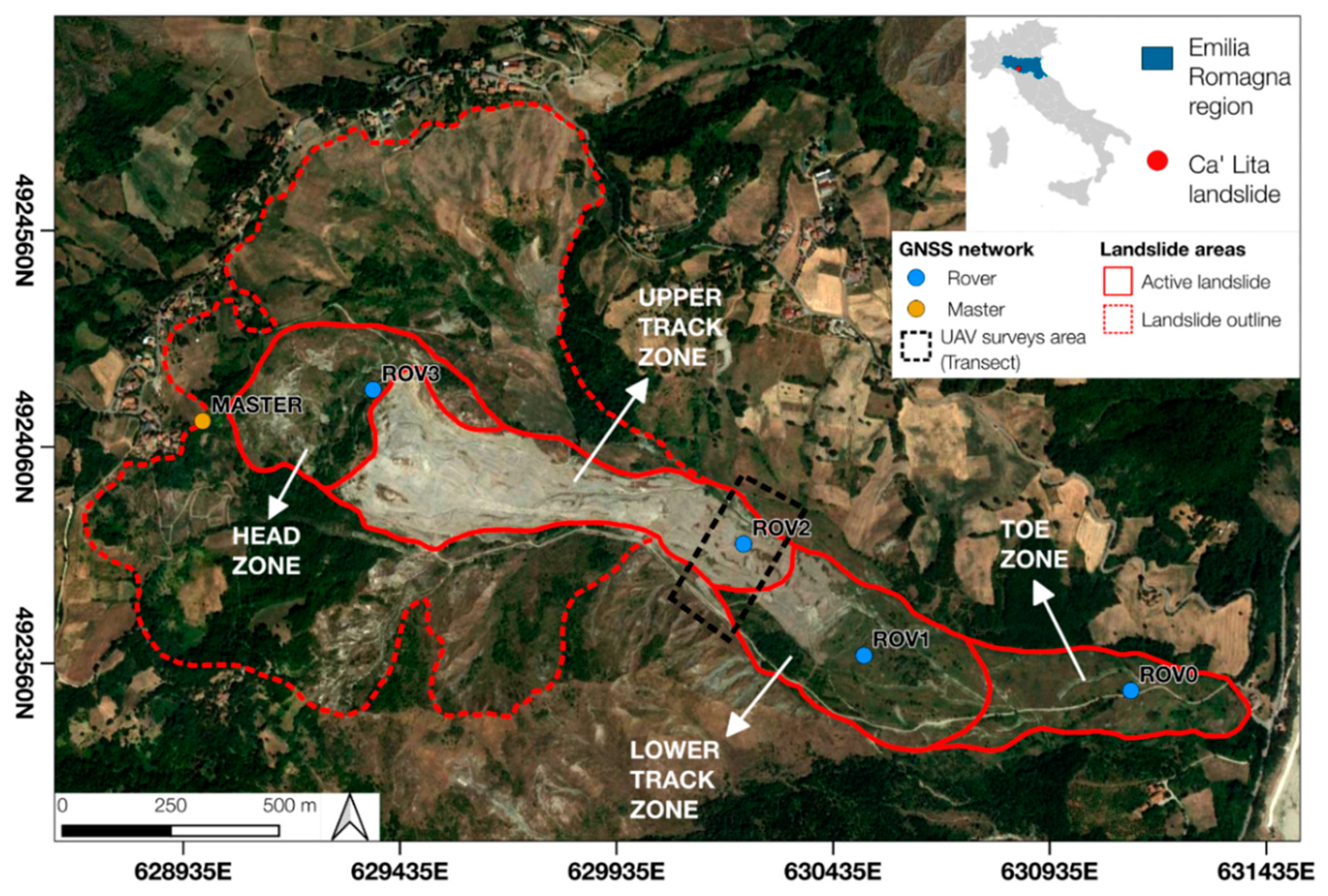
2. Case Study
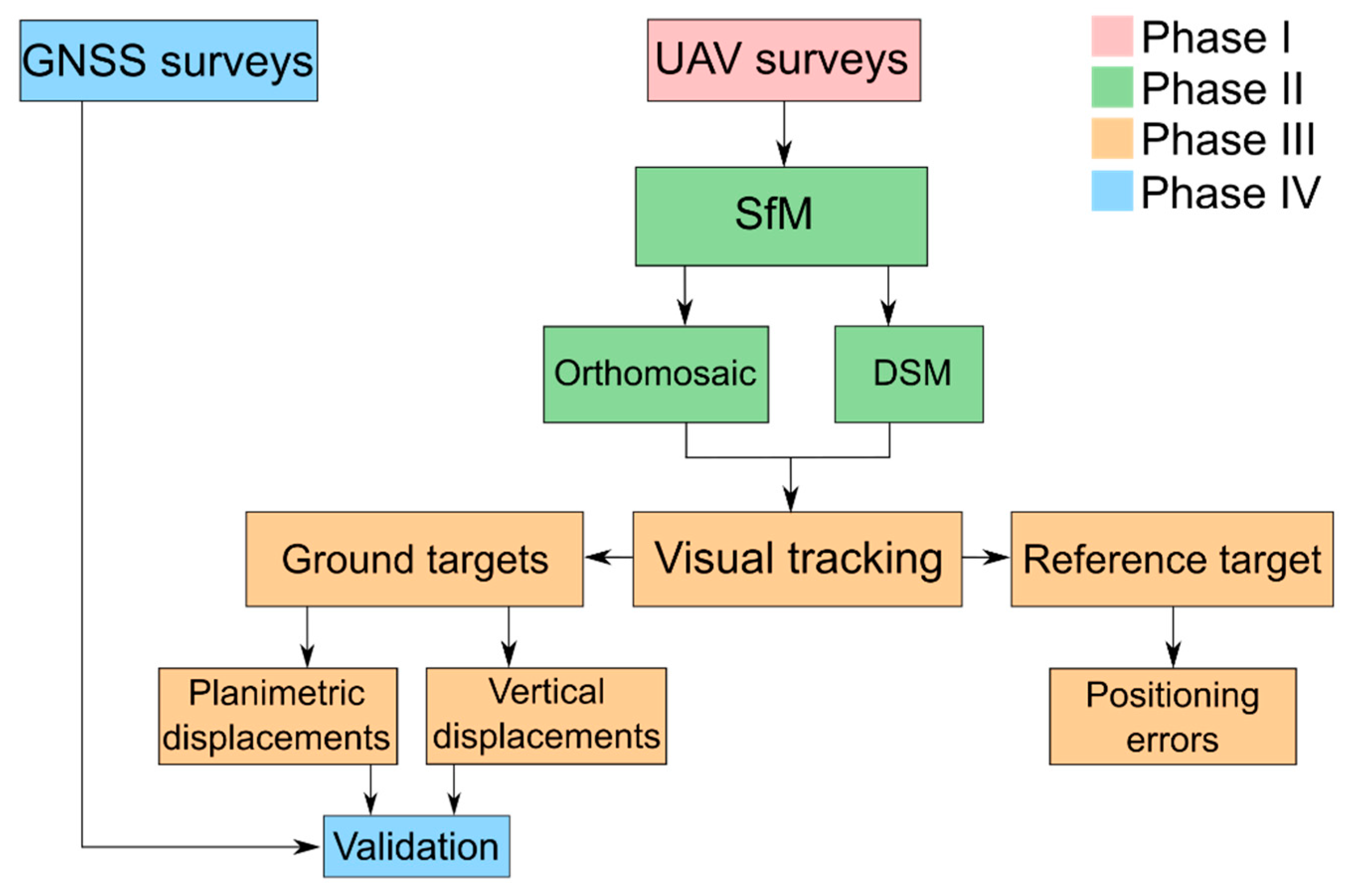
3. Materials and Methods
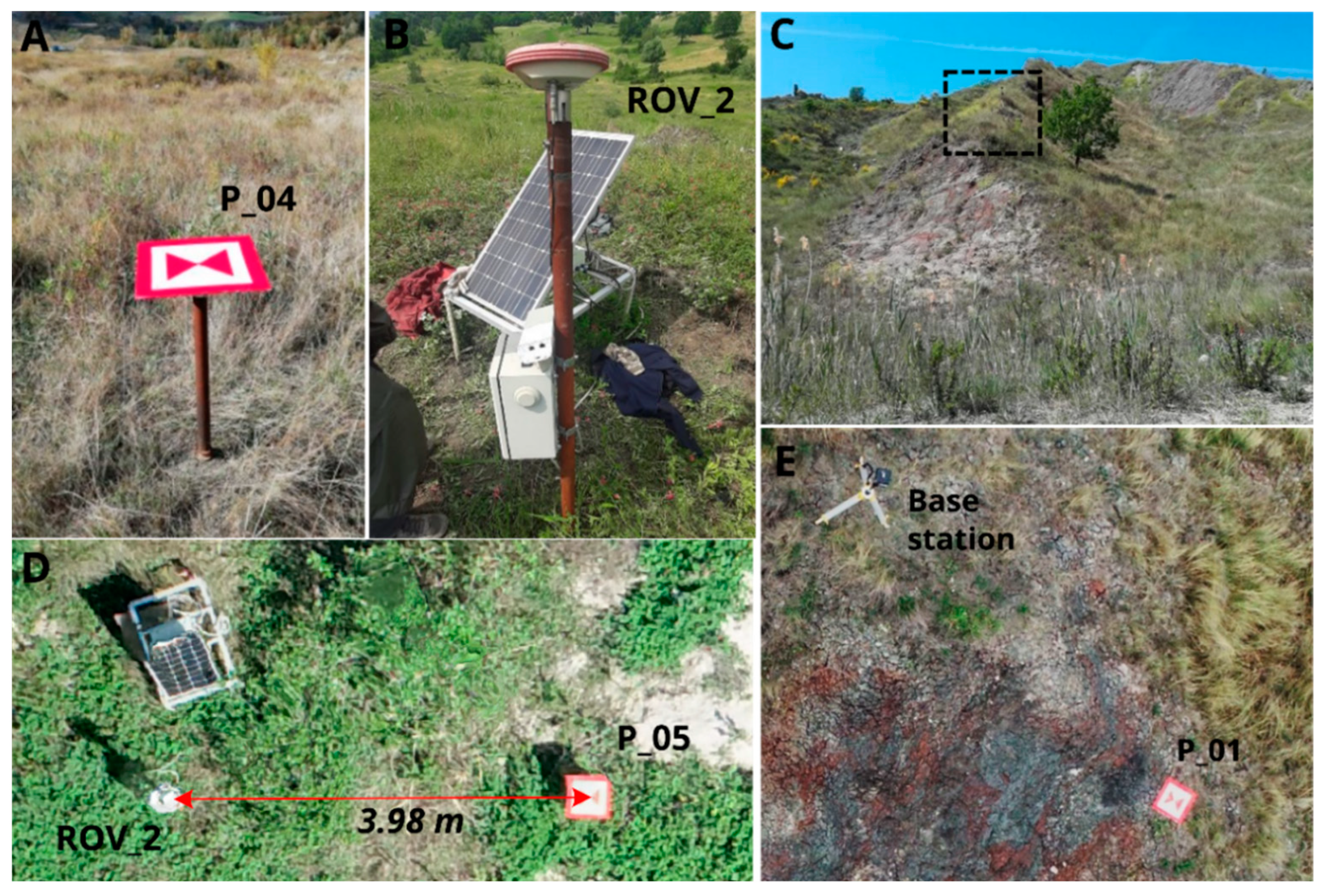
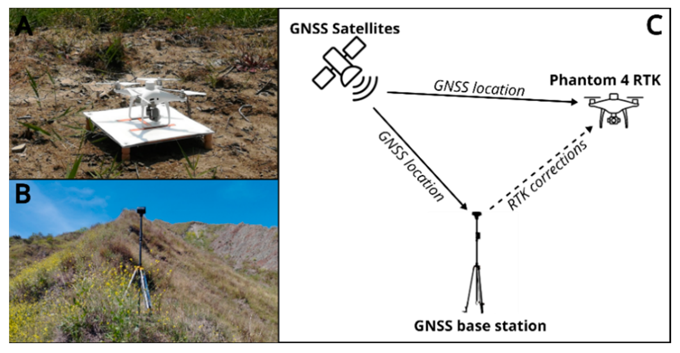
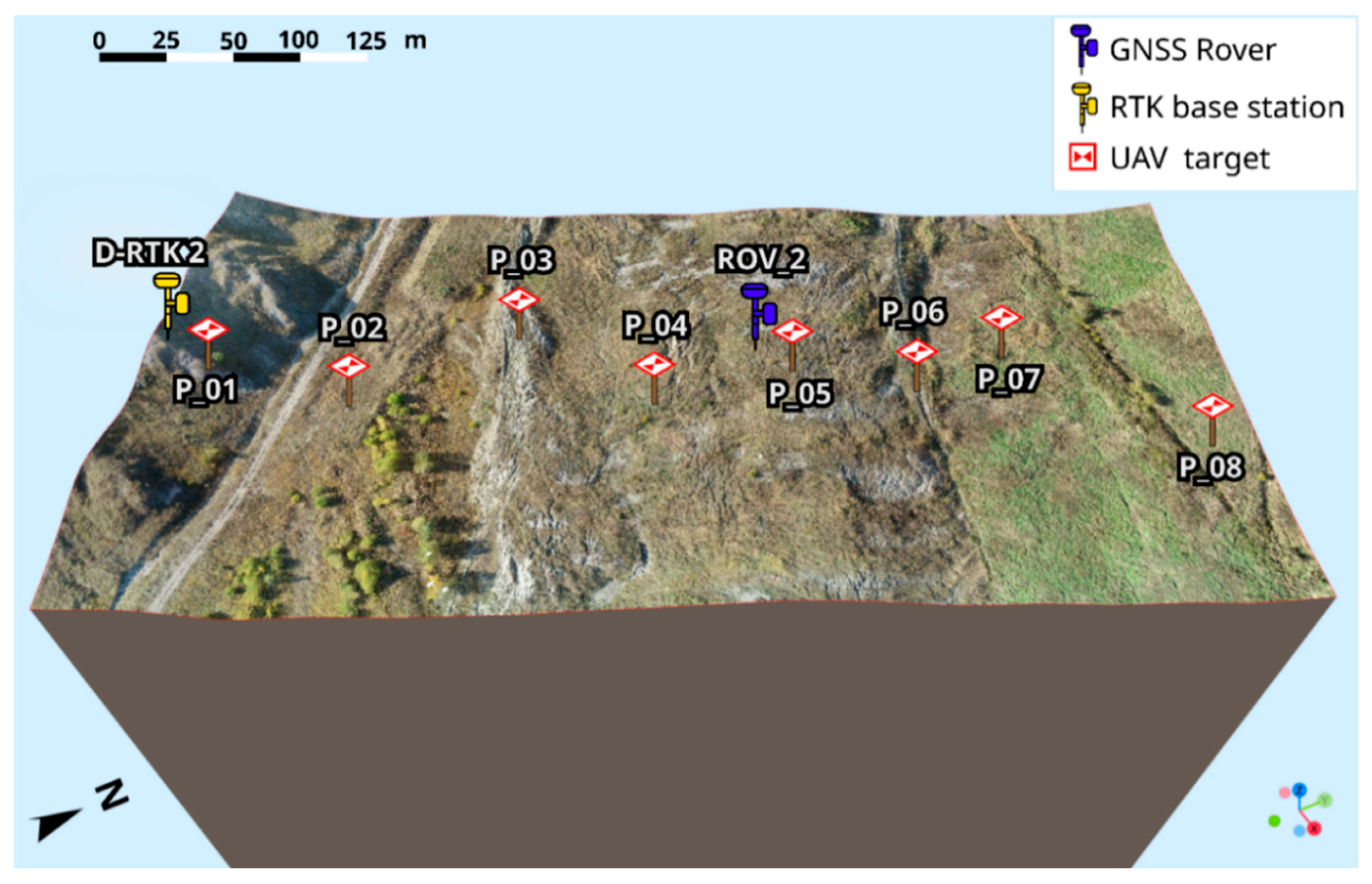
3.1. UAV Monitoring
3.2. Target Visual Tracking
3.3. Continuous GNSS Monitoring
3.4. Methods for Error Estimation and Result Validation
4. Results and Discussion
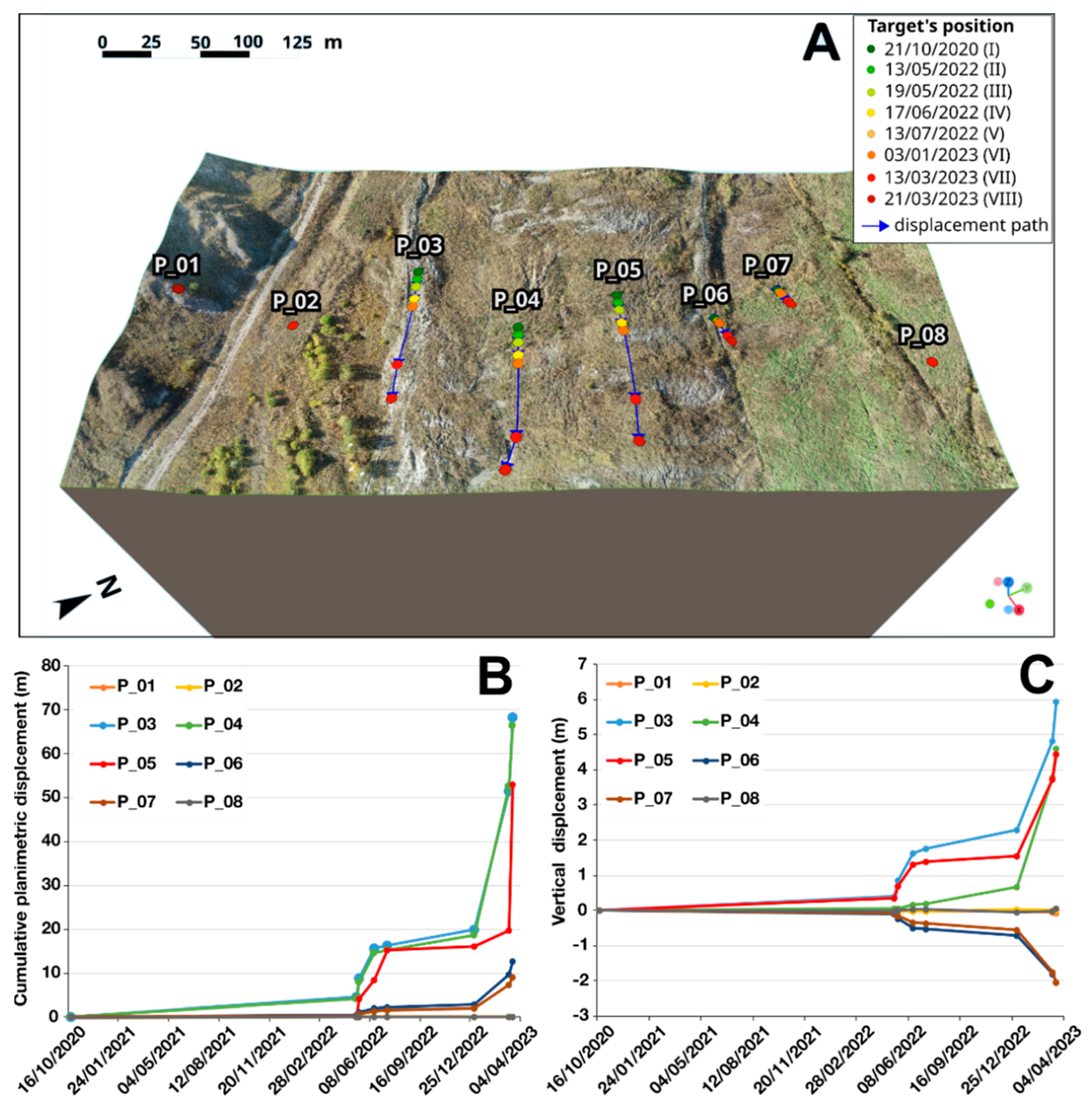
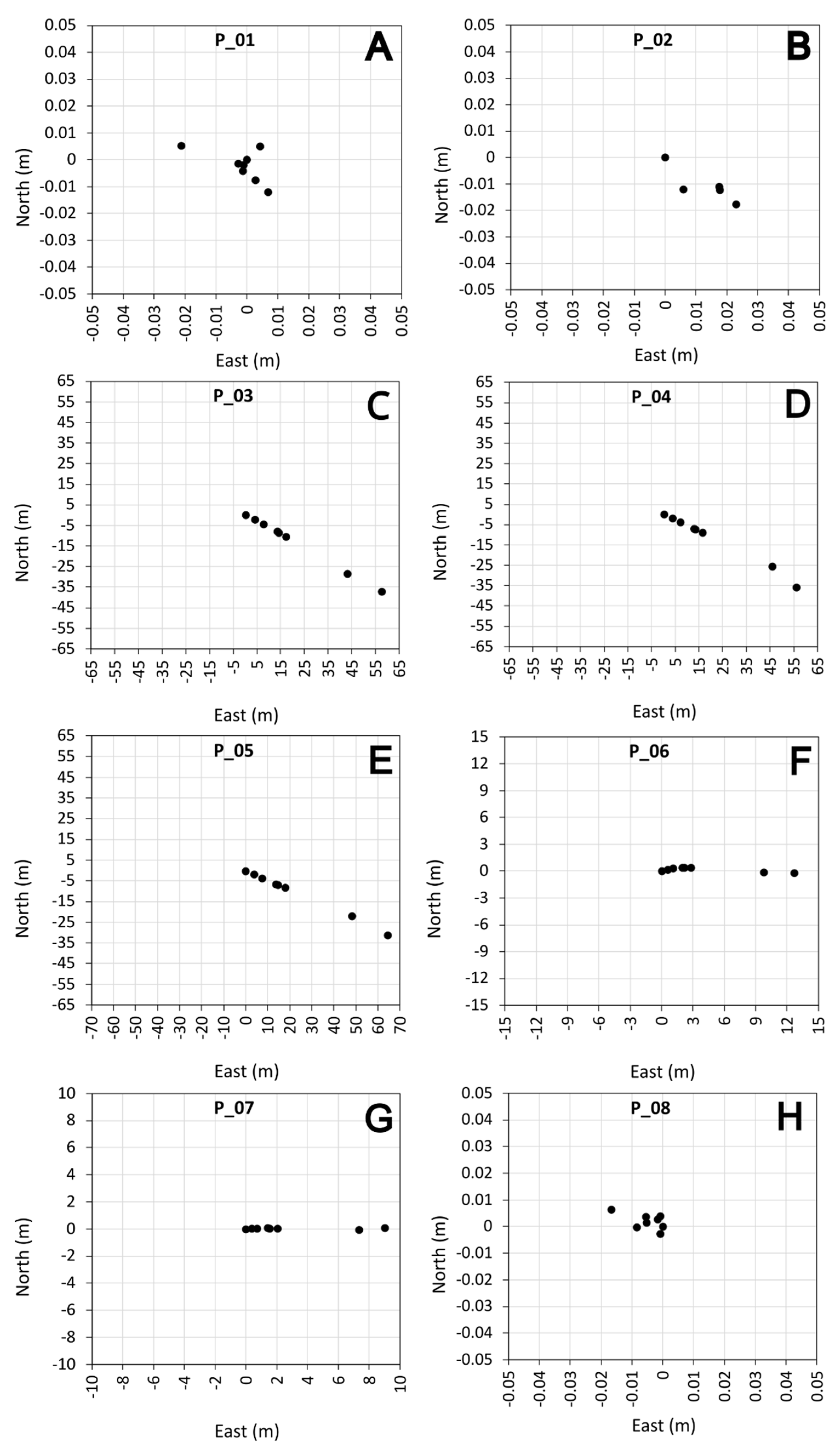
4.1. Ground-Target Displacements
4.2. Detecting Landslides’ Dynamics
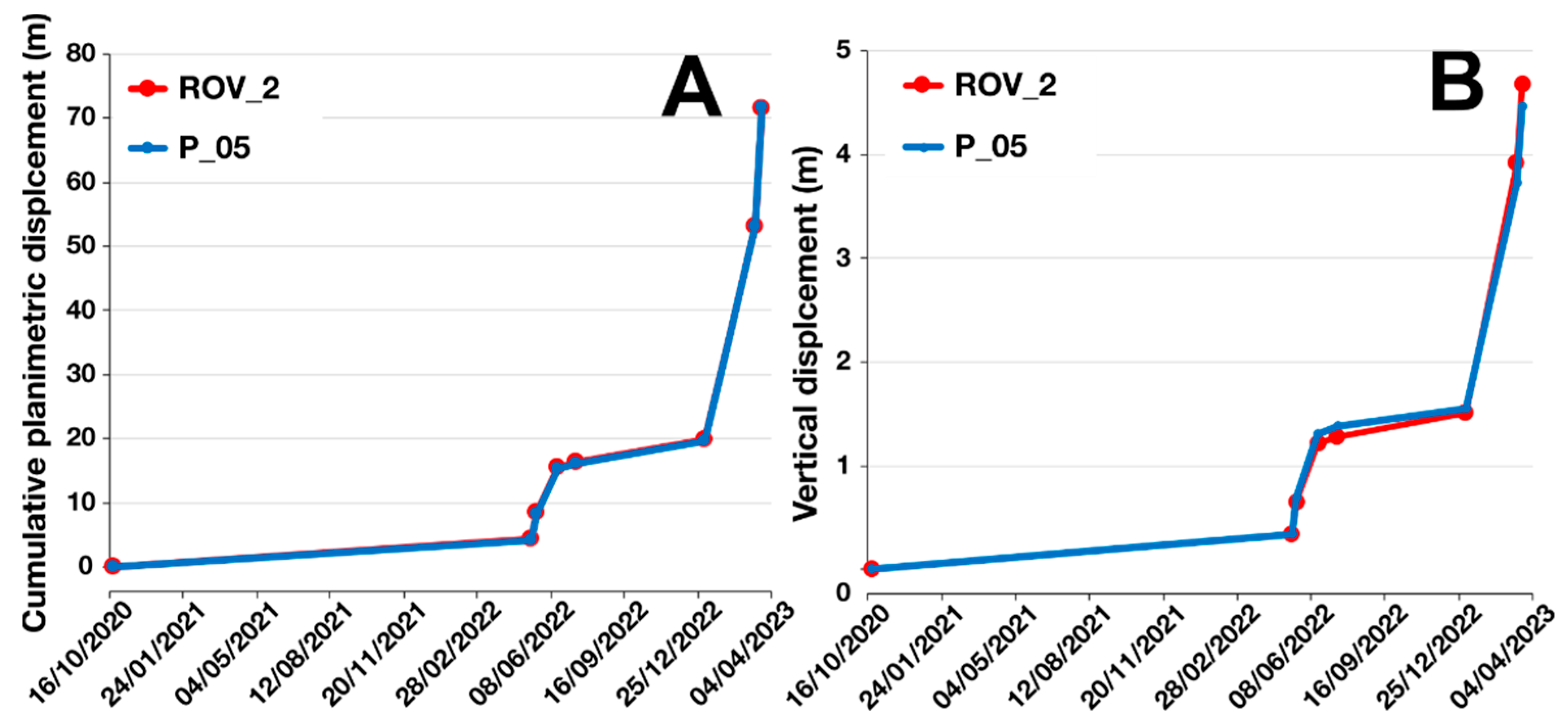
4.3. GNSS Displacements
4.4. Error Estimation and Result Validation
5. Conclusions
Author Contributions
Funding
Data Availability Statement
Conflicts of Interest
Appendix A

| Surveys | P_01 | P_02 | P_03 | ||||||
|---|---|---|---|---|---|---|---|---|---|
| E | N | H | E | N | H | E | N | H | |
| I | 630,130.388 | 4,923,669.228 | 393.775 | 630,167.219 | 4,923,707.446 | 381.878 | 630,167.791 | 4,923,767.687 | 386.021 |
| II | 630,130.386 | 4,923,669.224 | 393.770 | 630,167.236 | 4,923,707.435 | 381.890 | 630,171.830 | 4,923,765.462 | 385.613 |
| III | 630,130.392 | 4,923,669.233 | 393.742 | 630,167.237 | 4,923,707.434 | 381.845 | 630,175.317 | 4,923,763.228 | 385.161 |
| IV | 630,130.366 | 4,923,669.234 | 393.743 | 630,167.225 | 4,923,707.434 | 381.848 | 630,181.154 | 4,923,759.712 | 384.391 |
| V | 630,130.385 | 4,923,669.227 | 393.752 | 630,167.242 | 4,923,707.428 | 381.862 | 630,181.840 | 4,923,759.277 | 384.260 |
| VI | 630,130.387 | 4,923,669.226 | 393.749 | 630,167.272 | 4,923,707.410 | 381.918 | 630,184.824 | 4,923,757.271 | 383.739 |
| VII | 630,130.390 | 4,923,669.221 | 393.717 | 630,167.299 | 4,923,707.405 | 381.890 | 630,210.669 | 4,923,739.122 | 381.191 |
| VIII | 630,130.394 | 4,923,669.216 | 393.699 | 630,167.306 | 4,923,707.406 | 381.880 | 630,225.157 | 4,923,730.578 | 380.086 |
| Surveys | P_04 | P_05 | P_06 | ||||||
| E | N | H | E | N | H | E | N | H | |
| I | 630,221.011 | 4,923,791.641 | 381.824 | 630,228.221 | 4,923,837.489 | 386,412 | 630,258.181 | 4,923,869.607 | 380.921 |
| II | 630,224.604 | 4,923,789.700 | 381.779 | 630,232.029 | 4,923,835.677 | 386.075 | 630,258.745 | 4,923,869.779 | 381.034 |
| III | 630,228.059 | 4,923,787.838 | 381.766 | 630,235.780 | 4,923,833.941 | 385.722 | 630,259.270 | 4,923,869.925 | 381.165 |
| IV | 630,233.779 | 4,923,784.761 | 381.667 | 630,242.156 | 4,923,831.075 | 385.106 | 630,260.150 | 4,923,870.013 | 381.419 |
| V | 630,234.455 | 4,923,784.410 | 381.638 | 630,242.897 | 4,923,830.758 | 385.035 | 630,260.315 | 4,923,870.014 | 381.447 |
| VI | 630,237.429 | 4,923,782.794 | 381.146 | 630,246.122 | 4,923,829.348 | 384.864 | 630,260.968 | 4,923,869.985 | 381.640 |
| VII | 630,266.803 | 4,923,766.072 | 378.026 | 630,276.498 | 4,923,815.549 | 382.684 | 630,267.917 | 4,923,869.486 | 382.723 |
| VIII | 630,276.962 | 4,923,755.886 | 377.206 | 630,292.735 | 4,923,806.421 | 381.95 | 630,270.872 | 4,923,869.392 | 382.960 |
| Surveys | P_07 | P_08 | ROV_2 | ||||||
| E | N | H | E | N | H | E | N | H | |
| I | 630,258.232 | 4,923,905.730 | 380.517 | 630,321.215 | 4,923,936.680 | 381.588 | 630,224.257 | 4,923,838.4970 | 389.4624 |
| II | 630,258.625 | 4,923,905.748 | 380.601 | 630,321.207 | 4,923,936.680 | 381.621 | 630,228.090 | 4,923,836.6310 | 389.1286 |
| III | 630,258.967 | 4,923,905.775 | 380.675 | 630,321.215 | 4,923,936.682 | 381.578 | 630,231.865 | 4,923,834.8610 | 388.8185 |
| IV | 630,259.632 | 4,923,905.803 | 380.859 | 630,321.199 | 4,923,936.673 | 381.565 | 630,238.250 | 4,923,831.9900 | 388.2529 |
| V | 630,259.754 | 4,923,905.781 | 380.883 | 630,321.215 | 4,923,936.675 | 381.556 | 630,238.984 | 4,923,831.6731 | 388.1872 |
| VI | 630,260.289 | 4,923,905.757 | 381.065 | 630,321.210 | 4,923,936.676 | 381.631 | 630,242.205 | 4,923,830.2735 | 387.9538 |
| VII | 630,265.555 | 4,923,905.693 | 382.287 | 630,321.210 | 4,923,936.678 | 381.609 | 630,272.642 | 4,923,816.7628 | 385.5506 |
| VIII | 630,267.240 | 4,923,905.842 | 382.567 | 630,321.214 | 4,923,936.677 | 381.536 | 630,288.691 | 4,923,807.6730 | 384.7922 |
References
- Turner, D.; Lucieer, A.; de Jong, S.M. Time Series Analysis of Landslide Dynamics Using an Unmanned Aerial Vehicle (UAV). Remote Sens. 2015, 7, 1736–1757. [Google Scholar] [CrossRef]
- Mantovani, M.; Bossi, G.; Dykes, A.P.; Pasuto, A.; Soldati, M.; Devoto, S. Coupling Long-Term GNSS Monitoring and Numerical Modelling of Lateral Spreading for Hazard Assessment Purposes. Eng. Geol. 2022, 296, 106466. [Google Scholar] [CrossRef]
- Palis, E.; Lebourg, T.; Tric, E.; Malet, J.P.; Vidal, M. Long-Term Monitoring of a Large Deep-Seated Landslide (La Clapiere, South-East French Alps): Initial Study. Landslides 2017, 14, 155–170. [Google Scholar] [CrossRef]
- Gullà, G.; Calcaterra, S.; Gambino, P.; Borrelli, L.; Muto, F. Long-Term Measurements Using an Integrated Monitoring Network to Identify Homogeneous Landslide Sectors in a Complex Geo-Environmental Context (Lago, Calabria, Italy). Landslides 2018, 15, 1503–1521. [Google Scholar] [CrossRef]
- Malet, J.-P.; Maquaire, O.; Calais, E. The Use of Global Positioning System Techniques for the Continuous Monitoring of Landslides: Application to the Super-Sauze Earthf Low (Alpes-de-Haute-Provence, France). Geomorphology 2002, 43, 33–54. [Google Scholar] [CrossRef]
- Aguzzoli, A.; Arosio, D.; Mulas, M.; Ciccarese, G.; Bayer, B.; Winkler, G.; Ronchetti, F. Multidisciplinary Non-Invasive Investigations to Develop a Hydrogeological Conceptual Model Supporting Slope Kinematics at Fontana Cornia Landslide, Northern Apennines, Italy. Environ. Earth Sci. 2022, 81, 471. [Google Scholar] [CrossRef]
- Hojat, A.; Arosio, D.; Ivanov, V.I.; Longoni, L.; Papini, M.; Scaioni, M.; Tresoldi, G.; Zanzi, L. Geoelectrical Characterization and Monitoring of Slopes on a Rainfall-Triggered Landslide Simulator. J. Appl. Geophys. 2019, 170, 103844. [Google Scholar] [CrossRef]
- Zhang, Z.; Arosio, D.; Hojat, A.; Zanzi, L. Tomographic Experiments for Defining the 3D Velocity Model of an Unstable Rock Slope to Support Microseismic Event Interpretation. Geosciences 2020, 10, 327. [Google Scholar] [CrossRef]
- Mulas, M.; Marnas, M.; Ciccarese, G.; Corsini, A. Sinusoidal Wave Fit Indexing of Irreversible Displacements for Crackmeters Monitoring of Rockfall Areas: Test at Pietra Di Bismantova (Northern Apennines, Italy). Landslides 2020, 17, 231–240. [Google Scholar] [CrossRef]
- Agostini, A.; Tofani, V.; Nolesini, T.; Gigli, G.; Tanteri, L.; Rosi, A.; Cardellini, S.; Casagli, N. A New Appraisal of the Ancona Landslide Based on Geotechnical Investigations and Stability Modelling. Q. J. Eng. Geol. Hydrogeol. 2014, 47, 29–44. [Google Scholar] [CrossRef]
- Azmoon, B.; Biniyaz, A.; Liu, Z. Use of High-Resolution Multi-Temporal DEM Data for Landslide Detection. Geoscience 2022, 12, 378. [Google Scholar] [CrossRef]
- Ghirotti, M.; Donati, D.; Stead, D. Editorial: Developments of Remote Sensing and Numerical Modeling Applications for Landslide Analysis. Front. Earth Sci. 2023, 10, 1129733. [Google Scholar] [CrossRef]
- Dematteis, N.; Wrzesniak, A.; Allasia, P.; Bertolo, D.; Giordan, D. Integration of Robotic Total Station and Digital Image Correlation to Assess the Three-Dimensional Surface Kinematics of a Landslide. Eng. Geol. 2022, 303, 106655. [Google Scholar] [CrossRef]
- Corsini, A.; Bonacini, F.; Mulas, M.; Petitta, M.; Ronchetti, F.; Truffelli, G. Long-Term Continuous Monitoring of a Deep-Seated Compound Rock Slide in the Northern Apennines (Italy). Eng. Geol. Soc. Territ. 2015, 2, 1337–1340. [Google Scholar] [CrossRef]
- Frigerio, S.; Schenato, L.; Bossi, G.; Cavalli, M.; Mantovani, M.; Marcato, G.; Pasuto, A. A Web-Based Platform for Automatic and Continuous Landslide Monitoring: The Rotolon (Eastern Italian Alps) Case Study. Comput. Geosci. 2014, 63, 96–105. [Google Scholar] [CrossRef]
- Baldi, P.; Cenni, N.; Fabris, M.; Zanutta, A. Kinematics of a Landslide Derived from Archival Photogrammetry and GPS Data. Geomorphology 2008, 102, 435–444. [Google Scholar] [CrossRef]
- Mora, O.E.; Gabriela Lenzano, M.; Toth, C.K.; Grejner-Brzezinska, D.A.; Fayne, J.V. Landslide Change Detection Based on Multi-Temporal Airborne LIDAR-Derived DEMs. Geosciences 2018, 8, 23. [Google Scholar] [CrossRef]
- Bossi, G.; Cavalli, M.; Crema, S.; Frigerio, S.; Quan Luna, B.; Mantovani, M.; Marcato, G.; Schenato, L.; Pasuto, A. Multi-Temporal LiDAR-DTMs as a Tool for Modelling a Complex Landslide: A Case Study in the Rotolon Catchment (Eastern Italian Alps). Nat. Hazards Earth Syst. Sci. 2015, 15, 715–722. [Google Scholar] [CrossRef]
- Jaboyedoff, M.; Oppikofer, T.; Abellán, A.; Derron, M.H.; Loye, A.; Metzger, R.; Pedrazzini, A. Use of LIDAR in Landslide Investigations: A Review. Nat. Hazards 2012, 61, 5–28. [Google Scholar] [CrossRef]
- Tondo, M.; Mulas, M.; Ciccarese, G.; Marcato, G.; Bossi, G.; Tonidandel, D.; Mair, V.; Corsini, A. Detecting Recent Dynamics in Large-Scale Landslides via the Digital Image Correlation of Airborne Optic and LiDAR Datasets: Test Sites in South Tyrol (Italy). Remote Sens. 2023, 15, 2971. [Google Scholar] [CrossRef]
- Squarzoni, C.; Delacourt, C.; Allemand, P. Nine Years of Spatial and Temporal Evolution of the La Valette Landslide Observed by SAR Interferometry. Eng. Geol. 2003, 68, 53–66. [Google Scholar] [CrossRef]
- Iasio, C.; Novali, F.; Corsini, A.; Mulas, M.; Branzanti, M.; Benedetti, E.; Giannico, C.; Tamburini, A.; Mair, V. COSMO SkyMed High Frequency—High Resolution Monitoring of an Alpine Slow Landslide, Corvara in Badia, Northern Italy. In Proceedings of the 2012 IEEE International Geoscience and Remote Sensing Symposium, Munich, Germany, 22–27 July 2012; pp. 7577–7580. [Google Scholar] [CrossRef]
- Gaidi, S.; Galve, J.P.; Melki, F.; Ruano, P.; Reyes-Carmona, C.; Marzougui, W.; Devoto, S.; Pérez-Peña, J.V.; Azañón, J.M.; Chouaieb, H.; et al. Analysis of the Geological Controls and Kinematics of the Chgega Landslide (Mateur, Tunisia) Exploiting Photogrammetry and Insar Technologies. Remote Sens. 2021, 13, 4048. [Google Scholar] [CrossRef]
- Mateos, R.M.; Ezquerro, P.; Azañón, J.M.; Gelabert, B.; Herrera, G.; Fernández-Merodo, J.A.; Spizzichino, D.; Sarro, R.; García-Moreno, I.; Béjar-Pizarro, M. Coastal Lateral Spreading in the World Heritage Site of the Tramuntana Range (Majorca, Spain). The Use of PSInSAR Monitoring to Identify Vulnerability. Landslides 2018, 15, 797–809. [Google Scholar] [CrossRef]
- Schlögel, R.; Thiebes, B.; Mulas, M.; Cuozzo, G.; Notarnicola, C.; Schneiderbauer, S.; Crespi, M.; Mazzoni, A.; Mair, V.; Corsini, A. Multi-Temporal x-Band Radar Interferometry Using Corner Reflectors: Application and Validation at the Corvara Landslide (Dolomites, Italy). Remote Sens. 2017, 9, 739. [Google Scholar] [CrossRef]
- Mulas, M.; Bayer, B.; Bertolini, G.; Bonacini, F.; Leuratti, E.; Pizziolo, M.; Simoni, A.; Corsini, A. Impulsive Ground Movements in the Mud Volcanoes Area of “Le Sarse” Di Puianello (Northern Apennines, Modena, Italy): Field Evidence and Multi-Approach Monitoring. Rend. Online Della Soc. Geol. Ital. 2016, 41, 251–254. [Google Scholar] [CrossRef]
- Peyret, M.; Djamour, Y.; Rizza, M.; Ritz, J.-F.; Hurtrez, J.-E.; Goudarzi, M.A.; Nankali, H.; Chéry, J.; Le Dortz, K.; Uri, F. Monitoring of the Large Slow Kahrod Landslide in Alborz Mountain Range (Iran) by GPS and SAR Interferometry. Eng. Geol. 2008, 100, 131–141. [Google Scholar] [CrossRef]
- Bovenga, F.; Pasquariello, G.; Pellicani, R.; Refice, A.; Spilotro, G. Landslide Monitoring for Risk Mitigation by Using Corner Reflector and Satellite SAR Interferometry: The Large Landslide of Carlantino (Italy). Catena 2017, 151, 49–62. [Google Scholar] [CrossRef]
- Mulas, M.; Corsini, A.; Cuozzo, G.; Callegari, M.; Thiebes, B.; Mair, V. Quantitative Monitoring of Surface Movements on Active Landslides by Multi-Temporal, High-Resolution X-Band SAR Amplitude Information: Preliminary Results. In Landslides and Engineered Slopes. Experience, Theory and Practice; CRC Press: Boca Raton, FL, USA, 2016; pp. 1511–1516. [Google Scholar] [CrossRef]
- Qu, T.; Lu, P.; Liu, C.; Wu, H.; Shao, X.; Wan, H.; Li, N.; Li, R. Hybrid-SAR Technique: Joint Analysis Using Phase-Based and Amplitude-Based Methods for the Xishancun Giant Landslide Monitoring. Remote Sens. 2016, 8, 874. [Google Scholar] [CrossRef]
- Wang, M.; Zhou, J.; Chen, J.; Jiang, N.; Zhang, P.; Li, H. Automatic Identification of Rock Discontinuity and Stability Analysis of Tunnel Rock Blocks Using Terrestrial Laser Scanning. J. Rock Mech. Geotech. Eng. 2023, 15, 1810–1825. [Google Scholar] [CrossRef]
- Abellán, A.; Calvet, J.; Vilaplana, J.M.; Blanchard, J. Detection and Spatial Prediction of Rockfalls by Means of Terrestrial Laser Scanner Monitoring. Geomorphology 2010, 119, 162–171. [Google Scholar] [CrossRef]
- Corsini, A.; Castagnetti, C.; Bertacchini, E.; Rivola, R.; Ronchetti, F.; Capra, A. Integrating Airborne and Multi-temporal Long-range Terrestrial Laser Scanning with Total Station Measurements for Mapping and Monitoring a Compound Slow Moving Rock Slide. Earth Surf. Process Landf. 2013, 38, 1330–1338. [Google Scholar] [CrossRef]
- Giordan, D.; Hayakawa, Y.; Nex, F.; Remondino, F.; Tarolli, P. Review Article: The Use of Remotely Piloted Aircraft Systems (RPASs) for Natural Hazards Monitoring and Management. Nat. Hazards Earth Syst. Sci. 2018, 18, 1079–1096. [Google Scholar] [CrossRef]
- Thiebes, B.; Tomellari, E.; Mejia-Aguilar, M.; Rabanser, M.; Schlögel, R.; Mulas, M.; Corsini, A. Assessment of the 2006 to 2015 Corvara Landslide Evolution a UAV-Derived DSM and Orthophoto. In Landslides and Engineered Slopes. Experience, Theory and Practice; CRC Press: Boca Raton, FL, USA, 2018; pp. 1897–1902. [Google Scholar] [CrossRef]
- Sestras, P.; Bilașco, Ș.; Roșca, S.; Dudic, B.; Hysa, A.; Spalević, V. Geodetic and UAV Monitoring in the Sustainable Management of Shallow Landslides and Erosion of a Susceptible Urban Environment. Remote Sens. 2021, 13, 385. [Google Scholar] [CrossRef]
- Mugnai, F.; Tucci, G. A Comparative Analysis of Unmanned Aircraft Systems in Low Altitude Photogrammetric Surveys. Remote Sens. 2022, 14, 726. [Google Scholar] [CrossRef]
- Westoby, M.J.; Brasington, J.; Glasser, N.F.; Hambrey, M.J.; Reynolds, J.M. “Structure-from-Motion” Photogrammetry: A Low-Cost, Effective Tool for Geoscience Applications. Geomorphology 2012, 179, 300–314. [Google Scholar] [CrossRef]
- Peppa, M.V.; Mills, J.P.; Moore, P.; Miller, P.E.; Chambers, J.E. Automated Co-registration and Calibration in SfM Photogrammetry for Landslide Change Detection. Earth Surf. Process Landf. 2019, 44, 287–303. [Google Scholar] [CrossRef]
- Godone, D.; Allasia, P.; Borrelli, L.; Gullà, G. UAV and Structure from Motion Approach to Monitor the Maierato Landslide Evolution. Remote Sens. 2020, 12, 1039. [Google Scholar] [CrossRef]
- Eker, R.; Alkan, E.; Aydin, A. A Comparative Analysis of UAV-RTK and UAV-PPK Methods in Mapping Different Surface Types. Eur. J. For. Eng. 2021, 7, 12–25. [Google Scholar] [CrossRef]
- Tavani, S.; Granado, P.; Riccardi, U.; Seers, T.; Corradetti, A. Terrestrial SfM-MVS Photogrammetry from Smartphone Sensors. Geomorphology 2020, 367, 107318. [Google Scholar] [CrossRef]
- Mazza, D.; Romeo, S.; Cosentino, A.; Mazzanti, P.; Guadagno, F.M.; Revellino, P. The Contribution of Digital Image Correlation for the Knowledge, Control and Emergency Monitoring of Earth Flows. Geosciences 2023, 13, 364. [Google Scholar] [CrossRef]
- Casagli, N.; Frodella, W.; Morelli, S.; Tofani, V.; Ciampalini, A.; Intrieri, E.; Raspini, F.; Rossi, G.; Tanteri, L.; Lu, P. Spaceborne, UAV and Ground-Based Remote Sensing Techniques for Landslide Mapping, Monitoring and Early Warning. Geoenviron. Disasters 2017, 4, 9. [Google Scholar] [CrossRef]
- Tang, C.; Wang, Y.; Zhang, L.; Zhang, Y. GNSS/Inertial Navigation/Wireless Station Fusion UAV 3-D Positioning Algorithm With Urban Canyon Environment. IEEE Sens. J. 2022, 22, 18771–18779. [Google Scholar] [CrossRef]
- Martínez-Carricondo, P.; Agüera-Vega, F.; Carvajal-Ramírez, F. Accuracy Assessment of RTK/PPK UAV-Photogrammetry Projects Using Differential Corrections from Multiple GNSS Fixed Base Stations. Geocarto Int. 2023, 38, 2197507. [Google Scholar] [CrossRef]
- Taddia, Y.; Stecchi, F.; Pellegrinelli, A. Using DJI Phantom 4 RTK Drone for Topographic Mapping of Coastal Areas. Int. Arch. Photogramm. Remote Sens. Spat. Inf. Sci. 2019, XLII-2/W13, 625–630. [Google Scholar] [CrossRef]
- Kalacska, M.; Lucanus, O.; Arroyo-Mora, J.P.; Laliberté, É.; Elmer, K.; Leblanc, G.; Groves, A. Accuracy of 3d Landscape Reconstruction without Ground Control Points Using Different Uas Platforms. Drones 2020, 4, 13. [Google Scholar] [CrossRef]
- Stott, E.; Williams, R.D.; Hoey, T.B. Ground Control Point Distribution for Accurate Kilometre-Scale Topographic Mapping Using an Rtk-Gnss Unmanned Aerial Vehicle and Sfm Photogrammetry. Drones 2020, 4, 55. [Google Scholar] [CrossRef]
- Peppa, M.V.; Hall, J.; Goodyear, J.; Mills, J.P. Photogrammetric Assessment and Comparison of Dji Phantom 4 pro and Phantom 4 Rtk Small Unmanned Aircraft Systems. Int. Arch. Photogramm. Remote Sens. Spat. Inf. Sci. ISPRS Arch. 2019, 42, 503–509. [Google Scholar] [CrossRef]
- Notti, D.; Giordan, D.; Cina, A.; Manzino, A.; Maschio, P.; Bendea, I.H. Debris Flow and Rockslide Analysis with Advanced Photogrammetry Techniques Based on High-Resolution RPAS Data. Ponte Formazza Case Study (NW Alps). Remote Sens. 2021, 13, 1797. [Google Scholar] [CrossRef]
- Cruden, D.M.; Varnes, D.J. Landslide Types and Processes. In Landslides: Investigation and Mitigation; Volume Special Report 247; National Academy Press: Washington, DC, USA, 1996; pp. 36–75. ISBN 030906208X. [Google Scholar]
- Corsini, A.; Borgatti, L.; Caputo, G.; De Simone, N.; Sartini, G.; Truffelli, G. Investigation and Monitoring in Support of the Structural Mitigation of Large Slow Moving Landslides: An Example from Ca’ Lita (Northern Apennines, Reggio Emilia, Italy). Nat. Hazards Earth Syst. Sci. 2006, 6, 55–61. [Google Scholar] [CrossRef]
- Borgatti, L.; Corsini, A.; Barbieri, M.; Sartini, G.; Truffelli, G.; Caputo, G.; Puglisi, C. Large Reactivated Landslides in Weak Rock Masses: A Case Study from the Northern Apennines (Italy). Landslides 2006, 3, 115–124. [Google Scholar] [CrossRef]
- Mulas, M.; Ciccarese, G.; Truffelli, G.; Corsini, A. Integration of Digital Image Correlation of Sentinel-2 Data and Continuous GNSS for Long-Term Slope Movements Monitoring in Moderately Rapid Landslides. Remote Sens. 2020, 12, 2605. [Google Scholar] [CrossRef]
- Antolini, G.; Auteri, L.; Pavan, V.; Tomei, F.; Tomozeiu, R.; Marletto, V. A Daily High-Resolution Gridded Climatic Data Set for Emilia-Romagna, Italy, during 1961–2010. Int. J. Climatol. 2016, 36, 1970–1986. [Google Scholar] [CrossRef]
- Arpae Agenzia Prevenzione Ambiente Energia Emilia-Romagna. Tabelle Climatologiche. Available online: https://www.arpae.it/it/temi-ambientali/clima/dati-e-indicatori/tabelle-climatiche (accessed on 4 March 2024).
- Köppen, W. Das Geographische System Der Klimate. In Handbuch der Klimatologie; Gebrüder Borntraeger: Berlin, Germany, 1936. [Google Scholar]
- Borgatti, L.; Corsini, A.; Marcato, G.; Ronchetti, F.; Zabuski, L. Appraise the Structural Mitigation of Landslide Risk via Numerical Modelling: A Case Study from the Northern Apennines (Italy). Georisk 2008, 2, 141–160. [Google Scholar] [CrossRef]
- Cervi, F.; Ronchetti, F.; Martinelli, G.; Bogaard, T.A.; Corsini, A. Origin and Assessment of Deep Groundwater Inflow in the Ca’ Lita Landslide Using Hydrochemistry and in Situ Monitoring. Hydrol. Earth Syst. Sci. 2012, 16, 4205–4221. [Google Scholar] [CrossRef]
- Ronchetti, F.; Borgatti, L.; Cervi, F.; Corsini, A. Hydro-Mechanical Features of Landslide Reactivation in Weak Clayey Rock Masses. Bull. Eng. Geol. Environ. 2010, 69, 267–274. [Google Scholar] [CrossRef]
- Mulas, M.; Ciccarese, G.; Truffelli, G.; Corsini, A. Displacements of an Active Moderately Rapid Landslide—A Dataset Retrieved by Continuous GNSS Arrays. Data 2020, 5, 71. [Google Scholar] [CrossRef]
- Corsini, A.; Bonacini, F.; Mulas, M.; Ronchetti, F.; Monni, A.; Pignone, S.; Primerano, S.; Bertolini, G.; Caputo, G.; Truffelli, G.; et al. A Portable Continuous GPS Array Used as Rapid Deployment Monitoring System during Landslide Emergencies in Emilia Romagna. Rend. Online Della Soc. Geol. Ital. 2015, 35, 89–91. [Google Scholar] [CrossRef]
- Brooke-Holland, L. Unmanned Aerial Vehicles (Drones): An Introduction; House of Commons Library: London, UK, 2012. [Google Scholar]
- Turner, A.K.; Schuster, R.L. Landslides: Investigation and Mitigation; Volume Special Report 247; National Academy Press: Washington, DC, USA, 1996; ISBN 030906208X. [Google Scholar]
- Mugnai, F.; Angelini, R.; Cortesi, I.; Masiero, A. Integrating UAS Photogrammetry and Digital Image Correla-Tion for High-Resolution Monitoring of Large Landslides. Preprints 2022. [Google Scholar] [CrossRef]
- Everett, M.E.; DeSmet, T.S.; Warden, R.R.; Ruiz-Guzman, H.A.; Gavette, P.; Hagin, J. The Fortress beneath: Ground Penetrating Radar Imaging of the Citadel at Alcatraz: 1. A Guide for Interpretation. Heritage 2021, 4, 1328–1347. [Google Scholar] [CrossRef]


| UAV Surveys | |
|---|---|
| Survey | Date (YYYY/MM/DD) |
| I | 2020/10/21 |
| II | 2022/05/13 |
| III | 2022/05/19 |
| IV | 2022/06/17 |
| V | 2022/07/13 |
| VI | 2023/01/03 |
| VII | 2023/03/13 |
| VIII | 2023/03/21 |
| UAV Flight Parameters | |
|---|---|
| Altitude above ground | 37 m |
| Speed (m/s) | 2.9 m/s |
| Ground Sampling Distance (GSD) | 1.01 cm/px |
| Image forward overlap | 70% |
| Image side overlap | 80% |
| Gimble angle | −90° |
| RTK status | Fixed |
| Flight time | 17 min 9 s |
| Number of photos | 415 |
| UAV weight | 1.391 kg |
| UAV size | 350 mm |
| Surveys | P_01 | P_02 | P_03 | P_04 | P_05 | P_06 | P_07 | P_08 | ||||||||
|---|---|---|---|---|---|---|---|---|---|---|---|---|---|---|---|---|
| Cum. Displ. | ΔH | Cum. Displ. | ΔH | Cum. Displ. | ΔH | Cum. Displ. | ΔH | Cum. Displ. | ΔH | Cum. Displ. | ΔH | Cum. Displ. | ΔH | Cum. Displ. | ΔH | |
| I | 0.00 | 0.00 | 0.00 | 0.00 | 0.00 | 0.00 | 0.00 | 0.00 | 0.00 | 0.00 | 0.00 | 0.00 | 0.00 | 0.00 | 0.00 | 0.00 |
| II | 0.004 | 0.00 | 0.02 | 0.01 | 4.61 | 0.41 | 4.08 | 0.05 | 4.22 | 0.34 | 0.00 | −0.11 | 0.39 | −0.08 | 0.01 | −0.03 |
| III | 0.007 | −0.03 | 0.02 | −0.03 | 8.75 | 0.86 | 8.01 | 0.06 | 8.35 | 0.69 | 0.59 | −0.24 | 0.74 | −0.16 | 0.00 | 0.01 |
| IV | 0.022 | −0.03 | 0.01 | −0.03 | 15.56 | 1.63 | 14.50 | 0.16 | 15.34 | 1.31 | 1.13 | −0.50 | 1.40 | −0.34 | 0.02 | 0.02 |
| V | 0.003 | −0.02 | 0.03 | −0.02 | 16.37 | 1.76 | 15.27 | 0.19 | 16.15 | 1.38 | 2.01 | −0.53 | 1.52 | −0.37 | 0.00 | 0.03 |
| VI | 0.002 | −0.03 | 0.06 | 0.04 | 19.97 | 2.28 | 18.65 | 0.68 | 19.67 | 1.55 | 2.17 | −0.72 | 2.06 | −0.55 | 0.01 | −0.04 |
| VII | 0.008 | −0.06 | 0.09 | 0.01 | 51.52 | 4.83 | 52.45 | 3.80 | 53.03 | 3.73 | 2.81 | −1.80 | 7.32 | −1.77 | 0.01 | −0.02 |
| VIII | 0.014 | −0.08 | 0.10 | 0.00 | 68.32 | 5.94 | 66.40 | 4.62 | 71.61 | 4.46 | 9.74 | −2.04 | 9.01 | −2.05 | 0.00 | 0.05 |
| Surveys | P_05 | ROV_2 | |Δ| (P_05 − ROV_2) | |||
|---|---|---|---|---|---|---|
| Cum. Displ. | ΔH | Cum. Displ. | ΔH | Cum. Displ. | ΔH | |
| I | 0.00 | 0.00 | 0.00 | 0.00 | 0.00 | 0.00 |
| II | 4.22 | 0.34 | 4.26 | 0.33 | 0.046 | 0.003 |
| III | 8.35 | 0.69 | 8.43 | 0.64 | 0.082 | 0.046 |
| IV | 15.34 | 1.31 | 15.43 | 1.21 | 0.093 | 0.097 |
| V | 16.15 | 1.38 | 16.23 | 1.28 | 0.086 | 0.102 |
| VI | 19.67 | 1.55 | 19.74 | 1.51 | 0.077 | 0.039 |
| VII | 53.03 | 3.73 | 53.04 | 3.91 | 0.013 | 0.184 |
| VIII | 71.61 | 4.46 | 71.43 | 4.67 | 0.178 | 0.208 |
Disclaimer/Publisher’s Note: The statements, opinions and data contained in all publications are solely those of the individual author(s) and contributor(s) and not of MDPI and/or the editor(s). MDPI and/or the editor(s) disclaim responsibility for any injury to people or property resulting from any ideas, methods, instructions or products referred to in the content. |
© 2024 by the authors. Licensee MDPI, Basel, Switzerland. This article is an open access article distributed under the terms and conditions of the Creative Commons Attribution (CC BY) license (https://creativecommons.org/licenses/by/4.0/).
Share and Cite
Ciccarese, G.; Tondo, M.; Mulas, M.; Bertolini, G.; Corsini, A. Rapid Assessment of Landslide Dynamics by UAV-RTK Repeated Surveys Using Ground Targets: The Ca’ Lita Landslide (Northern Apennines, Italy). Remote Sens. 2024, 16, 1032. https://doi.org/10.3390/rs16061032
Ciccarese G, Tondo M, Mulas M, Bertolini G, Corsini A. Rapid Assessment of Landslide Dynamics by UAV-RTK Repeated Surveys Using Ground Targets: The Ca’ Lita Landslide (Northern Apennines, Italy). Remote Sensing. 2024; 16(6):1032. https://doi.org/10.3390/rs16061032
Chicago/Turabian StyleCiccarese, Giuseppe, Melissa Tondo, Marco Mulas, Giovanni Bertolini, and Alessandro Corsini. 2024. "Rapid Assessment of Landslide Dynamics by UAV-RTK Repeated Surveys Using Ground Targets: The Ca’ Lita Landslide (Northern Apennines, Italy)" Remote Sensing 16, no. 6: 1032. https://doi.org/10.3390/rs16061032
APA StyleCiccarese, G., Tondo, M., Mulas, M., Bertolini, G., & Corsini, A. (2024). Rapid Assessment of Landslide Dynamics by UAV-RTK Repeated Surveys Using Ground Targets: The Ca’ Lita Landslide (Northern Apennines, Italy). Remote Sensing, 16(6), 1032. https://doi.org/10.3390/rs16061032