Abstract
In recent years, hyperspectral (HS) sharpening technology has received high attention and HS sharpened images have been widely applied. However, the quality assessment of HS sharpened images has not been well addressed and is still limited to the use of full-reference quality evaluation. In this paper, a novel no-reference quality assessment method based on Benford’s law for HS sharpened images is proposed. Without a reference image, the proposed method detects fusion distortion by performing first digit distribution on three quality perception features in HS sharpened images, using the standard Benford’s law as a benchmark. The experiment evaluates 10 HS fusion methods on three HS datasets and selects four full-reference metrics and four no-reference metrics to compare with the proposed method. The experimental results demonstrate the superior performance of the proposed method.
1. Introduction
With the rapid development of imaging sensor technology in recent years, more and more airborne and satellite hyperspectral sensors have been able to capture hyperspectral (HS) images. Due to the rich spectral information, HS images have a wide range of applications in remote sensing, such as geological monitoring [1,2,3], object tracking [4], atmospheric monitoring [5,6,7], etc. Because of the trade-off issue in HS images acquisition, where high spectral resolution comes at the cost of low spatial resolution, the practical application of HS data has been greatly limited. In the past decade, many HS sharpening methods have emerged, which produce fused HS images with high spatial resolution (also known as HS sharpened images). In practice, high-quality fused HS images are very desirable in some specific tasks, such as anomaly detection [8], image classification [9], change detection [10], etc. The quality assessment of HS sharpened images is crucial for evaluating the quality of the fusion products from different HS sharpening methods, providing useful feedback to fusion design and valuable guidance for downstream processing tasks.
Nowadays, there are well-known satellites and airborne platforms capturing and providing HS images. The Hyperion sensor equipped on NASA’s Earth Observing-1 satellite (EO-1) can simultaneously capture HS or multispectral (MS) images with a spatial resolution of 30 m and panchromatic (PAN) images with a spatial resolution of 10 m, covering the spectral range of 400–2500 nm [11]. Another famous airborne sensor is the Next-Generation Airborne Visible Infrared Imaging Spectrometer (AVIRIS-NG), which collects HS images from 2012 to the present and supports major activities in North America, India, and Europe [12]. AVIRIS-NG covers a spectral range of 380–2510 nm and has a spatial resolution of 0.3–20 m. The Hyperspectral Imager Suite (HISUI) recently developed by Japan has been recording HS and MS data since 2020, with a spatial resolution of 30 m for HS images and 5 m for MS ones [13]. The Prisma satellite is managed and operated by the Italian Space Agency and was launched in 2019. It collects HS images with a spatial resolution of 30 m and MS images with a spatial resolution of 5 m, covering a spectral range of 400–2500 nm [14]. In addition, the new Environmental Mapping and Analysis Program (EnMAP) HS satellite of Germany was launched in 2022, which can provide 224 bands and has a spectral range of 420–2450 nm, and a spatial resolution of 30 m.
The emergence of new HS sensors and the availability of HS images have stimulated the further development of HS image enhancement technology including HS super resolution and HS sharpening. HS super resolution processes a single input HS image without relying on any auxiliary image/information, while HS sharpening is the fusion of HS images with MS/PAN images to obtain the high spatial resolution HS images. The existing HS sharpening methods can be roughly divided into four categories: classical pansharpening-based methods, matrix factorization (MF)-based methods, tensor representation (TR)-based methods, and deep convolution neural network (CNN)-based methods. Pansharpening (also known as multispectral sharpening) is a traditional fusion technique that utilizes PAN images to improve the spatial resolution of MS images. For the fusion of HS and MS images by using band selection or band synthesis strategy to assign each MS band to several corresponding HS bands, HS sharpening can be seen as an extension of multiple pansharpening [15]. In this way, pansharpening methods can be applied to fuse HS images. Two representative pansharpening methods are component substitution (CS)-based methods and multi-resolution analysis (MRA)-based methods. The former includes intensity–hue–saturation [16], principal component analysis (PCA) [17], Gram-Schmidt adaptive (GSA) [18], etc., while the latter includes the generalized Laplacian pyramid (GLP) [19], smoothing filtered-based intensity modulation (SFIM) [20], etc. MF-based methods is used to estimate the spectral basis and coefficients and regard HS sharpening as an optimization problem. The typical MF-based fusion methods include sparse MF [21], fast fusion based on Sylvester equation [22], non-negative structured sparse representation [23], maximum a posteriori estimation with a stochastic mixing model (MAP-SMM) [24], HS super-resolution (HySure) [25], and coupled non-negative matrix factorization [26]. TR-based methods treat HS and MS data as tensors and decompose them in different ways. Tucker decomposition and Canonical polyadic (CP) decomposition are widely used. The representative TR-based fusion methods include coupled sparse tensor factorization [27], nonlocal coupled tensor CP [28], low tensor multi-rank regularization (LTMR) [29], low tensor-train rank representation [30], unidirectional total variation with tucker decomposition (UTV) [31], tensor subspace representation-based regularization model (IR-TenSR) [32]. The deep CNN-based methods often train a network between ground-truth images (i.e., original HS images) and input images (i.e., low spatial resolution HS and high spatial resolution MS images). In recent years, many deep CNN-based methods have been proposed. The representative deep CNN-based methods include CNN-based fusion (CNN-Fus) [33], two-stream fusion network [34], HS image super-resolution network [35], spatial-spectral residual network [36] and so on. Although there are many different HS sharpening methods, how to accurately evaluate the quality of the HS sharpened images has not been well resolved in the fusion field. Due to the lack of ideal high spatial resolution HS images that can be referenced, no-reference quality assessment of HS sharpened images is still a challenging issue.
In general, quality assessment of fused remote sensing images consists of subjective evaluation and objective evaluation. Subjective evaluation, also known as qualitative evaluation, is the subjective visual evaluation of the fusion result by human observers, and the implementation of the evaluation often requires a lot of manpower and material resources. Objective evaluation, namely quantitative evaluation, is the use of various algorithms or metrics to calculate specific numerical values representing image quality. Figure 1 shows the process of HS sharpening with its objective quality assessment. At present, objective measurement can be classified into full-reference (FR) evaluation and no-reference (NR) evaluation. FR evaluation is more popular, since it is convenient and reliable [37]. FR evaluation needs the reference image as the ground truth and uses it to measure the distorted image. However, the reality is that high spatial resolution (HR) HS images, i.e., the references, are extremely difficult to obtain or do not exist at all. Therefore, FR evaluation of HS sharpened images is usually conducted at a degraded scale. The specific procedure is to degrade both the original HS image and the original HR-MS image to respectively obtain the low spatial resolution (LR) HS image and the degraded LR-MS image. Thus, the original HS image is used as the reference. Then the LR-HS and the LR-MS images are fused together to obtain the fused images (i.e., the HS sharpened images). Finally, the FR quality assessment employs the reference image to measure the distortions of the HS sharpened images. Commonly used FR metrics include peak signal-to-noise ratio (PSNR) [38], spectral angle mapper (SAM) [39], erreur relative globale adimensionnelle de synthèse (ERGAS) [40], structural similarity (SSIM) [41], Q2n [42], etc. Due to the inability of FR assessment to directly provide evaluation results for full-resolution fused images, some scholars shifted the research towards NR evaluation. In recent years, many metrics designed for multispectral sharpening have been proposed for NR evaluation. The typical NR metrics include Quality with No Reference (QNR) [43], filtered QNR (FQNR) [44], regression-based QNR (RQNR) [45], hybrid QNR (HQNR) [46], generalized QNR (GQNR) [47], etc. Moreover, some researchers proposed NR metrics based on a multivariate Gaussian distribution (MVG) model from the perspective of statistical characteristics [48]. With the development of deep learning, some novel evaluation methods based on a deep learning network have also been proposed [49]. However, most of the current NR metrics cannot be directly used for the quality assessment of HS sharpened images. For example, the well-known QNR metric requires measuring the difference between two bands, while HS sharpened images typically have hundreds of bands, which undoubtedly leads to a huge computational burden. To the best of our knowledge, there are few evaluation metrics specifically designed for NR quality assessment of HS sharpened images. Due to the large number of bands in HS images, HS image data are characterized by rich mathematical and statistical characteristics. Therefore, it is possible to use statistical distribution models to analyze the quality of HS sharpened images. Wu et al. extracted the first digit distribution (FDD) feature of the angle component of the hyperspherical color domain in pansharpened MS images and used it to evaluate the spectral quality of the fused images [50]. Inspired by this, a novel NR quality assessment method for HS sharpened images based on Benford’s law is designed in the paper, and extensive experiments are conducted to verify the effectiveness of the proposed method. The contributions of this paper are as follows:
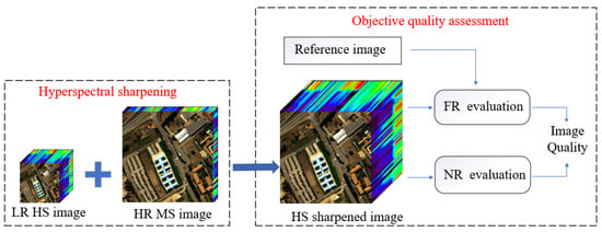
Figure 1.
The process of HS sharpening and objective quality assessment.
- Three statistical features following the standard Benford’s law are discovered from HS images. The features are the FDDs of (1) the singular values of low-frequency coefficients from discrete wavelet transform (DWT), (2) the complementary values of the high-frequency correlation between HS bands and MS bands, and (3) the information preservation coefficients between HS bands and MS bands at different resolution scales.
- An effective NR evaluation method for HS sharpened images via Benford’s law is proposed. The proposed method extracts the three FDD features from the HS sharpened images, then computes the distance between the extracted FDD features and the standard FDD feature, and finally obtains the evaluation results.
- Comprehensive experiments are conducted to verify the proposed method. The band assignment algorithm is applied to the four NR evaluation metrics of multispectral sharpening, and these adapted metrics are used to evaluate the HS sharpened images. Furthermore, the experiments adopt four commonly used FR evaluation metrics, three HS datasets, and 10 fusion methods to verify the accuracy and robustness of the proposed method.
The organizational structure of this paper is as follows: Section 2 briefly reviews related works. Section 3 provides a detailed introduction to the proposed method. Section 4 reports various experiments to validate the effectiveness of the proposed method. Section 5 discusses the performance of all related NR quality assessment metrics based on the experimental results and analysis. Finally, Section 6 concludes the paper.
2. Related Works
2.1. Wald’s Protocol
Lucien Wald et al. proposed the first protocol to quantitatively evaluate the quality of multispectral sharpening (often referred to as the Wald’s protocol) [51]. Wald’s protocol is a widely used remote sensing image fusion quality evaluation strategy. It was further discussed and established in [52,53]. The protocol mentions that the pansharpened images should have two properties: consistency and synthesis.
The consistency property is conducted at the observation resolution of imaging sensors. If an HR fused image is spatially degraded to the LR fused image by using the same modulation transfer function (MTF) as the original HS imaging sensor, then the image should be as consistent as possible with the original LR-HS image . The consistency can be represented as
where (A, B) represents the difference between two images A and B at a low spatial resolution, describes the error which should be small enough, i is the band index, and N is the number of bands in the HS image.
The synthesis property consists of two sub-properties. One states that the pansharpened image should be as identical as possible to the image acquired via the MS sensor if it had the high spatial resolution of the PAN sensor. In other words, the HR fused images should be as consistent as possible with the reference images . It can be represented as
where (A, B) represents the difference between two images A and B at the resolution level of the fused images, i.e., the full resolution scale.
The other sub-property states that the spectral vectors of the HR fused images and reference images should be as consistent as possible, which can be represented as
where (A, B) represents the distance between the spectral vectors of two images A and B at the resolution level of the fused image. The smaller the distance, the higher the spectral similarity.
2.2. FR Quality Assessment
FR quality assessment is a commonly used approach for evaluating the quality of fusion images. Currently, the mainstream of FR quality assessment follows the synthesis of the Wald’s protocol which requires higher resolution images as the references, although [54] mentioned that consistency can also be used as an evaluation strategy for FR. However, in practical applications, it is hard to obtain the images using higher spatial resolution imaging sensors. The reference image is not available. In FR quality assessment of image fusion, it is feasible to perform spatial degradation on all input images (PAN, MS, and HS images) in order to use the original HS or MS images as the references. FR assessment is therefore called reduced resolution assessment. Since the degraded fusion images can be directly compared with the reference images, FR evaluation results are usually considered more accurate and reliable. Most of the current quality assessments of HS sharpened images are almost always based on FR quality assessment [37].
The FR quality assessment of HS sharpening has been an open problem. Firstly, the reliability of FR assessment will decrease as the resolution scale differences increase [38], which often occurs in HS sharpening. Secondly, the difficulty in obtaining MTF-filter parameters during the degradation process is a potential influencing factor. Alternatively, some researchers use uniform filtering [31,32] and Gaussian filtering [29,30,36] to implement the spatial degradation. The size and the variance of Gaussian kernels used are different, making the accuracy of spatial degradation unreliable. Thirdly, due to the lack of benchmark HS datasets, the current way adopted by researchers is to simulate LR-HS and HR-MS images from the original HS images as the fusion inputs, and then use the original HS images as the reference for quality evaluation [38,55], which is inconsistent with the actual implementation of FR quality assessment.
2.3. NR Quality Assessment
NR quality assessment, also known as full resolution quality assessment, does not have a reference, but instead uses the input images, namely HR-PAN or HR-MS images, as the spatial or spectral references. NR assessment is more in line with practical evaluation processes. Although many NR evaluation methods designed for multispectral sharpening have been proposed, there is little dedicated NR quality assessment method for HS sharpened images. The most widespread NR evaluation metric is QNR [43]. It concerns two distortions: spatial distortion and spectral distortion. The spatial distortion is measured using the difference in the Q values between PAN and MS images at different scales, while the spectral distortion is measured using the change in the Q values among MS bands. There have been some variants and improvements originating from the QNR metric so far. These variants include FQNR [44], RQNR [45], HQNR [46], and GQNR [47], to name a few. Also, some other NR methods have been designed. The quality-estimation-by-fitting (QEF) method predicts the evaluation results via linear regression from the FR evaluation results at different degraded resolution scales [56]. Kalman QEF (KQEF) is subsequently designed to improve the QEF [57]. Moreover, the MVG-based QNR method (MQNR) extracts multiple spatial and spectral features from the fused images to build the distorted MVG model. The distance between the benchmark MVG model and the distorted MVG model is used to indicate the evaluation results [48]. With the help of large-scale datasets, deep-learning-based NR methods have also emerged and been used for PAN-MS fusion quality assessment [49].
Some researchers have attempted to apply NR quality assessment metrics of multispectral sharpening to evaluate HS sharpened images. In the practice of using PAN images to increase the spatial resolution of HS images, Javier et al. used drones, orthophotos, and satellite high spatial resolution data to enhance the resolution of airborne and satellite HS images. When conducting NR quality assessment, they calculated the spatial correlation coefficients (sCC) between each band of the fused HS image and the PAN image and averaged all sCC results as an evaluation of spatial quality. In addition, they computed the SAM between the degraded fused images and the original HS images to evaluate the spectral quality [58]. Meng et al. initially designed MQNR metric for the NR quality assessment of multispectral sharpening and applied the MQNR to HS sharpened images to verify its effectiveness [48]. In the cases of HS-MS image fusion, NR quality assessment is feasible in a band assignment way. The band assignment algorithm originated from HS-MS image fusion. According to the spectral overlap of MS and HS images, it divides the HS bands into multiple groups corresponding to each of MS bands, and then uses the pansharpening-based method to fuse the HS bands and MS images in each group [59]. Rocco et al. first applied the band assignment algorithm to NR quality assessment of HS sharpened images, when they conducted a study on HS sharpening using multiplatform data [15]. In NR quality evaluation, they proposed to assign each MS band to the related fused HS bands and obtained multiple MS-HS groups. Then, they adopted the spatial index of RQNR to evaluate the spatial quality of each group and the spectral index of FQNR to calculate the SAM between the degraded fused image and the original HS image. Another very interesting evaluation method is the task-based approach. Kawulok et al. retrieved the air pollution index, i.e., NO2 column from HS sharpened images and compared it with the ground-truth NO2 column to get the evaluation results [60]. Overall, although NR quality assessment faces more challenges than FR quality assessment, it is more practical and has less limitations.
2.4. Image Quality Assessment Based on Benford’s Law
Benford’s law is a numerical law. In 1881, Simon Newcomb discovered that the first few pages of the logarithmic table were more broken than the other pages, indicating a higher probability of the first digit being 1 in the values used for calculation [61]. Subsequently, Frank Benford rediscovered this phenomenon in 1935. After extensive testing and research, he found that as long as there were enough samples of data, the probability distribution of the first digit of the data followed a logarithmic criterion [62]. Benford’s law has received attention from people since then. At present, data from many fields in reality always indicate compliance with Benford’s law, such as mathematics [63], physics [64], social sciences [65], and environmental sciences [66]. Until today, Benford’s law still guides people to explore the principles behind it [67].
Ou et al. found that FDD features extracted from the discrete cosine transform (DCT) coefficients of natural images are highly sensitive to white noise, Gaussian blur, and fast fading, and applied Benford’s law to the quality assessment of natural images [68]. It has been verified in [69,70,71] that the high-frequency coefficients of discrete wavelet transform (DWT), shearlet coefficients, and singular values follow the standard Benford’s law. Therefore, the standard Benford’s law has been applied to distortion classification [69] and natural images quality assessment [70,71]. Additionally, the generalized Benford’s law [72] was used to evaluate the quality of natural images with external noise such as Gaussian white noise, JPEG compression distortion, blur distortion, etc. For the first time, Wu et al. introduced Benford’s law into the quality assessment of multispectral sharpening, who employed the extracted FDD feature of the angle components of the pansharpened images in the hyperspherical color domain to evaluate the spectral quality [50]. However, the method exhibits poor performance in evaluating HS sharpened images. Inspired by this, this paper proposes an NR method to evaluate the quality of HS sharpened images with the help of Benford’s law.
3. Proposed Method
Figure 2 shows the flowchart of the proposed method. The method consists of two parts. One part is the FDD feature extraction. The FDD features include a low-frequency FDD feature, a high-frequency FDD feature, and a Q-based FDD feature. The other part is the distance measurement, which calculates the difference between the distributions: the extracted FDD features and the FDD feature of the standard Benford’s law. A detailed introduction to each part of the proposed method will be provided in this section.
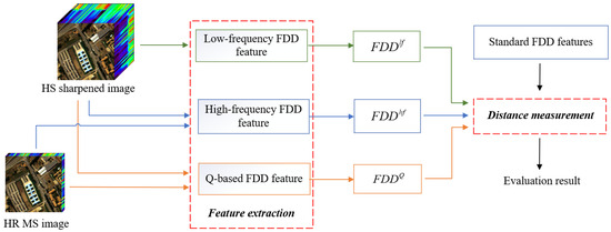
Figure 2.
Flowchart of the proposed method.
3.1. Standard Benford’s Law
The standard Benford’s law records the distribution probability of the first digits about a certain type of data. The first digit refers to the first non-zero digit of a numerical value from left to right. For example, the first digit of 2.45 is 2 and the first digit of −0.32 is 3. The standard Benford’s law is based on this numerical law, which holds that the distribution of the first digits of a large amount of data about a certain thing follows a logarithmic distribution. It can be described using the following:
where records the FDD feature of the first digit being n. The standard Benford’s law can be represented by a nine dimensional FDD feature, i.e., [P(1), P(2), …, P(9)]. The standard FDD feature is denoted as FDDstd in (5) and the first digit distribution is plotted in Figure 3.
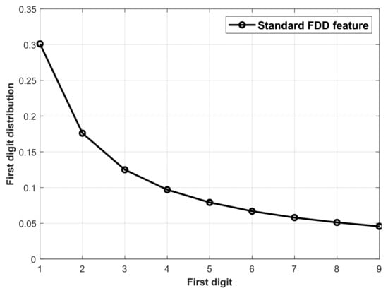
Figure 3.
The distribution of the FDDstd.
It is assumed that the FDD features extracted from the ideal fusion products should conform to the standard Benford’s law as much as possible, so that the standard FDD feature FDDstd can be used as the reference model. Fortunately, three quality perception features in high-quality HS image data are found. Through extensive experiments, it is verified that the features comply with the standard Benford’s law and are sensitive to distortions in HS sharpened images.
3.2. Quality Perception Features
HS images often have dozens or hundreds of spectral bands, which contain a large amount of information and have complex potential statistical characteristics. With the help of Benford’s law, it is possible to identify some stable features extracted from the HS images for quality assessment. After extensive experiments, three types of FDD features are found out, including a low-frequency FDD feature, a high-frequency FDD feature, and a Q-based FDD feature, which can effectively perceive the distortions of fusion results. A detailed description of the three types of FDD features is provided below.
3.2.1. Low-Frequency FDD Feature
Singular value decomposition has been widely used in image denoising in which the degree of image distortion is determined by detecting singular values. Moreover, the compact support property of Meyer wavelets makes them important and valuable in signal processing, image reconstruction, and analysis of distribution functions [73]. Motivated by this, this work tries to find the representative statistical features to characterize the quality of the HS images. Through lots of experiments on HS images, it is found that the FDD features of the singular values of the low-frequency coefficients within Meyer wavelet domain follow the standard Benford’s law. Firstly, Meyer wavelet transform is performed on each band of the HS image to obtain the low-frequency coefficients of the approximation images. Then, singular value decomposition is used so the coefficients and the singular values of all HS bands are obtained. Finally, the low-frequency FDD (denoted as FDDlf) feature is calculated based on the singular values.
To verify the effectiveness of the low-frequency FDD feature, experiments of the feature extraction are conducted on three different HS datasets, i.e., Pavia University dataset, Salinas dataset, and Cuprite dataset (see the detailed information of the datasets in Section 4.1). Figure 4 displays the distribution of the three FDDlf features from the datasets and the distribution of the FDDstd. Table 1 reports the specific values of the FDDstd and FDDlf features.
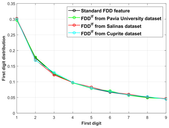
Figure 4.
The distributions of the FDDstd and FDDlf features from three HS datasets.

Table 1.
The specific values of the FDDstd and FDDlf features from three HS datasets. The first column represents the sources of the extracted FDDlf features and the FDDstd. P(n) records the FDDstd and FDDlf features of the first digit being n. The last column provides the symmetric Kullback–Leibler divergence (sKL) between the FDDstd and FDDlf features.
To compare the difference between the FDD features, symmetric Kullback–Leibler divergence (sKL) is used to measure the distance between the FDDstd and FDDlf. The calculation formula for sKL is as follows:
where A and B are the first digit distributions to be measured and Kullback–Leibler (KL) divergence is given by
From the values in Table 1, it can be seen that the sKL divergence between the FDDlf features and the FDDstd are close to 10−4. The distance between two probability distributions is very small. Based on the observations of Figure 4 and Table 1, it can be concluded that the FDDlf feature of the original HS images conform to the standard Benford’s law. This makes it possible to evaluate the quality of HS sharpened images based on the low-frequency FDD feature.
In order to test the sensitivity of the FDDlf feature to the quality of distorted HS images, two experiments are conducted on the HS datasets. In the first experiment, different types of noise are added to the datasets separately. The noises include Gaussian white noise with a mean of 0 and a gradually increasing standard deviation, Gaussian blur noise with a gradually increasing standard deviation, and multiplicative noise with a gradually increasing standard deviation. In the second experiment, four HS sharpened images, i.e., IR-TenSR [32], UTV [31], SFIM [20], MAP-SMM [24], and EXP (i.e., the upsampled image by cubic interpolation) with increasing fusion distortions are selected. Then, the FDDlf features are extracted from these distorted images and the FDDstd is used as the benchmark for distance measurement. Taking the experiment on the Pavia University dataset as an example, Figure 5 shows the distribution of the FDDlf features from the different distorted images and Table 2 gives the values of the FDDlf features from the HS sharpened images.
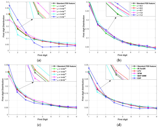
Figure 5.
The distributions of the FDDlf features from different distorted images of the Pavia University dataset: (a) images distorted by Gaussian white noise with gradually increasing standard deviation; (b) images distorted by Gaussian blur noise with gradually increasing standard deviation; (c) images distorted by multiplicative noise with gradually increasing standard deviation; (d) HS sharpened images with increasing fusion distortion.

Table 2.
The specific values of the FDDstd and FDDlf features from different fused images of the Pavia University dataset.
From Figure 5a–c, it can be seen that for different types of external noise, as the noise increases, the FDDlf features of the distorted images further deviate from the FDDstd, indicating that the FDDlf features exhibit good performance in measuring external noise. In Figure 5d and Table 2, the FDDlf features of the different fused images and EXP image with increasing fusion distortion are presented. Table 2 shows that as the degree of fusion distortion increases, the values of sKL divergence also monotonically increase. This phenomenon can also be observed in Figure 5d. The two experiments demonstrate that the FDDlf feature can be selected as a quality perception feature to evaluate the quality of HS sharpened images.
3.2.2. High-Frequency FDD Feature
For the quality evaluation of natural images, the FDD features extracted from high-frequency coefficients of DWT, DCT, and shearlet have been proven to be effective [69,70,71]. Unfortunately, these typical FDD features are ineffective for hyperspectral images and cannot be used for quality evaluation of HS sharpened images. This is because the distortion of natural images often comes from external noise, such as image transmission, image compression, etc. The distortion of fused images, as an internal distortion, is generated in the fusion process. Therefore, the FDD features of natural images may view fusion distortion as the structure of the image itself, rather than distortion. To tackle with this problem, a new way is designed to obtain an effective high-frequency FDD feature as a quality perception feature.
- (1)
- The band assignment on the fused HS image and the HR-MS image is performed according to [59]. Suppose the original HS image of N bands and the HR-MS image of M bands are fused, the HS sharpened image will have N bands. After band assignment, M groups can be obtained so that each group contains one MS band and several corresponding HS bands. Then, the quality assessment of HS sharpened image can be treated as a combination of multiple pansharpening quality assessment cases.
- (2)
- For each group, the high-frequency components are extracted from the HS bands and the MS band, respectively. The extraction process of the high-frequency component of HS/MS band is as follows:
Next, the high-frequency components of HS/MS bands are divided into non-overlapping blocks and the correlation coefficients between the blocks of each HS band and the MS band are calculated. The complementary values of the correlation coefficients are calculated as
where is the high-frequency difference matrix between the ith fused HS band and the MS band in the kth group, is the high-frequency component of the ith fused HS band in the kth group, and is the high-frequency component of the MS band in the same group. ) is the calculation of correlation coefficients in blocks, T is the number of HS bands in kth group, and M is the number of the groups. The set of all high-frequency difference matrices is denoted as . The lower the high-frequency similarity between two bands, the higher the values of , which facilitates the detection of the spatial distortion in the HS sharpened images.
- (3)
- The high-frequency FDD feature, denoted as FDDhf is obtained by counting the number of the first digit of .
Similar to Section 3.2.1, the high-frequency FDD feature is experimentally verified to comply with the standard Benford’s law (The detailed information of the fused HS image and HR-MS image in the experiment are provided in Section 4.1). Then, FDDhf features from three HS datasets are extracted separately and compared with the FDDstd. The FDDhf features of three HS datasets are presented in Figure 6 and Table 3. It can be seen that the values of sKL are very small reaching the order of 10−3 or 10−4, and the curves of the FDDhf features match well with the FDDstd. The experimental results demonstrate that the FDDhf can serve as a stable high-frequency feature representing the quality of HS images.
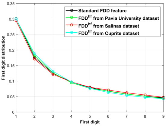
Figure 6.
The distributions of the FDDstd and FDDhf features from three HS datasets.

Table 3.
The specified values of the FDDstd and the FDDhf features from three HS datasets.
Furthermore, FDDhf features are extracted from four different fused images and EXP on three HS datasets. Figure 7 and Table 4 show the experimental results on the Pavia University dataset. In Figure 7, it can be seen that the FDDhf features of different fused images significantly deviate from the FDDstd and the FDDhf feature of EXP appears the maximum deviation. From the values of sKL in Table 4, it can be seen that as the distortion of the fused image increases, the values of the FDDhf features also increase and the trend of the change is consistent. The experiment demonstrates that the high-frequency FDD feature is an appropriate quality perception feature for HS images and has the ability to detect fusion distortion.
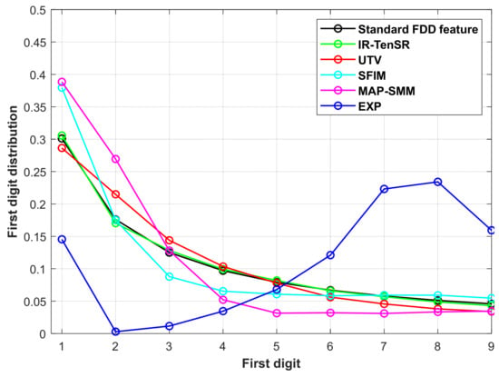
Figure 7.
The distributions of the FDDstd and FDDhf features from the fused images of the Pavia University dataset.

Table 4.
The specific values of the FDDstd and FDDhf features from the fused images of the Pavia University dataset.
3.2.3. Q-Based FDD Feature
Since the Q index was proposed by Wang et al. in 2002 [74], it has demonstrated a powerful ability to measure the similarity between two images. Several variations of the Q-based QNRs, such as FQNR, RQNR, and HQNR, are the most commonly used in NR-quality assessment of multispectral sharpening. Motivated by this, it is meaningful to find a Q-based FDD feature satisfying the assumption of the preservation of the statistical Q through the hyperspectral sharpening process.
- (1)
- Similar to Section 3.2.2, the band assignment is performed to the HS sharpened image and the HR-MS image and M groups are obtained. In each group, there are one MS band and several HS bands.
- (2)
- For each group, the Q values between the MS and HS bands at different resolution scales are calculated. For a certain resolution scale, the Q values are calculated as [74]
- (3)
- The Q-based FDD feature, denoted as FDDQ, is obtained by counting the number of the first digit on the matrix.
Also, the experiment on the Pavia University dataset is taken as an example to show the experimental validation. Considering the different spatial resolutions of LR-HS images and HR-MS images in practice, the original HS image is degraded at five different resolution scales and the degradation ratios are 2, 4, 6, 8, and 10. At each resolution scale, the corresponding Q-based FDD features are extracted, i.e., , , , , and . The experiment results are shown in Figure 8 and Table 5. It can be seen that the Q-based FDD features at different scales have stable values around 10−3 and basically match with the standard FDD feature. Therefore, for HR-MS and LR-HS images with different spatial resolution ratios in practice, the FDDQ can be used as a feature to represent the quality of HS images.
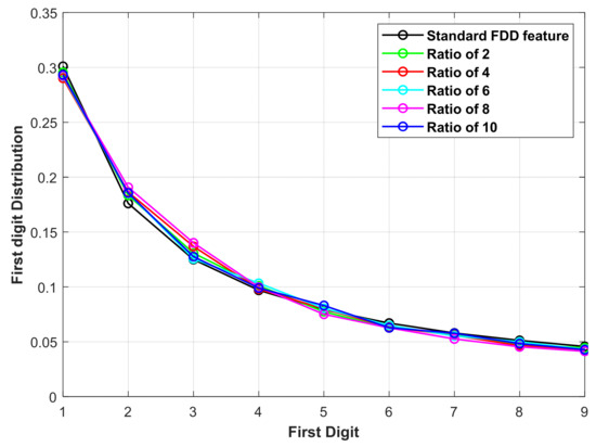
Figure 8.
The distributions of the FDDstd and FDDQ features from the Pavia University dataset at different resolution ratios.

Table 5.
The specific values of the FDDstd and FDDQ features from the Pavia University dataset at different resolution ratios.
Taking the as an example, the Q-based FDD features from four fused images are extracted. Figure 9 and Table 6 show their distributions and specific values. It can be seen that the Q-based FDD feature of IR-TenSR with lower distortion are closer to the standard FDD feature. Due to the more severe fusion distortion of SFIM, MAP-SMM, and EXP, their Q-based FDD features deviate further from the standard FDD feature. Therefore, the Q-based FDD feature can effectively perceive fusion distortion.
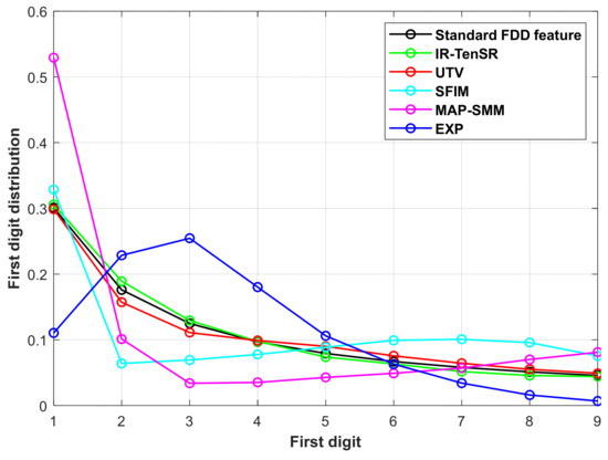
Figure 9.
The distributions of the FDDstd and FDDQ features from the fused images of the Pavia University dataset.

Table 6.
The specific values of the FDDstd and FDDQ features from the fused images of the Pavia University dataset.
3.3. Distance Measurement
In the above experiments, three quality perception features for HS sharpening have been identified and validated on different fused images of different HS datasets. Three quality perception features are the low-frequency FDD feature FDDlf, the high-frequency FDD feature FDDhf, and the Q-based FDD feature FDDQ. The features measure the fusion distortion from different perspectives. Therefore, it is necessary to integrate them in order to comprehensively evaluate the quality of HS sharpened images. Here, the standard FDD feature FDDstd is taken as the benchmark for distance measurement. Specifically, Manhattan distance is used to measure the distance between the distorted FDD features and the standard FDD feature. The distance measurement is calculated as
The ideal value of is 1, and the larger the value, the higher the quality of the HS sharpened image.
4. Experiments
4.1. Datasets
In the experiments, three typical HS datasets, i.e., Pavia University dataset [55], Salinas dataset [9], and Cuprite dataset [55] are selected.
- The Pavia University dataset was collected using German Reflective Optics Spectrographic Imaging System (ROSIS-03) sensors and recorded partial scenes of Pavia city, Italy. The dataset contains 103 available bands, covering a spectral range of 0.43–0.86 μm. The dimension is 610 × 340 pixels with a spatial resolution of 1.3 m.
- The Salinas dataset was captured using the AVIRIS sensor of NASA and recorded parts of the Salinas Valley in California. The dataset has 204 available bands and covers a spectral range of 0.4–2.5 μm. The spatial resolution of the HS images is 3.7 m with the dimension of 512 × 217 pixels.
- The Cuprite dataset was also collected using the AVIRIS sensor and recorded parts of the Cuprite area in Nevada. The original dataset contains 224 bands and the spectral range covers from 0.37–2.48 μm. The bad bands with low signal-to-noise are removed and 185 bands are retained for the experiment. The dimension of the HS images is 512 × 612 pixels with a spatial resolution of 20 m.
To generate LR-HS and HR-MS images for HS-MS fusion, spatial and spectral simulations are conducted on these HS datasets. The simulation process is the same as that in [55]. Specifically, spatial filtering is performed on the original HS image to obtain the LR-HS image. The convolutional kernel of the spatial filtering is a 7 × 7 Gaussian kernel with zero-mean and a standard deviation of 3. The spatial resolution of the obtained LR-HS image is 1/4 of the original HS image. To obtain HR-MS image, the spectral response functions of the IKONOS sensor and the WorldView3 sensor are used as the spectral filters. The spectral coverage range of the IKONOS sensor is 0.45–0.9 μm [55], while the spectral coverage range of the Worldview3 sensor is 0.4–2.365 μm [15]. Therefore, the Pavia University dataset is filtered using the spectral response function of IKONOS and HR-MS image with four bands is obtained. Similarly, the Salinas dataset and Cuprite dataset are filtered using the spectral response function of WorldView3 and HR-MS images with 16 bands are obtained.
4.2. HS Sharpening Methods
Among the four categories of fusion methods mentioned in Section 1, ten HS sharpening methods are selected.
- Classical pansharpening-based methods. Four methods, including PCA [17], GSA [18], GLP [19], and SFIM [20] have been selected. PCA and GSA are typical CS-based fusion methods, which are built on principal component transformation and Gram-Schmidt orthogonal transformation, respectively. They have been widely used in many practical applications. GLP and SFIM are representative MRA-based fusion methods, which improve the spatial resolution of LR images by injecting the spatial details obtained through spatial filtering. After the band assignment, these methods can be applied to fuse HS images, since HS sharpening can be seen as a multi pansharpening cases.
- MF-based methods. Two methods, MAP-SMM [24] and HySure [25], have been selected. MAP-SMM utilizes a stochastic mixing model to estimate the underlying spectral scene content and develops a cost function to optimize the estimated HS data relative to the input HS/MS images. HySure formulates the HS sharpening as the minimization of a convex objective function with respect to subspace coefficients.
- TR-based methods. Three methods, including LTMR [29], UTV [31], and IR-TenSR [32] have been selected. LTMR learns the spectral subspace from the LR-HS image via singular value decomposition, and then estimates the coefficients via the low tensor multi-rank prior. UTV utilizes the classical Tucker decomposition to decompose the target HR-HS image as a sparse core tensor multiplied by the dictionary matrices along with the three modes. Then it conducts proximal alternating optimization scheme and the alternating direction method of multipliers to iteratively solve the proposed model. IR-TenSR integrates the global spectral–spatial low-rank and the nonlocal self-similarity priors of HR-HS image. Then it uses an iterative regularization procedure and develops an algorithm based on the proximal alternating minimization method to solve the proposed model.
- Deep CNN-based method. CNN-Fus method [33] is selected for experiment. CNN-Fus learns the subspace from LR-HS image via singular value decomposition. Then it approximates the desired HR-HS image with the low-dimensional subspace multiplied by the coefficients. It uses the well-trained CNN designed for gray image denoising to regularize the estimation of coefficients.
4.3. Quality Assessment Metrics
To evaluate the quality of HS sharpened images, four FR metrics are selected: PSNR [38], SAM [39], ERGAS [40], and Q2n [42]. PSNR evaluates the spatial reconstruction quality, SAM is the metric for evaluating angular distortion of spectra, and ERGAS and Q2n measure the overall distortion. Furthermore, the proposed method is compared with four NR evaluation metrics including QNR [43], FQNR [44], RQNR [45], and MQNR [48]. As mentioned in Section 3.2.2, after applying the band assignment to the HS and MS bands, the evaluation of the fused images can be seen as a combination of multiple pansharpening evaluation cases. To obtain the final evaluation results, these NR metrics are performed to HS sharpened images in each group and the evaluations of all groups are averaged. In addition, the spatial distortion indexes and spectral distortion indexes of the NR metrics are analyzed in Section 4.5.4. The spatial distortion index and spectral distortion index of QNR are respectively denoted as and . Similarly, and are the spatial and spectral indexes of FQNR, and are the spatial and spectral indexes of MQNR. is the spatial index of RQNR.
To analyze the reliability and accuracy of all NR metrics, the evaluation results of FR metrics are used as the testing benchmark. In other words, if the result of an NR metric is consistent with the results of FR metrics, then the NR metric is considered accurate. Pearson linear correlation coefficient (PLCC) [71], Spearman rank-order correlation coefficient (SROCC) [71], and Kendall rank-order correlation coefficient (KROCC) [71] are used to calculate the correlation between the results of NR metrics and the benchmark. PLCC reflects the evaluation accuracy of the NR metrics. SROCC and KROCC are used to reflect the evaluation monotonicity of the NR metrics. Better performance should provide higher PLCC, SROCC, and KROCC values.
4.4. Experiment Environment
To ensure a fair comparison, all experiments in this paper are coded on MATLAB 2021a, using a laptop equipped with memory of 16.0 GB RAM, AMD Ryzen 7 6800H CPU, Radeon Graphics, and NVIDIA GeForce RTX 3060 GPU.
4.5. Experimental Results and Analysis
4.5.1. Subjective Evaluation
Figure 10, Figure 11 and Figure 12 respectively show the sub scenes in the fusion results of the Pavia University, Salinas, and Cuprite HS datasets. Although it is difficult to visually analyze the results of HS sharpening due to hundreds of HS bands, spectral filtering is performed on the fused HS images to obtain MS images, and then select the red, green, and blue bands for true color composite display. The zoomed view of a local area is displayed in the upper right. The corresponding RMSE heat maps are also provided below each fused image.
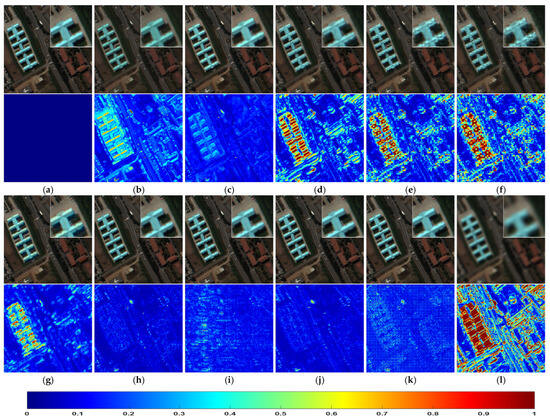
Figure 10.
Fused images of different HS sharpening methods on Pavia University dataset: (a) REF; (b) PCA; (c) GSA; (d) GLP; (e) SFIM; (f) MAP-SMM; (g) HySure; (h) LTMR; (i) UTV; (j) IR-TenSR; (k) CNN-Fus; (l) EXP.
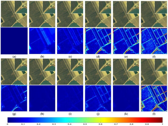
Figure 11.
Fused images of different HS sharpening fusion methods on Salinas dataset: (a) REF; (b) PCA; (c) GSA; (d) GLP; (e) SFIM; (f) MAP-SMM; (g) HySure; (h) LTMR; (i) UTV; (j) IR-TenSR; (k) CNN-Fus; (l) EXP.
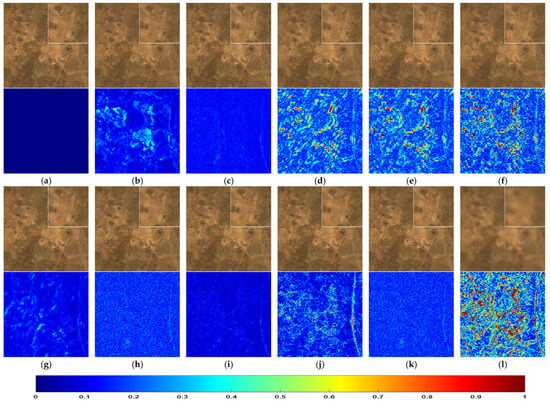
Figure 12.
Fused images of different HS sharpening methods on Cuprite dataset: (a) REF; (b) PCA; (c) GSA; (d) GLP; (e) SFIM; (f) MAP-SMM; (g) HySure; (h) LTMR; (i) UTV; (j) IR-TenSR; (k) CNN-Fus; (l) EXP.
For the Pavia University dataset, it can be seen from the true color images in Figure 10 that SFIM and MAP-SMM images have obvious blocking distortion, EXP appears too blurry, and other fused images have better visual effects. The RMSE heat maps can help us easily distinguish the subtle visual difference among the fused results. The images in Figure 10h,j show that LTMR and IR-TenSR have the minimal spatial distortion. GSA, a traditional pansharpening method, has also achieved good fusion result. GLP, SFIM, MAP-SMM show the poor results as the significant distortions spread uniformly in the whole scene.
For the Salinas dataset, the fused images and their RMSE heat maps are presented in Figure 11. Figure 11 shows a farmland scene, mostly in flat areas. From the zoomed windows, it can be seen that the TR-based methods and deep CNN-based method, i.e., LTMR, UTV, IR-TenSR, and CNN-Fus are very similar to Figure 11a, the reference image. Moreover, Figure 11d–g exhibit apparent block distortions, especially in SFIM and MAP-SMM images. From the heat maps, it can be observed that the CNN-Fus, LTMR, and UTV methods have achieved excellent fusion results. GLP, SFIM and MAP-SMM still show poor results, especially around the roads.
Figure 12 shows the fusion results and RMSE heat maps on the Cuprite dataset. There are almost no man-made buildings or vegetations in the scene and the types of ground objects are relatively single. Despite of the low spatial resolution of the dataset, most fusion methods still achieve good fusion results, making it difficult to distinguish the differences in true color images. With the help of the RMSE heat maps, it can be seen that GSA and UTV have the smallest error, LTMR and CNN-Fus achieve suboptimal results, and GLP, SFIM, and MAPSMM methods are still the poorest. It is worth mentioning that, due to the hundreds of bands in HS sharpened images, it is difficult to distinguish spectral distortion accurately from the true color images only.
4.5.2. FR and NR Evaluations
The LR-HS and HR-MS images (mentioned in Section 4.1) are fused to obtain the fused images. Then all fusion products are evaluated using four FR metrics and five NR metrics and the experimental results are presented in Table 7, Table 8, Table 9 and Figure 13, Figure 14 and Figure 15. For FR evaluation, the original HS images are taken as the reference and four FR metrics are used to evaluate. For NR evaluation, band assignment is conducted on the fused images and the HR-MS images to get multiple groups. Each group contains one MS band and several HS bands.

Table 7.
The FR and NR evaluation results of the fused images on Pavia University dataset (best results are in bold and the second-best results are underlined).

Table 8.
The FR and NR evaluation results of the fused images on Salinas dataset (best results are in bold and the second-best results are underlined).

Table 9.
The FR and NR evaluation results of the fused images on Cuprite dataset (best results are in bold and the second-best results are underlined).

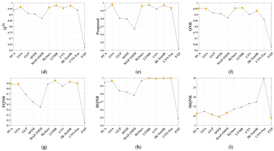
Figure 13.
The evaluation values of FR and NR metrics on Pavia University dataset: (a) PSNR; (b) SAM; (c) ERGAS; (d) Q2n; (e) Proposed; (f) QNR; (g) FQNR; (h) RQNR; (i) MQNR.
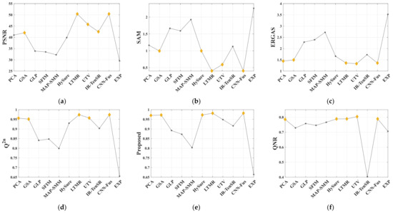

Figure 14.
The evaluation values of FR and NR metrics on Salinas dataset: (a) PSNR; (b) SAM; (c) ERGAS; (d) Q2n; (e) Proposed; (f) QNR; (g) FQNR; (h) RQNR; (i) MQNR.
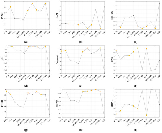
Figure 15.
The evaluation values of FR and NR metrics on Cuprite dataset: (a) PSNR; (b) SAM; (c) ERGAS; (d) Q2n; (e) Proposed; (f) QNR; (g) FQNR; (h) RQNR; (i) MQNR.
Each group is evaluated using NR metrics and the final NR evaluation results are obtained by averaging the NR evaluation results of each group. Table 7, Table 8, Table 9 report the FR and NR evaluation results of the fused images on three HS datasets. For each metric, the best result is marked in bold, and the second-best result is underlined. For a more intuitive comparison, the evaluation results of each metric are displayed in a line graph. Figure 13, Figure 14 and Figure 15 are the line graphs for different datasets, in which the best five results are marked with yellow blocks.
From the results in Table 7, it can be seen that LTMR and IR-TenSR achieve the best or second-best results among FR metrics, and EXP has the worst results in terms of FR metrics. For Table 8 and Table 9, CNN-Fus and LTMR are always the best or second-best among FR metrics while EXP is the worst. This phenomenon is basically consistent with the subjective analysis results in Figure 10, Figure 11 and Figure 12. From Figure 13, Figure 14 and Figure 15, it can be seen that there are some correlations among the four curves of FR metrics, such as the optimal evaluation results among them basically including GSA, LTMR, UTV, and CNN-Fus. In the performance of NR metrics, the trend of the proposed method is very similar to Q2n and ERGAS, indicating that the proposed method has shown excellent performance in evaluating overall quality. FQNR and RQNR also have a similar trend to the Q2n curves, but their evaluations are not accurate in methods with good fusion results. For example, in the evaluations of LTMR, UTV, IR-TenSR, and CNN-Fus, the yellow blocks in RQNR are very close. For QNR, it has good evaluation ability on the Pavia University dataset, but its evaluation performance significantly decreases on the other two datasets, as its curves are clearly unrelated. The curves of MQNR are inconsistent with those of FR metric, which means it cannot be used for accurate evaluation. In addition, the evaluation results of the NR metrics have a certain correlation with PSNR and SAM, but the correlations are not stable enough, especially on the Cuprite dataset.
4.5.3. The Consistency between FR and NR Metrics
FR quality assessment is commonly considered more reliable than NR evaluation, since the reference is available and used in FR. Therefore, it is reasonable to use the evaluation conclusion of FR as a reliability and accuracy benchmark for validating NR metrics. In order to verify the consistency between FR and NR metrics and analyze the differences, consistency experiments are conducted in which the evaluation results of Q2n, SAM, and PSNR are considered as representatives of overall quality, spectral quality, and spatial quality, respectively. Then the PLCC, SROCC, and KROCC are calculated between all NR metrics and Q2n, SAM, and PSNR separately. Table 10, Table 11 and Table 12 report the correlations on three datasets. The higher the values, the more consistent with the FR evaluation. The negative values indicate that the evaluation results of the two metrics have opposite trend. For a more intuitive analysis, the correlations are plotted in the form of a bar graph in Figure 16, Figure 17 and Figure 18, in which the negative values are set to 0.

Table 10.
PLCC, SROCC, and KROCC between Q2n and all NR metrics on three HS datasets (best results are in bold and the second-best results are underlined).

Table 11.
PLCC, SROCC, and KROCC between SAM and all NR metrics on three HS datasets (best results are in bold and the second-best results are underlined).

Table 12.
PLCC, SROCC and KROCC between PSNR and all NR metrics on three HS datasets (best results are in bold and the second-best results are underlined).

Figure 16.
PLCC, SROCC, and KROCC between all NR metrics and Q2n on three HS datasets: (a) Pavia University dataset; (b) Salinas dataset; (c) Cuprite dataset.

Figure 17.
PLCC, SROCC, and KROCC between all NR metrics and SAM on three HS datasets: (a) Pavia University dataset; (b) Salinas dataset; (c) Cuprite dataset.

Figure 18.
PLCC, SROCC, and KROCC between all NR metrics and PSNR on three HS datasets: (a) Pavia University dataset; (b) Salinas dataset; (c) Cuprite dataset.
Table 10 and Figure 16 show the correlations between NR metrics and Q2n for evaluating the overall quality. It can be seen that the proposed method has the highest or second-highest correlations with the evaluation results of Q2n on all three datasets. On the Cuprite dataset, there is a significant decrease in the accuracy of the other NR metrics, while the proposed method still maintains excellent evaluation performance. For the FQNR and RQNR metrics, they can only perform the good evaluation performance on a single dataset and show unstable evaluation performance and weak robustness. For the QNR and MQNR metrics, their evaluation results show a weaker correlation or even negative values compared to Q2n, which indicates the two NR metrics are not reliable to evaluate the overall quality.
For the spectral quality evaluation, Table 11 and Figure 17 show the correlations between NR metrics and SAM metric. In Table 11, it can be seen that the proposed method stays in a stable first tier on all datasets and has good robustness, especially on the Cuprite dataset. In contrast, the negative values appear in the other NR metrics, which indicates the metrics cannot accurately evaluate the spectral quality of the Cuprite dataset. Although RQNR achieves the second-best in terms of KROCC, its numerical value (0.0545) is much smaller than the proposed method (0.345). On the Salinas dataset, FQNR is the most relevant to SAM in terms of PLCC and SRCC. However, FQNR performs poorly on the other two datasets. This is similar to its situation in Table 10. QNR shows good correlation on the Pavia University dataset but is unstable on the other datasets.
For the spatial distortion evaluation, Table 12 and Figure 18 show the correlations between NR metrics and PSNR. FQNR and RQNR achieve the highest correlation with PSNR on datasets Pavia University and Salinas. The proposed method is closer to PSNR than other metrics on the Cuprite dataset. The reason is that Benford’s law is based on the statistical characteristics of data, making it more sensitive to large-scale spatial features (i.e., lower spatial resolution). The Cuprite dataset has a spatial resolution of 20 m, which is much lower than the other datasets. Therefore, FQNR and RQNR metrics designed specifically for high spatial resolution (i.e., the multispectral sharpening) are more effective in perceiving small-scale spatial features. Additionally, it can be observed in Table 12 that the values of the proposed method are close to FQNR and RQNR on the Pavia University and Salinas datasets and exhibit stability.
From the consistency experiment results, the following conclusions can be drawn: (1) Compared with the other NR metrics, the evaluation results of the proposed method are generally closer to those of FR on all datasets. (2) The proposed method achieves the best results on the Cuprite dataset. (3) Compared with the other NR metrics, the proposed method is more stable and robust for different datasets. (4) QNR and MQNR metrics differ significantly from FR, making the quality evaluation of HS sharpened images unreliable.
Overall, the proposed method exhibits optimal performance in evaluating global and spectral quality and has high robustness. The FQNR and RQNR can only exhibit optimal performance on one to two datasets and have poor robustness. QNR and MQNR are not suitable for NR quality assessment of HS sharpened images.
4.5.4. Analysis of the Sub-Index in NR Metrics
In order to investigate the performance of FDDlf, FDDhf, and FDDQ, the sub-indexes of all NR metrics are analyzed and compared by calculating the SROCC between the spectral/spatial distortion index and all FR metrics. SROCC is often used to reflect the effectiveness of the spatial/spectral indexes. The higher the SROCC, the more accurate the ranking of the evaluation results of the sub-index, and the more effective the sub-index is. Table 13, Table 14 and Table 15 report the SROCC results between all spatial/spectral indexes and all FR metrics. The rows on top represent the spatial indexes of the NR metrics, the rows in the middle represent the spectral indexes of the NR metrics, and the bottom seven rows belong to the sub-indexes proposed in this paper. PSNR reflects the ability to measure the spatial distortion, SAM presents the ability to measure the angular distortion of the spectrum, and ERGAS and Q2n reflect the performance of measuring the overall quality.

Table 13.
SROCC between sub-indexes and all FR metrics on Pavia University dataset (best results are in bold and the second-best results are underlined).

Table 14.
SROCC between sub-indexes and all FR metrics on Salinas dataset (best results are in bold and the second-best results are underlined).

Table 15.
SROCC between sub-indexes and all FR metrics on Cuprite dataset (best results are in bold and the second-best results are underlined).
For the spatial indexes, it can be seen that achieves the highest SROCC with PSNR on the first and second dataset, while obtains optimal performance on the second and third dataset. The SROCC of are the lowest among all spatial indexes. Moreover, the NR spatial indexes also demonstrate high accuracy in measuring overall distortion, such as the performance of on the first dataset and on the second dataset, although their performances are not stable on all datasets. In addition, these NR indexes are not accurate in measuring the spectral distortion, since they show negative SROCC values on the Cuprite dataset.
For the spectral indexes, achieves the best performance among the three NR spectral indexes, and it also demonstrates excellent performance in measuring the spatial and overall distortion on all three datasets. All SROCCs of and are negative, indicating that they fail to measure fusion distortion. The reason may be that the assumption of invariance in the relationship between HS bands is unreasonable. For example, the spectral distortion of EXP is considered smallest in pansharpening and the results of both SAM and should be close to 0. In HS sharpening, however, the SAM values of EXP are always the worst and the results of are still close to 0. The completely opposite evaluation results of SAM and lead to poor performance of . For , as it inherits the assumption of QNR’s spectral distortion index, the results of are also unreliable.
For the sub-indexes proposed, each of the FDD features and their pairwise combinations are compared separately with FR metrics. It can be seen that the best evaluation performance is not achieved by using all three FDD features. The performance of different types of FDD features varies on different datasets. FDDhf and FDDQ both have stable evaluation performance, and combining them can obtain more accurate and stable evaluation results. In contrast, the ability of FDDlf to measure various distortions is weak since FDDlf only characterize the statistics of the fused image itself, without considering the relationship between the fused image and the input images (HR-MS and LR-HS). Due to the excellent performance of FDDlf in measuring external distortion, it is retained in QFDD to enhance the robustness of the proposed method. Overall, from the data in the tables, it can be seen that the sub-indexes of the proposed method exhibit high accuracy and excellent robustness in measuring various distortions, especially global distortion. The proposed method is effective to measure the overall distortion of HS sharpened image.
5. Discussion
5.1. The Distortions in HS Sharpening
For HS sharpening (or MS sharpening), the input images have already been denoised and registered. In other words, the input images have no noises like stripe noise, Gaussian white noise, salt and pepper noise, etc. Similar to the authentic distortions of natural images, the distortions in HS sharpening are inherent in the fused image itself and some external distortions are not considered. Therefore, the quality assessment should pay more attention to the distortions yielded in HS sharpening process. To date, the fusion community consensus is that there exist two types of distortions, i.e., the spatial distortion and the spectral distortion. However, due to the large number of spectral bands in HS sharpened images, it is difficult to separate the spectral distortion and spatial distortion completely. In the experimental results, it can be seen that there exists, to some extent, a correlation between the evaluation results of spectral and spatial indexes. There is coupling between the two distortions. It is more reasonable to describe the overall quality of fusion. To define what the term (spatial/spectral) quality means and quantify the quality in a measurable way make the quality assessment of HS sharpening a complex task.
5.2. The Accuracy of NR Quality Assessment
For the quality assessment of HS sharpened images, the qualitative evaluation is infeasible. The subjective evaluation of HS sharpened bands within the visible spectrum has limitation. Therefore, it is very difficult to verify the accuracy of NR metrics using DMOS (difference mean opinion score) values obtained from subjective evaluation. Due to the rarity of the real reference images, NR quality assessment of the fused images is much debated, especially for NR evaluation of HS sharpened images at full resolution scale. If the ranking of different fusion results in an NR evaluation is consistent with the ranking based on full-reference evaluation, then the NR method is considered effective and reliable. This assumption is a feasible way in current situation. In this paper, experiments are conducted on the consistency between NR and FR metrics to test the accuracy of NR metrics. The experimental results show that the proposed method is generally closer to the evaluation results of FR compared to other NR metrics. However, for the datasets with high spatial resolution (i.e., Pavia University and Salinas), the proposed method does not have significant advantages. FQNR and RQNR metrics have good accuracy in measuring overall and spatial quality on the Pavia University and Salinas datasets but have poor performance on the Cuprite dataset with low spatial resolution, which indicates the metrics are sensitive to the spatial resolution of HS sharpened images and have weak robustness. Compared to FR, QNR and MQNR show opposite evaluation results, so they are not suitable for evaluating HS sharpening.
5.3. The Limitations
Although the proposed method is tested by using three different HS datasets, there still may be potential limitations: (1) The input images (i.e., HR-MS and LR-HS images) used when generating fusion results are simulated from the HS dataset itself. The effectiveness of the proposed method is uncertain about heterogeneous or multi-platform HS data. (2) The experimental results show that the proposed method has limitations in detecting the spatial distortion of the HS sharpened images with high spatial resolution. We believe that there is a potential connection between the spatial information of image and Benford’s law. The implicit relationship is worth exploring and will help design a more accurate metric.
6. Conclusions
This paper proposes a no-reference quality assessment method of HS sharpened images without the need for a reference image or any other simulations based on Wald’s protocol. The method designs three quality perception features, namely FDDlf, FDDhf, and FDDQ, to perceive the quality and employs the standard Benford’s law as a benchmark to evaluate the fusion distortion of HS sharpened images. The extensive experiments are conducted to verify the effectiveness of the proposed method. Compared with the other four commonly used NR metrics, the proposed method is more stable and robust for different HS datasets, although the performance of the FDD features varies on different datasets. In addition, the evaluation results of the proposed method are generally closer to those of FR on all HS datasets. The proposed method can be flexibly used for evaluating spectral, spatial, and overall distortion without relying on the type of sensors and scale of the dataset. To obtain a more accurate QFDD by applying the weights to the three FDD features should be the subject of future work.
Author Contributions
Conceptualization, X.L.; Data curation, J.W.; Formal analysis, X.H.; Funding acquisition, X.L.; Investigation, X.H.; Methodology, X.H. and X.L.; Project administration, B.W. and B.L.; Resources, X.L.; Software, X.H.; Supervision, X.L.; Validation, J.W. and B.W.; Visualization, X.H.; Writing—original draft, X.H.; Writing—review & editing, X.L., Y.S. and B.L. All authors have read and agreed to the published version of the manuscript.
Funding
This work is supported by the Practice and Innovation Funds for Graduate Students of Northwestern Polytechnical University, in part by the Key R&D Plan of Shaanxi Province (No. 2024GX-YBXM-054), and in part by the National Natural Science Foundation of China (No. 62001394).
Data Availability Statement
Data are contained within the article.
Conflicts of Interest
The authors declare no conflict of interest.
References
- Bai, L.; Dai, J.; Song, Y.; Liu, Z.; Chen, W.; Wang, N.; Wu, C. Predictive prospecting using remote sensing in a mountainous terrestrial volcanic area, in Western Bangongco–Nujiang Mineralization Belt, Tibet. Remote Sens. 2023, 15, 4851. [Google Scholar] [CrossRef]
- Zhou, Q.; Wang, S.; Guan, K. Advancing airborne hyperspectral data processing and applications for sustainable agriculture using RTM-based machine learning. In Proceedings of the IGARSS 2023–2023 IEEE International Geoscience and Remote Sensing Symposium, Pasadena, CA, USA, 16–21 July 2023. [Google Scholar]
- Li, H.; Zhou, B.; Xu, F. Variation analysis of spectral characteristics of reclamation vegetation in a rare earth mining area under environmental stress. IEEE Trans. Geosci. Remote Sens. 2022, 60, 4408412. [Google Scholar] [CrossRef]
- Zhang, Y.; Li, X.; Wei, B.; Li, L.; Yue, S. A Fast Hyperspectral Tracking Method via Channel Selection. Remote Sens. 2023, 15, 1557. [Google Scholar] [CrossRef]
- Xie, M.; Gu, M.; Zhang, C.; Hu, Y.; Yang, T.; Huang, P.; Li, H. Comparative study of the atmospheric gas composition detection capabilities of FY-3D/HIRAS-I and FY-3E/HIRAS-II based on information capacity. Remote Sens. 2023, 15, 4096. [Google Scholar] [CrossRef]
- Acito, N. Improved learning-based approach for atmospheric compensation of VNIR-SWIR hyperspectral data. IEEE Trans. Geosci. Remote Sens. 2022, 60, 5512715. [Google Scholar] [CrossRef]
- Wright, L.A.; Kindel, B.C.; Pilewskie, P.; Leisso, N.P.; Kampe, T.U.; Schmidt, K.S. Below-cloud atmospheric correction of airborne hyperspectral imagery using simultaneous solar spectral irradiance observations. IEEE Trans. Geosci. Remote Sens. 2021, 59, 1392–1409. [Google Scholar] [CrossRef]
- Li, Z.; Zhang, Y. Hyperspectral anomaly detection via image super-resolution processing and spatial correlation. IEEE Trans. Geosci. Remote Sens. 2021, 59, 2307–2320. [Google Scholar] [CrossRef]
- Liu, J.; Guan, R.; Li, Z.; Zhang, J.; Hu, Y.; Wang, X. Adaptive multi-feature fusion graph convolutional network for hyperspectral image classification. Remote Sens. 2023, 15, 5438. [Google Scholar] [CrossRef]
- Huang, Y.; Zhang, L.; Qi, W.; Huang, C.; Song, R. Contrastive self-supervised two-domain residual attention network with random augmentation pool for hyperspectral change detection. Remote Sens. 2023, 15, 3739. [Google Scholar] [CrossRef]
- Middleton, E.M.; Ungar, S.G.; Mandl, D.J.; Ong, L.; Frye, S.W.; Campbell, P.E.; Landis, D.R.; Young, J.P.; Pollack, N.H. The earth observing one (EO-1) satellite mission: Over a decade in space. IEEE J. Sel. Top. Appl. Earth Obs. Remote Sens. 2013, 6, 243–256. [Google Scholar] [CrossRef]
- Green, R.O.; Schaepman, M.E.; Mouroulis, P.; Geier, S.; Shaw, L.; Hueini, A.; Bernas, M.; McKinley, I.; Smith, C.; Wehbe, R.; et al. Airborne visible/infrared imaging spectrometer 3 (AVIRIS-3). In Proceedings of the 2022 IEEE Aerospace Conference (AERO), Big Sky, MT, USA, 5–12 March 2022. [Google Scholar]
- Yamamoto, S.; Tsuchida, S.; Urai, M.; Mizuochi, H.; Iwao, K.; Iwasaki, A. Initial analysis of spectral smile calibration of hyperspectral imager suite (HISUI) using atmospheric absorption bands. IEEE Trans. Geosci. Remote Sens. 2022, 60, 5534215. [Google Scholar] [CrossRef]
- Loizzo, R.; Guarini, R.; Longo, F.; Scopa, T.; Formaro, R.; Facchinetti, C.; Varacalli, G. Prisma: The italian hyperspectral mission. In Proceedings of the IGARSS 2018–2018 IEEE International Geoscience and Remote Sensing Symposium, Valencia, Spain, 22–27 July 2018. [Google Scholar]
- Restaino, R.; Vivone, G.; Addesso, P.; Chanussot, J. Hyperspectral sharpening approaches using satellite multiplatform data. IEEE Trans. Geosci. Remote Sens. 2021, 59, 578–596. [Google Scholar] [CrossRef]
- Haydn, R.; Dalke, G.W.; Henkel, J.; Bare, J.E. Application of the IHS color transform to the processing of multisensor data and image enhancement. In Proceedings of the International Symposium on Remote Sensing of Environment, First Thematic Conference: Remote Sensing of Arid and Semi-Arid Lands, Cairo, Egypt, 19–25 January 1982. [Google Scholar]
- Chavez, P.S.; Sides, S.C., Jr.; Anderson, J.A. Comparison of three different methods to merge multiresolution and multispectral data: Landsat TM and SPOT panchromatic. Photogramm. Eng. Remote Sens. 1991, 57, 295–303. [Google Scholar]
- Aiazzi, B.; Baronti, S.; Selva, M. Improving component substitution pansharpening through multivariate regression of MS + Pan data. IEEE Trans. Geosci. Remote Sens. 2007, 45, 3230–3239. [Google Scholar] [CrossRef]
- Aiazzi, B.; Alparone, L.; Baronti, S.; Garzelli, A.; Selva, M. MTF-tailored multiscale fusion of high-resolution MS and Pan imagery. Photogramm. Eng. Remote Sens. 2006, 72, 591–596. [Google Scholar] [CrossRef]
- Liu, J.G. Smoothing filter-based intensity modulation: A spectral preserve image fusion technique for improving spatial details. Int. J. Remote Sens. 2000, 21, 3461–3472. [Google Scholar] [CrossRef]
- Kawakami, R.; Matsushita, Y.; Wright, J.; Ben-Ezra, M.; Tai, Y.-W.; Ikeuchi, K. High-resolution hyperspectral imaging via matrix factorization. In Proceedings of the CVPR 2011, Colorado Springs, CO, USA, 20–25 June 2011. [Google Scholar]
- Wei, Q.; Dobigeon, N.; Tourneret, J.-Y. Fast fusion of multiband images based on solving a sylvester equation. IEEE Trans. Image Process. 2015, 24, 4109–4121. [Google Scholar] [CrossRef]
- Dong, W.; Fu, F.; Shi, G.; Cao, X.; Wu, J.; Li, G.; Li, X. Hyperspectral image superresolution via non-negative structured sparse representation. IEEE Trans. Image Process. 2016, 25, 2337–2352. [Google Scholar] [CrossRef]
- Eismann, M.T. Resolution Enhancement of Hyperspectral Imagery Using Maximum a Posteriori Estimation with a Stochastic Mixing Model. Ph.D. Dissertation, Department of Electrical and Computer Engineering, University of Dayton, Dayton, OH, USA, May 2004. [Google Scholar]
- Simões, M.; Dias, J.B.; Almeida, L.; Chanussot, J. A Convex formulation for hyperspectral image superresolution via subspace-based regularization. IEEE Trans. Geosci. Remote Sens. 2015, 53, 3373–3388. [Google Scholar] [CrossRef]
- Yokoya, N.; Yairi, T.; Iwasaki, A. Coupled non-negative matrix factorization unmixing for hyperspectral and multispectral data fusion. IEEE Trans. Geosci. Remote Sens. 2012, 50, 528–537. [Google Scholar] [CrossRef]
- Li, S.; Dian, R.; Fang, L.; Bioucas-Dias, J.M. Fusing hyperspectral and multispectral images via coupled sparse tensor factorization. IEEE Trans. Image Process. 2018, 27, 4118–4130. [Google Scholar] [CrossRef]
- Xu, Y.; Wu, Z.; Chanussot, J.; Comon, P.; Wei, Z. Nonlocal coupled tensor CP decomposition for hyperspectral and multispectral image fusion. IEEE Trans. Geosci. Remote Sens. 2020, 58, 348–362. [Google Scholar] [CrossRef]
- Dian, R.; Li, S. Hyperspectral image super-resolution via subspace-based low tensor multi-rank regularization. IEEE Trans. Image Process. 2019, 28, 5135–5146. [Google Scholar] [CrossRef]
- Dian, R.; Li, S.; Fang, L. Learning a low tensor-train rank representation for hyperspectral image super-resolution. IEEE Trans. Neural Netw. Learn. Syst. 2019, 30, 2672–2683. [Google Scholar] [CrossRef]
- Xu, T.; Huang, T.; Deng, L.; Zhao, X.; Huang, J. Hyperspectral image superresolution using unidirectional total variation with Tucker decomposition. IEEE J. Sel. Top. Appl. Earth Obs. Remote Sens. 2020, 13, 4381–4398. [Google Scholar] [CrossRef]
- Xu, T.; Huang, T.; Deng, L.; Yokoya, N. An iterative regularization method based on tensor subspace representation for hyperspectral image super-resolution. IEEE Trans. Geosci. Remote Sens. 2022, 60, 5529316. [Google Scholar] [CrossRef]
- Dian, R.; Li, S.; Kang, X. Regularizing hyperspectral and multispectral image fusion by CNN denoiser. IEEE Trans. Neural Netw. Learn. Syst. 2021, 32, 1124–1135. [Google Scholar] [CrossRef]
- Liu, X.; Liu, Q.; Wang, Y. Remote sensing image fusion based on two-stream fusion network. Inf. Fusion 2020, 55, 1–15. [Google Scholar] [CrossRef]
- Hu, J.-F.; Huang, T.-Z.; Deng, L.-J.; Jiang, T.-X.; Vivone, G.; Chanussot, J. Hyperspectral image super-resolution via deep spatiospectral attention convolutional neural networks. IEEE Trans. Neural Netw. Learn. Syst. 2021, 33, 7251–7265. [Google Scholar] [CrossRef]
- Zhang, X.; Huang, W.; Wang, Q.; Li, X. SSR-NET: Spatial–spectral reconstruction network for hyperspectral and multispectral image fusion. IEEE Trans. Geosci. Remote Sens. 2021, 59, 5953–5965. [Google Scholar] [CrossRef]
- Vivone, G. Multispectral and hyperspectral image fusion in remote sensing: A survey. Inf. Fusion 2023, 89, 405–417. [Google Scholar] [CrossRef]
- Yokoya, N.; Grohnfeldt, C.; Chanussot, J. Hyperspectral and multispectral data fusion: A comparative review of the recent literature. IEEE Geosci. Remote Sens. Mag. 2017, 5, 29–56. [Google Scholar] [CrossRef]
- Kruse, F.A.; Lefkoff, A.B.; Boardman, J.W.; Heidebrecht, K.B.; Shapiro, A.T.; Barloon, J.P.; Goetz, A.F.H. The spectral image processing system (SIPS): Interactive visualization and analysis of imaging spectrometer data. Remote Sens. Environ. 1993, 44, 145–163. [Google Scholar] [CrossRef]
- Wald, L. Quality of high resolution synthesised images: Is there a simple criterion? In Proceedings of the Third Conference “Fusion Earth Data: Merging Point Measurements, Raster Maps and Remotely Sensed Images”, Sophia Antipolis, France, 26–28 January 2000. [Google Scholar]
- Wang, Z.; Bovik, A.C.; Sheikh, H.R.; Simoncelli, E.P. Image quality assessment: From error visibility to structural similarity. IEEE Trans. Image Process. 2004, 13, 600–612. [Google Scholar] [CrossRef]
- Garzelli, A.; Nencini, F. Hypercomplex quality assessment of multi/hyperspectral images. IEEE Geosci. Remote Sens. Lett. 2009, 6, 662–665. [Google Scholar] [CrossRef]
- Alparone, L.; Aiazzi, B.; Baronti, S.; Garzella, A.; Nencini, F.; Selva, M. Multispectral and panchromatic data fusion assessment without reference. Photogramm. Eng. Remote Sens. 2008, 74, 193–200. [Google Scholar] [CrossRef]
- Khan, M.M.; Alparone, L.; Chanussot, J. Pansharpening quality assessment using the modulation transfer functions of instruments. IEEE Trans. Geosci. Remote Sens. 2009, 47, 3880–3891. [Google Scholar] [CrossRef]
- Alparone, L.; Garzelli, A.; Vivone, G. Spatial consistency for full-scale assessment of pansharpening. In Proceedings of the IGARSS 2018–2018 IEEE International Geoscience and Remote Sensing Symposium, Valencia, Spain, 22–27 July 2018. [Google Scholar]
- Aiazzi, B.; Alparone, L.; Baronti, S.; Carlà, R.; Garzelli, A.; Santurri, L. Full scale assessment of pansharpening methods and data products. In Proceedings of the Image and Signal Processing for Remote Sensing XX, Amsterdam, The Netherlands, 22–25 September 2014. [Google Scholar]
- Kwan, C.; Budavari, B.; Bovik, A.C.; Marchisio, G. Blind quality assessment of pansharpened Worldview-3 images by using the combinations of pansharpening and hypersharpening paradigms. IEEE Geosci. Remote Sens. Lett. 2017, 14, 1835–1839. [Google Scholar] [CrossRef]
- Meng, X.; Bao, K.; Shu, J.; Zhou, B.; Shao, F.; Sun, W.; Li, S. A blind full-resolution quality evaluation method for pansharpening. IEEE Trans. Geosci. Remote Sens. 2022, 60, 5401916. [Google Scholar] [CrossRef]
- Bao, K.; Meng, X.; Chai, X.; Shao, F. A blind full resolution assessment method for pansharpened images based on multistream collaborative learning. IEEE Trans. Geosci. Remote Sens. 2022, 60, 5410311. [Google Scholar] [CrossRef]
- Wu, J.; Li, X.; Wei, B.; Li, L. A no-reference spectral quality assessment method for multispectral pansharpening. In Proceedings of the IGARSS 2023–2023 IEEE International Geoscience and Remote Sensing Symposium, Pasadena, CA, USA, 16–21 July 2023. [Google Scholar]
- Wald, L.; Ranchin, T.; Mangolini, M. Fusion of satellite images of different spatial resolutions: Assessing the quality of resulting images. Photogramm. Eng. Remote Sens. 1997, 63, 691–699. [Google Scholar]
- Ranchin, T.; Aiazzi, B.; Alparone, L.; Baronti, S.; Wald, L. Image fusion—The ARSIS concept and some successful implementation schemes. Isprs J. Photogramm. Remote Sens. 2003, 58, 4–18. [Google Scholar] [CrossRef]
- Thomas, C.; Ranchin, T.; Wald, L.; Chanussot, J. Synthesis of multispectral images to high spatial resolution: A critical review of fusion methods based on remote sensing physics. IEEE Trans. Geosci. Remote Sens. 2008, 46, 1301–1312. [Google Scholar] [CrossRef]
- Palsson, F.; Sveinsson, J.R.; Ulfarsson, M.O.; Benediktsson, J.A. Quantitative quality evaluation of pansharpened imagery: Consistency versus synthesis. IEEE Trans. Geosci. Remote Sens. 2016, 54, 1247–1259. [Google Scholar] [CrossRef]
- Dian, R.; Li, S.; Sun, B.; Guo, A. Recent advances and new guidelines on hyperspectral and multispectral image fusion. Inf. Fusion 2021, 69, 40–51. [Google Scholar] [CrossRef]
- Carlà, R.; Santurri, L.; Aiazzi, B.; Baronti, S. Full-scale assessment of pansharpening through polynomial fitting of multiscale measurements. IEEE Trans. Geosci. Remote Sens. 2015, 53, 6344–6355. [Google Scholar] [CrossRef]
- Vivone, G.; Restaino, R.; Chanussot, J. A bayesian procedure for full resolution quality assessment of pansharpened products. IEEE Trans. Geosci. Remote Sens. 2018, 56, 4820–4834. [Google Scholar] [CrossRef]
- Marcello, J.; Ibarrola-Ulzurrun, E.; Gonzalo-Martín, C.; Chanussot, J.; Vivone, G. Assessment of hyperspectral sharpening methods for the monitoring of natural areas using multiplatform remote sensing imagery. IEEE Trans. Geosci. Remote Sens. 2019, 57, 8208–8222. [Google Scholar] [CrossRef]
- Picone, D.; Restaino, R.; Vivone, G.; Addesso, P.; Dalla Mura, M.; Chanussot, J. Band assignment approaches for hyperspectral sharpening. IEEE Geosci. Remote Sens. Lett. 2017, 14, 739–743. [Google Scholar] [CrossRef]
- Kawulok, M.; Kowaleczko, P.; Ziaja, M.; Nalepa, J.; Kostrzewa, D.; Latini, D.; Santis, D.; Salvucci, G.; Petracca, I.; Pegna, V.; et al. Understanding the Value of Hyperspectral Image Super-Resolution from Prisma Data. In Proceedings of the IGARSS 2023–2023 IEEE International Geoscience and Remote Sensing Symposium, Pasadena, CA, USA, 16–21 July 2023. [Google Scholar]
- Newcomb, S. Note on the frequency of use of the different digits in natural numbers. Am. J. Math. 1881, 4, 39–40. [Google Scholar] [CrossRef]
- Benford, F. The law of anomalous numbers. Proc. Am. Philos. Soc. 1938, 78, 551–572. [Google Scholar]
- Luque, B.; Lacasa, L. The first-digit frequencies of prime numbers and Riemann zeta zeros. Proc. R. Soc. 2009, 465, 2197–2216. [Google Scholar] [CrossRef]
- Burke, J.; Kincanon, E. Benford’s law and physical constants: The distribution of initial digits. Am. J. Phys. 1991, 59, 952. [Google Scholar] [CrossRef]
- Leemis, L.M.; Schmeiser, B.W.; Evans, D.L. Survival distributions satisfying Benford’s law. Am. Stat. 2000, 54, 236–241. [Google Scholar] [CrossRef]
- Brown, R.J.C. Benford’s law and the screening of analytical data: The case of pollutant concentrations in ambient air. Analyst 2005, 130, 1280–1285. [Google Scholar] [CrossRef] [PubMed]
- Wang, L.; Ma, B.-Q. A concise proof of Benford’s law. Fundam. Res. 2023; in press. [Google Scholar] [CrossRef]
- Ou, F.-Z.; Wang, Y.-G.; Zhu, G. A novel blind image quality assessment method based on refined natural scene statistics. In Proceedings of the 2019 IEEE International Conference on Image Processing (ICIP), Taipei, Taiwan, 22–25 September 2019. [Google Scholar]
- Al-Bandawi, H.; Deng, G. Classification of image distortion based on the generalized Benford’s law. Multimed. Tools Appl. 2019, 78, 25611–25628. [Google Scholar] [CrossRef]
- Varga, D. No-Reference Image quality assessment based on the fusion of statistical and perceptual features. J. Imaging 2020, 6, 75. [Google Scholar] [CrossRef] [PubMed]
- Varga, D. Analysis of Benford’s law for no-reference quality assessment of natural, screen-content, and synthetic images. Electronics 2021, 10, 2378. [Google Scholar] [CrossRef]
- Fu, D.; Su, W. A generalized Benford’s law for JPEG coefficients and its applications in image forensics. In Proceedings of the Security, Steganography, and Watermarking of Multimedia Contents IX, San Jose, CA, USA, 28 January–1 February 2007; Volume 6505, pp. 1–11. [Google Scholar]
- Zhang, X.; Deng, C.; Han, Y. The image space of Meyer wavelet transform. In Proceedings of the 2013 2nd International Conference on Measurement, Information and Control, Harbin, China, 16–18 August 2013. [Google Scholar]
- Wang, Z.; Bovik, A.C. A universal image quality index. IEEE Signal Process. Lett. 2002, 9, 81–84. [Google Scholar] [CrossRef]
Disclaimer/Publisher’s Note: The statements, opinions and data contained in all publications are solely those of the individual author(s) and contributor(s) and not of MDPI and/or the editor(s). MDPI and/or the editor(s) disclaim responsibility for any injury to people or property resulting from any ideas, methods, instructions or products referred to in the content. |
© 2024 by the authors. Licensee MDPI, Basel, Switzerland. This article is an open access article distributed under the terms and conditions of the Creative Commons Attribution (CC BY) license (https://creativecommons.org/licenses/by/4.0/).