Article

SST Forecast Skills Based on Hybrid Deep Learning Models: With Applications to the South China Sea

Tianjin Key Laboratory for Marine Environmental Research and Service, School of Marine Science and Technology, Tianjin University, Tianjin 300072, China
*
Author to whom correspondence should be addressed.
Remote Sens. 2024, 16(6), 1034; https://doi.org/10.3390/rs16061034
Submission received: 9 January 2024 / Revised: 10 March 2024 / Accepted: 10 March 2024 / Published: 14 March 2024
(This article belongs to the Section Ocean Remote Sensing)

Abstract

:
We explore to what extent data-driven prediction models have skills in forecasting daily sea-surface temperature (SST), which are comparable to or perform better than current physics-based operational systems over long-range forecast horizons. Three hybrid deep learning-based models are developed within the South China Sea (SCS) basin by integrating deep neural networks (back propagation, long short-term memory, and gated recurrent unit) with traditional empirical orthogonal function analysis and empirical mode decomposition. Utilizing a 40-year (1982–2021) satellite-based daily SST time series on a 0.25° grid, we train these models on the first 32 years (1982–2013) of detrended SST anomaly (SSTA) data. Their predictive accuracies are then validated using data from 2014 and tested over the subsequent seven years (2015–2021). The models’ forecast skills are assessed using spatial anomaly correlation coefficient (ACC) and root-mean-square error (RMSE), with ACC proving to be a stricter metric. A forecast skill horizon, defined as the lead time before ACC drops below 0.6, is determined to be 50 days. The models are equally capable of achieving a basin-wide average ACC of ~0.62 and an RMSE of ~0.48 °C at this horizon, indicating a 36% improvement in RMSE over climatology. This implies that on average the forecast skill horizon for these models is beyond the available forecast length. Analysis of one model, the BP neural network, reveals a variable forecast skill horizon (5 to 50 days) for each individual day, showing that it can adapt to different time scales. This adaptability seems to be influenced by a number of mechanisms arising from the evident regional and global atmosphere–ocean coupling variations on time scales ranging from intraseasonal to decadal in the SSTA of the SCS basin.

1. Introduction

Compared to the traditional physical equations-based forecasts produced by modern Earth system models that are computationally complicated and expensive, data-driven learning algorithms, including many different kinds of tools ranging from statistical methods to the field of machine learning, are quickly gaining favor in areas where more reliable reference data from oceanographic observations and reanalyses are available. Among them, artificial neural networks-based deep learning algorithms exhibit great potential to enhance predictive ability since they are able to extract spatiotemporal features from data automatically and identify those that are not explicitly represented in the physical model [1] and they relieve the computational burden as well. Satellite-based long time series of gridded daily sea-surface temperature (SST) available since the 1980s are one of such data sources used for establishing data-driven prediction models. The last few years have seen extensive applications of various types of data-driven approaches for daily SST forecasts based on satellite SSTs, given the importance of SST in thermal communication between the ocean and atmosphere and in benefiting a wide spectrum of applications. The established daily SST prediction models in the literature are mainly divided into two categories, namely site-specific and site-independent [2]. Realization of the daily SST forecast in the site-specific category is either restricted to a few locations or the SST values averaged over a region with spatial and temporal variability of SST at once for a selected region being left out of consideration [3]. As for the site-independent category, although spatial correlation can be effectively taken into account, the daily SST forecast skill horizon length is usually restricted, and often shorter than 10 days [4]. To overcome the shortcomings of the prediction models in the literature and adapt to the characteristics associated with geo-scientific analysis, traditional time series techniques such as empirical orthogonal function (EOF) analysis and empirical mode decomposition (EMD) are introduced to develop hybrid artificial intelligence models [5,6]; in doing so, the skillful daily SST forecast range over climatology can be extended up to 30 days. The question now is to what extent deep learning-based prediction models have skills in forecasting SST, which are comparable to or better than current forecast horizon achieved by the state-of-the-art global operational forecasting system, namely the Navy Earth System Prediction Capability (Navy-ESPC) fully coupled atmosphere–ocean–sea ice prediction system developed for subseasonal forecasting at the U.S. Naval Research Laboratory [7]. The Navy-ESPC ensemble-based forecast significantly expands the forecast horizon for SSTs in the tropics and midlatitudes out to 60 days, in which the skill of the model forecast is defined as its ability to have lower root-mean-square error (RMSE) than that of climatology.
To answer the question, we develop hybrid deep learning-based prediction models by employing deep neural networks, such as back propagation (BP), long short-term memory (LSTM), and gated recurrent unit (GRU), combined with the traditional time series techniques of EOF analysis and EMD by taking advantages of both in processing nonlinear and nonstationary signals. Our goal is to explore which timescale the daily forecast horizon length of SST can be expanded into. We focus on the South China Sea (SCS) basin in this paper. The SST variability in the SCS exhibits distinctive multiple timescales resulting from a combination of regional and global atmosphere–ocean coupled processes, including the monsoons in seasonal, El Niño -Southern oscillation (ENSO) in interannual, and Pacific Decadal Oscillation (PDO) in decadal timescales [8]. As a leading indicator of basin-scale climate, the SST variability has profound influence on the local weather in neighboring coastal areas.
The remainder of this paper is organized as follows. In Section 2, we describe the dataset and methods used to build the hybrid deep learning-based prediction models to implement daily forecasts of SST in the SCS basin. In Section 3, we present the results of the forecasting experiments to demonstrate the performance and feasibility of the established SST prediction models. Finally, discussion is given in Section 4.

2. Materials and Methods

2.1. Data

We use SST data from the NOAA Optimum Interpolation SST (OISST) v2.1 constructed by combining observations from different platforms including the Advanced Very High Resolution Radiometer (AVHRR) satellite data, ships and buoys [9]. The data spatial resolution is 0.25°, and its temporal resolution is daily. The OISST dataset employed in this research spans 40 years from 1 January 1982 to 31 December 2021. Our study area is the SCS of 0°–24°N and 99°–121°E. Since the forecast of the SCS SST is based on spatiotemporal deep learning models with EOF analysis, choosing the whole SCS basin as the target region will ensure that the obtained patterns are optimal spectral decomposition results for such an enclosed basin with the Sulu Sea excluded [6]. The SST anomalies (SSTAs) are actually preferred instead of SSTs themselves in the following modeling process; thus, detrended time series of the SST data are generated for each of the total 4758 grid points within the study area after the removal of cyclic component like the climatological seasonal cycle [10] and the warming trend of the SST in the SCS basin [11,12]. Figure 1 shows the original SST and detrended SSTA averaged over SCS during 1982–2021.

2.2. Methods

2.2.1. Hybrid Model

To acquire a long-range forecast of the SCS SST, we develop hybrid models by combining the traditional EOF analysis [13] and complete ensemble empirical mode decomposition with adaptive noise (CEEMDAN) [5,6,14] with each of the three deep neural networks of BP, LSTM, and GRU. BP is the most efficient and widely used algorithm in deep learning [15]. Both LSTM and GRU are variations of basic recurrent neural networks and capable of learning long-term sequences [16]. The purpose of adopting different deep neural networks is to find the more skillful one in prediction and the more efficient one in computation. The details of the EOF, CEEMDAN and neural works methods are described in Section 2.2.2, Section 2.2.3 and Section 2.2.4, respectively.
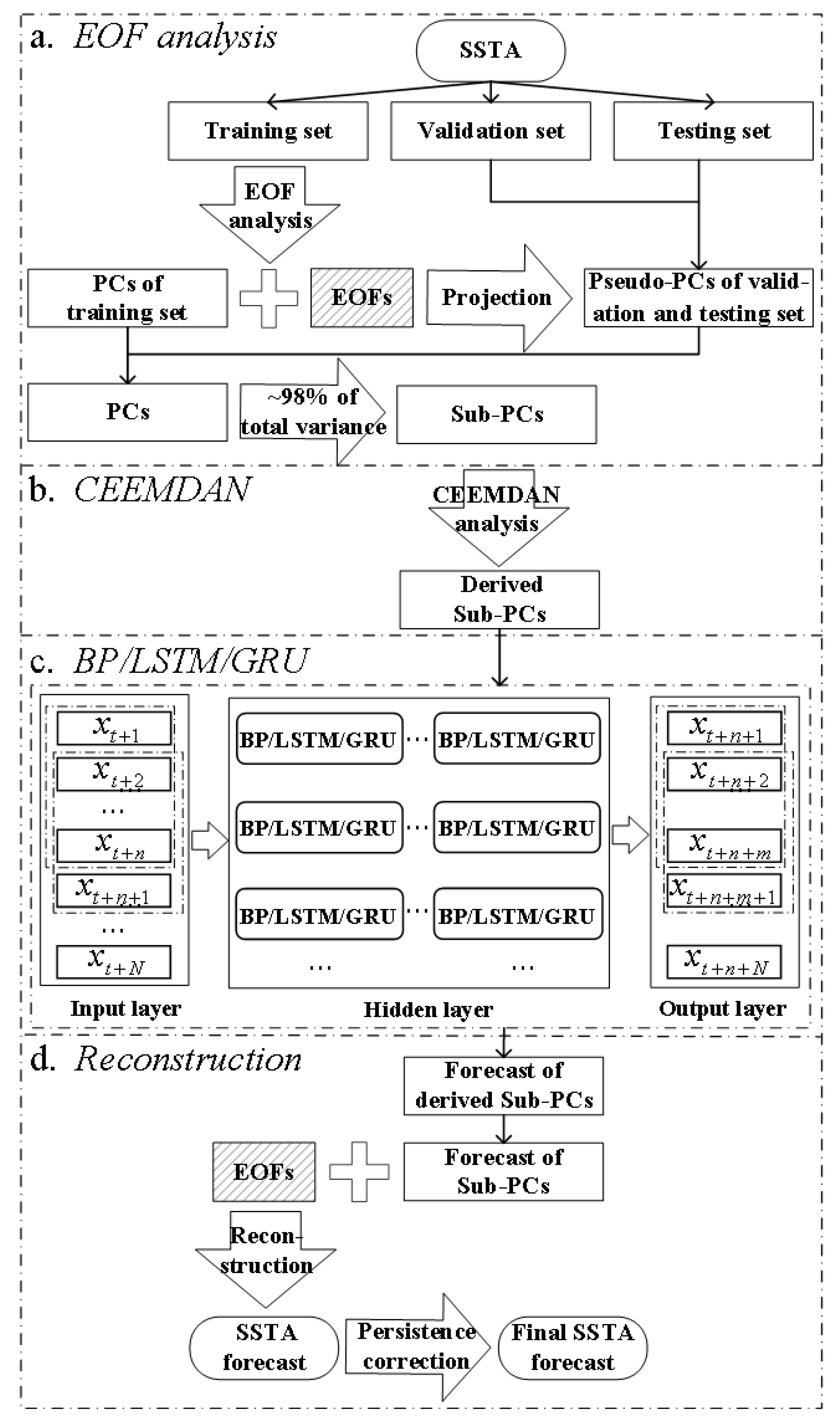
Figure 2 shows the workflow using the three deep neural networks to build the hybrid prediction models, referred to as BP, LSTM, and GRU for short, which employ BP, LSTM, and GRU deep neural networks, respectively. There are four steps in all, marked alphabetically as a, b, c, and d, to build any one of the three hybrid models as shown in Figure 2. In the first step marked with “a. EOF analysis”, the time series of the SSTA is divided into training, validation, and testing sub-datasets. The classical EOF analysis is performed on the training subset to obtain its spatial modes, called EOFs and their corresponding time series called principal components (PCs). In what follows, we find that using those spatial modes with the accumulative explained variance reaching ~98% to reconstruct the original data is enough to retain the main characteristics of the spatial structure, and by doing so, while the desired forecasting results can be reached, the computational cost of the models is reduced. Therefore, the corresponding PCs, called Sub-PCs, are used as the input series for the CEEMDAN analysis in the next step marked with “b. CEEMDAN.” Such advantage of the EOF analysis for data compression and dimensionality reduction can help accelerate computing and increase the efficiency of the proposed hybrid models. Under the assumption that the time series can be considered stationary since the length of the available training data series is reasonably long, by projecting the validation and testing subsets onto the EOFs derived from the training subset, corresponding time series called pseudo-PCs are generated and ready to be used for cross-validation to avoid overfitting and assessing the forecast skill, respectively. During the third step marked with “c. BP/LSTM/GRU”, a deep learning model, using BP, LSTM, or GRU neural network, is built to generate forecasts of the derived Sub-PCs with each of them comprised of several intrinsic mode functions and a residual from the CEEMDAN analysis. Due to the fact that these derived Sub-PCs are temporally uncorrelated, each of them can be fed into BP, LSTM, or GRU neural network separately for training; and its corresponding output can be verified with the pseudo-PCs derived from the validation and testing subsets. A complete network for BP, LSTM, or GRU is constructed in which an input, an output, and several hidden layers are involved. Each hidden layer consists of a limited number of BP, LSTM, or GRU cells. The final step, marked with “d. Reconstruction”, is the process of reconstruction, during which the predicted Sub-PCs are combined with the EOFs derived in the first step to obtain the final forecast of the SSTA field after persistence correction. Note that the ~2% leftover signals in the EOF analysis are added back to the predicted SSTA field in a manner similar to persistence at the first three days determined through weighted fitting [17] so that the full field of SSTA forecast can be achieved in this way.
The SCS SST variability is profoundly influenced by coupled atmosphere–ocean phenomena across multiple timescales, both regionally and globally. Therefore, splitting the original time series of SSTA into training, validation, and testing sub-datasets is critical to capture recurring patterns from the air–sea coupling processes within a sufficiently long training subset, which makes it possible to extend the range of skillful forecasts for the SCS SST. We divide the original time series of the 40-year satellite-based SSTA dataset into training, validation, and testing sub-datasets as follows: the first 32-year (1982−2013) data go into the training subset, the following one year (2014) data go into the validation subset for cross-validation to avoid overfitting during the training process, and the last 7-year (2015−2021) data go into the testing subset, which can be regarded as true field or observations (referred to as truth in the following text), to validate capabilities of the prediction models.
We assess the forecasts of SCS SSTA generated by the three hybrid prediction models, namely BP, LSTM, and GRU, using the statistical metrics of root mean square error (RMSE), mean error (ME, or bias), mean absolute error (MAE), spatial anomaly correlation coefficient (ACC) and time correlation coefficient as evaluation criteria. The calculation formulae are as follows:
R M S E = 1 N j = 1 N X i , j P X i , j T 2
M E = 1 N j = 1 N X i , j P X i , j T
M A E = 1 N j = 1 N X i , j P X i , j T
A C C = i = 1 M ( X i , j P X ¯ j P ) ( X i , j T X ¯ j T ) i = 1 M X i , j P X ¯ j P 2 i = 1 M X i , j T X ¯ j T 2
R = j = 1 N ( X i , j P X ¯ i P ) ( X i , j T X ¯ i T ) j = 1 N X i , j P X ¯ i P 2 j = 1 N X i , j T X ¯ i T 2
where X i , j P is the predictive SCS SSTA, and X i , j T is the verification field (truth) at the i th spatial grid point and the j th sample. ACC covers all grid points ( M = 4758 ) within the SCS basin. X ¯ j P = i = 1 M X i , j P / M and X ¯ j T = i = 1 M X i , j T / M are the basin averaged SSTA at the j th sample from the prediction and truth, respectively. X ¯ i P = j = 1 N X i , j P / N and X ¯ i T = j = 1 N X i , j T / N are the time averaged SSTA at the i th spatial grid point from the prediction and truth, respectively.
RMSE reflects the stability of the forecast model and ME can directly reflect the average deviation but may result in a situation where positive and negative values cancel out. Therefore, we also use MAE for comprehensive assessment. As a common rule of thumb used within the European Centre for Medium-Range Weather Forecasts [18], the skill in the positioning of synoptic-scale features ceases to have value for general predicting purposes where the ACC value falls below 0.6. In view of this, the forecast skill horizon in this study is defined as the lead time when the daily SSTA forecast ceases to be more skillful than the climatology [7,19] and the ACC value falls below 0.6. An ACC value of 0.6 is hereinafter referred to as the ACC threshold. We then use the results from the forecasting experiments for producing 50-day forecasts, initialized daily from 2015 to 2021, to evaluate the performances of these three hybrid models.

2.2.2. EOF Analysis

Empirical orthogonal function (EOF) analysis is a classical statistical method in the field of the atmosphere and the ocean [13]. It can quickly decompose a large amount of data and extract the main spatial structure, effectively analyzing the spatial and temporal variability of the data field while reducing dimensionality. In this study, the data matrix with the cyclic components and warming trend removed is as follows:
X = x 1,1 x 1 , n x m , 1 x m , n
where, M is the number of spatial grid points, N is the length of time series. Then, covariance matrix is constructed:
C = 1 n X × X T
The eigenvalues ( λ 1 , , λ m ) and eigenvectors V of covariance matrix are expressed as follows:
C V = V Λ
where Λ = d i a g ( λ 1 , , λ m ) , V represents the EOFs, and time coefficient or principal component PCs can be calculated:
P C = V T × X

2.2.3. CEEMDAN Method

Complete Ensemble Empirical Mode Decomposition with Adaptive Noise (CEEMDAN) is developed from EMD, EEMD, and CEEMD. These EMD-based methods can adaptively decompose original data into several Intrinsic Mode Functions (IMFs) and a residue with different frequencies and scales.
Define the operator E j ( . ) in which for the given data, it produces the j th mode obtained by EMD. Define w i ( t ) as the i th added white noise. Let x ( t ) be the original targeted data. Add white noise w i ( t ) with the original time series data so that
X i ( t ) = x ( t ) + ϵ 0 w i ( t )
where ϵ 0 is a noise coefficient. Then, decompose each x i ( t ) by the original EMD method to get the first component, i.e., first mode IMF. The first mode true IMF is the mean of all IMFs:
I M F ¯ 1 = 1 I i = 1 I I M F i 1
Next, compute the first residue component as:
R 1 ( t ) = X i ( t ) I M F 1 ¯
Then, the noise component ε 1 E 1 w i ( t ) is added to the obtained residue R 1 t ; and EMD decomposition is performed on the remaining signals after the white noise is added to obtain the second IMF component:
I M F 2 ¯ = 1 I i = 1 I   E 1 R 1 ( t ) + ε 1 E 1 w i ( t )
Repeat for other IMFs till the residue is not possible to decompose further. Final residue is computed:
R N ( t ) = X ( t ) k = 1 N   I M F k ¯
where N is the number of IMFs.
The CEEMDAN method can eliminate the modal aliasing in EMD by adding adaptive noise and can solve the non-linear and non-stationary problem by decomposing the original data into IMFs of different frequencies [20].

2.2.4. Neural Network

1. BP (Back-propagation) neural network is a multilayer feedforward neural network consisting of input, hidden, and output layers. Each layer is fully interconnected, and no interconnection exists in the same layer. One or more hidden layers can exist. The governing mathematical equations in the forward propagation mode of the BP algorithm are given as follows:
Y j = Σ i = 0 M W i j 1 X i + f 1 M
L j = f Y j
Z K = Σ j = 0 N W j K 2 L j + f 2
H = f Z K
where X i is the input vector, M is the number of input layer nodes, W is the weight value, f 1 and f 2 are the threshold parameters, Y j is the node input value of the hidden layer, L j is the output value after the nonlinear transfer function, f is activation function, N is the number of hidden layer nodes, Z k is the input value of the output layer node and H is the output value of the output layer node. If the output results do not match the expectations, then they enter the reverse propagation process. The governing mathematical equations of reverse propagation process are given as follows:
W j i t = W j i t 1 + η a ρ j t x i t + α a Δ W j i t
f j t = f j t + η b ρ j t x i t + α b Δ f j t
ρ t = 1 2 p = 1 G H H ^ 2
α is the momentum constant, η refers to the learning rates, ρ is error signal, G is the number of data in the training data set, H and H ^ is the desired output and actual output, respectively. The process of forward and backward propagations is repeated until the error between the output and the expectation is reduced to an acceptable level or the number of learning times reaches a predetermined value [21].
2. Long Short-Term Memory (LSTM) neural network is a variation of the recursive neural network (RNN), which is mainly used to solve the problems of gradient disappearance and gradient explosion in the process of long-sequence training [22]. LSTM have gating mechanisms in each cell where three different input types are fed into, these are x t , h t 1 , and C t 1 . The governing mathematical equations in LSTM networks are given as follows:
f t = σ W f h t 1 , x t + b f
i t = σ W i h t 1 , x t + b i
o t = σ W o h t 1 , x t + b o
C ~ t = tan h W c h t 1 , x t + b c
C t = f t × C t 1 + i t × C ~ t
h t = o t × tan h C t
where h t and C t are hidden layer vectors, x t is input vector, b f , b i , b C and b o are bias vectors, W f , W i , W C and W o are parameter matrices, and σ and t a n h are activation functions [23].
3. Gated Recurrent Unit (GRU) neural networks possess a similar cell structure to LSTM networks. However, their simpler gating mechanisms in comparison with LSTM networks allow the system to perform complex computations with fewer resources in a lesser amount of time. Thus, the training of these networks is performed at a higher speed [24]. One of the main differences between GRU and LSTM networks is the fact that, unlike LSTM networks, GRU networks combine the cell state and hidden state in one variable, namely ht. The mathematical operations which allow GRU networks to accomplish the above operations are given as follows:
z t = σ W z h t 1 , x t + b z
r t = σ W τ h t 1 , x t + b τ
h t = tan h W h r t     h t 1 , x t + b h
h t = 1 z t     h t 1 + z t     h t
where h t are hidden layer vectors, x t are input vectors, b z , b r , and b h are bias vectors, W z , W r , and W h are parameter matrices [24].
The critical parameters adopted in these three hybrid models were determined through tuning experiments by achieving the best performance of the model. In the end, we build unified three-layer neural networks and each layer has 100 neurons. The input length is set to 30 and the output length is set to 50 by trial and error, which means that we use the previous 30 days of the data for predicting the next 50 days. In addition, we use adaptive moment estimation (Adam) as the gradient optimization algorithm, which has the advantages of high computational efficiency and better learning effect. The rectified linear unit (ReLU) function is used as the activation function, which avoids the gradient vanishing problem of sigmoid function and tanh function. The batch size for training is set to 500.

3. Results

3.1. Forecasts Verification

To assess the overall performances of these three hybrid models, we calculated the averaged MAE, RMSE and ACC as a function of the forecast horizon length over the period 2015–2021 (Figure 3). The corresponding MAE, RMSE and ACC of the persistence (dark blue bars), a reference forecast obtained by persisting the initial SSTA field across all lead times, are also presented in Figure 3 to provide a baseline for evaluating the model forecasts. While the SCS SSTA has a persistence length of 18 (22) days as indicated by the RMSE (MAE) of persistence crossing climatology ~0.75 °C (~0.61 °C), the ACC of persistence forecast falls below 0.6 on day 5. This illustrates that, by comparison, ACC is a stricter criterion than MAE and RMSE for measuring the forecast skill horizon. As such, the above-mentioned 50-day forecast horizon used in the SSTA forecasting experiments is actually defined according to the ACC threshold of 0.6. Results indicate that, on average, all three models are equally capable of providing skillful forecasts of the daily SCS SSTAs out to 50 days in terms of MAE, RMSE and ACC. The forecast skill scores for the three models are overall notably higher than persistence or climatology forecasts at all lead times. For each of them, RMSE (MAE) rises steadily as lead time increases. An averaged RMSE (MAE) of ~0.48 °C (~0.37 °C) is attained at the end of the 50-day forecast window, which is up to 36% (39%) smaller than climatology. ACC declines more quickly than the rise in MAE and RMSE, especially when the forecast lead time is shorter than ~15 days. An averaged ACC of ~0.63 is attained at the end of the 50-day forecast window, which is up to four times larger than persistence. This indicates that, on average, the forecast skill horizon for all three models is beyond the available forecast length (50 days) in terms of MAE, RMSE and ACC.
Given their capabilities of learning time sequences by exhibiting almost the same forecast performance, whereas the BP model actually executed faster and only took around 20% of the running time of either LSTM or GRU model for implementing 50-day forecasting experiments over the period 2015–2021, in what follows, only those results from the BP model are examined in detail.
Figure 4 shows the boxplots of the bias as a function of forecast lead time for the daily SCS SSTA forecasts. The dot in each box denotes the mean value, while box limits indicate the range of the central 50% of the bias, with the central line within the box marking the median and the circles above and below the whiskers representing the outliers that are either above 99.5th or below 0.5th percentile. As expected, the spread of the bias shows a tendency for increasing with increasing lead; and such increasing tendency becomes slow at lead times longer than ~15 days in terms of both interquartile range (box) and whiskers (dashed lines). The 99% forecast bias remains within the range of approximately −0.57 °C to 0.59 °C at the end of the 50-day forecast window. The daily SCS SSTA forecasts are warm biased, according to the medians (or means), just a little bit, with relatively large values (less than 0.04 °C in terms of median or mean) observed in the middle of the forecast range, i.e., at lead times of 20–35 days. It is clear that more warm outliers than cold ones exist at the lead times longer than one day.
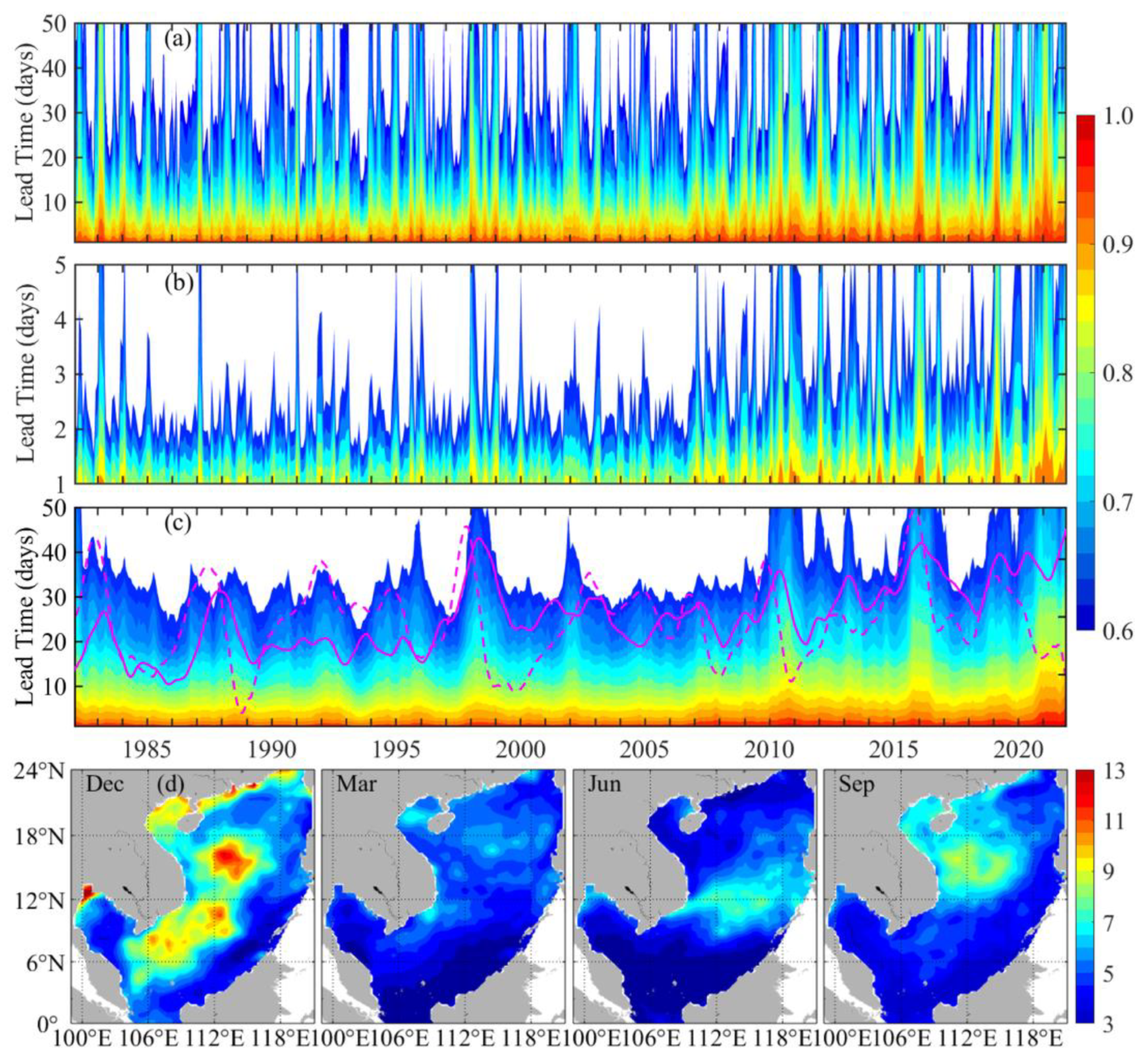
We are also interested in the forecast skill horizon for the instantaneous SSTA forecast generated by the BP model on individual days. The basin averaged daily RMSE and ACC for the SCS SSTA forecast are presented in Figure 5a,c as a function of forecast lead time from one to 50 days for the period 2015–2021. For comparison, the persistence forecast results are shown in Figure 5b,d. When the RMSE (ACC) for each individual day is larger (smaller) than the climatology (ACC threshold), a blank area is shown. As the blank areas in the RMSE of the BP model’s forecasts (Figure 5a) are difficult to see, black arrows are used to indicate them at the top of the panel. More blank areas are in Figure 5c,d for ACC than in Figure 5a,b for RMSE for both the model and persistence, because, as indicated above, ACC is a stricter skill metric than RMSE. In fact, Figure 5a (Figure 5c) shows that there are ~3% (~41%) of the total forecast days when the RMSE (ACC) of the BP model is less skillful relative to the climatology (the ACC threshold) to provide SSTA forecasts out to the 50 days during the period 2015–2021; for persistence, Figure 5b (Figure 5d) shows the initial SSTA field can be persisted across the 50 days for 5% of the total forecast days (only a few days during the first half of 2019) in terms of RMSE (ACC). The least forecast skill horizons of the daily SCS forecasts for the BP model and persistence determined by RMSE (ACC) are 14 and 2 days (5 and 1 day(s)), respectively.
Note that the forecast skill lengths of the BP model have been simultaneously extended over persistence in terms of both RMSE and ACC. The BP model has skill clearly out to 50 days in the forecasts with remarkably high ACCs when the SCS SSTAs have the most significant persistence; for example, those time bands starting roughly from the beginning of 2016, 2019, and 2021, respectively, as shown in Figure 5d.
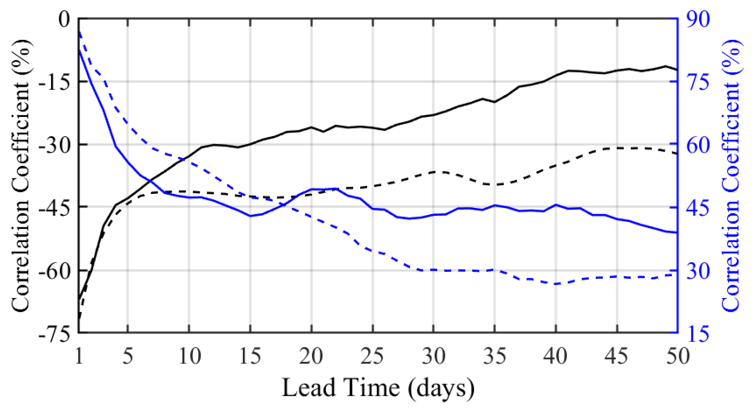
The daily RMSE and ACC time series of the BP model (blue solid and dashed lines in Figure 6) are correlated well with those of persistence at the beginning of the 50-day forecast window, especially the ACC (blue dashed line in Figure 6). The correlation coefficient for RMSE (ACC) at forecast lead time of one day is as high as ~82% (~87%), it then declines rapidly at lead times up to ~15 (30) days with ~43% (~30%) being attained, and then maintains relatively large (small) fluctuations till the end of the forecast window.
The smaller (larger) the RMSE (ACC), the better the model fits the truth. As shown in Figure 5, for forecast lead times less than a few days, small daily RMSEs always correspond to large ACCs for the BP model and persistence forecasts, and vice versa. This can be further identified by the fact that, at a forecast lead time of one day, the correlation coefficient between RMSE and ACC time series from the BP model (persistence) is ~67% (~72%), as indicated by the black solid (dashed) line in Figure 6; it then goes down quickly with increasing lead for the first few days, especially for the BP model forecasts. At a forecast lead time of five days, for example, it drops to ~43% (~44%) for the model (persistence) forecasts. After that, the correlation between the RMSE and ACC time series produced by the persistence remains almost unchanged (~42%) at forecast lead times shorter than ~20 days and then decreases with forecast lead time at a relatively slow rate and reaches ~32% at the end of the forecast window. For the model forecasts, the correlation between the RMSE and ACC time series slowly reduces to approximately 13% at a forecast lead time of ~41 days, and then stays almost unchanged till the end of the forecast window.
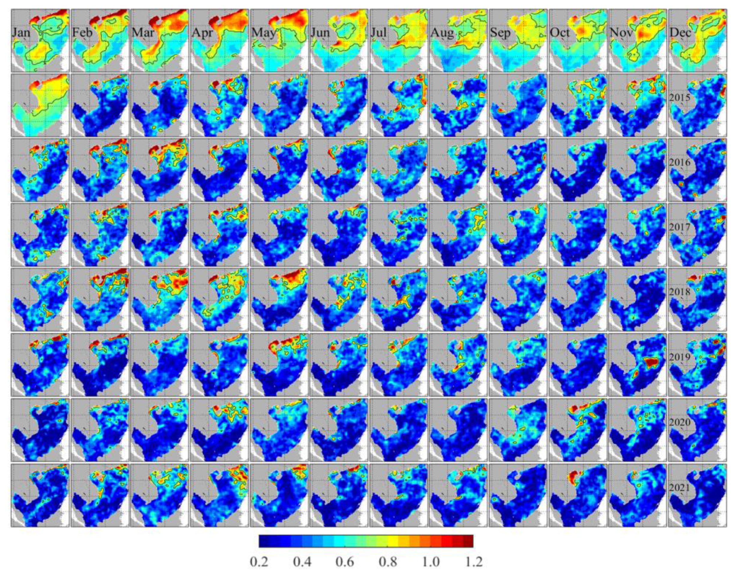
To evaluate the spatial distribution of the model forecast skill, we calculate the monthly mean RMSEs in the model forecasts for each grid at lead times of 1–50 days first for the period 2015–2021. Only those at lead time of 50 days are plotted in Figure 7 (second row onward, excluding the first panel in the second row that is the annual SSTA climatology), which means these maps are valid at the 50-day forecast time. Monthly SSTA climatology is shown in the first row. Since the forecasting experiment started on 1 January 2015, the monthly mean RMSE at lead time of 50 days is not available for the month of January; and only forecasts for the last 10 days were used to calculate monthly mean RMSE for the month of February in year 2015.
As shown in the first panel of the second row of Figure 7, the isotherms of the annual SSTA climatology are oriented along an axis in the northeast-to-southwest direction. Spatial variability of the annual mean SSTA in the northern SCS region is larger than the mean value (~0.75 °C) in the entire basin as shown by black contours, and smaller than that in the south. The same situation applies for most months, as indicated in the top panels of Figure 7. The large variability of the SSTA in the north is actually a potential barrier to the learning ability of the model in a long-range forecast, which can be confirmed from the similar spatial distribution of the monthly mean RMSEs of the model forecasts at a lead time of 50 days, as seen in the panels from the second to last row in Figure 7. At first glance, the monthly mean RMSEs of the model forecasts at the end of the 50-day window for the period 2015–2021 are apparently smaller than the corresponding monthly climatologies in most regions and months; and the predictability for the southern region is clearly higher than that for the northern region. The months with relatively large errors in the northern region include early spring months in 2016 (see the third panel in the third row of Figure 7), and late-winter and spring months in 2018 (see the second to fifth panels in the fifth row of Figure 7). This also happens to correspond to relatively large variability of the monthly mean SSTA in the meantime in the northern SCS (from February to May in the top panels of Figure 7). November 2019 is an exception with large errors occurring in the deep-water area of the central SCS (see the next to last panel in the sixth row of Figure 7).
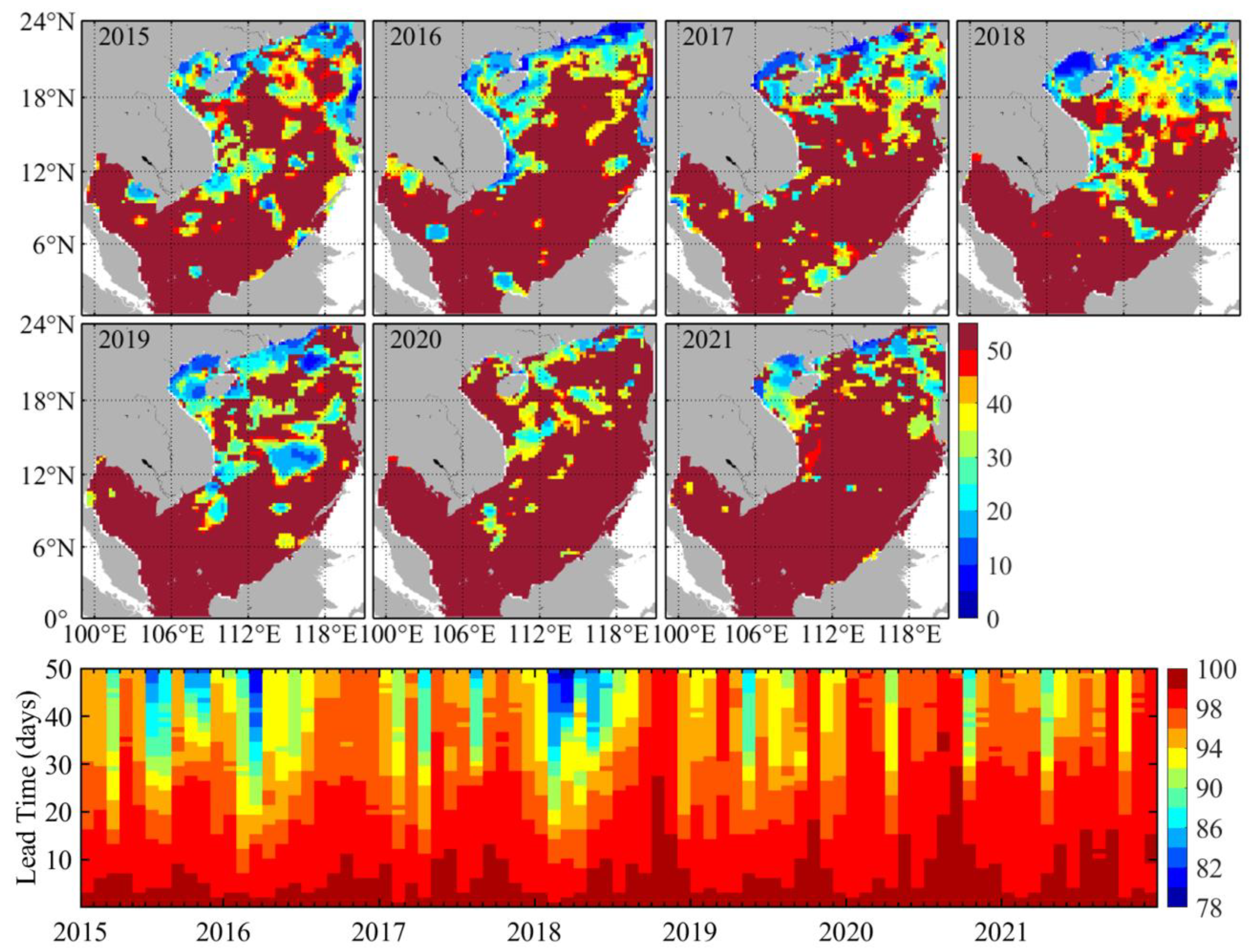
Next, the forecast skill horizon on which the RMSE crosses the monthly mean climatology is identified for each grid and each month. Then, the composite map of the forecast skill horizon for the entire SCS basin for each year from 2015 to 2021 is obtained by keeping the least forecast skill horizon for each grid among 12 months in that year and plotted in the top and middle panels of Figure 8. Meanwhile, the numbers of grids with the monthly mean RMSE of the model forecasts smaller than the corresponding monthly mean climatology are derived at lead times of 1–50 days for the period 2015–2021. The frequencies characterizing the proportion of these grid numbers of the entire SCS basin for each month during the period 2015–2021 are shown in the bottom panel of Figure 8.
The model performs better than monthly climatology out to 50 days in most regions of the southern SCS basin, in particular in year 2021, based on the composite map of the forecast skill horizon measured by RMSE for each year during the period 2015–2021 (top and middle panels in Figure 8). Lower predictability is observed in the northern region, especially along the coastal regions and within the Beibu Gulf in most years, which is consistent with the spatial distribution of the monthly SSTA climatology. The least forecast skill horizon is only one day determined by the monthly climatology (see dark blue in the top and middle panels of Figure 8). The bottom panel of Figure 8 shows that for the entire SCS basin there are actually at least ~78% grids in each month when the RMSE is smaller than the corresponding monthly climatology during the period 2015–2021. The number of grids occupies a relatively small proportion in March 2016 and late-winter and spring months of 2018 for the lead times is longer than 30 days, which is consistent with the time periods during which relatively large monthly mean RMSEs in the model forecasts occur.

3.2. Time Scales of Forecast Skill Horizon

The forecast skill horizon in terms of ACC for the daily SCS forecast of the model exhibits prominent features with multiple time scales (Figure 5c). In light of this, we focus more on the ACC next. To find dominant temporal modes of variability associated with the forecast skill horizon, we obtain the wavelet power spectrum [25] for the time series of the forecast skill horizon determined by the ACC threshold of 0.6 for each individual daily SCS forecast during the period 1982–2021 (Figure 9, left panel). Here, we employ the complete SSTA time series, not just the testing sub-dataset, so that longer time-scale features embedded in the forecast skill horizon can be extracted. Global wavelet spectrum (Figure 9, right panel) is calculated by averaging the wavelet power spectrum over time. The most distinct peak revealed in the computed global wavelet spectrum is a sharp maximum at a period of about one year, which persists throughout almost the entire time period. Other significant peaks exceeding the 95% confidence level for a red-noise process in the computed spectrum are observed at about 60 days, six months, in the range of 2–5 years, and ≥~10 years. The wavelet power spectrum (Figure 9, left panel) is clearly nonstationary in these period bands. Next, we perform preliminary explorations to try to relate these significant wavelet peaks to various regional and global coupled air–sea phenomena.
The strong annual maximum revealed in the computed global wavelet spectrum is associated with the fact that the forecast skill horizon tends to be longer and out to 50 days in most cases during the winter months for the period 1982–2021 as illustrated by the monthly mean ACCs of the daily SCS SSTA forecasts produced by the model (Figure 10a). As has been demonstrated in Figure 6, a good correlation (>66%) is found between the daily ACCs in the forecasts of the BP model and persistence (blue dashed line) at lead times shorter than ~5 days. And this conclusion still holds for the monthly ACCs by comparing Figure 10a,b, in which the monthly ACCs for persistence at lead times of 1–5 days are displayed. Such annual phasing of inter-annual SSTA strong persistence is consistent with the fact that the temporal persistence of the SCS SSTAs is seasonally varying, which is the greatest in winter (Figure 10d). It may be due to, as explained in [26], that the winter SSTAs that persisted at depth below the shallow mixed layer during the summer months become re-entrained into the mixed layer during the following winter.
The band of peaks between about 2 and 5 years in the computed spectrum is thought to be related to the prominent interannual signal of the ENSO events. As noted, interannual variability of the SCS SSTA is significantly correlated with the ENSO signals [8]. To look into this, we obtain the smoothed ACCs (Figure 10c), with a 12-month running mean filter applied to the monthly mean ACCs in Figure 10a, at lead times of 1–50 days for the period 2015–2021. Whilst the highest correlation coefficient of ~0.46 between the basin monthly SCS SSTA (purple solid line in Figure 10c) and Niño 3.4 index (purple dashed line in Figure 10c) is found when the former lags the latter by five months, the interannual variation of the forecast skill horizon is correlated well with the basin averaged monthly SCS SSTA (Figure 10c). During the warm episodes of the ENSO (El Niño), higher predictability is evident with the forecast skill horizon easily extending out to 50 days associated with the El Niño events in 1997–1999, 2009–2010, and 2015–2016.
The semi-annual cycle in the computed spectrum corresponding to relatively strong persistence in the monthly ACCs (Figure 10b) may be mainly affected by monsoons over the SCS [28,29]. The first peak near 60 days in the computed spectrum may correspond to an intraseasonal cycle, which is the coupled result of intraseasonal SST variation with atmospheric intraseasonal oscillations [30]. The last significant peak around 10 years in the spectrum, just exceeding the 95% confidence level, perhaps matches the decadal change in the intraseasonal variability of SSTA [31] or is induced by the PDO [8]. All of these preliminary inferences need to be verified through further exploration in the future.
The persistence of the SCS SSTA became stronger after 2007 (Figure 10b), with the most significant persistence occurring in the early spring months of 2019 (see Figure 5d). At the same time, the model performance is accordingly enhanced on the basis of persistence after 2007; and the forecast skill horizon of the model can be extended out to 50 days more easily and frequently with relatively high ACCs (Figure 10c). This is another interesting topic worthy of in-depth investigation in the future.

3.3. Impact of Tropical Cyclones

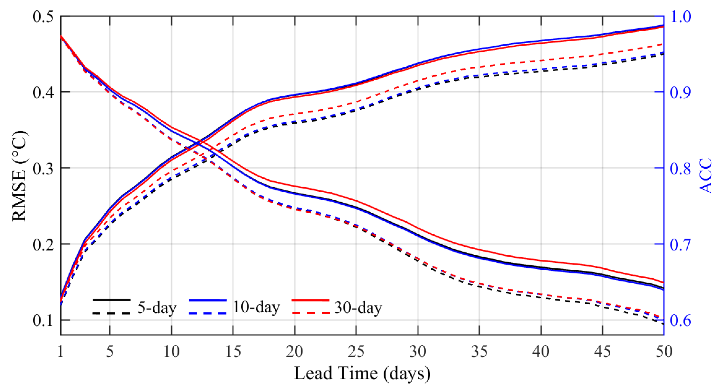
To demonstrate the impact of severe weather systems, such as tropical cyclones (TCs), on the performance of the model forecast, we examine the forecast results under normal and severe weather conditions separately. The TC track data used are from the China Meteorological Administration (CMA) best track dataset [32]. There were a total of 65 TCs from 2015 to 2021. Following [17,33,34], we use 5 days (Figure 11, black lines), 10 days (Figure 11, blue lines) and 30 days (Figure 11, red lines) before and after the TC passage plus the duration of the TC as the time window of severe weather condition. As shown in Figure 11, the ACC under normal weather conditions is higher than that under severe weather conditions as the forecast length increases; and yet the averaged ACC at the end of the 50-day forecast cycle under a 10-day and 30-day time window of severe weather conditions is still higher than the threshold of 0.6. On the contrary, the RMSE under normal weather conditions is larger than that under severe weather conditions as forecast length increases (the solid blue line and the solid black line overlap). Notice that Shao et.al obtained the same results [17], which will be an interesting topic for future discussions.
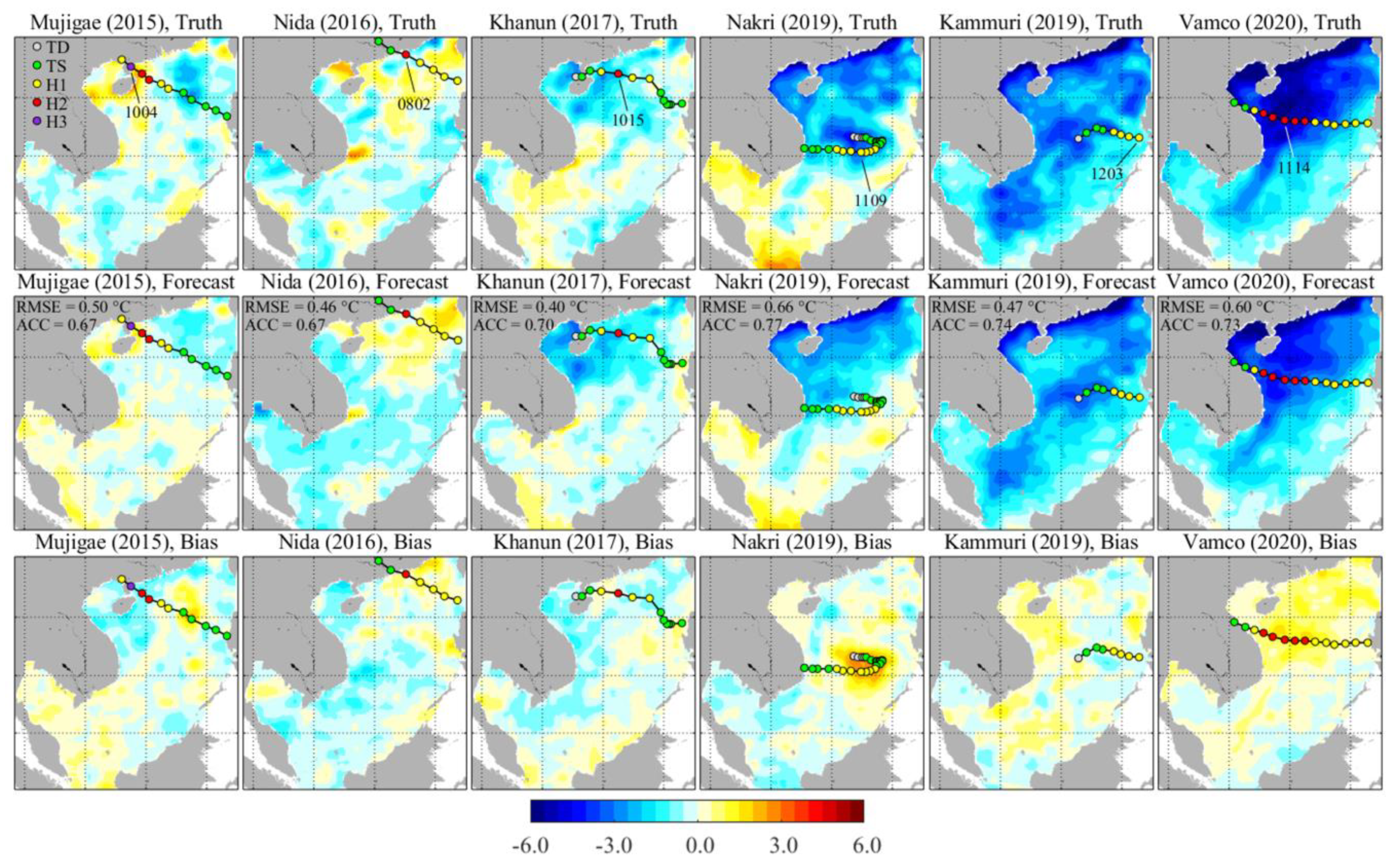
Six out of the 65 TCs passing over the SCS were classified as typhoons. They are used to examine the performance of the model when the forecast skill horizon is out to 50 days. For each of these six typhoon cases, the SST changes on the day when the typhoon reaches its peak intensity and is calculated over the 50-day forecast window for the truth and forecast. As shown in the bottom panels of Figure 12, the bias in the SSTA forecast is not evident during the passage of the typhoon except for Nakri (2019), with both the RMSE (0.66 °C) and ACC (0.79) of the SCS SSTA forecasts being the maximum among the six typhoon cases.
Such performance achieved by the model under a severe weather system indicates that, due primarily to its short life span and limited impact area, TC is not necessarily an obstacle to the predictability of SCS SSTA in the long range.

4. Discussion

The overall performances show that the hybrid deep learning-based prediction models established in this study, namely BP, LSTM, and GRU, demonstrate equal capabilities and can skillfully extend the daily SCS SSTA forecasting lead time to 50 days in terms of both RMSE and ACC. This is comparable to the state-of-the-art operational systems in long-range forecasting, such as the Navy-ESPC. It shows that the forecast skill horizon for each individual day measured by ACC, ranging from 5 to 50 days, exhibits prominent features with multiple time scales. The significant periods revealed by the computed spectra of the forecast skill horizon time series corresponding to the ACC threshold of 0.6 include those of ~60 days, six months, one year, in the range of 2–5 years, and about ≥10 years. Preliminary explorations demonstrate that such evident variability on time scales from intraseasonal to decadal embedded in SCS SST fluctuations in nature caused by various mechanisms, including internal ocean variability, local and remote stochastic atmospheric heat and momentum flux forcing, can be extracted by the proposed hybrid algorithms to realize long lead-time forecasting. In addition, data-driven mechanisms represent a valuable opportunity to unmask the physics that we do not yet know [35].
Challenges remain for deep learning-based algorithms to implement daily SSTA forecasting skillfully at long lead times for each individual day. Reliable time series data are not as abundant and long enough right now, which hinders the long-range prediction ability of data-driven models and their wide range applications, such as forecasting subsurface ocean variables. One way for achieving skillful forecasts at long lead times consistently is to develop a class of models that are driven by data and obey physical principles and then combine their advantages. Yet, to increase the prediction length, identifying the factors that impact the SSTA evolution in the coupled atmosphere–ocean system involved different atmospheric and oceanic processes with highly complicated variability in both space and time has always been the central focus and the challenge for the development of physics-based models.

Author Contributions

Conceptualization, G.H., Q.S. and W.L.; methodology, M.Z., G.H., X.W. (Xiaobo Wu), C.L., Q.S., W.L. and X.W. (Xuan Wang); software, M.Z., X.W. (Xiaobo Wu) and L.C.; validation, M.Z., G.H., X.W. (Xiaobo Wu), L.C., W.D. and Z.J.; formal analysis, M.Z., G.H., Q.S., W.L. and X.W. (Xuan Wang); investigation, M.Z., G.H., X.W. (Xiaobo Wu), L.C., W.D. and Z.J.; resources, G.H., W.L. and X.W. (Xuan Wang); data curation, M.Z., C.L. and L.C.; writing—original draft preparation, M.Z., G.H. and C.L.; writing—review and editing, M.Z., G.H. and X.W. (Xiaobo Wu); visualization, M.Z.; supervision, G.H.; project administration, G.H.; funding acquisition, G.H. and W.L. All authors have read and agreed to the published version of the manuscript.

Funding

This research was supported in part by the National Key Research and Development Program under Grant 2023YFC3107800 and in part by the National Natural Science Foundation under Grants 42376190 and 41876014.

Data Availability Statement

All data used are publicly available and their sources are stated in the acknowledgments.

Acknowledgments

The authors thank the following data and tool providers: NOAA for OISST-V2.1-AVHRR data, available at https://www.ncdc.noaa.gov/oisst (accessed on 9 March 2024) and Niño3.4 index, available at https://psl.noaa.gov/data/timeseries/monthly/NINO34/ (accessed on 9 March 2024), CMA for typhoon data, available at https://tcdata.typhoon.org.cn/ (accessed on 9 March 2024), Google for machine learning-related open-source software including TensorFlow, available at https://www.tensorflow.org/ (accessed on 9 March 2024), Keras, available at https://keras.io/ (accessed on 9 March 2024), and Scikit-learn, available at http://scikit-learn.org/stable/ (accessed on 9 March 2024).

Conflicts of Interest

The authors declare no conflicts of interest.

References

  1. Reichstein, M.; Camps-Valls, G.; Stevens, B.; Jung, M.; Denzler, J.; Carvalhais, N.; Prabhat. Deep learning and process understanding for data-driven Earth system science. Nature 2019, 566, 195–204. [Google Scholar] [CrossRef]
  2. Zheng, G.; Li, X.; Zhang, R.-H.; Liu, B. Purely satellite data-driven deep learning forecast of complicated tropical instability waves. Sci. Adv. 2020, 6, eaba1482. [Google Scholar] [CrossRef]
  3. Aparna, S.G.; D’souza, S.; Arjun, N.B. Prediction of daily sea surface temperature using artificial neural networks. Int. J. Remote Sens. 2018, 39, 4214–4231. [Google Scholar] [CrossRef]
  4. Xiao, C.; Chen, N.; Hu, C.; Wang, K.; Gong, J.; Chen, Z. Short and mid-term sea surface temperature prediction using time-series satellite data and LSTM-AdaBoost combination approach. Remote Sens. Environ. 2019, 233, 111358. [Google Scholar] [CrossRef]
  5. Shao, Q.; Hou, G.; Li, W.; Han, G.; Liang, K.; Bai, Y. Ocean reanalysis data-driven deep learning forecast for sea surface multivariate in the South China Sea. Earth Space Sci. 2021, 8, e2020EA001558. [Google Scholar] [CrossRef]
  6. Shao, Q.; Li, W.; Hou, G.; Han, G.; Wu, X. Mid-term simultaneous spatiotemporal prediction of sea surface height anomaly and sea surface temperature using satellite data in the South China Sea. IEEE Geosci. Remote Sens. Lett. 2022, 19, 1–5. [Google Scholar] [CrossRef]
  7. Barton, N.; Metzger, E.J.; Reynolds, C.A.; Ruston, B.; Rowley, C.; Smedstad, O.M.; Ridout, J.A.; Wallcraft, A.; Frolov, S.; Hogan, P.; et al. The Navy’s Earth System Prediction Capability: A new global coupled atmosphere-ocean-sea ice prediction system designed for daily to subseasonal forecasting. Earth Space Sci. 2021, 8, e2020EA001199. [Google Scholar] [CrossRef]
  8. Thompson, B.; Tkalich, P.; Malanotte-Rizzoli, P. Regime shift of the South China Sea SST in the Late 1990s. Clim. Dyn. 2017, 48, 1873–1882. [Google Scholar] [CrossRef]
  9. Reynolds, R.W.; Smith, T.M.; Liu, C.; Chelton, D.B.; Casey, K.S.; Schlax, M.G. Daily high-resolution-blended analyses for sea surface temperature. J. Clim. 2007, 20, 5473–5496. [Google Scholar] [CrossRef]
  10. Thomson, R.E.; Emery, W.J. Chapter 4-The spatial analyses of data fields. In Data Analysis Methods in Physical Oceanography, 3rd. ed.; Thomson, R.E., Emery, W.J., Eds.; Elsevier: Boston, MA, USA, 2014; pp. 313–424. [Google Scholar] [CrossRef]
  11. Fang, G.; Chen, H.; Wei, Z.; Wang, Y.; Wang, X.; Li, C. Trends and interannual variability of the South China Sea Surface winds, surface height, and surface temperature in the recent decade. J. Geophys. Res. Ocean. 2006, 111, C11. [Google Scholar] [CrossRef]
  12. Yu, Y.; Zhang, H.-R.; Jin, J.; Wang, Y. Trends of sea surface temperature and sea surface temperature fronts in the South China Sea during 2003–2017. Acta Oceanol. Sin. 2019, 38, 106–115. [Google Scholar] [CrossRef]
  13. Lorenz, N.E. Empirical orthogonal functions and statistical weather prediction. In Statistical Forecasting Project Report; Department of Meteorology; Massachusetts Institute of Technology: Cambridge, MA, USA, 1956; Volume 1, pp. 1–49. [Google Scholar] [CrossRef]
  14. Torres, M.E.; Colominas, M.A.; Schlotthauer, G.; Flandrin, P. A Complete Ensemble Empirical Mode Decomposition with Adaptive Noise. In Proceedings of the 2011 IEEE International Conference on Acoustics, Speech and Signal Processing (ICASSP), Prague, Czech Republic, 22–27 May 2011; pp. 4144–4147. [Google Scholar] [CrossRef]
  15. Pai, S.; Sun, Z.; Hughes, T.W.; Park, T.; Bartlett, B.; Williamson, I.A.D.; Minkov, M.; Milanizadeh, M.; Abebe, N.; Morichetti, F.; et al. Experimentally realized in situ backpropagation for deep learning in photonic neural networks. Science 2023, 380, 398–404. [Google Scholar] [CrossRef]
  16. Kartal, S. Assessment of the spatiotemporal prediction capabilities of machine learning algorithms on sea surface temperature data: A comprehensive study. Eng. Appl. Artif. Intell. 2023, 118, 105675. [Google Scholar] [CrossRef]
  17. Shao, Q.; Li, W.; Han, G.; Hou, G.; Liu, S.; Gong, Y.; Qu, P. A deep learning model for forecasting sea surface height anomalies and temperatures in the South China Sea. J. Geophys. Res. Ocean. 2021, 126, e2021JC017515. [Google Scholar] [CrossRef]
  18. Pendlebury, S.F.; Adams, N.D.; Hart, T.L.; Turner, J. Numerical weather prediction model performance over high southern latitudes. Mon. Weather. Rev. 2003, 131, 335–353. [Google Scholar] [CrossRef]
  19. Thoppil, P.G.; Frolov, S.; Rowley, C.D.; Reynolds, C.A.; Jacobs, G.A.; Joseph Metzger, E.; Hogan, P.J.; Barton, N.; Wallcraft, A.J.; Smedstad, O.M.; et al. Ensemble forecasting greatly expands the prediction horizon for ocean mesoscale variability. Commun. Earth Environ. 2021, 2, 89. [Google Scholar] [CrossRef]
  20. Zhou, F.; Huang, Z.; Zhang, C. Carbon Price Forecasting Based on CEEMDAN and LSTM. Appl. Energy 2022, 311, 118601. [Google Scholar] [CrossRef]
  21. Liu, Y.; Zhao, Q.; Yao, W.; Ma, X.; Yao, Y.; Liu, L. Short-Term Rainfall Forecast Model Based on the Improved BP–NN Algorithm. Sci. Rep. 2019, 9, 19751. [Google Scholar] [CrossRef]
  22. Hochreiter, S.; Schmidhuber, J. Long Short-Term Memory. Neural Comput. 1997, 9, 1735–1780. [Google Scholar] [CrossRef]
  23. Zor, K.; Buluş, K. A Benchmark of GRU and LSTM Networks for Short-Term Electric Load Forecasting. In Proceedings of the 2021 International Conference on Innovation and Intelligence for Informatics, Computing, and Technologies (3ICT), Online, 29–30 September 2021; pp. 598–602. [Google Scholar]
  24. Ozdemir, A.C.; Buluş, K.; Zor, K. Medium- to Long-Term Nickel Price Forecasting Using LSTM and GRU Networks. Resour. Policy 2022, 78, 102906. [Google Scholar] [CrossRef]
  25. Torrence, C.; Compo, G.P. A practical guide to wavelet analysis. Bull. Am. Meteorol. Soc. 1998, 79, 61–78. [Google Scholar] [CrossRef]
  26. Bulgin, C.E.; Merchant, C.J.; Ferreira, D. Tendencies, variability and persistence of sea surface temperature anomalies. Sci. Rep. 2020, 10, 7986. [Google Scholar] [CrossRef] [PubMed]
  27. Ding, R.; Li, J. Decadal and seasonal dependence of North Pacific sea surface temperature persistence. J. Geophys. Res. (Atmos.) 2009, 114, D01105. [Google Scholar] [CrossRef]
  28. Du, Y.; Wang, D.; Xie, Q. Harmonic analysis of sea surface temperature and wind stress in the vicinity of the maritime continent. J. Meteorol. Res. 2003, 17, 226–237. Available online: http://jmr.cmsjournal.net/article/id/1549 (accessed on 9 March 2024).
  29. Yan, Y.; Wang, G.; Chen, C.; Ling, Z. Annual and semiannual cycles of diurnal warming of sea surface temperature in the South China Sea. J. Geophys. Res. Ocean. 2018, 123, 5797–5807. [Google Scholar] [CrossRef]
  30. Wu, R.; Cao, X.; Chen, S. Covariations of SST and surface heat flux on 10–20 day and 30–60 day time scales over the South China Sea and western North Pacific. J. Geophys. Res. Atmos. 2015, 120, 12486–12499. [Google Scholar] [CrossRef]
  31. Kajikawa, Y.; Yasunari, T.; Wang, B. Decadal change in intraseasonal variability over the South China Sea. Geophys. Res. Lett. 2009, 36, GL037174. [Google Scholar] [CrossRef]
  32. Lu, X.; Yu, H.; Ying, M.; Zhao, B.; Zhang, S.; Lin, L.; Bai, L.; Wan, R. Western North Pacific tropical cyclone database created by the China Meteorological Administration. Adv. Atmos. Sci. 2021, 38, 690–699. [Google Scholar] [CrossRef]
  33. Dare, R.A.; McBride, J.L. Sea surface temperature response to tropical cyclones. Mon. Weather. Rev. 2011, 139, 3798–3808. [Google Scholar] [CrossRef]
  34. Mei, W.; Lien, C.-C.; Lin, I.-I.; Xie, S.-P. Tropical cyclone–induced ocean response: A comparative study of the South China Sea and tropical Northwest Pacific. J. Clim. 2015, 28, 5952–5968. [Google Scholar] [CrossRef]
  35. Klie, H. A Tale of Two Approaches: Physics-Based vs. Data-Driven Models. The Way Ahead. 2021. Available online: https://jpt.spe.org/twa/a-tale-of-two-approaches-physics-based-vs-data-driven-models (accessed on 9 March 2024).
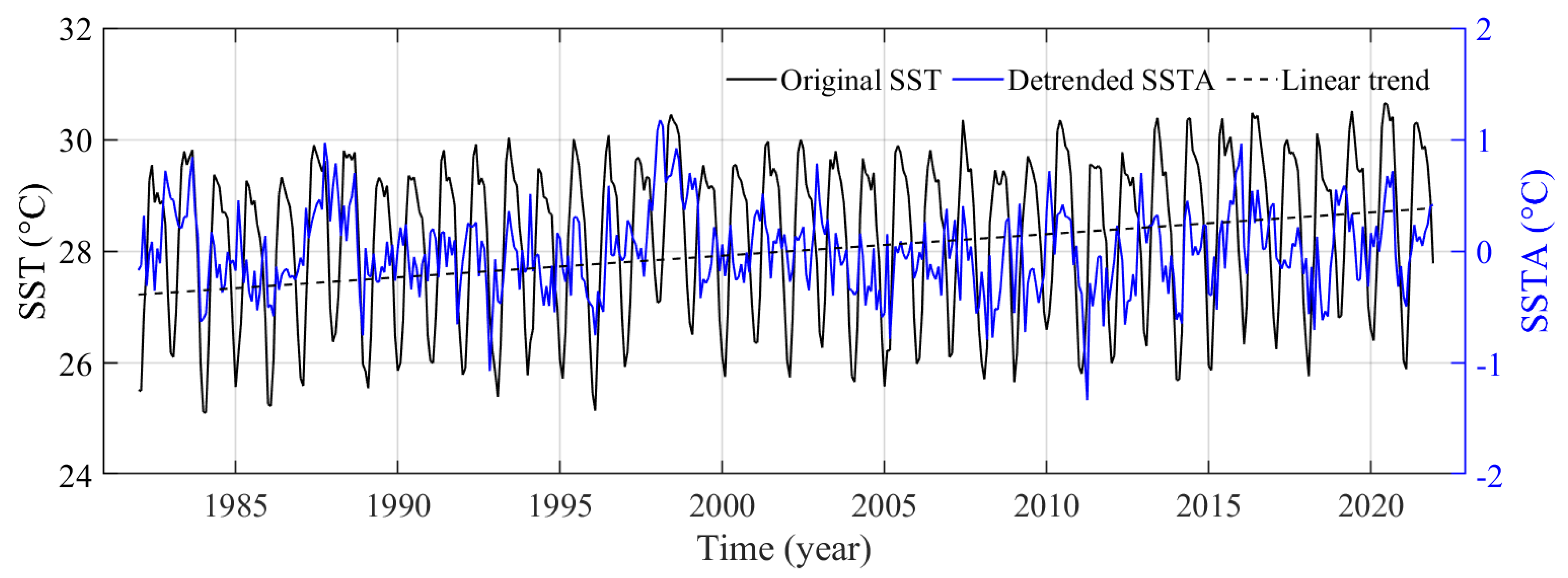
Figure 1. Monthly SSTA and detrended SSTA averaged over SCS during 1982–2021. The warming linear trend (black dashed line) is shown.
Remotesensing 16 01034 g001
Figure 2. Flowchart of the hybrid predictive model using one of the neural networks of BP, LSTM and GRU.
Remotesensing 16 01034 g002
Figure 3. Averaged (a) MAEs (°C), (b) RMSEs (°C) and (c) ACCs for the SCS SSTA forecasts at lead times of 1–50 days generated by persistence (dark blue bars), BP (yellow bars), LSTM (green bars), and GRU (light blue bars). The black dashed line in (a,b) indicates the climatology (~0.61 °C and ~0.75 °C) of the basin-wide SSTA for the period 1982–2021, and the black dashed line in (c) is an ACC of 0.6, which is a rule of thumb for measuring “usefulness” of predictions.
Remotesensing 16 01034 g003
Figure 4. Boxplot of bias (°C) in the daily SCS SSTA forecasts produced by the BP model as a function of forecast lead time for the period 2015–2021. The box and whiskers show the interquartile range and 99% confidence intervals, with circles above and below the whiskers representing the outliers. The central line and dot within the box denote the mean value and median, respectively.
Remotesensing 16 01034 g004
Figure 5. Daily RMSEs (°C; a,b) and ACCs (c,d) of the SCS SSTA forecasts produced by the BP model (a,c) and persistence (b,d) at lead times of 1–50 days for the period 2015–2021. The blank areas in (a,b) indicate RMSEs are larger than the climatology (~0.75 °C), and those in (c,d) indicate ACCs smaller than the threshold of 0.6. Black arrows at the top panel point to the blanks.
Remotesensing 16 01034 g005
Figure 6. Correlation coefficients, computed as a function of forecast length for the period 2015–2021, between RMSE and ACC derived from the BP model (black solid line) and persistence (black dashed line), and for RMSE (blue solid line) as well as ACC (blue dashed line) derived from the BP model and persistence.
Remotesensing 16 01034 g006
Figure 7. Maps of monthly SSTA climatology (°C; the first row) and RMSE (°C; the second to last row, excluding the first panel in the second row, which is the annual SSTA climatology) for SCS SSTA forecasts by the BP model at a lead time of 50 days in each year for the period 2015–2021. The black contour indicates the value of ~0.75 °C corresponding to the mean value of the annual SSTA climatology for the entire SCS basin.
Remotesensing 16 01034 g007
Figure 8. (Top and middle) Composite map of the forecast skill horizon for each year when the monthly RMSE of the model forecasts in each grid crosses the corresponding monthly climatological RMSE during the period 2015–2021. (Bottom) Frequency distribution (%) for the numbers of grids with the monthly RMSE of the model forecasts for the SCS basin less than the corresponding monthly climatology at lead times of 1–50 days during the period 2015–2021.
Remotesensing 16 01034 g008
Figure 9. (Left) Wavelet power spectrum (shading) of the daily forecast skill horizon determined by the ACC threshold of 0.6. Cone of influence is shown by the solid line. (Right) Global wavelet spectrum (solid curve) calculated by the time average of the wavelet power spectrum. The dashed lines in both panels represent the 95% confidence level for a red-noise process.
Remotesensing 16 01034 g009
Figure 10. Monthly mean (a) and 12-month running mean ACCs (c) of the forecasts produced by the BP model at lead times of 1–50 days for the period 1982–2021. Monthly mean ACCs of the persistence at lead times of 1–5 days are given in (b). The purple solid and dashed lines in (c) represent the basin-wide averaged monthly SSTA and Niño 3.4 index, respectively. Those with ACCs smaller than the threshold of 0.6 are indicated by the blank area. (d): Seasonally dependent temporal persistence of SSTAs starting in December, March, June, and September, respectively, calculated by correlating SSTAs from the 1st to the final day of each month with the SSTAs on subsequent days over a 30-day period across all years by using a correlation threshold of 0.6 [26,27].
Remotesensing 16 01034 g010
Figure 11. Basin averaged RMSEs (°C; rising lines) and ACCs (descending lines) for SCS SSTA forecasts at lead times of 1–50 days generated by the model under normal (solid lines) and severe (dashed lines) weather conditions for the period 2015–2021.
Remotesensing 16 01034 g011
Figure 12. SST changes (°C) in the truth (top) and forecast (middle) and the forecast error (bottom) on the day when the typhoon reaches its peak intensity over the 50-day forecast window. Thick black line shows typhoon track, and colored circles denote typhoon intensity. Time when typhoon reaches its peak intensity is labeled in the form of two-digit month and day (i.e., mmdd) in each top panel.
Remotesensing 16 01034 g012
Disclaimer/Publisher’s Note: The statements, opinions and data contained in all publications are solely those of the individual author(s) and contributor(s) and not of MDPI and/or the editor(s). MDPI and/or the editor(s) disclaim responsibility for any injury to people or property resulting from any ideas, methods, instructions or products referred to in the content.