Abstract
Pan-sharpening is a fusion process that combines a low-spatial resolution, multi-spectral image that has rich spectral characteristics with a high-spatial resolution panchromatic (PAN) image that lacks spectral characteristics. Most previous learning-based approaches rely on the scale-shift assumption, which may not be applicable in the full-resolution domain. To solve this issue, we regard pan-sharpening as a multi-task problem and propose a Siamese network with Gradient-based Spatial Attention (GSA-SiamNet). GSA-SiamNet consists of four modules: a two-stream feature extraction module, a feature fusion module, a gradient-based spatial attention (GSA) module, and a progressive up-sampling module. In the GSA module, we use Laplacian and Sobel operators to extract gradient information from PAN images. Spatial attention factors, learned from the gradient prior, are multiplied during the feature fusion, up-sampling, and reconstruction stages. These factors help to keep high-frequency information on the feature map as well as suppress redundant information. We also design a multi-resolution loss function that guides the training process under the constraints of both reduced- and full-resolution domains. The experimental results on WorldView-3 satellite images obtained in Moscow and San Juan demonstrate that our proposed GSA-SiamNet is superior to traditional and other deep learning-based methods.
1. Introduction
With the launch of a lot of earth observation satellites, multi-spectral (MS) images play an important role in agriculture, disaster assessment, environmental monitoring, land cover classification, etc. The ideal MS images are acquired at multiple wavelength bands with high spatial resolution. However, limitations include the incoming radiation energy and the volume of data collected [1], but one solution can be found by obtaining two kinds of images: a high-spatial resolution panchromatic (HR PAN) image and an MS image with fewer spatial details. These images contain both redundant and complementary information; hence, pan-sharpening, which refers to the fusion of a PAN image and an MS image to produce an HR MS image of the same size as a PAN image, has received significant attention, [1,2].
Numerous endeavors have been dedicated to the development of pan-sharpening algorithms in the past few decades. For conventional techniques, there are three categories: component substitution (CS) methods, multi-resolution analysis (MRA) approaches, and variational optimization-based (VO) techniques. The CS methods inject spatial information by displacing components with PAN images. The most well-known algorithms are intensity–hue–saturation [3], principal component analysis [4], Brovey transforms [5], and Gram–Schmidt spectral sharpening [6]. The two types of methods could have low computational costs and promising outcomes but sometimes may suffer from spectral distortions. The MRA approaches assume spatial details can be obtained through a multi-resolution decomposition of the PAN image. The injection of high frequencies from PAN images to the MS bands improves the spatial resolution. On the basis of the different decomposition algorithms, the MRA methods comprise the decimated wavelet transform [7], the smoothing filter-based intensity modulation [8], à trous wavelet transform (ATWT) [9], contourlet [10], etc. Compared to the CS and MRA approaches, VO-based approaches are relatively new. Methods in this category always consider the observed MS images as degraded versions of an ideal HR MS image. Based on this assumption, the recovery results for HR MS images can be obtained using the optimization algorithm. Representative methods include model-based fusion using PCA and wavelets [11], the sparse representation of injected details [12], and model-based, reduced-rank pan-sharpening [13]. VO-based techniques can yield competitive results, but a large number of hyperparameters and insufficient feature representation could result in spatial and spectral distortions.
Over the past few years, deep learning has become more in vogue, and scholars have attempted to explore the high nonlinearity of convolutional neural networks (CNNs) in the context of the pan-sharpening problem. In PNN [14], the results are pan-sharpened by a simple CNN with a structure similar to that of a super-resolution CNN (SRCNN) [15]. Ref. [16] is similar to that of a PNN, and the difference is that the network is used to super-resolve MS images in HIS space; then, the MS and PAN images are further enhanced by GS transform to accomplish the pan-sharpening. TFNet [17] first fuses the MS and PAN images in the feature level, and then the pan-sharpened images are reconstructed from the fused features. Yang et al. [18] propose a deep network architecture called PanNet for pan-sharpening. The network learns the residuals between the up-sampled MS image and the HR MS image. The training process operates within the domain of high-pass filtering. PSGAN [19] introduces the generative adversarial network (GAN) to produce high-quality pan-sharpened images. MSDCNN [20] adds multi-scale modules on basic residual connections, and SRPPNN [21] utilizes high-pass residual modules to inject more abundant spatial information. Multi-scale structured sub-networks are used for the fusion of spatial details in LPPN [22]. These networks are trained under a complete supervision framework in a reduced resolution domain. The parameters that have converged are then utilized to fuse the target full-resolution PAN/MS images. Obviously, there is a gap between the assumption and the actual situation. For this reason, the above-mentioned methods exhibit satisfactory performance in the reduced resolution domain; however, they cannot ensure optimal performance in the target domain.
Valuable efforts have been made by other groups to overcome the deterioration in the generalization ability due to scale-shift. Ref. [23] proposes a dual-output and cross-scale strategy in which each sub-network is equipped with an output terminal that generates reduced- and target-scale results, respectively. However, its weakness is that it involves separate training processes and cascaded sub-networks, which make it computationally inefficient. PancolorGAN [24] applies data augmentation in the training by randomly varying the down-sampling ratios. Some GAN-based models, such as Pan-Gan [25], PercepPAN [26] and UCGAN [27], introduce unsupervised architectures to avoid scale-shift assumptions. Unsupervised learning architectures perfectly avoid the scale-shift issue; however, the training process of GANs is susceptible to vulnerabilities [28], which can lead to suboptimal outcomes.
The Siamese net [29] was initially introduced as a solution for addressing signature verification as an image-matching problem. This Siamese neural network architecture consists of two identical feed-forward sub-networks that are tied by an energy function at the final layer. These parameters are shared between the sub-networks, which means the same networks correspond with the same parameter . Weight bundling ensures that two similar images cannot be mapped to different positions within the feature space. The input pairs are embedded as representations in a high-dimensional domain. Then, the similarity of the two samples is compared by computing the distance between the two representations through a cosine distance. The network is optimized by minimizing the similarity metric when input pairs are from the same category and maximizing it when they belong to different categories.
At present, there have been several studies applying Siamese networks to solve pan-sharpening problems. In [30], the Siamese network is applied in a cascade up-sampling process in which multi-level local and global fusion blocks share network parameters. The intermediate-scale MS image outputs are used as part of the loss function. This method employs a Siamese fusion network to preserve the cross-scale consistency, but it still remains shifted with full-resolution domain. Ref. [31] proposes a knowledge distillation framework for pan-sharpening, aiming to imitate the ground-truth reconstruction process in both the feature space and the MS domain. The student network has the same architecture as the teacher network, and loss terms are applied in two intermediate feature layers. CMNet [32] combines the classification and pan-sharpening networks in a multi-task learning way. The pan-sharpening network performs better under the guidance of the classification network. It learns ideal high-resolution MS images from an application-specific perspective but introduces additional labels that are not easily accessible.
The scale-shift issue created by the lack of ground-truth in the full-resolution domain is still a challenge for deep-learning based methods. Thus, we propose a Siamese architecture named GSA-SiamNet equipped with a multi-resolution loss function. In Figure 1, we also perform a comparison of common network architectures and our Siamese design. We could divide the previous network architectures into two main categories. One takes reduced-resolution MS images as inputs, or up-samples them first, and then stacks them with the PAN images. The networks learn a mapping function using original MS images. The other category is the two-stream network, which fuses the PAN and MS images in the feature domain. Some researchers still train the pan-sharpening mapping function using reduced-resolution images. However, unsupervised approaches, such as GANs, are trained in the full-resolution domain, and their training processes are susceptible to vulnerabilities. Compared to the previous methods, we consider pan-sharpening to be a multi-task problem that aims to retain information in both the reduced- and full-resolution domains. We adopt the Siamese network and take both a reduced-resolution image pair and a full-resolution image pair as inputs. It is worth noting that our approach differs slightly from conventional Siamese networks. Instead of using a similarity constraint for the last layer, a multi-resolution loss function is designed for both the reduced- and full-resolution domain to preserve spectral and spatial consistency. The details are illustrated in Figure 2.
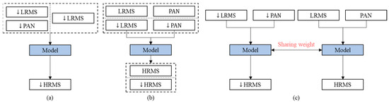
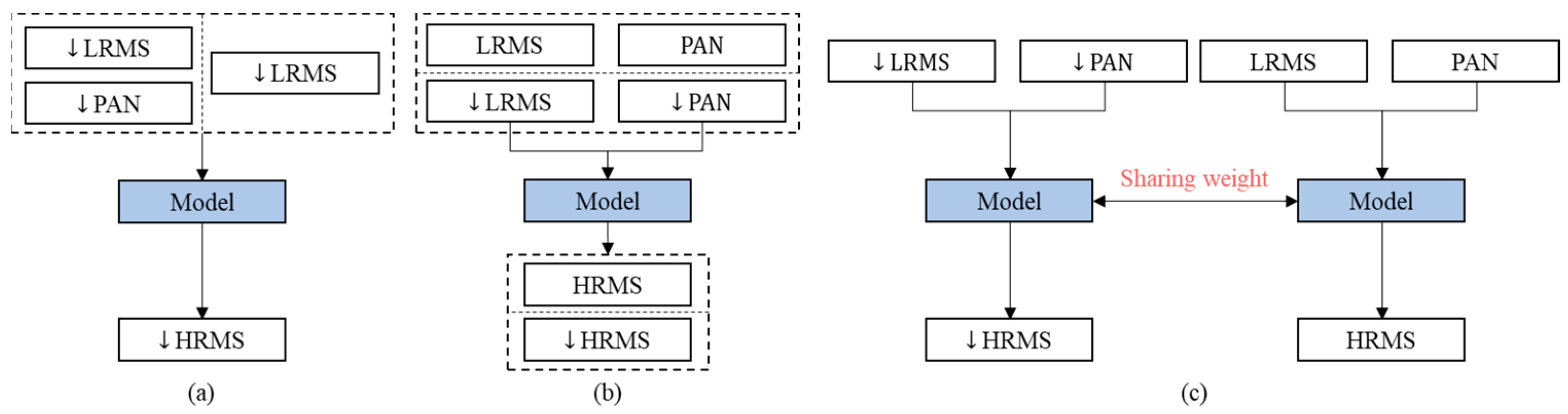
Figure 1.
The architecture of different networks for pan-sharpening in training. ↓ denotes that the images are in the reduced-resolution domain. Dashed borders represent independent samples of different resolutions. (a) The model has single input which is MS only or stacks both MS and PAN images. (b) The network has a two-stream structure, and original MS and PAN images are usually used in GAN-based models. (c) The Siamese architecture is our GSA-SiamNet that constrains the training process in both reduced- and full-resolution domains.
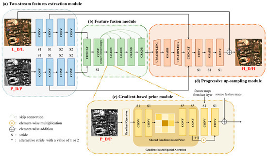
Figure 2.
Architecture of our GSA-SiamNet for pan-sharpening. L_D, P_D, and H_D denote the reduced-resolution MS image, PAN image, and the corresponding fused HR MS image; L, P, and H denote the original full-resolution images.
The major contributions of this paper are summarized as follows. First, we propose a Gradient-based Spatial Attention (GSA) module to optimize the injection process of spatial information in multi-level intermediate layers. The high-pass information is extracted by gradient operators. Then, learned gradient-based prior is shared as the input. Here, we utilize gradient-based prior as a spatial attention mask to guide texture recovery for different regions (with different levels of spatial details). Second, a multi-resolution loss function is designed to constrain the network training in both the reduced- and full-resolution domains. Full-resolution pan-sharpening, as an auxiliary task, markedly improves the pan-sharpening performance, and the reduced-resolution pan-sharpening task supports spectral consistency. The multi-task strategy helps GSA-SiamNet achieve better scale-shift adaptation compared to other approaches.
This paper is organized as follows. In Section 1, we provide a detailed comparison with previous learning-based network architecture and introduce the background of Siamese architecture. We propose a novel GSA-SiamNet architecture and give details in Section 2. Section 3 describes experiments, followed by a series of comparisons with other methods. The conclusion and discussion are provided in Section 4.
2. Materials and Methods
In this section, we give a detailed description of our method. For convenience, we denote the original MS and PAN images as and , where , , and respectively denote the width, height, and the number of channels of the MS image, while and are the width and height of the PAN. The ratio of spatial resolution between MS and PAN images is defined as . The reduced-resolution MS and PAN images are represented as and , whose resolution also satisfies the above relationship. The pan-sharpened HR MS image has both high spectral and spatial resolutions.
The pan-sharpening task is to reconstruct high-quality MS images with both advantages of PAN and MS images. A general formulation of the deep learning-based approaches can be defined as:
where the subscript denotes the th spectral band, and indicates the upscaling version of the th band of . denotes the detail extraction function learned by the network. Most state-of-the-art methods treat the function as minimizing an objective of the form:
where enforces spectral consistency, enforces structural consistency, and is other possible image constraints on sharpened MS images.
2.1. Network Architecture
PAN and MS images focus on preserving both geometric details and spectral information. Unfortunately, there is no well-defined boundary between spatial and spectral information. Those undesirable pan-sharpened results are caused by redundant spectral information on flat regions or insufficient extraction of spatial characteristics at edges. Furthermore, the single-resolution loss function, which treats the original MS images as the ground truth, overlooks the importance of PAN images. Motivated by this fact and the fact that the complexity of enhancing the image varies spatially, we propose a GSA-SiamNet for pan-sharpening. In this section, we introduce the four key components shown in Figure 2. Because of the symmetry of the Siamese network, we just describe the full-resolution image pairs as inputs in the next paragraphs.
2.1.1. Two-Stream Features Extraction Module
In this paper, we use a two-stream network as a generator to generate pan-sharpened images [19]. Instead of directly stacking PAN and MS images [25], we accomplished fusion in the feature domain, which has proved to reduce spectral distortion [33]. One sub-network took a multi-band up-sampled MS image as input, while the other sub-network took a single-band PAN image. In both sub-networks, there were four convolutional layers with convolutional kernels used to extract the features. The stride of the first two layers is 1, and for the rest, it is 2 in order to compress the features. All of the convolution layers were activated through the Leaky Rectified Linear Unit (Leaky ReLU) with a slope of 0.2.
2.1.2. Feature Fusion Module
This module enables the proper fusion of PAN and MS images in the feature space. Instead of a cascade connection, we introduce a skip connection method which shares the source features [34] among Gradient-based Spatial Attention Dense Blocks (GSADBs). The residual function of layer is:
where refers to the feature maps from the first convolution layer of this module and is set to 4 in this study. Each layer, called a Gain Block (GB), consists of two convolution layers with a Leaky ReLU activation function and is adjusted via a GSA mask. By simply multiplying these two vectors together, we can adaptively amplify the pairs with high spatial correlation and enhance the network’s ability to capture valid features. The details can be written as:
where denotes the convolutional layer with kernel, is spatial attention features (see the following section for detailed descriptions), and denotes Leaky Rectified Linear Unit activation layer. is the feature-map of the GSADBs of the GBs. The end of the fusion module is a tensor that encodes both spatial and spectral features.
2.1.3. Gradient-Based Spatial Attention Module
As part of feature fusion module, this GSA module is a flexible plugin that generates spatial attention features and refines the intermediate features within GSADBs. The high-pass information extracted from the PAN image has been used in many variational methods, and it has been shown to be effective in enforcing structural consistency. We no longer use high-pass information as a constraint in the loss function, which is different from the above variational methods. First, we utilize Laplacian and Sobel operators to obtain high-pass information from PAN images as attention prior. These gradient maps guide texture recovery for different regions. Second, the gradient-based prior helps to capture delicate texture. Through learning the GSA, we obtain a spatial attention mask that enhances spatial texture and inhibits the distortion to original spectral information in flat regions. The feature fusion module becomes more sensitive to spatial details in edge regions and less disruptive to spectral characteristics of smoothing regions.
In detail, we employ gradient maps as input and then employ a two-layer branch to generate a gradient-based prior, which is shared among GSA modules within the same stages. We set the size of the convolutional kernel to 3 and the stride to 1. However, we vary the kernel size to 4 and the stride to 2 to align the size of the attention masks and features. Then, a shared gradient-based prior performs forward passes through two successive convolutions to capture spatial attention .
2.1.4. Progressive Up-Sampling Module
Fusion features are progressively up-sampled to the PAN image size with two sub-pixel convolution layers, which can learn parameters for the upscaling process. Each up-sampling branch is also followed by a local residual block with a GSA module to modify features. The skip concatenation will help inject the details into higher layers, thereby noticeably easing the training process. A flat convolutional layer is applied last to generate the final residual of the up-sampled MS and the ideal HR MS . This global residual learning [35] avoids the complicated transformation from input image pairs to targets and simply requires learning a residual map to restore the missing high-frequency details.
2.1.5. Loss Functions
In this paper, we decompose pan-sharpening into two sub-problems and regard it as a multi-task problem. The multi-resolution loss function is proposed, aiming to retain both spectral and spatial information at different resolution scales. It is defined as follows:
where is the coefficient to balance different loss terms, which is set to 0.1 in this paper. The first term measures the pixel-wise difference between the spectral information of the fused HR MS image with reduced-resolution and that of the original MS image, as follows:
where is the size of a train batch. Although loss has been widely used in this term, the loss function can lead to a local minimum, which makes the performance of our model unsatisfactory in flat areas [17]. Here, we adopt loss to measure the accuracy of the network’s reconstruction.
The second term measures difference in gradients between the generated full-resolution HR MS image and the original PAN image, which is defined as follows:
where denotes the gradient operator using the Laplacian operator and is an average pooling along the channel dimension. This loss function takes advantage of the PAN image and gives a spatial constraint at a higher resolution.
3. Experimental Results and Analysis
In this section, we compare the proposed GSA-SiamNet with six widely used techniques: AWLP, MTF-GLP, BDSD, PCNN, PSGAN, and LPPN. All the codes of these compared methods are publicly available [2], and we train them on our datasets with the default parameters. Here, we use [36], [37], [38], [39], and [40] to evaluate the performance of the proposed method. The metrics , , and , which do not need reference images, are employed in full-resolution validation.
3.1. Datasets
To validate the performance of the proposed method, a WorldView-3 (WV-3) Dataset was used for the pan-sharpening experiments. The number of spectral bands is 8 (coastal, blue, green, yellow, red, red edge, near-IR1, and near-IR2) for the MS image taken from WV-3 sensors. Sensors carried by the WV-3 satellite can acquire MS images with a spatial resolution of 1.24 m and PAN images with a resolution of 0.31 m. The WV-3 dataset used in this paper is collected by the DigitalGlobe WV-3 satellite over Moscow and San Juan. The images from these three regions were acquired at different times and also differ significantly in their geographical settings.
3.2. Implementation Details
The mini-batch size is set to 16. The parameters in our GSA-SiamNet are updated by the Adam optimizer. The GSA-SiamNet is implemented in PyTorch and trained in parallel on two NVIDIA GeForce GTX 1080 GPUs. Then, the original MS and PAN images are used as the ground truth for spectral and spatial constraints. The size of the raw MS images is and that of the PAN images is the corresponding . The training set, collected from Moscow and Mumbai, includes 2211 samples, and one-tenth is used as the validation. There are 399 images used for the test that were collected over Moscow and San Juan. The number of epochs trained is controlled by early stopping.
3.3. Ablation Study
3.3.1. Evaluation of GSA
The GSA module can be stacked flexibly at any stage of the pan-sharpening process. As shown in Figure 3, we conducted an experiment to show the effectiveness of the GSA module. By varying its integration position, we evaluate the contribution to each stage. For a fair comparison, we compare them to architectures of the same depth that do not include GSA. The skip connection residual block in the feature fusion module is also replaced with a single convolution operator. In Table 1, bold represents the best result. The average values and standard deviations of each station are listed. From a quantitative perspective, the network’s performance is improved to different degrees, regardless of the stage of module insertion. In particular, the three metrics ( , and PSNR) are optimal when the module is inserted in the image fusion phase, while the remaining two metrics are suboptimal. These results indicate that our GSA layer indeed leads to valid performance improvement and improves the network’s ability to handle spatial details with less spectral loss. In this paper, the complete GSA-SiamNet inserts these GSA modules into all stages.
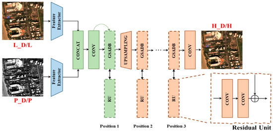
Figure 3.
Evaluation of GSA. By varying its integration position, we evaluate the contribution in each stage. For a fair comparison, the skip connection residual block in the feature fusion module is replaced by a single convolution operator to maintain the same depth. The network uses the concatenation operation and residual structure as GSA-SiamNet in Figure 2 but omits them in this figure.

Table 1.
Quality metrics at a reduced resolution of different portions of the GSA module applied to the whole test datasets.
3.3.2. Evaluation of Number of Recursive Blocks
Because of weight-sharing sets among the residual units within a recursive block, the parameter volume remains the same as the layers of the network become deeper. As shown in Figure 4, we explore various combinations of F, U, and R to construct models at different depths and observe how these three parameters affect the performance. Here, F, U, and R represent the number of recursions of GSADB at each stage.
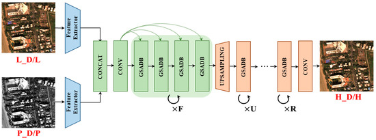
Figure 4.
Evaluation of number of recursive blocks. F, U, and R denote the number of recursive blocks in the image fusion, up-sampling, and reconstruction stages. The network uses the concatenation operation and residual structure as GSA-SiamNet in Figure 2 but omits them in this figure.
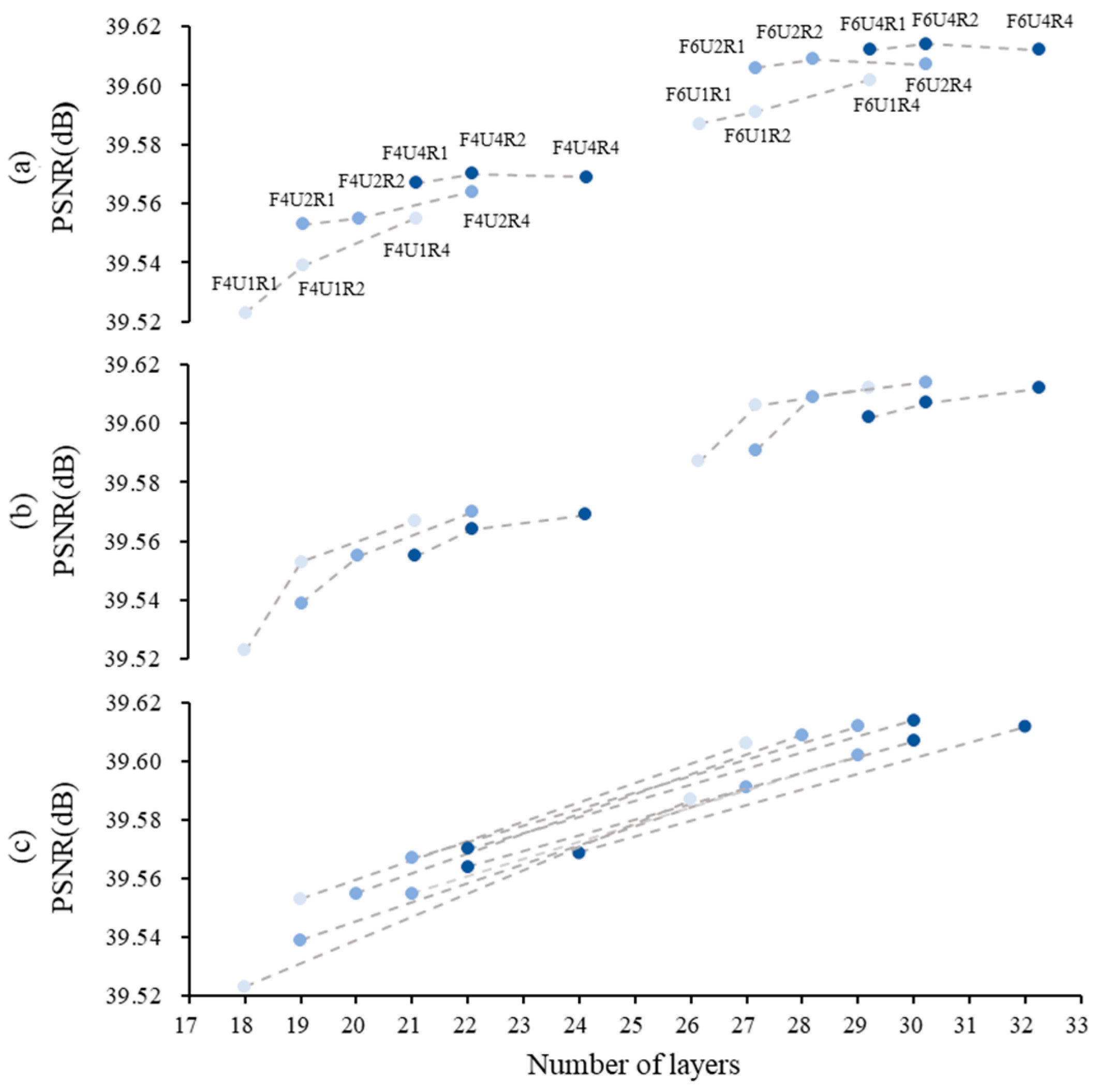
To clearly show the impact of the number of recursive blocks, we plot three sets of line graphs in Figure 5. The experiment was divided into two groups (setting and ). The data in these three subplots are the same, but we have connected the results of the fixed recursive number in different stage situations with dashed lines. For example, we connect the results of the same number of U in subplot (a). The darker color of the dots represents the larger recursive number in the group.
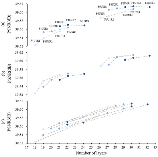
Figure 5.
PSNR of various GSA-SiamNet structures at different combinations of F, U, and R. The experiment is divided into two groups, with settings F = 4 and F = 6. Dots of darker color represent the larger recursive number in the inner group. (a) The results are connected by points with the same number of U in both groups. (b) The results are connected by points with the same number of R in both groups. (c) The results are connected by points with the same number of F between groups.
Figure 5 shows that increasing the recursion number makes the network deeper and achieves better performance, indicating that deeper networks are generally better. In terms of intra-group comparisons, we fixed the parameter at 4 or 6 and observed that increasing resulted in a greater performance improvement compared to increasing when the depth was the same. For example, (d = 15) and (d = 16) achieve 39.54 and 39.55 dB. The performance gains diminish as depth increases: (d = 16) and (d = 16) are two obvious turning points. In addition, the slope of the fold in (b) is greater compared to that in (a). We prefer to use our GSA module in shallower layers.
When making comparisons between groups, the performance improvement is less pronounced as the depth increases, specifically in the case of is 6. This result is consistent with previous findings. Despite the different depths, the three networks achieve comparable performances (, d = 6, 39.612 dB; , d = 6, 39.614 dB; , d = 5, 39.612 dB) and outperform the previous shallow networks. Under this recursive learning strategy, can achieve state-of-the-art results.
3.4. Reduced-Resolution Validation
Following Wald’s protocol [41], we evaluate the methods at reduced resolution. This means that the original MS and PAN images are filtered by a Gaussian blur kernel and are further down-sampled using the nearest neighbor technique with a factor of ). Five widely used metrics, including , sCC, SAM, ERGAS, and PSNR, are used to assess the quantitative comparison of the proposed method.
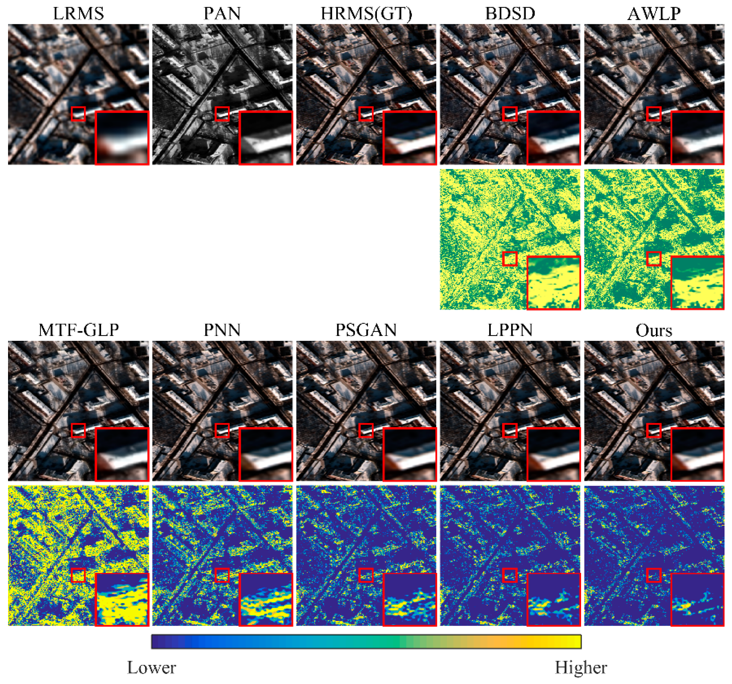
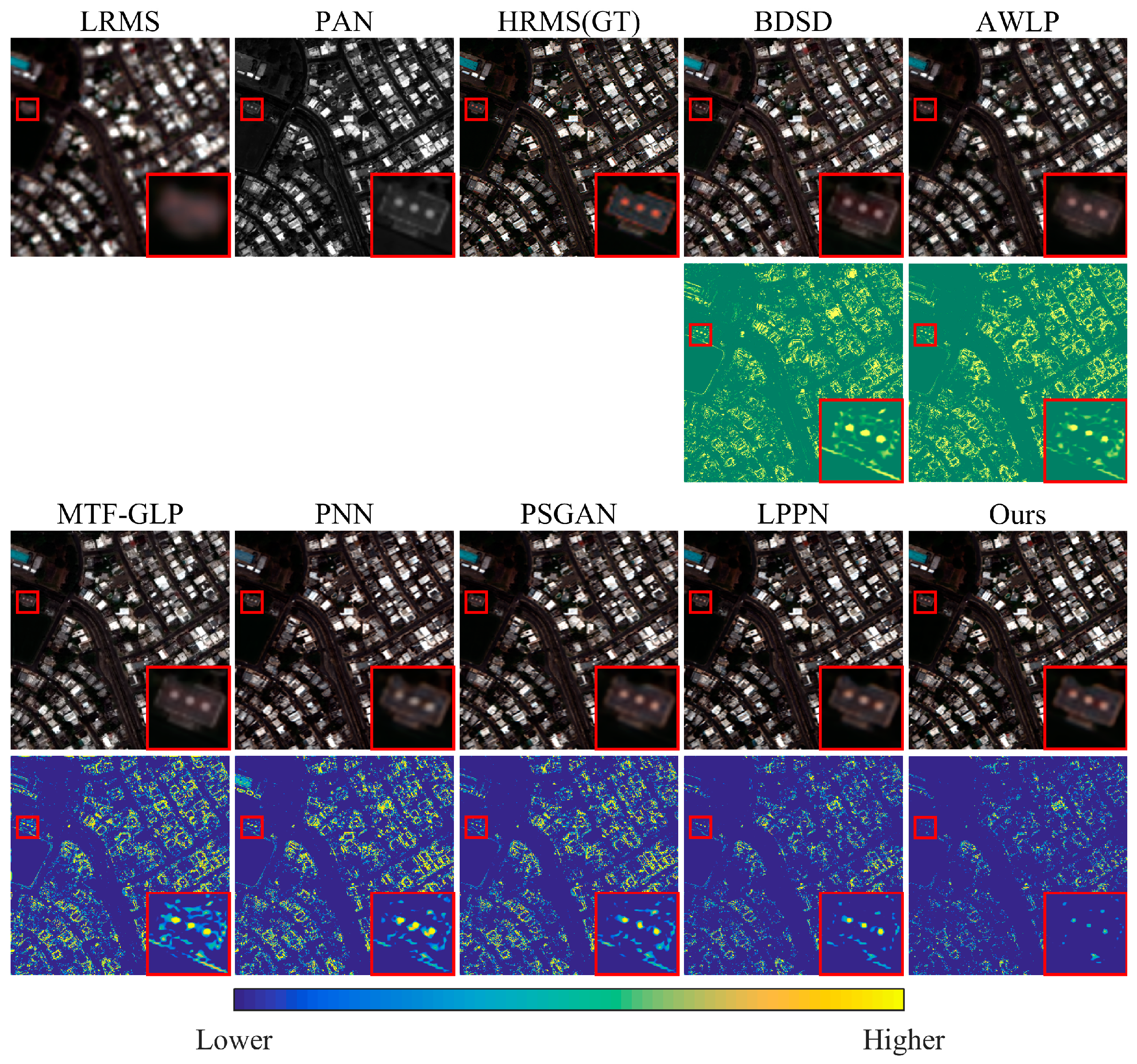
The results of the fusion are shown in Figure 6 and Figure 7. The first row shows the up-sampled LR MS, PAN, original HR MS (GT), and fusion results in which all MS images are displayed in true color (RGB). The second row comprises the corresponding error images, which regard the original MS image as ground truth. We color-coded the error image according to the color bar at the bottom of the figure. We performed an exponential transformation on the error image for clear visual effects. A truncated value was used to prevent small errors from being missed. From left to right, the colors represent the values from minimum to maximum.
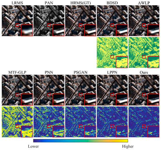
Figure 6.
Qualitative comparison of the data from Moscow using the reduced-resolution test. The first row displays the fusion results in true color (RGB), and the second row shows the corresponding error images, which regard the original HRMS as the ground truth. We apply an exponential transformation to the error image to enhance visual clarity. The red boxes mark the regions of interest and the corresponding zoomed-in images.
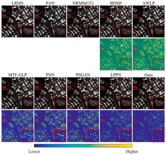
Figure 7.
Qualitative comparison of the data from San Juan using the reduced-resolution test. The first row displays the fusion results in true color (RGB), and the second row shows the corresponding error images, which regard the original HRMS as the ground truth. We apply an exponential transformation to the error image to enhance visual clarity. The red boxes mark the regions of interest and the corresponding zoomed-in images.
In Figure 6 and Figure 7, the geometric details are effectively preserved in the reduced-resolution domain but have drawbacks, such as spectral distortion. Overall, the error plots show significant spectral distortions in BDSD and AWLP. Three conventional methods are too simple and brutal for the injection of high-frequency information, and the generated results perform poorly in terms of spectral consistency. PNN, PSGAN, LPPN, and our GSA-SiamNet have lower errors than the traditional methods. Learning-based injection functions have an advantage over manually designed injection functions in terms of spectral preservation. In Figure 7, the colored ground objects suffer from varying degrees of spectral information loss in all pan-sharpened images. Among these methods, our method has the smallest mean error. Our GSA-SiamNet maintains a smaller distortion of the spectrum in the low-frequency regions and selectively injects high-frequency information.
Quantitatively, Table 2 lists the results of the two sub-datasets. In the table, the best result is represented in bold. It can be observed that learning-based pan-sharpening methods outperform traditional approaches. Among the learning-based approaches, our GSA-SiamNet can yield a better performance than all the other competitors in all metrics. This is consistent with the conclusions obtained in the qualitative comparison. Consequently, our GSA-SiamNet can generate the closest fusion result to the reference MS (the ground truth), both spectrally and spatially. Regardless of qualitative or quantitative comparisons, our proposed method always yields a satisfactory performance.
Table 2.
Quality metrics at the reduced-resolution of different methods on two sub-datasets.
3.5. Full-Resolution Validation
We also evaluate the algorithms at the full resolution of the images. In this case, three no-reference metrics (QNR, , and ) are calculated on full-resolution images.
The quantitative values in Table 3 indicating the best performance are marked in bold. It is worth mentioning that the GSA-SiamNet does not achieve the best performance in every metric. The validation at full resolution allows for the avoidance of unknown ground truth, but the values of the indexes are less reliable because they heavily rely on the up-sampled MS image. In other words, visual evaluation is more reliable than quantitative evaluation in the full-resolution experiment.
Table 3.
Quality metrics at the full-resolution of different methods on two test datasets.
Furthermore, we exhibit the average inference time for each fusion method, denoted as A.T., in seconds, in Table 4. Traditional methods run on CPUs, while deep-learning based methods perform inferences on GPUs. Since the two run in different environments, we only compare the computation cost of the deep-learning based methods. For the average inference time of test datasets, the PCNN has the shortest inference times, while LPPN and our GSA-SiamNet have slightly higher computational costs. The recursive structure makes the network deeper so that it achieves better performance but increases inference time. In the future, we will study the optimization algorithm to improve computational efficiency.
Table 4.
The average inference time for test datasets.
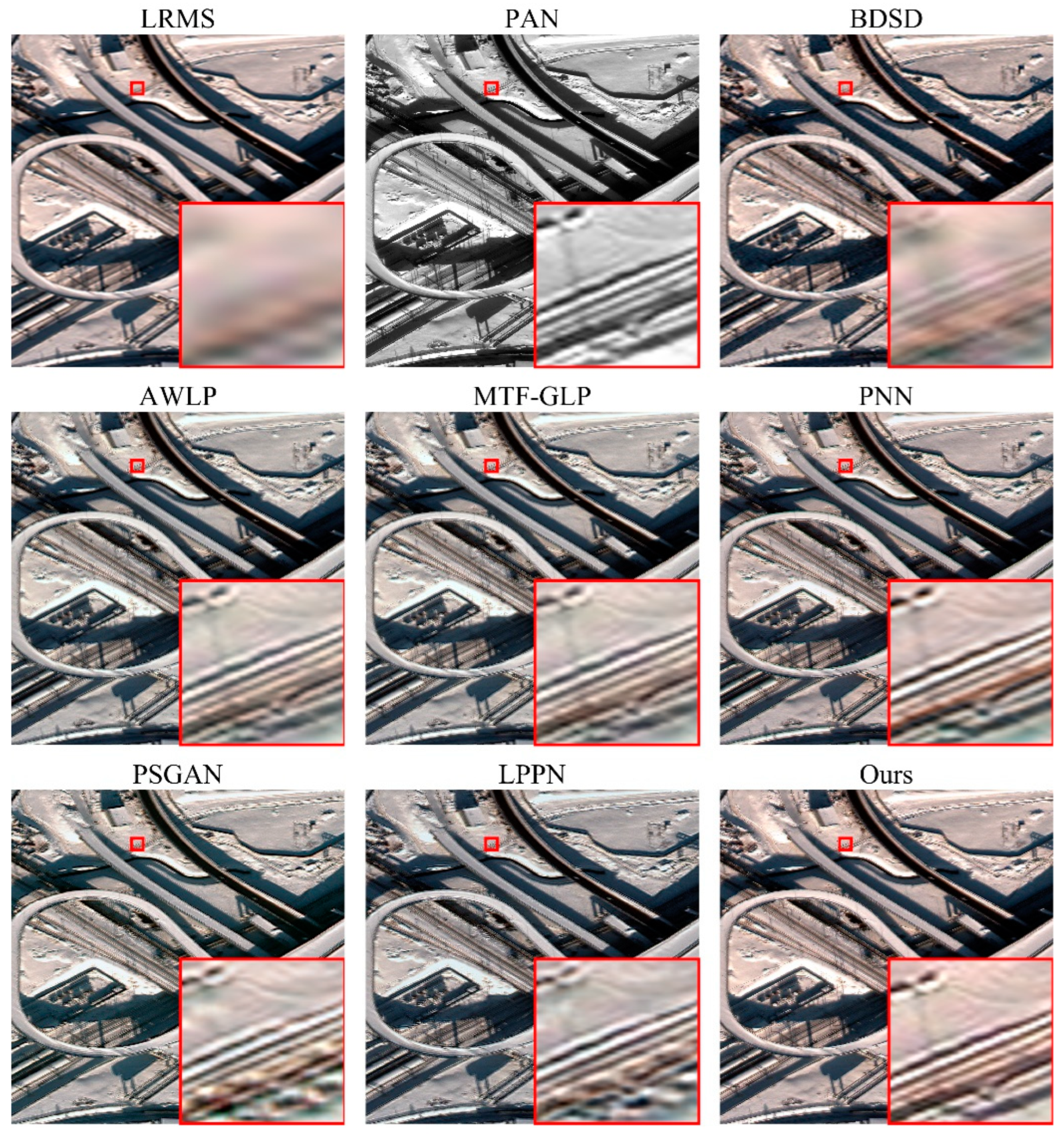
As shown in Figure 8 and Figure 9, we select a typical example of the results from each dataset. Discrepancies between the quantitative metrics and the visual appearance of the results can be observed. In Figure 8, BDSD has the worst results, with the complete distortion of details. The localized, zoomed-in views show that PSGAN and LPPN failed to recover the spatial characteristics, and the image appears distorted at the edges. AWLP, MTP-GLP, PNN, and our method can maintain the details, which are as clear as those in the PAN image, well. Overall, only BDSD, PNN, and our method retain the spectral features of the original image on the snow surface. Figure 9 is a sample collected from San Juan, and its distribution is significantly different from that of the training set. In the localized, zoomed-in views, the original LRMS yield jagged edges, which leads to severe artifacts in BDSD and AWLP. PSGAN and LPPN yield spatial distortions, while MTF-GLP and our GSA-SiamNet perform well from an anti-aliasing perspective. When the distribution of the test data differs from the distribution of the training data, PNN, PSGAN, and LPPN lose the advantage of spectral preservation and introduce some blurred information into the result. MTF-GLP suffers from color distortion. In this full-resolution validation, the pan-sharpened HR MS generated by GSA-SiamNet is visually superior.
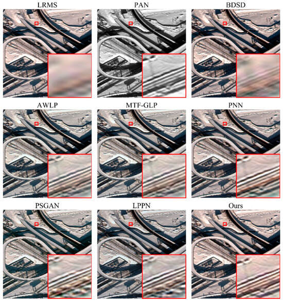
Figure 8.
Qualitative comparison using the full-resolution test on the data from Moscow. The red boxes mark the regions of interest and the corresponding zoomed-in images.
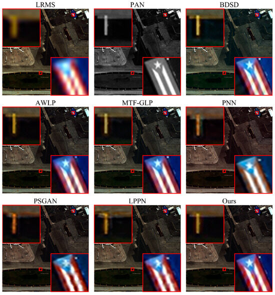
Figure 9.
Qualitative comparison using the full-resolution test on the data from San Juan. The red boxes mark the regions of interest and the corresponding zoomed-in images.
In this section, we show the superiority of our GSA-SiamNet at full resolution. Thanks to our GSA-SiamNet’s focus on high-frequency content, it is more robust compared to other networks. As a result, the network can effectively translate a superb training performance to an excellent testing performance on new images with different distributions.
4. Conclusions
In this article, we regard pan-sharpening as a multi-task problem and propose a GSA-SiamNet that takes both the original MS/PAN images and down-sampled MS/PAN images as inputs. To address the issue of model performance degradation caused by the scale-shift assumption, a multi-resolution loss function is designed to guide the training process in both the reduced- and full-resolution domains. Down-sampled inputs focus on spectral consistency, while another one is used for generating spatial consistency. In ablation analysis, we validate the effectiveness and efficiency of GSA modules. This spatial attention effectively improves the network’s performance in the feature fusion, up-sampling, and image reconstruction stages. Experimental testing of two sub-datasets show that our GSA-SiamNet effectively preserves the underlying spectral information distribution while minimizing the loss of spatial information, outperforming current state-of-the-art methods.
Author Contributions
Methodology, data curation, writing—original draft, and writing—review & editing, Y.G.; writing—review & editing and supervision, M.Q.; writing—review & editing and supervision, S.W.; writing—review & editing and supervision, F.Z.; supervision, Z.D. All authors have read and agreed to the published version of the manuscript.
Funding
This research was funded by the National Key Research and Development Program of China (Grant No. 2021YFB3900900), the Provincial Key R&D Program of Zhejiang (Grant No. 2021C01031), and the China Postdoctoral Science Foundation (Grant No. 2022M720121). This research was also funded by the Deep-time Digital Earth (DDE) Big Science Program.
Data Availability Statement
The source code is available at https://github.com/isabel-gao/GSA-SiamNet.git, accessed on 23 October 2022. The WV-3 dataset used in this paper was downloaded from https://spacenet.ai/sn5-challenge/, accessed on 22 August 2019.
Conflicts of Interest
The authors declare no conflicts of interest.
References
- Zhang, Y. Understanding Image Fusion. Photogramm. Eng. Remote Sens 2004, 70, 657–661. [Google Scholar]
- Vivone, G.; Alparone, L.; Chanussot, J.; Dalla Mura, M.; Garzelli, A.; Licciardi, G.A.; Restaino, R.; Wald, L. A Critical Comparison among Pansharpening Algorithms. IEEE Trans. Geosci. Remote Sens. 2015, 53, 2565–2586. [Google Scholar] [CrossRef]
- Carper, W.; Lillesand, T.; Kiefer, R. The Use of Intensity-Hue-Saturation Transformations for Merging SPOT Panchromatic and Multispectral Image Data. Photogramm. Eng. Remote Sens. 1990, 56, 459–467. [Google Scholar]
- Shahdoosti, H.R.; Ghassemian, H. Combining the Spectral PCA and Spatial PCA Fusion Methods by an Optimal Filter. Inf. Fusion 2016, 27, 150–160. [Google Scholar] [CrossRef]
- Gillespie, A.R.; Kahle, A.B.; Walker, R.E. Color Enhancement of Highly Correlated Images. II. Channel Ratio and “Chromaticity” Transformation Techniques. Remote Sens. Environ. 1987, 22, 343–365. [Google Scholar] [CrossRef]
- Baier, T.; Dupeux, G.; Herbert, S.; Hardt, S.; Quéré, D. Propulsion Mechanisms for Leidenfrost Solids on Ratchets. Phys. Rev. E-Stat. Nonlinear Soft Matter Phys. 2013, 87, 021001. [Google Scholar] [CrossRef] [PubMed]
- Otazu, X.; González-Audícana, M.; Fors, O.; Núñez, J. Introduction of Sensor Spectral Response into Image Fusion Methods. Application to Wavelet-Based Methods. IEEE Trans. Geosci. Remote Sens. 2005, 43, 2376–2385. [Google Scholar] [CrossRef]
- Wald, L.; Ranchin, T. Liu “Smoothing Filter-Based Intensity Modulation: A Spectral Preserve Image Fusion Technique for Improving Spatial Details”. Int. J. Remote Sens. 2002, 23, 593–597. [Google Scholar] [CrossRef]
- Nunez, J.; Otazu, X.; Fors, O.; Prades, A.; Pala, V.; Arbiol, R. Multiresolution-Based Image Fusion with Additive Wavelet Decomposition. IEEE Trans. Geosci. Remote Sens. 1999, 37, 1204–1211. [Google Scholar] [CrossRef]
- Yang, X.H.; Jiao, L.C. Fusion Algorithm for Remote Sensing Images Based on Nonsubsampled Contourlet Transform. Zidonghua Xuebao/Acta Autom. Sin. 2008, 34, 274–281. [Google Scholar] [CrossRef]
- Palsson, F.; Sveinsson, J.R.; Ulfarsson, M.O.; Benediktsson, J.A. Model-Based Fusion of Multi-and Hyperspectral Images Using PCA and Wavelets. IEEE Trans. Geosci. Remote Sens. 2015, 53, 2652–2663. [Google Scholar] [CrossRef]
- Vicinanza, M.R.; Restaino, R.; Vivone, G.; Dalla Mura, M.; Chanussot, J. A Pansharpening Method Based on the Sparse Representation of Injected Details. IEEE Geosci. Remote Sens. Lett. 2015, 12, 180–184. [Google Scholar] [CrossRef]
- Ulfarsson, M.O.; Palsson, F.; Dalla Mura, M.; Sveinsson, J.R. Sentinel-2 Sharpening Using a Reduced-Rank Method. IEEE Trans. Geosci. Remote Sens. 2019, 57, 6408–6420. [Google Scholar] [CrossRef]
- Masi, G.; Cozzolino, D.; Verdoliva, L.; Scarpa, G. Pansharpening by Convolutional Neural Networks. Remote Sens. 2016, 8, 594. [Google Scholar] [CrossRef]
- Dong, C.; Loy, C.C.; He, K.; Tang, X. Image Super-Resolution Using Deep Convolutional Networks. IEEE Trans. Pattern Anal. Mach. Intell. 2016, 38, 295–307. [Google Scholar] [CrossRef] [PubMed]
- Shao, Z.; Cai, J. Remote Sensing Image Fusion with Deep Convolutional Neural Network. IEEE J. Sel. Top. Appl. Earth Obs. Remote Sens. 2018, 11, 1656–1669. [Google Scholar] [CrossRef]
- Fu, S.; Meng, W.; Jeon, G.; Chehri, A.; Zhang, R.; Yang, X. Two-Path Network with Feedback Connections for Pan-Sharpening in Remote Sensing. Remote Sens. 2020, 12, 1674. [Google Scholar] [CrossRef]
- Yang, J.; Fu, X.; Hu, Y.; Huang, Y.; Ding, X.; Paisley, J. PanNet: A Deep Network Architecture for Pan-Sharpening. Proc. IEEE Int. Conf. Comput. Vis. 2017, 2017, 1753–1761. [Google Scholar] [CrossRef]
- Liu, Q.; Zhou, H.; Xu, Q.; Liu, X.; Wang, Y. PSGAN: A Generative Adversarial Network for Remote Sensing Image Pan-Sharpening. IEEE Trans. Geosci. Remote Sens. 2020, 59, 10227–10242. [Google Scholar] [CrossRef]
- Wei, Y.; Yuan, Q.; Meng, X.; Shen, H.; Zhang, L.; Ng, M. Multi-Scale-and-Depth Convolutional Neural Network for Remote Sensed Imagery Pan-Sharpening. In Proceedings of the International Geoscience and Remote Sensing Symposium (IGARSS), Fort Worth, TX, USA, 23–28 July 2017; pp. 3413–3416. [Google Scholar]
- Cai, J.; Huang, B. Super-Resolution-Guided Progressive Pansharpening Based on a Deep Convolutional Neural Network. IEEE Trans. Geosci. Remote Sens. 2021, 59, 5206–5220. [Google Scholar] [CrossRef]
- Jin, C.; Deng, L.J.; Huang, T.Z.; Vivone, G. Laplacian Pyramid Networks: A New Approach for Multispectral Pansharpening. Inf. Fusion 2022, 78, 158–170. [Google Scholar] [CrossRef]
- Shen, K.; Yang, X.; Li, Z.; Jiang, J.; Jiang, F.; Ren, H.; Li, Y. DOCSNet: A Dual-Output and Cross-Scale Strategy for Pan-Sharpening. Int. J. Remote Sens. 2022, 43, 1609–1629. [Google Scholar] [CrossRef]
- Ozcelik, F.; Alganci, U.; Sertel, E.; Unal, G. Rethinking CNN-Based Pansharpening: Guided Colorization of Panchromatic Images via GANs. IEEE Trans. Geosci. Remote Sens. 2021, 59, 3486–3501. [Google Scholar] [CrossRef]
- Ma, J.; Yu, W.; Chen, C.; Liang, P.; Guo, X.; Jiang, J. Pan-GAN: An Unsupervised Pan-Sharpening Method for Remote Sensing Image Fusion. Inf. Fusion 2020, 62, 110–120. [Google Scholar] [CrossRef]
- Zhou, C.; Zhang, J.; Liu, J.; Zhang, C.; Fei, R.; Xu, S. PercepPan: Towards Unsupervised Pan-Sharpening Based on Perceptual Loss. Remote Sens. 2020, 12, 2318. [Google Scholar] [CrossRef]
- Zhou, H.; Liu, Q.; Weng, D.; Wang, Y. Unsupervised Cycle-Consistent Generative Adversarial Networks for Pan Sharpening. IEEE Trans. Geosci. Remote Sens. 2022, 60, 1–14. [Google Scholar] [CrossRef]
- Wu, J.; Huang, Z.; Thoma, J.; Acharya, D.; Van Gool, L. Wasserstein Divergence for GANs. Lect. Notes Comput. Sci. 2018, 11209, 673–688. [Google Scholar] [CrossRef]
- Bromley, J.; Bentz, J.W.; Bottou, L.; Guyon, I.; Lecun, Y.; Moore, C.; Säckinger, E.; Shah, R. Signature Verification Using a “Siamese” Time Delay Neural Network. Int. J. Pattern Recognit. Artif. Intell. 1993, 07, 669–688. [Google Scholar] [CrossRef]
- Adeel, H.; Tahir, J.; Riaz, M.M.; Ali, S.S. Siamese Networks Based Deep Fusion Framework for Multi-Source Satellite Imagery. IEEE Access 2022, 10, 8728–8737. [Google Scholar] [CrossRef]
- Zhou, M.; Huang, J.; Fu, X.; Zhao, F.; Hong, D. Effective Pan-Sharpening by Multiscale Invertible Neural Network and Heterogeneous Task Distilling. IEEE Trans. Geosci. Remote Sens. 2022, 60, 1–14. [Google Scholar] [CrossRef]
- Wu, X.; Feng, J.; Shang, R.; Zhang, X.; Jiao, L. CMNet: Classification-Oriented Multi-Task Network for Hyperspectral Pansharpening. Knowl.-Based Syst. 2022, 256, 109878. [Google Scholar] [CrossRef]
- Wei, P.; Xie, Z.; Lu, H.; Zhan, Z.; Ye, Q.; Zuo, W.; Lin, L. Component Divide-and-Conquer for Real-World Image Super-Resolution. Lect. Notes Comput. Sci. 2020, 12353, 101–117. [Google Scholar] [CrossRef]
- Tai, Y.; Yang, J.; Liu, X. Image Super-Resolution via Deep Recursive Residual Network. In Proceedings of the 2017 IEEE Conference on Computer Vision and Pattern Recognition (CVPR), Honolulu, HI, USA, 21–26 July 2017. [Google Scholar]
- Wang, Z.; Chen, J.; Hoi, S.C.H. Deep Learning for Image Super-Resolution: A Survey. IEEE Trans. Pattern Anal. Mach. Intell. 2019, 43, 3365–3387. [Google Scholar] [CrossRef]
- Wang, Z.; Bovik, A.C. A Universal Image Quality Index. IEEE Signal Process. Lett. 2002, 9, 81–84. [Google Scholar] [CrossRef]
- Zhou, J.; Civco, D.L.; Silander, J.A. A Wavelet Transform Method to Merge Landsat TM and SPOT Panchromatic Data. Int. J. Remote Sens. 1998, 19, 743–757. [Google Scholar] [CrossRef]
- Wald, L. Quality of High Resolution Synthesised Images: Is There a Simple Criterion? In Proceedings of the Third Conference “Fusion of Earth Data: Merging Point Measurements, Raster Maps and Remotely Sensed Images”, Sophia Antipolis, France, 4 January 2000; pp. 99–103. [Google Scholar]
- Yuhas, R.; Goetz, A.F.H.; Boardman, J.W. Descrimination among Semi-Arid Landscape Endmembers Using the Spectral Angle Mapper (SAM) Algorithm. In Proceedings of the Summaries of the Third Annual JPL Airborne Geoscience Workshop, Pasadena, CA, USA, 1 June 1992; Volume 1, pp. 147–149. [Google Scholar]
- Huynh-Thu, Q.; Ghanbari, M. Scope of Validity of PSNR in Image/Video Quality Assessment. Electron. Lett. 2008, 44, 800–801. [Google Scholar] [CrossRef]
- Wald, L.; Ranchin, T.; Mangolini, M. Fusion of Satellite Images of Different Spatial Resolutions: Assessing the Quality of Resulting Images. Photogramm. Eng. Remote Sens. 1997, 63, 691–699. [Google Scholar]


Disclaimer/Publisher’s Note: The statements, opinions and data contained in all publications are solely those of the individual author(s) and contributor(s) and not of MDPI and/or the editor(s). MDPI and/or the editor(s) disclaim responsibility for any injury to people or property resulting from any ideas, methods, instructions or products referred to in the content. |
© 2024 by the authors. Licensee MDPI, Basel, Switzerland. This article is an open access article distributed under the terms and conditions of the Creative Commons Attribution (CC BY) license (https://creativecommons.org/licenses/by/4.0/).