Article

Individual-Tree Segmentation from UAV–LiDAR Data Using a Region-Growing Segmentation and Supervoxel-Weighted Fuzzy Clustering Approach

1
State Key Laboratory of Remote Sensing Science, Aerospace Information Research Institute, Chinese Academy of Sciences, Beijing 100101, China
2
University of Chinese Academy of Sciences, Beijing 100049, China
*
Author to whom correspondence should be addressed.
Remote Sens. 2024, 16(4), 608; https://doi.org/10.3390/rs16040608
Submission received: 29 December 2023 / Revised: 2 February 2024 / Accepted: 3 February 2024 / Published: 6 February 2024
(This article belongs to the Special Issue Lidar for Environmental Remote Sensing: Theory and Application)

Abstract

:
Accurate individual-tree segmentation is essential for precision forestry. In previous studies, the canopy height model-based method was convenient to process, but its performance was limited owing to the loss of 3D information, and point-based methods usually had high computational costs. Although some hybrid methods have been proposed to solve the above problems, most canopy height model-based methods are used to detect subdominant trees in one coarse crown and disregard the over-segmentation and accurate segmentation of the crown boundaries. This study introduces a combined approach, tested for the first time, for treetop detection and tree crown segmentation using UAV–LiDAR data. First, a multiscale adaptive local maximum filter was proposed to detect treetops accurately, and a Dalponte region-growing method was introduced to achieve crown delineation. Then, based on the coarse-crown result, the mean-shift voxelization and supervoxel-weighted fuzzy c-means clustering method were used to identify the constrained region of each tree. Finally, accurate individual-tree point clouds were obtained. The experiment was conducted using a synthetic uncrewed aerial vehicle (UAV)–LiDAR dataset with 21 approximately 30 × 30 m plots and an actual UAV–LiDAR dataset. To evaluate the performance of the proposed method, the accuracy of the remotely sensed biophysical observations and retrieval frameworks was determined using the tree location, tree height, and crown area. The results show that the proposed method was efficient and outperformed other existing methods.

1. Introduction

The forest ecosystem is one of the most important ecosystems on Earth [1,2]. Forest monitoring provides valuable information about the forest structure. The inventory of the forest follows a unique sampling scheme design, and detailed individual-tree characteristics, including the tree height, crown width, and trunk diameter, can be obtained. However, this method has limitations due to high labor costs and timing and accessibility issues [3,4]. Light detection and ranging (LiDAR) has recently become an important tool for monitoring the forest inventory [5,6,7,8]. Airborne LiDAR can gather 3D information about forest structures effectively. With the use of an individual-tree segmentation algorithm, forests can be characterized at the individual-tree scale, which is important for accurately estimating the individual-tree height, aboveground biomass, and carbon stock in precision forestry [9,10,11].
Previously, LiDAR-derived individual-tree segmentation algorithms have been classified into two types: raster-based methods and point-based methods [12,13,14]. Raster-based methods project point clouds onto a planar raster, such as a canopy height model (CHM) or a digital surface model (DSM), and then individual-tree segmentation is conducted based on the raster.
Normally, treetop detection is the first step in raster-based methods. The accuracy of the crown delineation is substantially dependent on the treetop detection result. Because treetops tend to be the highest value in tree crowns, a local maximum (LM) filter is widely used to identify treetops [15,16,17]. However, the window size of an LM filter has a substantial effect on the treetop detection accuracy. A large filtering window would result in more omission errors, and a small filtering window would detect many false treetops. To solve such problems, a variable window size has been proposed. Popescu et al. [18] assumed that the crown width strongly relates to the tree height and developed a linear regression between the tree height and crown width. Based on that equation, the window size at each pixel was calculated. However, their method is only suitable for forests with a single species and performs poorly under difficult forest conditions [19,20,21]. Instead of using filter windows, Persson et al. [22] used a hill-climbing method to identify treetops. Also, different from the highest-point assumption, Liu et al. [23] developed a cluster-center-of-higher-points algorithm with the use of a statistical assumption.
The crown delineation was then applied to the raster based on the treetop detection. Conventional crown delineation methods include region-growing (RG) methods and marker-controlled watershed (MCW) algorithms. Region-growing methods recognize treetops previously detected as initial seeds, and then neighbor pixels are added to crown regions according to specific growing rules [24]. Such methods are knowledge based and substantially rely on the threshold in the growing rules. The watershed algorithm mimics pouring water into pits to segment each region. Duncanson et al. [25] extracted individual-tree crown boundaries with the use of an MCW algorithm. However, simple MCW algorithms usually lead to under- or over-segmentation in multistory and multispecies forests. To extract tree crowns accurately, a novel transferable individual-tree crown delineation model was proposed by Liu et al. [26]. Based on MCW-derived coarse-tree-crown delineation results, the model used a fishing-net-dragging method and adopted random forest machine learning to classify the boundary further. Considering the random expansion at the same height interval in tree crowns, Yun et al. [27] used an energy function to control the stochasticity of the water expansion and achieved tree segmentation with the use of the novel MCW algorithm.
Although raster-based methods are simple and convenient to process, their efficacy is limited owing to the loss of 3D information in the rasterization process [13,28]. Thus, some studies have focused on processing 3D raw point clouds indirectly. The point-based methods can be classified into clustering methods and knowledge-based RG methods. Clustering methods cluster points in a feature space and are similar to tree point clouds in 3D space. Thus, many traditional clustering methods have been introduced to detect and segment individual-tree point clouds according to the local distance or density features. Morsdorf et al. [29] set treetops as initial clustering points and adopted a k-means approach for individual-tree segmentation. On the assumption that the center of a tree crown has the highest density, mean-shift clustering has been widely used to extract individual-tree point clouds [30]. Francois et al. [31] used the DBSCAN algorithm to cluster tree-crown points. Also, with the help of spectral graph theory, Pang et al. [28] used a Nyström-based spectral clustering algorithm in density airborne LiDAR point clouds for individual-tree segmentation.
In addition to clustering methods, many RG methods have been developed. Such methods merge and split point clouds following a series of knowledge-based rules. Because the horizontal spacing between the trees at the top is larger than that between the trees at the bottom, Li et al. [32] proposed a point-based RG algorithm from top to bottom and supplemented additional classification rules to improve the segmentation accuracy. Sačkov et al. [33] set several tree height and crown width rules to detect individual trees. Hao et al. [3] developed a bottom-up hierarchical region-merging algorithm by combining over-segmentation and merging steps. Unfortunately, point-based methods have high computational costs and require complicated knowledge-based assumptions relative to CHM-based methods. Additionally, for distance-based clustering methods, point-based methods do not work well for forests where the tree sizes vary and the distances between the trees are different.
Because of the limitations of CHM-based and point-based methods, some studies have explored hybrid approaches [34,35]. Hu et al. [36] used a multiscale segmentation method to generate initial tree crowns first, and then for each identified possible segment, 3D point-based k-means clustering was adopted. Harikumar et al. [37] projected 3D problematic point cloud segments derived from a CHM-based method onto a novel 3D space to extract the lower trees accurately. Yang et al. [38] conducted a multidirectional 3D spatial profile analysis to determine cluster centers in each coarse region, which was obtained using an MCW segmentation algorithm. Then, a k-means method was used based on re-identified cluster centers. These hybrid methods follow the idea that first, CHM-based methods are used to extract constrained regions, and then fine segmentation is achieved in a 3D point cloud space. Hybrid methods can simplify computations by constraining regions and fully using 3D structural information. However, previous hybrid methods have focused mainly on the under-segmentation of subdominant trees because point-cloud-based segmentation was only conducted on one coarse crown. Thus, the over-segmentation problems caused by partial crowns might not be solved. Also, these methods demonstrated the accuracy of the treetop detection in the procedure of the 3D segmentation but disregarded the effects of the initial crown delineation and point-based methods on the accuracy of the final tree segmentation.
Recently, uncrewed aerial vehicle (UAV)–LiDAR has been widely used in forest inventorying. Relative to airborne LiDAR, UAV–LiDAR has a lower data cost and more straightforward operation [39], and the quality of the obtained data is higher [3,40]. Owing to increased point densities, the computational cost of point-based methods is higher, and tree-crown boundaries in CHMs with higher resolutions are more irregular. Previously, most individual-tree segmentation algorithms have been aimed at airborne LiDAR, which might not be suitable for collecting UAV–LiDAR data.
To solve the aforementioned problems, in this study, a hybrid method was developed to segment individual trees from UAV–LiDAR data. First, instead of using a traditional LM filter, a multiscale adaptive LM filter based on a gray-level co-occurrence matrix (GLCM) was proposed to identify treetops accurately. Then, for each tree, the constrained region was extracted using a neighbor-searching method rather than from only one coarse crown, which was generally adopted in previous studies. Then, point-cloud voxelization was conducted in constrained regions to lower the computational cost, and an improved fuzzy clustering method (FCM) was adopted to calculate memberships. Finally, fine individual-tree point clouds were segmented based on the maximum membership principle. Specifically, to assess the performance of the proposed method, experiments were conducted on both a simulated dataset with various densities and an actual LiDAR dataset.
To evaluate the effect of the multiscale adaptive LM filter, we compared the treetop detection results of the proposed multiscale adaptive LM filter with those of the traditional LM filter. In addition, instead of the simple universal location and linear-distance measurements used in most studies, in this study, a new “accuracy of remotely sensed biophysical observation and retrieval” (ARBOR) framework was introduced. ARBOR matches trees with various metrics (tree height, location, and crown area) to quantify the accuracy of the segmentation results [41].

2. Materials and Methods

2.1. Study Data

2.1.1. Synthetic Dataset

UAV-borne laser-scanning single-tree point clouds from benchmark datasets provided by Weiser et al. [42] were used as base models to create simulated forests. The datasets were acquired from Central European forests that comprised various tree species. Considering the spatial distributions of trees in actual forests, Poisson disk sampling was adopted to generate tree locations in a 2D space. Then, individual-tree point clouds were placed in an approximately 30 × 30 plot. In all, 21 plots were generated, including 9 coniferous plots, 9 broadleaved plots, and 3 mixed plots with different densities. The attributes for each plot type are summarized in Table 1. Figure 1 shows three simulated plots: coniferous, broadleaved, and mixed.

2.1.2. Real UAV–LiDAR Dataset

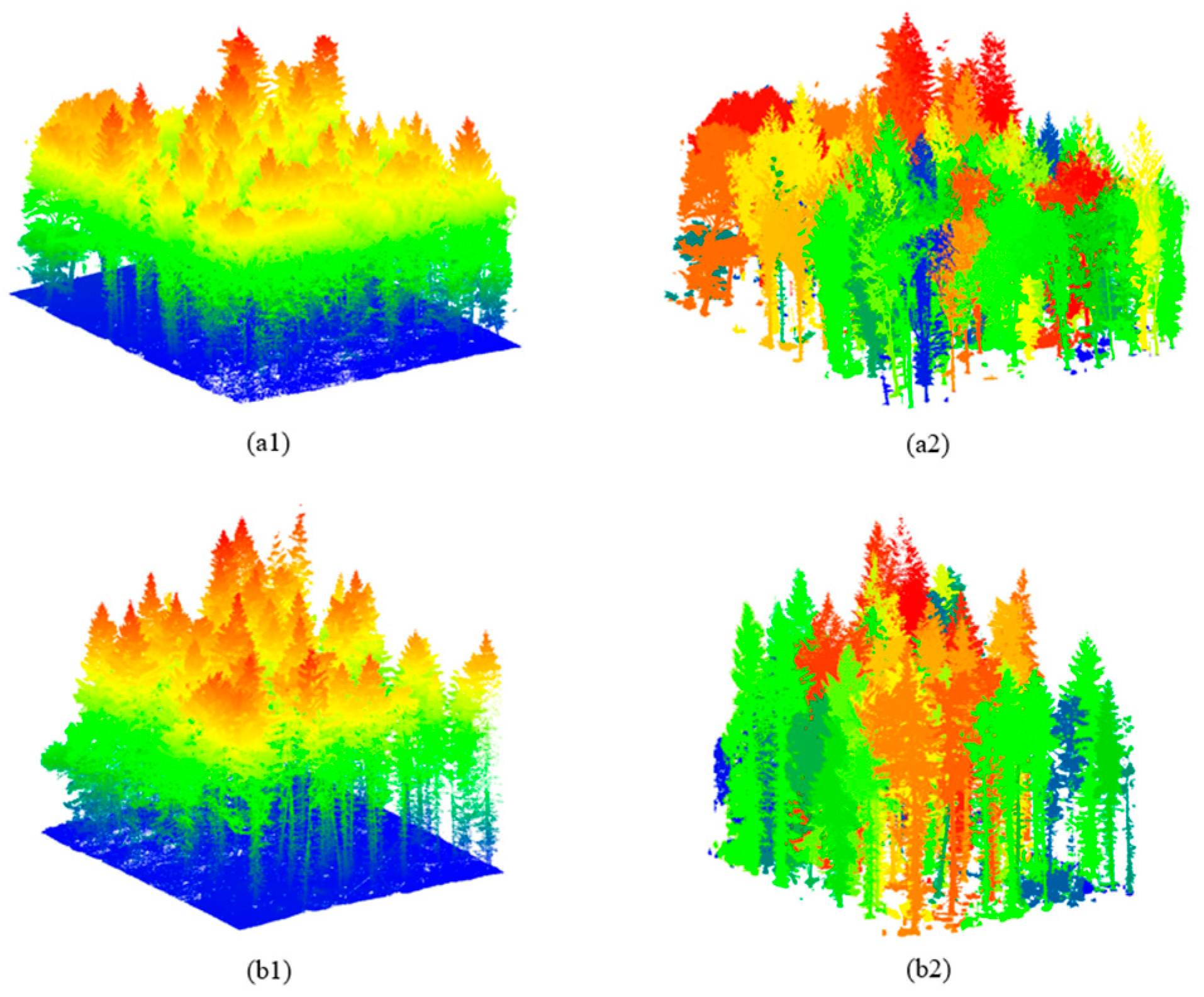
To examine the effectiveness of the proposed method for a real dataset, an openly available dataset was included in this study. The dataset was obtained from the 2017 Speulderbos laser-scanning campaign and covered approximately 2 ha of forest [43]. An approximately 50 × 50 plot and an approximately 30 × 30 plot were clipped from the UAV–LiDAR dataset. To acquire accurate referenced individual-tree characteristics, the single-tree isolation MATLAB tool was applied to corresponding TLS point clouds [44], and a manual correction for some wrong segmentation was then adopted in CloudCompare. Figure 2 shows these two plots and the individual-tree segmentation result of the TLS point clouds.

2.2. Methodology

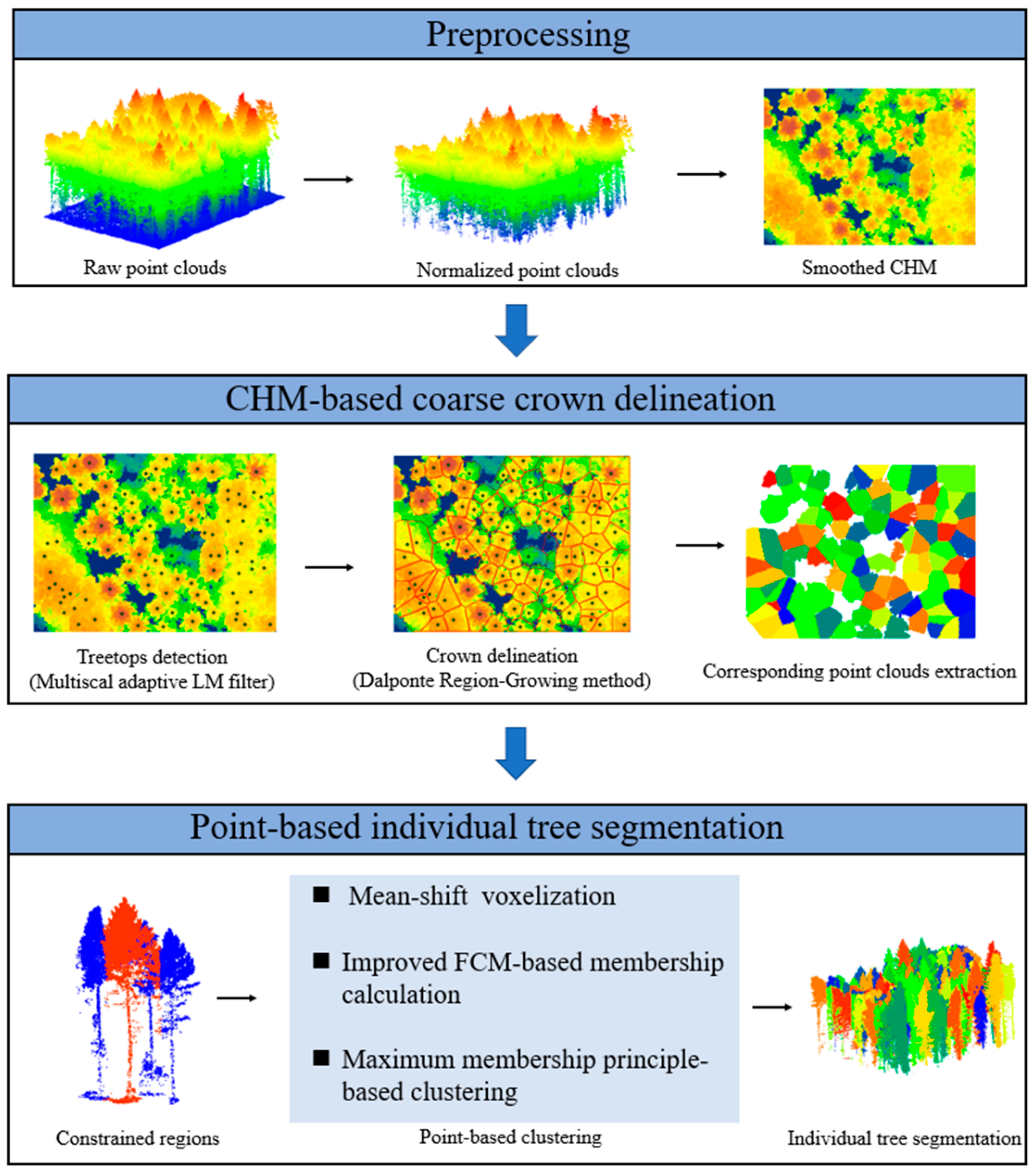
In this study, a novel algorithm was devised for segmenting individual trees. Specifically, coarse crowns were first segmented on a CHM with the use of a multiscale adaptive LM filter to identify treetops and an RG method to obtain crowns. Point clouds extracted from a coarse crown and its neighbors were transformed into supervoxels via a mean-shift voxelization method. Then, the supervoxels were clustered based on the maximum membership degree principle. Figure 3 shows the workflow of the proposed method, which comprised three main parts: preprocessing, CHM-based coarse-crown delineation, and point-based individual-tree segmentation.

2.2.1. Preprocessing

For actual UAV–LiDAR data, a statistical outlier filter (SOR) was applied to remove noise and outliers. Next, the remaining points were classified into ground points and nonground points with the use of cloth simulation filtering [45]. For the cloth simulation filter, the cloth resolution was 0.2, and the max iterations and classification threshold were both default values. Then, ground points were used to create the digital elevation model, and normalized point clouds were obtained by subtracting the value of the corresponding DSM raster from the elevation of the nonground points.
Then, a CHM with a 0.2 m pixel size was derived from the normalized point clouds. Because the simulated dataset was generated using individual-tree point clouds that had been normalized, the CHM could be directly obtained via rasterization without the above processes.
Because the noise in a CHM might affect the detection of the LM, a smooth filter was used to smooth the CHM. The typical filters adopted in previous studies were median and Gaussian filters. However, some fine shape features important in crown delineation might have been missing if those filters had been used. In this study, an adaptive Gaussian filter was applied to the CHM, which could adaptively suppress the noise and preserve sharp features.

2.2.2. Treetop Detection

An LM filter is the most common method to identify individual trees [15,18]. It is based on the assumption that treetops are the local highest values in a CHM. LM filters can be classified into fixed- and variable-window filters. Variable windows are more appropriate than fixed ones because a region’s crown sizes vary. Usually, it is assumed that crown sizes strongly relate to tree heights, and a linear or nonlinear regression model is adopted to predict window sizes in filtering [46,47]. However, a linear regression might not be appropriate in all the plots. Moreover, crown sizes not only depend on the tree height but also are associated with the tree species. For example, broadleaved trees’ crown sizes are larger than those of coniferous trees. Thus, another indicator must be selected that can accurately reflect the crown size.
Therefore, a multiscale adaptive LM filter based on a GLCM was designed in this study to locate individual trees. It was assumed that the values of the CHM are similar for large crowns and that the values of the CHM for small crowns have a higher degree of heterogeneity. Then, an angular second moment (ASM) could be adopted to measure the uniformity of the height values within crowns.
The smoothed CHM was transformed into an n-bit grayscale image via Jenks natural breaks optimization [48]. A GLCM and an ASM were generated in filter windows of various sizes passing over the smoothed CHM. Specifically, the ASM was divided by the number of pixels, n, in the filter window to mitigate the effects of the window size. Equation (1) shows the calculation of n_ASM, where p ( i , j ) is the ( i , j ) th value in the GLCM, and N is the total number of pixels in the filter window as follows:
n_ASM = i j p ( i , j ) 2 N
For each pixel, the window size corresponding to the max n_ASM was adopted as the size of the LM filter. Figure 4 is a flowchart of the adaptive LM filter. A multiscale filter was used to search for the proper window size for each crown.
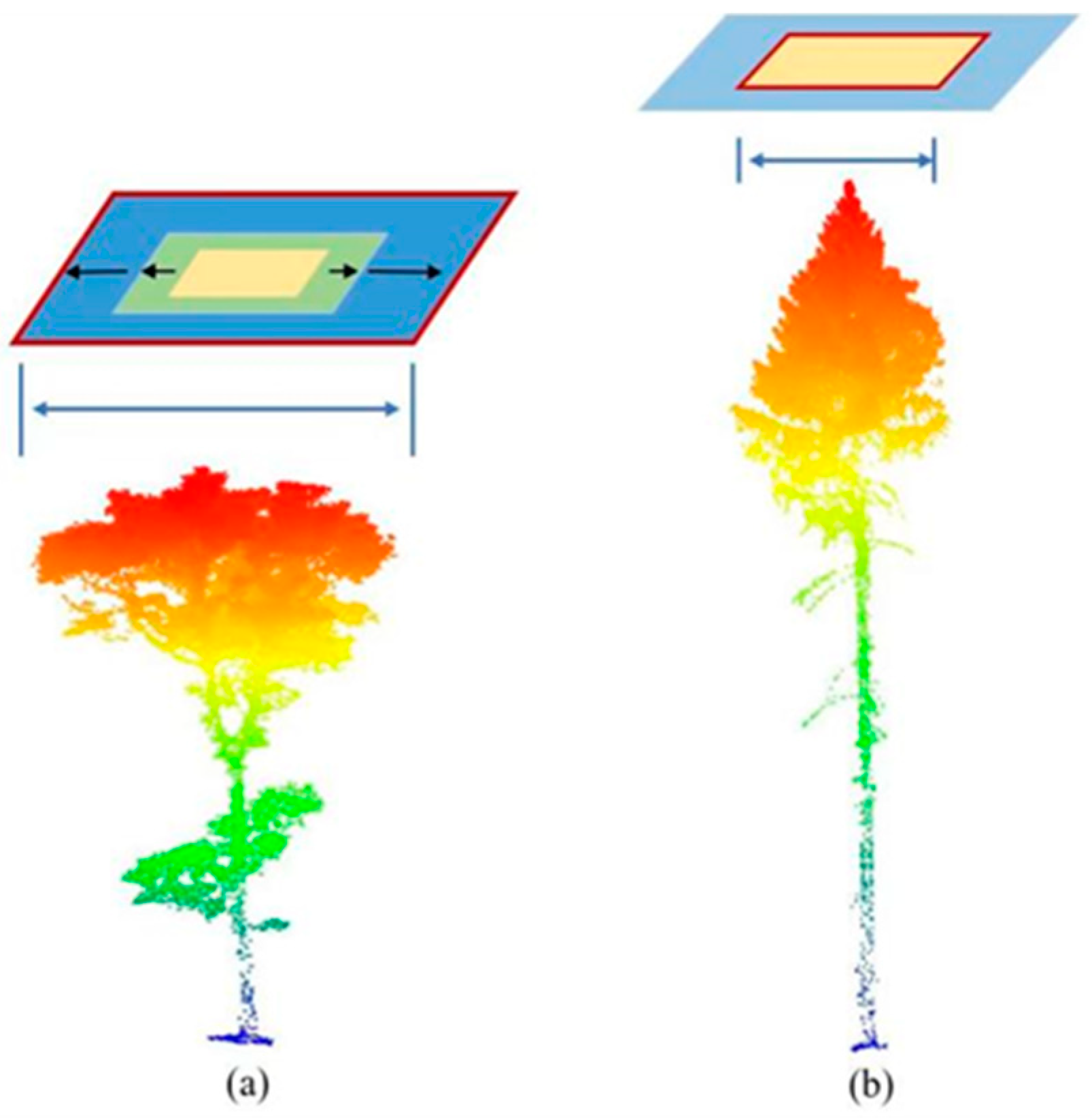
Figure 5 shows the central concept of the adaptive LM filter algorithm. For coniferous trees, n_ASM would reach the maximum at a small window size (Figure 5b), whereas for broadleaved trees, the max n_ASM would be obtained with a larger window because the canopy edge would be included, which could contribute to the value of the ASM (Figure 5a).

2.2.3. CHM-Based Crown Delineation

After the treetop detection, a seeded RG method was used for the coarse-crown segmentation [24]. The algorithm took each maximum as the initial seed and then neighboring pixels were added to the crown region by considering a series of criteria: (1) the neighboring pixel heights exceeded the seed height × σ1 and the mean height of the current crown × σ2, (2) the neighboring pixel heights were below the seed height × σ3, and (3) the maximum distance between the growing pixels and the seed was σ4. These threshold values were set based on the current tree information. Additionally, σ1 and σ2 were decimals between 0 and 1, σ3 was a decimal greater than 1, and σ4 should be similar to the crown radius. The constrained regions were extracted based on the coarse crowns in the further point-based segmentation.

2.2.4. Point-Based Individual-Tree Segmentation

The contours of the tree crowns derived from the CHM-based method were prone to inaccuracy due to the loss of 3D information. Especially in high-density forests, where crowns are often clumped and overlapped, the common problem is that the small trees would be under-segmented. Therefore, point-based methods, which directly segment individual trees in 3D space, were used to adjust the result of the coarse-crown segmentation.
Normally, clustering methods assign each point to only one cluster, but in forests, the boundaries between adjacent crowns are blurred, and traditional clustering methods might fail to alleviate the ambiguity. To address the clustering uncertainty of point clouds at crown boundaries, a weighted FCM method was used to calculate the degree of membership of each supervoxel. These supervoxels were then assigned to corresponding clusters based on the maximum membership degree principle. Figure 6 shows the detailed workflow for the fine segmentation. Notably, the traversal of the trees was in descending order by the height.
  • Constrained region extraction: First, a zone method was used because of the computational complexity for large-scale point clouds. This method also eliminated the effect of the distance on the clustering because the tree-crown sizes varied, and the tree distributions were uneven, which would restrict the distance-based cluster methods. Other hybrid methods defined each coarse crown derived from the CHM as a constrained region, and point-based treetop reidentification and clustering were conducted in such regions. However, these methods worked only when there was under-segmentation of subdominant trees because they did not consider the neighboring region. In this study, new constrained regions were defined with the use of a neighbor-searching method. For each tree, the constrained region comprised its k-nearest neighbor crowns and itself, and a distance threshold was applied to remove the far-neighbor crowns. Then, the point clouds in constrained regions were extracted, and further clustering was conducted in the region;
  • Mean-shift voxelization: A mean-shift voxelization method was applied to obtain supervoxels. Relative to traditional voxel-based methods, which transform point clouds into cubic voxels at a fixed resolution, mean-shift voxelization is more robust and flexible [30] and groups points by iteratively shifting each point to the density maxima via a kernel. Considering the various point cloud densities in different constrained regions, a bandwidth estimation technique was used to choose the appropriate bandwidth for each region;
  • Maximum membership degree principle-based supervoxel clustering: Given the boundary’s ambiguity, for each coarse single-tree point cloud and its neighbors, an FCM was adopted to complete the fine segmentation [49]. Fuzzy c-means is a data-clustering technique where each data point belongs to a cluster to a degree that is specified by a membership grade. Because the supervoxels aggregated different quantities of points, in this study, a sample weight for each supervoxel was introduced to the objective function of the FCM (Equation (2)).
    J = i = 1 C j = 1 N μ i j m n j x j v i 2
    where μ i j m is the membership of the supervoxel, x j , and for each supervoxel, the membership in all the clusters adds to 1. N is the number of supervoxels in a constrained region, C is the number of clusters, m is a weighting exponent, v i is the centroid of cluster i , n j is a weight for the number of points in each supervoxel, and x j v i 2 is the Euclidian distance between x j and v i . The optimization problem of J could be solved with the use of a Lagrange multiplier (Equation (3)). Then, by calculating the first derivatives of u i j and v i for the constraint function L u i j , v i , λ j and setting them equal to zero, two optimal parameters were obtained (Equations (4) and (5), respectively). After an iterative process, the objective function, J, was minimized until the centroid distance was less than a low threshold.
    L u i j , v i , λ j = i = 1 C j = 1 N μ i j m n j x j v i 2 j = 1 N λ j i = 1 C μ i j 1
    μ i j = 1 x j v i 2 m 1 i = 1 C 1 x j v i 2 m 1
    v i = j = 1 N n j μ i j m x j j = 1 N n j μ i j m
Specifically, the number of clusters, C , was the total number of treetops in a constrained region, and the initialization of μ i j m relied on the locations of the treetops, which were defined as the initial centroids.
After clustering, each supervoxel was assigned a membership vector and then each point in the supervoxels was labeled based on the maximum membership principle. Because the clustering labels were meaningless, the new label of the original tree was still unknown. To determine the corresponding tree label, an intersection method was considered. It counted the number of point clouds where the original target tree intersected with each new tree cluster. The new target tree was the cluster that had the maximum number of intersections.
Also, the points in a new individual tree might have been classified in the last fine segmentation. Based on that condition, the memberships of the two points were compared, and the point with the highest membership was labeled as the class.

2.2.5. Accuracy Assessment

To evaluate the effect of the multiscale adaptive LM filter, a temporary coarseness-matching method was adopted. It was assumed that the two treetops were matched if the horizontal distances between the detected treetops and true treetops were below half the plot’s average tree-crown width. The detection results were evaluated using three indicators: the tree detection rate, r (recall); the correctness of the detected trees, p (precision); and the overall accuracy of the detected trees, f, (Equations (6)–(8), respectively) as follows:
r = T P / ( T P + F N )
p = T P / ( T P + F P )
f = 2 × ( r × p ) / ( r + p )
Many studies use tree-to-tree match-pairing agreements to assess the accuracy of the individual-tree segmentation. Such methods select simple linear-distance thresholds to match detected trees with reference trees. However, these measures fail to represent the multivariate nature of individual-tree segmentations and would lead to a misleading assessment.
Therefore, an ARBOR method was used in this study to quantify the agreement between the reference tree datasets and detected trees. The framework was proposed by Murray et al. [41] and models trees as Gaussian curves with the use of biophysical properties (tree location, tree height, and crown area). A Jaccard similarity coefficient was then developed to assess the agreements of the trees in different datasets as follows:
J A , B = A B / ( A + B A B )
A Hungarian combinatorial optimization algorithm was applied to achieve match pairing based on the Jaccard similarity coefficient. Finally, two metrics were calculated, the average match-pairing similarity (AMPS) index and the dataset size similarity (DSS) index. As shown in Equations (10) and (11), the AMPS index assesses the overall quality of the matched pairs, and the DSS index indicates similar tree population sizes in two datasets, respectively.
A M P S = i = 1 m J A , B / m
D S S = m / ( a + b m )
where m is the number of paired trees, and a and b are the numbers of trees in datasets A and B, respectively. Notably, unlike the ARBOR framework, in this study, not all pairs matched using the Hungarian algorithm were used to calculate the above two indicators. Imperfect pairs were defined by a Jaccard similarity coefficient of matched pairs below a threshold and were abandoned.
Also, following the matching procedure, the accuracies of the estimated tree-crown areas and tree heights were evaluated using linear regression. The R-squared values of the reference metrics and UAV–LiDAR-derived metrics were also calculated.

3. Results

3.1. Treetop Detection

Figure 7 shows two examples of treetop detection. The top row shows plots of coniferous trees, and the bottom row shows broadleaved plots. Figure 7(a1,a2) show the treetop detection result obtained with the use of the multiscale adaptive LM filter proposed in this study. A traditional LM method was also applied to those two plots as a comparison. Two fixed window sizes were chosen. The results are displayed in Figure 2(b2) and Figure 7(b1,c1,c2). As shown in Figure 7 most of the treetops were detected in the two plots. The red boxes highlight the main differences between these two methods. The LM filter with the larger window tended to omit true treetops, and that with the smaller window had more commission errors. The method proposed in this study had better detection that achieved a balance between omission and commission. Also, the distances between the true treetops and detected treetops in the broadleaved trees were longer than those between the true treetops and detected treetops in the coniferous trees. That was because broadleaved trees usually have larger crowns and flatter inner foliage than coniferous trees.
Table 2 shows the average rates of treetop detection in all the plots. Although the LM with the larger window had higher p values and the LM with the smaller window had higher r values, the adaptive LM based on the GLCM had a higher overall accuracy. The higher treetop detection rate of the LM with the smaller window was at the expense of more false-detected treetops. The LM with the larger window had a higher p value but at the expense of the treetop detection rate.

3.2. Individual-Tree Segmentation

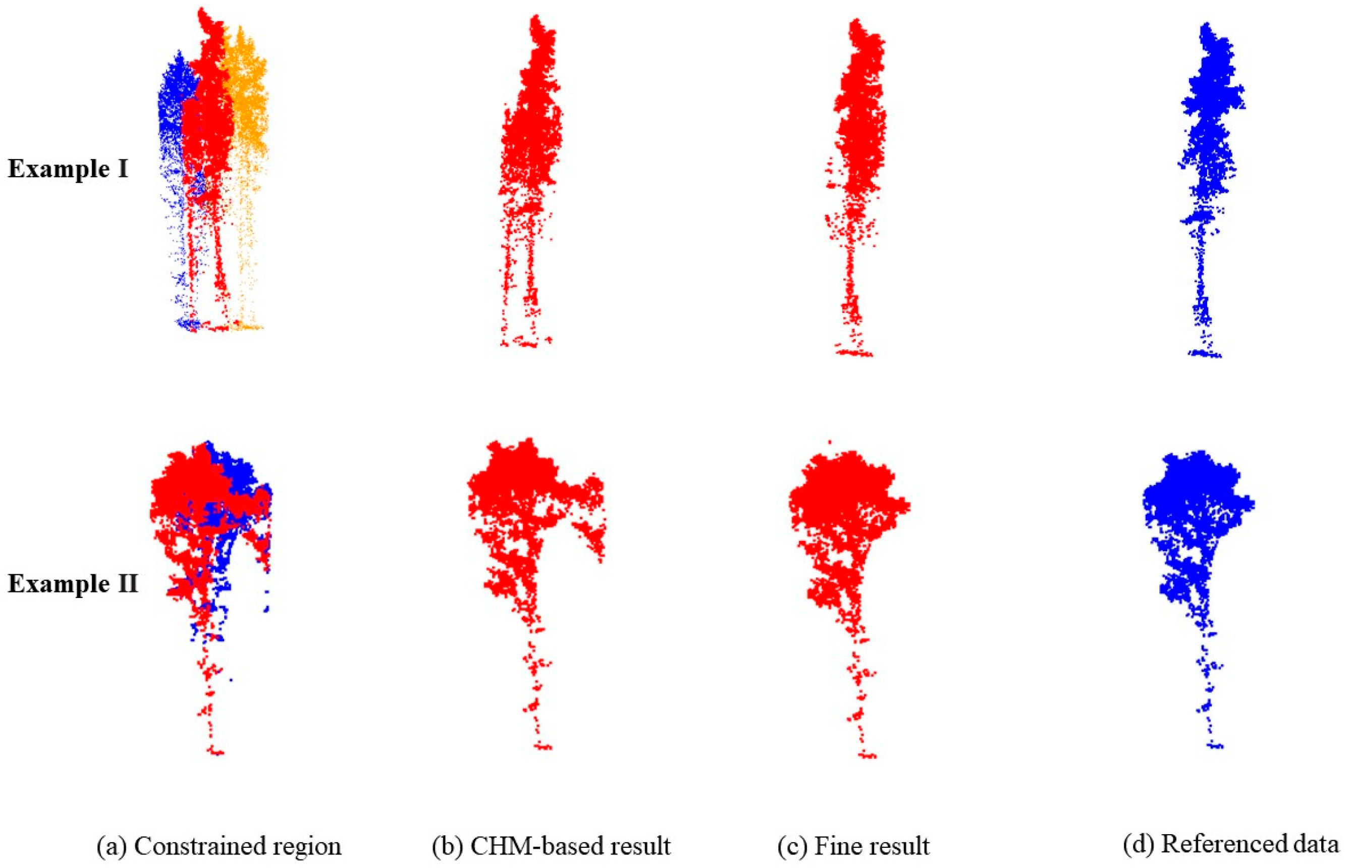
The individual-tree point cloud extracted using the CHM-based method was coarse because it only considered the canopy height information. Figure 8 shows two examples of the individual-tree point clouds derived from CHM-based crowns and other point-based clustering results. In Example I, according to the 2D-segmented result, the smaller tree’s point cloud was classified as a part of the target individual-tree clouds. The under-segmented part was abandoned in the point-based clustering process, which used 3D spatial information. In Example II, because the heights of the trees were similar, partially neighboring crowns’ point clouds were assigned to the target tree, and the crown’s inner foliage missed some points. This clustering method filled the empty areas and cut the excess points by re-segmenting in the neighboring constrained region.
Figure 9 shows four example plots of segmentation results, suggesting that the method proposed in this study performed well in individual-tree segmentation.

3.3. Results for the Accuracy of the Remotely Sensed Biophysical Observation and Retrieval (ARBOR) Framework

The accuracy of the individual-tree segmentation was assessed in the ARBOR framework, as mentioned above. AMPS and DSS were calculated for different plots. A high AMPS meant a better overall match for the paired trees, and a high DSS meant a greater degree of similarity between the tree population sizes. Different from the simple treetop-matching method described in Section 3.1, ARBOR achieved match pairing in accordance with the Jaccard similarity coefficient. As described in previous sections, the Jaccard similarity coefficient considered the tree location, height, and crown area. Thus, relative to the matching method based on treetop horizontal distances, DSS and AMPS were stricter indicators of the individual-tree identification and segmentation.
All the synthetic plots were divided into five classes and then the means of the AMPS and DSS were obtained in various classes. The results are shown in Table 3.
The low-density coniferous plots achieved the highest AMPS and DSS, at 0.8237 and 0.7547, respectively. The high-density broadleaved forests had the lowest AMPS, and the mixed forest had the lowest DSS. Generally, the accuracy of the coniferous plots was higher than those of the broadleaved and mixed plots. That was because coniferous treetops could be detected more easily using the LM filter method, and the crowns of broadleaved trees were more complex than those of coniferous trees, which made individual-tree segmentation more difficult. Also, the segmentation results were influenced by the plots’ densities. Trees in higher-density plots were prone to clumping and overlapping, often leading to treetop detection errors and the under- or over-segmentation of tree crowns. Owing to the complexity of the tree species, AMPS and DSS were low for the mixed plots.
For two actual LiDAR plots, the AMPS and DSS of plot1 were 0.6469 and 0.6449, respectively, and the AMPS and DSS of plot2 were 0.7080 and 0.6667, respectively, which indicated that the proposed method also worked well for actual LiDAR datasets.
Furthermore, the accuracy of the tree heights and crown areas was evaluated. The correlation between the reference metrics and UAV–LiDAR-derived metrics was analyzed. The results are shown in Figure 10. The tree-height and crown-area metrics both showed good agreement, with R2 values of 0.8391 and 0.6404, respectively. Indeed, the tree height showed a stronger correlation than the crown area because the estimation of the crown-area metric was more complex and tended to be affected by other factors, such as the definition and measurement methods of the crown area. In this study, the horizontal projection of individual-tree point clouds was first obtained, and the convex hull area was taken as the crown area, which was a rough estimation.

3.4. Comparison with Existing Methods

The proposed method was compared with other existing methods, including the point-based method proposed by Li in 2012, the RG method proposed by Dalponte in 2016, and the classic watershed algorithm [24,32]. The method proposed by Li was implemented in lidR [50], and the Dalponte method and the classic watershed algorithm were implemented in Python. Table 3 summarizes the AMPS and DSS of the various methods. The results show that the two indicators of the proposed method in this study were generally higher than those of the other methods. Additionally, it was found that the AMPS of the mixed plots and real plot1 were higher than that of our method; that could be explained by the number of matched pairs. According to the definition of AMPS in the ARBOR framework, AMPS is the mean Jaccard similarity coefficient of the matched pairs. Therefore, AMPS not only depends on the agreement of each pair but also is influenced by the number of matched pairs, which could be measured using DSS. As shown in Table 3, the DSS values of the other methods were lower than those of the proposed method; thus, the other methods had fewer matched pairs, which might have contributed to the higher AMPS. Additionally, owing to the zonalization and supervoxelization of the point clouds, the computational performance of the proposed method was also better than those of other point-based algorithms [3]. The runtime of our method was approximately 530 s for one 30 × 30 m plot at ~600 pt/m2.
Table 3. Comparison of segmentation accuracies obtained in the ARBOR framework.
PlotMethod
Proposed MethodLi 2012DalponteWatershed
AMPSDSSAMPSDSSAMPSDSSAMPSDSS
Coniferous plots (L)0.82370.75470.80540.72450.78240.70440.79400.7213
Coniferous plots (H)0.74980.66790.67750.49050.65360.53220.59430.6626
Broadleaved plots (L)0.70330.55420.66260.48750.68440.48730.67970.4417
Broadleaved
plots (H)
0.63990.60730.61320.54700.55300.58140.59260.5458
Mixed plots0.66030.52940.69360.50130.65460.48640.67000.4345
Real plot10.64690.64490.65120.52730.62230.61700.67110.5857
Real plot20.70800.66670.70240.43660.69350.59700.69870.5735

4. Discussion

4.1. Parameter Analysis

The performance of the proposed method depended on the parameter values. Two key parameters accounted for the accuracy of the individual-tree segmentation. First, the moving window size of the LM filter was important for the treetop detection accuracy. The window size, S, relied on the crowns’ sizes in the plots. According to the tests on different plots in this study, higher Smin and Smax values are advisable for plots with larger crowns and vice versa. In our studies, for broadleaved plots, Smax was approximately 10, and Smin was approximately 6 (in pixels, radius). For coniferous plots, Smax was approximately 6, and Smin was approximately 3. The stem density of the plots also affected the results of the treetop detection. Most studies have focused on the relation between tree-crowns and other metrics, such as tree heights, and are based on individual trees. That relation would not be suitable in high-density plots where trees are clumped and crowns overlap. For high-density plots, because the distances between trees are shorter, the window size threshold should be set lower. Therefore, the values of Smin and Smax should be further adjusted for the tree density in plots.
Additionally, the bandwidth used in the mean-shift voxelization is important. Because the number of points in different constrained regions varies, the bandwidth function estimated with the use of percentiles in Python’s Scikit-learn library was adopted to select suitable bandwidths for different regions. In accordance with previous studies and our own experiments, the quantile parameter was set at the ratio of the point density to the number of points in constrained regions. Notably, when the point density was high, a coefficient k (from 0 to 1) was introduced to improve the computational efficiency. Indeed, the quantile value affected the algorithm’s computational efficiency from two aspects: (1) a higher quantile increased the computational time of the bandwidth estimation function, and (2) a lower quantile led to more supervoxels. Therefore, more pair distances were calculated during the process of the membership initialization. Specifically, for better clustering performance, the Z values of all the point clouds were divided by six before the fine segmentation.

4.2. Synthetic Dataset Compared with Actual LiDAR Dataset

In this study, a synthetic dataset was generated and used to test the performance of the proposed method. Indeed, simulated forest data have been adopted in studies related to individual-tree segmentation problems. Liu et al. [23] created a simulated forest to test an individual-tree identification algorithm. They first generated random tree locations, and then 3D point clouds were created based on specific functions. Wang et al. [35] also explored an unsupervised semantic and instance segmentation algorithm based on a synthetic dataset, which was modeled using SpeedTree software (Interactive Data Visualization, Inc., Lexington, SC, USA) and simulated using HELIOS.
Synthetic datasets are available at lower costs than actual LiDAR datasets. Thus, diverse forest conditions can be simulated to test algorithm robustness and better understand the relation between plot characteristics and algorithm parameters. Also, the synthetic datasets bypassed some problems in the actual LiDAR data [51,52,53]. The ground reference data also excluded measurement errors, such as tree trunk location deviations.
However, in actual LiDAR datasets, some problems exist that are not present in synthetic datasets. For example, individual-tree segmentation results are substantially affected by surface topography [54,55]. In steep areas, the normalization of the point cloud may change the shape of crowns and would affect the performance of the proposed algorithms. It is suggested that the terrain’s slope be considered when simulating a forest LiDAR dataset. Future works should focus on the robustness of the proposed method, considering various terrains.

5. Conclusions

Individual-tree segmentation for UAV–LiDAR data remains challenging owing to the increased number of points. In this study, to better extract single-tree point clouds, a hybrid method was devised by combining the CHM-based method and the point-based method. First, a multiscale adaptive LM filter based on GLCM was used to detect treetops accurately, and a Dalponte RG method was introduced to achieve crown delineation. Based on coarse crowns, a neighboring constrained region was extracted for each tree. Then, a mean-shift voxelization was conducted in the region, and a supervoxel-weighted FCM initialized by treetops was used to calculate memberships.
Finally, new individual trees were segmented based on the maximum membership principle. The algorithm was tested on a simulated dataset and an actual LiDAR dataset and evaluated using the ARBOR framework; that framework considered not only tree locations but also tree heights and crown areas. The results showed that the proposed method performed better than existing methods. Accurate individual-tree segmentation can provide detailed forest information and contribute to more precise forestry management and carbon stock estimation at an individual-tree scale.

Author Contributions

Conceptualization, Y.F. and Y.N.; methodology, Y.F.; validation, Y.F.; formal analysis, Y.F.; resources, Y.N.; writing—original draft preparation, Y.F.; writing—review and editing, Y.F., Y.N., L.W. and W.L.; visualization, Y.F.; supervision, Y.N.; project administration, Y.N., L.W. and W.L.; funding acquisition, L.W. All authors have read and agreed to the published version of the manuscript.

Funding

This research was funded by the National Key Research and Development Project of China (grant 2021YFB3901305), the National Natural Science Foundation of China (grants U2244230 and 42171369), the Youth Innovation Promotion Association of the Chinese Academy of Sciences (grant Y2022051), and the Director Fund of the International Research Center of Big Data for Sustainable Development Goals (grant CBAS2022DF012).

Data Availability Statement

The employed UAV–LiDAR dataset is derived from a publicly available database https://doi.pangaea.de/10.1594/PANGAEA.942856 (accessed on 31 March 2022).

Conflicts of Interest

The authors declare no conflicts of interest.

References

  1. Li, W.; Guo, W.-Y.; Pasgaard, M.; Niu, Z.; Wang, L.; Chen, F.; Qin, Y.; Svenning, J.-C. Human Fingerprint on Structural Density of Forests Globally. Nat. Sustain. 2023, 6, 368–379. [Google Scholar] [CrossRef]
  2. Pan, Y.; Birdsey, R.A.; Fang, J.; Houghton, R.; Kauppi, P.E.; Kurz, W.A.; Phillips, O.L.; Shvidenko, A.; Lewis, S.L.; Canadell, J.G.; et al. A Large and Persistent Carbon Sink in the World’s Forests. Science 2011, 333, 988–993. [Google Scholar] [CrossRef]
  3. Hao, Y.; Widagdo, F.R.A.; Liu, X.; Liu, Y.; Dong, L.; Li, F. A Hierarchical Region-Merging Algorithm for 3-d Segmentation of Individual Trees Using UAV-LiDAR Point Clouds. IEEE Trans. Geosci. Remote Sens. 2021, 60, 5701416. [Google Scholar] [CrossRef]
  4. Liang, X.; Wang, Y.; Pyörälä, J.; Lehtomäki, M.; Yu, X.; Kaartinen, H.; Kukko, A.; Honkavaara, E.; Issaoui, A.E.; Nevalainen, O.; et al. Forest in Situ Observations Using Unmanned Aerial Vehicle as an Alternative of Terrestrial Measurements. For. Ecosyst. 2019, 6, 20. [Google Scholar] [CrossRef]
  5. Bai, J.; Niu, Z.; Gao, S.; Bi, K.; Wang, J.; Huang, Y.; Sun, G. An Exploration, Analysis, and Correction of the Distance Effect on Terrestrial Hyperspectral LiDAR Data. ISPRS J. Photogramm. Remote Sens. 2023, 198, 60–83. [Google Scholar] [CrossRef]
  6. Kotivuori, E.; Kukkonen, M.; Mehtätalo, L.; Maltamo, M.; Korhonen, L.; Packalen, P. Forest Inventories for Small Areas Using Drone Imagery without In-Situ Field Measurements. Remote Sens. Environ. 2020, 237, 111404. [Google Scholar] [CrossRef]
  7. Li, W.; Niu, Z.; Shang, R.; Qin, Y.; Wang, L.; Chen, H. High-Resolution Mapping of Forest Canopy Height Using Machine Learning by Coupling ICESat-2 LiDAR with Sentinel-1, Sentinel-2 and Landsat-8 Data. Int. J. Appl. Earth Obs. Geoinf. 2020, 92, 102163. [Google Scholar] [CrossRef]
  8. Wang, Y.; Lehtomäki, M.; Liang, X.; Pyörälä, J.; Kukko, A.; Jaakkola, A.; Liu, J.; Feng, Z.; Chen, R.; Hyyppä, J. Is Field-Measured Tree Height as Reliable as Believed–A Comparison Study of Tree Height Estimates from Field Measurement, Airborne Laser Scanning and Terrestrial Laser Scanning in a Boreal Forest. ISPRS J. Photogramm. Remote Sens. 2019, 147, 132–145. [Google Scholar] [CrossRef]
  9. Zhen, Z.; Yang, L.; Ma, Y.; Wei, Q.; Jin, H.I.; Zhao, Y. Upscaling Aboveground Biomass of Larch (Larix Olgensis Henry) Plantations from Field to Satellite Measurements: A Comparison of Individual Tree-Based and Area-Based Approaches. GIScience Remote Sens. 2022, 59, 722–743. [Google Scholar] [CrossRef]
  10. Du, L.; Pang, Y.; Wang, Q.; Huang, C.; Bai, Y.; Chen, D.; Lu, W.; Kong, D. A LiDAR Biomass Index-Based Approach for Tree-and Plot-Level Biomass Mapping over Forest Farms Using 3D Point Clouds. Remote Sens. Environ. 2023, 290, 113543. [Google Scholar] [CrossRef]
  11. Brede, B.; Terryn, L.; Barbier, N.; Bartholomeus, H.M.; Bartolo, R.; Calders, K.; Derroire, G.; Moorthy, S.M.K.; Lau, A.; Levick, S.R.; et al. Non-Destructive Estimation of Individual Tree Biomass: Allometric Models, Terrestrial and UAV Laser Scanning. Remote Sens. Environ. 2022, 280, 113180. [Google Scholar] [CrossRef]
  12. Mielcarek, M.; Stereńczak, K.; Khosravipour, A. Testing and Evaluating Different LiDAR-Derived Canopy Height Model Generation Methods for Tree Height Estimation. Int. J. Appl. Earth Obs. Geoinf. 2018, 71, 132–143. [Google Scholar] [CrossRef]
  13. Vega, C.; Hamrouni, A.; El Mokhtari, S.; Morel, J.; Bock, J.; Renaud, J.-P.; Bouvier, M.; Durrieu, S. PTrees: A Point-Based Approach to Forest Tree Extraction from Lidar Data. Int. J. Appl. Earth Obs. Geoinf. 2014, 33, 98–108. [Google Scholar] [CrossRef]
  14. Wu, B.; Yu, B.; Wu, Q.; Huang, Y.; Chen, Z.; Wu, J. Individual Tree Crown Delineation Using Localized Contour Tree Method and Airborne LiDAR Data in Coniferous Forests. Int. J. Appl. Earth Obs. Geoinf. 2016, 52, 82–94. [Google Scholar] [CrossRef]
  15. Dralle, K.; Rudemo, M. Stem Number Estimation by Kernel Smoothing of Aerial Photos. Can. J. For. Res. 1996, 26, 1228–1236. [Google Scholar] [CrossRef]
  16. Koch, B.; Heyder, U.; Weinacker, H. Detection of Individual Tree Crowns in Airborne Lidar Data. Photogramm. Eng. Remote Sens. 2006, 72, 357–363. [Google Scholar] [CrossRef]
  17. Wulder, M.; Niemann, K.O.; Goodenough, D.G. Local Maximum Filtering for the Extraction of Tree Locations and Basal Area from High Spatial Resolution Imagery. Remote Sens. Environ. 2000, 73, 103–114. [Google Scholar] [CrossRef]
  18. Popescu, S.C.; Wynne, R.H.; Nelson, R.F. Estimating Plot-Level Tree Heights with Lidar: Local Filtering with a Canopy-Height Based Variable Window Size. Comput. Electron. Agric. 2002, 37, 71–95. [Google Scholar] [CrossRef]
  19. Yin, D.; Wang, L. Individual Mangrove Tree Measurement Using UAV-Based LiDAR Data: Possibilities and Challenges. Remote Sens. Environ. 2019, 223, 34–49. [Google Scholar] [CrossRef]
  20. Falkowski, M.J.; Smith, A.M.; Hudak, A.T.; Gessler, P.E.; Vierling, L.A.; Crookston, N.L. Automated Estimation of Individual Conifer Tree Height and Crown Diameter via Two-Dimensional Spatial Wavelet Analysis of Lidar Data. Can. J. Remote Sens. 2006, 32, 153–161. [Google Scholar] [CrossRef]
  21. Barnes, C.; Balzter, H.; Barrett, K.; Eddy, J.; Milner, S.; Suárez, J.C. Individual Tree Crown Delineation from Airborne Laser Scanning for Diseased Larch Forest Stands. Remote Sens. 2017, 9, 231. [Google Scholar] [CrossRef]
  22. Persson, A.; Holmgren, J.; Soderman, U. Detecting and Measuring Individual Trees Using an Airborne Laser Scanner. Photogramm. Eng. Remote Sens. 2002, 68, 925–932. [Google Scholar]
  23. Liu, H.; Dong, P.; Wu, C.; Wang, P.; Fang, M. Individual Tree Identification Using a New Cluster-Based Approach with Discrete-Return Airborne LiDAR Data. Remote Sens. Environ. 2021, 258, 112382. [Google Scholar] [CrossRef]
  24. Dalponte, M.; Coomes, D.A. Tree-Centric Mapping of Forest Carbon Density from Airborne Laser Scanning and Hyperspectral Data. Methods Ecol. Evol. 2016, 7, 1236–1245. [Google Scholar] [CrossRef] [PubMed]
  25. Duncanson, L.; Cook, B.; Hurtt, G.; Dubayah, R. An Efficient, Multi-Layered Crown Delineation Algorithm for Mapping Individual Tree Structure across Multiple Ecosystems. Remote Sens. Environ. 2014, 154, 378–386. [Google Scholar] [CrossRef]
  26. Liu, T.; Im, J.; Quackenbush, L.J. A Novel Transferable Individual Tree Crown Delineation Model Based on Fishing Net Dragging and Boundary Classification. ISPRS J. Photogramm. Remote Sens. 2015, 110, 34–47. [Google Scholar] [CrossRef]
  27. Yun, T.; Jiang, K.; Li, G.; Eichhorn, M.P.; Fan, J.; Liu, F.; Chen, B.; An, F.; Cao, L. Individual Tree Crown Segmentation from Airborne LiDAR Data Using a Novel Gaussian Filter and Energy Function Minimization-Based Approach. Remote Sens. Environ. 2021, 256, 112307. [Google Scholar] [CrossRef]
  28. Pang, Y.; Wang, W.; Du, L.; Zhang, Z.; Liang, X.; Li, Y.; Wang, Z. Nyström-Based Spectral Clustering Using Airborne LiDAR Point Cloud Data for Individual Tree Segmentation. Int. J. Digit. Earth 2021, 14, 1452–1476. [Google Scholar] [CrossRef]
  29. Morsdorf, F.; Meier, E.; Allgöwer, B.; Nüesch, D. Clustering in Airborne Laser Scanning Raw Data for Segmentation of Single Trees. Int. Arch. Photogramm. Remote Sens. Spat. Inf. Sci. 2003, 34, W13. [Google Scholar]
  30. Ferraz, A.; Saatchi, S.; Mallet, C.; Meyer, V. Lidar Detection of Individual Tree Size in Tropical Forests. Remote Sens. Environ. 2016, 183, 318–333. [Google Scholar] [CrossRef]
  31. du Toit, F.; Coops, N.C.; Ratcliffe, B.; El-Kassaby, Y.A.; Lucieer, A. Modelling Internal Tree Attributes for Breeding Applications in Douglas-Fir Progeny Trials Using RPAS-ALS. Sci. Remote Sens. 2023, 7, 100072. [Google Scholar] [CrossRef]
  32. Li, W.; Guo, Q.; Jakubowski, M.K.; Kelly, M. A New Method for Segmenting Individual Trees from the Lidar Point Cloud. Photogramm. Eng. Remote Sens. 2012, 78, 75–84. [Google Scholar] [CrossRef]
  33. Sačkov, I.; Hlásny, T.; Bucha, T.; Juriš, M. Integration of Tree Allometry Rules to Treetops Detection and Tree Crowns Delineation Using Airborne Lidar Data. Iforest-Biogeosciences For. 2017, 10, 459. [Google Scholar] [CrossRef]
  34. Paris, C.; Valduga, D.; Bruzzone, L. A Hierarchical Approach to Three-Dimensional Segmentation of LiDAR Data at Single-Tree Level in a Multilayered Forest. IEEE Trans. Geosci. Remote Sens. 2016, 54, 4190–4203. [Google Scholar] [CrossRef]
  35. Zhang, J.; Sohn, G.; Brédif, M. A Hybrid Framework for Single Tree Detection from Airborne Laser Scanning Data: A Case Study in Temperate Mature Coniferous Forests in Ontario, Canada. ISPRS J. Photogramm. Remote Sens. 2014, 98, 44–57. [Google Scholar] [CrossRef]
  36. Hu, B.; Li, J.; Jing, L.; Judah, A. Improving the Efficiency and Accuracy of Individual Tree Crown Delineation from High-Density LiDAR Data. Int. J. Appl. Earth Obs. Geoinf. 2014, 26, 145–155. [Google Scholar] [CrossRef]
  37. Harikumar, A.; Bovolo, F.; Bruzzone, L. A Local Projection-Based Approach to Individual Tree Detection and 3-D Crown Delineation in Multistoried Coniferous Forests Using High-Density Airborne LiDAR Data. IEEE Trans. Geosci. Remote Sens. 2018, 57, 1168–1182. [Google Scholar] [CrossRef]
  38. Yang, J.; Kang, Z.; Cheng, S.; Yang, Z.; Akwensi, P.H. An Individual Tree Segmentation Method Based on Watershed Algorithm and Three-Dimensional Spatial Distribution Analysis from Airborne LiDAR Point Clouds. IEEE J. Sel. Top. Appl. Earth Obs. Remote Sens. 2020, 13, 1055–1067. [Google Scholar] [CrossRef]
  39. Beland, M.; Parker, G.; Sparrow, B.; Harding, D.; Chasmer, L.; Phinn, S.; Antonarakis, A.; Strahler, A. On Promoting the Use of Lidar Systems in Forest Ecosystem Research. For. Ecol. Manag. 2019, 450, 117484. [Google Scholar] [CrossRef]
  40. Wallace, L.; Lucieer, A.; Watson, C.S. Evaluating Tree Detection and Segmentation Routines on Very High Resolution UAV LiDAR Data. IEEE Trans. Geosci. Remote Sens. 2014, 52, 7619–7628. [Google Scholar] [CrossRef]
  41. Murray, J.; Gullick, D.; Blackburn, G.A.; Whyatt, J.D.; Edwards, C. ARBOR: A New Framework for Assessing the Accuracy of Individual Tree Crown Delineation from Remotely-Sensed Data. Remote Sens. Environ. 2019, 231, 111256. [Google Scholar] [CrossRef]
  42. Weiser, H.; Schäfer, J.; Winiwarter, L.; Krašovec, N.; Fassnacht, F.E.; Höfle, B. Individual Tree Point Clouds and Tree Measurements from Multi-Platform Laser Scanning in German Forests. Earth Syst. Sci. Data 2022, 14, 2989–3012. [Google Scholar] [CrossRef]
  43. Brede, B.; Lau, A.; Bartholomeus, H.M.; Kooistra, L. Comparing RIEGL RiCOPTER UAV LiDAR Derived Canopy Height and DBH with Terrestrial LiDAR. Sensors 2017, 17, 2371. [Google Scholar] [CrossRef] [PubMed]
  44. Wang, D. Unsupervised Semantic and Instance Segmentation of Forest Point Clouds. ISPRS J. Photogramm. Remote Sens. 2020, 165, 86–97. [Google Scholar] [CrossRef]
  45. Zhang, W.; Qi, J.; Wan, P.; Wang, H.; Xie, D.; Wang, X.; Yan, G. An Easy-to-Use Airborne LiDAR Data Filtering Method Based on Cloth Simulation. Remote Sens. 2016, 8, 501. [Google Scholar] [CrossRef]
  46. Popescu, S.C.; Wynne, R.H. Seeing the Trees in the Forest. Photogramm. Eng. Remote Sens. 2004, 70, 589–604. [Google Scholar] [CrossRef]
  47. Popescu, S.C. Estimating Biomass of Individual Pine Trees Using Airborne Lidar. Biomass Bioenergy 2007, 31, 646–655. [Google Scholar] [CrossRef]
  48. Jenks, G.F. The Data Model Concept in Statistical Mapping. Int. Yearb. Cartogr. 1967, 7, 186–190. [Google Scholar]
  49. Bezdek, J.C.; Ehrlich, R.; Full, W. FCM: The Fuzzy c-Means Clustering Algorithm. Comput. Geosci. 1984, 10, 191–203. [Google Scholar] [CrossRef]
  50. Roussel, J.-R.; Auty, D.; Coops, N.C.; Tompalski, P.; Goodbody, T.R.; Meador, A.S.; Bourdon, J.-F.; De Boissieu, F.; Achim, A. lidR: An R Package for Analysis of Airborne Laser Scanning (ALS) Data. Remote Sens. Environ. 2020, 251, 112061. [Google Scholar] [CrossRef]
  51. Bechtold, S.; Höfle, B. Helios: A Multi-Purpose Lidar Simulation Framework for Research, Planning and Training of Laser Scanning Operations with Airborne, Ground-Based Mobile and Stationary Platforms. ISPRS Ann. Photogramm. Remote Sens. Spat. Inf. Sci. 2016, 3, 161–168. [Google Scholar] [CrossRef]
  52. Fassnacht, F.E.; Latifi, H.; Hartig, F. Using Synthetic Data to Evaluate the Benefits of Large Field Plots for Forest Biomass Estimation with LiDAR. Remote Sens. Environ. 2018, 213, 115–128. [Google Scholar] [CrossRef]
  53. Winiwarter, L.; Pena, A.M.E.; Weiser, H.; Anders, K.; Sánchez, J.M.; Searle, M.; Höfle, B. Virtual Laser Scanning with HELIOS++: A Novel Take on Ray Tracing-Based Simulation of Topographic Full-Waveform 3D Laser Scanning. Remote Sens. Environ. 2022, 269, 112772. [Google Scholar] [CrossRef]
  54. Khosravipour, A.; Skidmore, A.K.; Wang, T.; Isenburg, M.; Khoshelham, K. Effect of Slope on Treetop Detection Using a LiDAR Canopy Height Model. ISPRS J. Photogramm. Remote Sens. 2015, 104, 44–52. [Google Scholar] [CrossRef]
  55. Nie, S.; Wang, C.; Xi, X.; Luo, S.; Zhu, X.; Li, G.; Liu, H.; Tian, J.; Zhang, S. Assessing the Impacts of Various Factors on Treetop Detection Using LiDAR-Derived Canopy Height Models. IEEE Trans. Geosci. Remote Sens. 2019, 57, 10099–10115. [Google Scholar] [CrossRef]
Figure 1. Approximately 30 × 30 m simulated forest plots: (a) coniferous; (b) broadleaved; (c) mixed.
Remotesensing 16 00608 g001
Figure 2. LiDAR datasets from real forest data. (a1,b1), UAV–LiDAR plots; (a2,b2) corresponding referenced results derived from TLS–LiDAR data.
Remotesensing 16 00608 g002
Figure 3. Workflow of the proposed hybrid method.
Remotesensing 16 00608 g003
Figure 4. Flowchart of multiscale adaptive local maximum filter. CHM represents the canopy height model. ASM denotes the angular second moment, and n_ASM represents the ASM after dividing it by the number of pixels, n, in the filter window. S represents the filter window size for the calculation of the gray-level co-occurrence matrix, Smin is the minimum filter window size, n_ASMmax is the maximum n_ASM, and w is the window size for the local maximum filter.
Remotesensing 16 00608 g004
Figure 5. Schematic representing the relation between the crown and the local maximum window size: (a) large window; (b) small window.
Remotesensing 16 00608 g005
Figure 6. Workflow of point-based fine segmentation. (a) constrained regions extraction; (b) mean shift voxelization; (c) supervoxels clustering.
Remotesensing 16 00608 g006
Figure 7. Results of treetop detection with various local maximum (LM) filters: (a1,a2) proposed multiscale adaptive LM filter; (b1,b2) LM filter with a smaller window; (c1,c2) LM filter with a larger window.
Remotesensing 16 00608 g007
Figure 8. Further point-based clustering results.
Remotesensing 16 00608 g008
Figure 9. Examples of individual-tree segmentation results obtained with the use of the proposed hybrid method. (a,b) synthetic coniferous plot; (c) real forest plot; (d) synthetic broadleaved plot.
Remotesensing 16 00608 g009
Figure 10. Correlations between reference tree characteristics and actual tree characteristics, as derived using the proposed method: (a) tree height; (b) crown area. Gray solid lines indicate linear regression models. Gray dotted lines represent 1:1 correlation lines.
Remotesensing 16 00608 g010
Table 1. Three types of synthetic plots.
TypeNumber of PlotsStand Density (stems/ha)Tree Height (m)Crown Area (m2)
RangeMeanRangeMeanRangeMean
Coniferous plot9233–8115103.34–46.8126.713.40–112.4538.93
Broadleaved plot9211–6773828.27–31.2321.867.07–136.5345.22
Mixed plot3233–2882623.69–39.2322.604.43–337.5354.29
Table 2. Evaluation of treetop detection results.
MethodRecall (r)Precision (p)Overall Accuracy (f)
Multiscale adaptive LM86.31%88.27%87.28%
LM with larger window75.45%92.35%83.05%
LM with smaller window90.46%70.39%79.17%
Disclaimer/Publisher’s Note: The statements, opinions and data contained in all publications are solely those of the individual author(s) and contributor(s) and not of MDPI and/or the editor(s). MDPI and/or the editor(s) disclaim responsibility for any injury to people or property resulting from any ideas, methods, instructions or products referred to in the content.