Comparative Analysis of Aerosol Vertical Characteristics over the North China Plain Based on Multi-Source Observation Data

Abstract

In this paper, multi-source observation, such as aircraft, ground-based remote sensing, and satellite-retrieved data, has been utilized to compare and analyze the vertical characteristics of aerosol optical properties and the planetary boundary layer height (H_PBL) over the North China Plain (NCP) region during May–June 2016. Aircraft observations show the vertical profiles of aerosol absorption coefficients (σ_abs), scattering coefficients (σ_sca), and extinction coefficients (σ_ext) gradually decrease with altitude, with their maximum values near H_PBL. The vertical profiles of σ_ext depended most on the vertical distribution of measured σ_sca, indicating a significant contribution of scattering aerosols. In addition, the prominent characteristic of the inverse relationship between σ_ext and moisture profile could serve as a reference for predicting air quality in the NCP region. The lower layer pollution during the field experiment was likely caused by the accumulation of fine-mode aerosols, characterized by the vertical distribution of the Ångström exponent and the Aerosol Robotic Network (AERONET) products. Typically, H_PBL derived from aircraft and surface Micro Pulse Lidar (MPL) was approximate, while the predicted H_PBL by meteorological data indicates an underestimation of ~192 m. Aerosol optical depth (AOD) calculated from aircraft and ground-based remote sensing (such as MPL and AERONET) experienced a strong correlation, and both of them exhibited a similar tendency. However, the AOD retrieved from satellites was significantly larger than that from aircraft and ground-based remote sensing. Overall, the inversion algorithm, cloud identification algorithm, representativeness of the space, and time of the observation may lead to an overestimation or underestimation of AOD under certain circumstances. This study may serve as a re-evaluation of AOD retrieved from multi-source observations and provide a reference to uncover the actual atmospheric environment in the NCP regions.

1. Introduction

Urbanization, industrialization, and the rapid development of the economy initiated an exceptionally high variable aerosol loading in eastern China, especially in the North China Plain (NCP) region [1,2,3,4]. Absorbing soot and organic aerosols from fossil fuel or biomass burning probably contributes significantly to this region’s heavy pollution [5,6]. Previous studies have indicated that aerosol particles play an important role in climate change by altering the radiative balance of the atmosphere directly [7], semi-directly [8], and indirectly [9]. Among them, aerosol-cloud interactions and aerosol radiation are evaluated to be the most significant factors leading to regional radiative forcing [10]. During the last few decades, many studies have been made to characterize the chemical composition, source, and optical properties of aerosols, as well as their effect on clouds and precipitation, to assess the radiative forcing of aerosols through numerous laboratory experiments, in-situ measurements, remote sensing, modeling studies, etc. [11,12,13,14,15,16,17,18,19,20]. However, many of the effects induced by aerosol particles are difficult to quantify due to the lack of detailed information on the vertical distribution of aerosols, especially the uncertainties on optical parameters and the spatial distribution of aerosols in the lower troposphere [15,21,22]. It is well established that aerosol optical properties such as absorption and scattering coefficients (σ_abs and σ_sca, respectively), aerosol optical depth (AOD), Ångström exponent (α), and single scattering albedo (SSA) are some specific factors in understanding the direct radiation effect of aerosols. Even though these aerosol optical properties retrieved by ground-based sun-photometers such as the Aerosol Robotic Network (AERONET) or by satellite remote sensing have significantly developed over the past several years, more direct and long-term observation by aircraft to assess the performance of such retrieval algorithms is still of critical importance to the scientific record [23,24]. Schafer et al. found that SSA derived from AERONET measurements for AOD at 440 nm ≥ 0.4 was 0.011 on average lower than that derived from the vertical profile by airborne measurements [15]. By comparing with the six-channel NASA Ames Airborne Tracking Sun photometer (AATS-6), John et al. pointed out that satellite AOD retrievals were overestimated in the visible and underestimated in the near-infrared band. However, their agreement was better under low or no dust loading cases [25].

The horizontal and vertical distribution of aerosols is a combined result of topography, anthropogenic emissions, secondary aerosol formation, and regional meteorology, especially ambient humidity, wind direction, wind speed (WS), and planetary boundary layer height (H_PBL), which may affect particulate matter (PM) evolution in many ways, such as accumulation or gas-particle partitioning, dilution, secondary formation, etc. [13,26]. It is reported that the aerosol species were often observed to have accelerated accumulation under stagnant meteorological conditions (e.g., lower WS, higher humidity, and southerly wind) and were reduced dramatically with heavy precipitation or clean air masses from the north [14,27,28]. Garland et al. indicated that air masses affecting Beijing from the north are usually accompanied by low SSA (<0.8), mainly contributed by combustion sources, while high SSA from southerly inflow suggests a significant contribution of secondary aerosols [29]. Furthermore, the surface cooling effect and the heating rate variation induced by the absorbing aerosol unevenly modify the atmospheric temperature profile, causing a more stable atmosphere inside the H_PBL but a destabilized atmosphere above the H_PBL [30]. The feedback mechanism between H_PBL and aerosols may decrease upper PBL pollution and increase lower PBL pollution [31].

To recognize the spatiotemporal distribution of aerosol optical properties by multi-source observations, a comprehensive experiment jointing ground and airborne was conducted in south NCP regions from May to June 2016. In this paper, we present vertical profiles of aerosol optical properties during a variety of clean and pollution aerosol loading conditions with a turboprop twin-engine airplane (Y-12) and explore the effects of weather conditions and meteorological factors on the accumulation and dissipation of pollutants on the vertical level using diverse materials. In addition, H_PBL obtained by aircraft was compared with ground-based measurement and empirical algorithms to analyze their differences and the reasons. The comparison and discussion of aerosol optical depth (AOD) from multi-source measurements were also involved in this study.

2. Experiment

2.1. Sites and Campaigns

A comprehensive joint ground and airborne experiment called “Aerosol Atmosphere Boundary-Layer Cloud (A²BC)” was conducted in May–June 2016 in Hebei Province, east of the Taihang Mountains in the NCP region. A Y-12 research aircraft performed vertical in situ measurement based at Luancheng Airport (LC; 114.59°E, 37.91°N, 58 m above sea level, or ASL) and conducted spirals at Julu (JL; 115.02°E, 37.22°N, 30 m ASL), Quzhou (QZ; 114.96°E, 36.76°N, 40 m ASL), and Xingtai (XT; 114.36°E, 37.18°N, 182 m ASL) from ~0.3 to ~3.5 km ASL, additionally (Figure 1). All four sites are high pollution emission regions in northern China [32,33]. A total of 11 flights were conducted in 10 days during the intensive observation period of A²BC. For a more detailed description of the A²BC experiment, please refer to

Table 1. Brief information about the in-situ experiment.

Experiment name	Aerosol Atmosphere Boundary-Layer Cloud (A2BC)
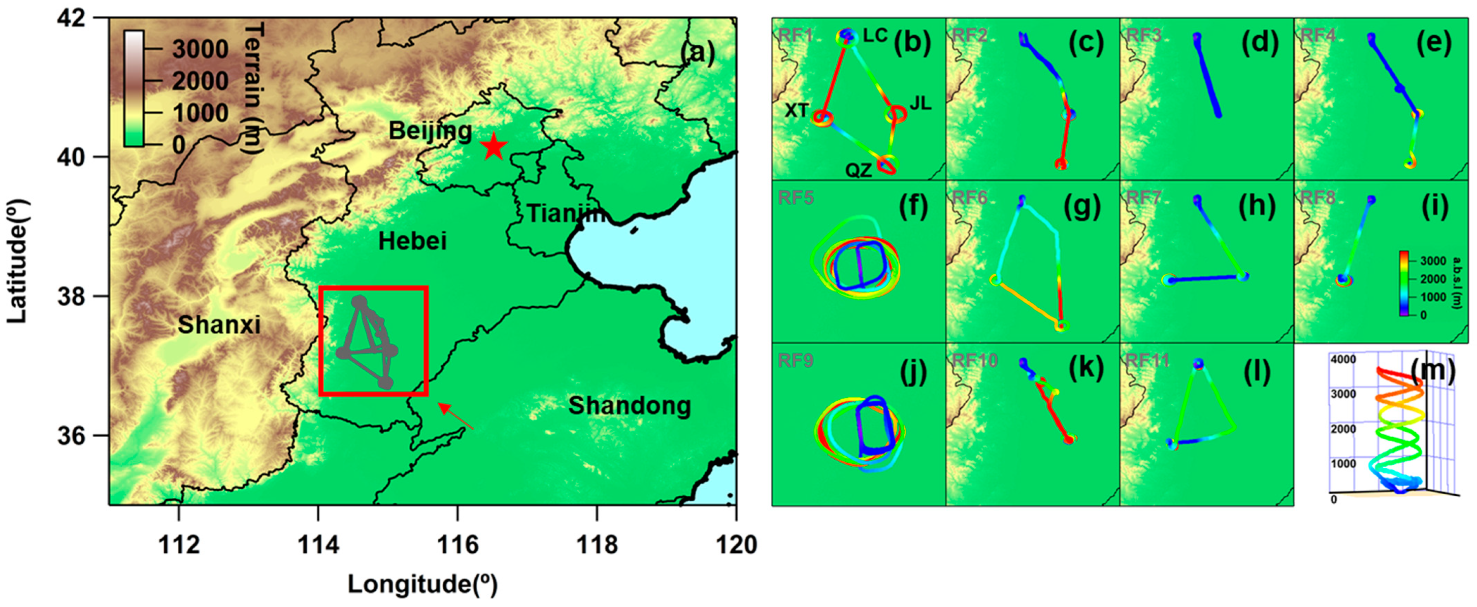
Experimental region	Hebei Province, China
IOP experiment duration	8 May to 11 June 2016
Aircraft	Y-12 research aircraft
Flight altitude	0.3~3.8 km above sea level
Total flights	11
Primary airborne instruments	Nephelometer, PSAP, CWIP, etc.
Primary ground-based instruments	MPL, CIMEL, etc.

and previous literature [2].

2.2. Supporting Data

2.2.1. Aircraft Instruments

The σ_sca and hemispheric backscattering coefficient (σ_bsca) were measured at three different wavelengths (450 nm, 550 nm, and 700 nm) using an integrating Nephelometer (Model 3565, TSI) from Y-12 aircraft. Details about the instrument introduction on calibration, uncertainties, and parameter settings are provided by references herein [34,35].

A particle soot absorption photometer (PSAP, Radiance Research, 565 nm) was used to measure highly sensitive σ_abs. The inlet was designed to pass aerosols up to ~4 micrometers in diameter. The observation principle and uncertainties of PSAP have been well documented [36,37]. The raw wavelengths of PSAP σ_abs (λ = 565 nm) were corrected to 550 nm by Equation (1) as below:

$${\mathit{\sigma }}_{\mathrm{abs}, {\mathit{\lambda }}_i}={\mathit{\sigma }}_{\mathrm{abs}, \mathit{\lambda }=565 nm}\times \frac{565}{{\mathit{\lambda }}_i}$$

(1)

where ${\mathit{\lambda }}_i$ is the ith wavelength.

The meteorological elements such as ambient temperature (T), relative humidity (RH), and pressure were measured by a cloud water inertial probe (CWIP, Rain Dynamics) installed on the Y-12 aircraft [2].

2.2.2. Ground Observation Instruments

A set of remote sensing instruments for measuring aerosol optical parameters has been installed on the Xingtai supersite. To characterize the aerosol extinction properties and the PBL structure [38,39], a micropulse lidar (MPL, manufactured by the Sigma Space Corporation (Lanham, MD, USA)) conducted ongoing observation during the experiment. It has an observational time resolution of 30 s and a vertical spatial resolution of 30 m, with a maximum detection altitude of approximately 20 km.

In order to assess AOD retrievals obtained from MPL, aircraft, and satellites, we implemented a CIMEL (CE-318) sun photometer, which is the standard instrument employed in AERONET. The CIMEL-retrieved AOD was acquired at eight channels (340, 380, 400, 500, 670, 870, 940, and 1020 nm). In addition, based on the spectral decomposition algorithm, the AERONET sites provide aerosol fine mode fraction (FMF) products from AOD measurements [40,41]. Under the quasi-static atmosphere assumption, a power law can be used to estimate the wavelength dependence of either σ_sca or AOD [42] as

$${\mathit{\sigma }}_{\mathit{\lambda }}={\mathit{\sigma }}_{{\mathit{\lambda }}_r}{(\frac{\mathit{\lambda }}{{\mathit{\lambda }}_r})}^{-\alpha \left(\frac{{\mathit{\lambda }}_1}{{\mathit{\lambda }}_2}\right)},$$

(2)

where σ_λ is σ_sca or AOD at a given reference wavelength (λ_r). α(λ₁/λ₂) is the dimensionless α, which corresponds to the slope of a double-logarithmic plot of wavelength. σ_sca or AOD can be calculated using Equation (3).

$$\alpha ({\lambda }_2/{\lambda }_1)=\frac{-\log ({\sigma }_{\mathrm{sca},{\lambda }_2}/{\sigma }_{\mathrm{sca}, {\lambda }_1})}{\log ({\lambda }_2/{\lambda }_1)}$$

(3)

The AOD at 550 nm was not obtained by the CIMEL photometer; it was calculated from AERONET α(440/675) data with λ_r = 500 nm using Equation (2). The retrieved AOD differs slightly when using either α(500/870), α(400/870), and α(380/500) instead of α(440/675), with the deviation below 1.2% at 550 nm.

2.2.3. Satellite Remote Sensing

For comparisons with airborne and ground-based measurements, the AODs were also retrieved from Moderate-Resolution Imaging Spectroradiometer (MODIS) Collection 5.1, L2 aerosol data, and Himawari-8 Geostationary Satellite (H8) Level 2 aerosol products. MODIS-retrieved AOD is commonly obtained using the dark target algorithm and the deep blue algorithm based on multiple channels [43]. The H8-AOD was retrieved from variables (0.47, 0.51, and 064 nm) and near-infrared (0.86 nm) [44]. In addition, the original H8-AOD at 500 nm was extrapolated to 550 nm by using α.

2.2.4. Other Data

The synoptic patterns used in this paper are concluded from the final reanalysis data provided by the National Center for Environmental Prediction (NCEP) (http://rda.ucar.edu/datasets/ds083.2/, accessed on 28 January 2024) with a spatial resolution of 1° × 1° and a time resolution of 6 h. The meteorological elements used in this paper (such as surface T, pressure, RH, WS, wind direction, visibility, etc.) are all from the meteorological observation network of the China Meteorological Administration.

3. Results

3.1. Airborne Measured Aerosol Optical Properties

The atmosphere was split into 100 m thick vertical layers, which were, based on weather conditions at flight time, categorized either as polluted profiles (PPs, defined as σ_sca > 100 Mm⁻¹) or clean profiles (CPs, all other layers) [2]. The layer closest to the surface was not considered.

Table 2. Flight summary and weather background.

NO.	Date	Spiral Region and Time Range (UTC)				Maximum Altitude (m)	Profile Type
		LC	JL	QZ	XT
RF1	20160508		a: 3:20–3:43 b: 2:56–3:20	a: 4:00–4:18	a: 4:40–4:55 b: 5:06–5:23 c: 5:23–5:42	3751	CPs
RF2	20160515		a: 4:42–5:05 b: 5:05–5:23	a: 5:58–6:18 b: 5:41–5:58		3679	Invalid data
RF3	20160516					467	Invalid data
RF4	20160517		a: 1:47–2:00	a: 2:18–2:29		2924	CPs
RF5	20160519	a: 7:43–8:02 b: 8:02–8:12 c: 8:29–8:35 d: 8:36–8:47 e: 8:47–9:08				3733	PPs
RF6	20160521			a: 5:00–5:16 b: 4:39–5:00	a: 5:51–6:06 b: 5:33–5:51 c: 6:06–6:16	3242	PPs
RF7	20160528		a: 4:28–4:40 b: 4:40–4:54 c: 4:54–5:00		a: 3:18–3:33 b: 3:53–4:11	3101	PPs
RF8	20160528				a: 9:15–9:30 b: 8:50–8:56 c: 9:39–9:54	3130	PPs
RF9	20160602	a: 5.47–6.07 b: 6:07–6:33				3591	Low-layer clean High-layer polluted
RF10	20160606		a: 3:03–3:19 b: 2:43–3:03			3178	PPs
RF11	20160611	a: 5:12–5:27 b: 5.45–5.48			a: 3:55–4:08 b: 4:24–4:44	3203	CPs

Different letters before the time range indicate the spiral profiles of aircraft measurement.

and Figure 1 show each profile’s spiral regions, time ranges, and atmospheric background (pristine or polluted) during the flight days. A total of 11 flights were conducted, and according to the ascent and descent of the aircraft, each flight profile is divided into separate spirals, such as RF1a, RF1b, etc. In addition to RF2 and RF3, which cannot be determined due to invalid data, there are 11 CPs for three flights and 22 PPs for six flights, respectively. For CPs, the mean value of σ_sca near the surface was 24.3 ± 4.4 Mm⁻¹, then grew slowly with height to ~50 Mm⁻¹ (750 m, ASL) and reached the maximum. Subsequently, σ_sca decreased gradually with altitude to 1/e of the near-surface value at ~2500 m (aerosol scale height). For PPs, the near-surface σ_sca was ~6 times greater than that of CPs, and the maximum value was ~206.3 ± 42.5 Mm⁻¹ at 900 m ASL.

The vertical distribution of σ_abs of PPs gradually decreased with height, which shows a significant difference from σ_abs of CPs, with the maximum value at the middle layer. The column-mean σ_abs of PPs (10.2 ± 8.1 Mm⁻¹) below 3000 m ASL was twice higher than that of CPs (4.8 ± 2.3 Mm⁻¹). Compared to the observation results of ACE-Asia, the maximum σ_abs is lower than most measurements, such as Xianghe (China) [45], Beijing (China) [46], and Kwangju (Korea) [5]. As we know, the concentration of black carbon is lowest in summer [47], and σ_abs may show an annual low during this campaign. It is interesting to note that while the trends in σ_abs and σ_sca were consistent across CPs, they exhibited significant variations in PPs during this campaign.

As shown in Figure 2, the vertical distribution of σ_ext (defined as the sum of σ_sca and σ_abs) depended on the vertical profile of σ_sca, especially on PPs. Combined with the vertical distribution of SSA, it indicates the significant contribution of scattering aerosols in the experimental region. The detailed calculation of σ_ext, α, and β_sca can refer to the previous study [2]. According to previous literature, α is an essential parameter that represents the size distribution of aerosols [48]. The pollution in the lower layer of PPs was likely caused by a higher concentration of fine-mode aerosols, characterized by a value of α close to ~2.0 with minimal standard deviations. The fluctuations of β_sca above 2000 m during the clean period indicate a rapid change in aerosol size, presumably due to the transport of airmasses.

A significant difference exists in the correlation between RH and σ_ext by dividing CPs and PPs during the field campaign. For CPs, the vertical distribution of σ_ext was distinctly different from RH (Figure 2i), and an inverse correlation between RH and σ_ext (R = 0.89) was found conspicuously by using curve fitting (Figure 3a). However, the distribution of σ_ext almost varied in harmony with RH in PPs, especially when the altitude was below 1000 m ASL. We adopted linear regression to represent the correlations between RH and σ_ext, and the correlation coefficients below and above 1000 m ASL were 0.88 and 0.96, respectively. To some extent, the combination of σ_ext and RHs high correlation, along with the associated information on airmass transport pathways [2], may serve as a reference for air quality forecasting in the NCP region.

3.2. Airborne Measured Aerosol Optical Properties

As the lowest portion of the troposphere, the structural and evolutionary characteristics of PBL are critical to the air contamination of urban areas [49]. PBL represents variable and sensitive coupling agents that regulate the fluxes of momentum, energy, and matter between the free troposphere and surface [50]. The height of the PBL is regarded as a critical element in estimating air pollution conditions, given the substantial correlation between the PBL and air contamination. H_PBL can be determined by the vertical distribution of the σ_ext, which is obtained from remote sensing observation (ground-based or satellite) or airborne in situ measurement. In addition, H_PBL can also be calculated using empirical formulas using ordinary meteorological observation data.

In this study, H_PBL obtained from airborne in situ measurement (H_PBL-airborne) is defined as the altitude where σ_sca decrease rate > 0.81 Mm⁻¹ m⁻¹ vertically [2]. The H_PBL-airborne of each flight spiral is shown in Figure 4, and the average H_PBL-airborne of 11 flights is ~1239 m ASL. Both the lowest (820 m ASL) and the highest (1910 m ASL) H_PBL-airborne were observed from the spirals over XT. The mean H_PBL-airborne of CPs and PPs is 1380 m and 1098 m ASL, respectively, indicating that lower H_PBL is more conducive to the accumulation and development of pollutants in this region. However, higher H_PBL may also be observed from PPs, such as XT-RF6a, where H_PBL-airborne is 1720 m ASL but under severe contamination. Conversely, the lowest H_PBL-airborne (820 m ASL, XT-RF1b) corresponded to a clean condition. While H_PBL serves as a significant indicator of atmospheric diffusion, it is influenced by intricate processes such as the horizontal and vertical wind fields, ambient RH, local emissions, and more, all of which shape the state of atmospheric pollution.

We analyzed the retrieved H_PBL (from ground-based MPL, XT) using the wavelet covariance transform method [51] from normalized relative backscatter (NRB) after eliminating the effects of the cloud. NRB signal is retrieved from MPL raw data after a series of data corrections, such as background noise correction, distance and energy normalization correction, resident pulse correction, etc. NRB is impacted by both the backscatter and extinction coefficient, and to some extent, it can reflect the aerosol’s spatial and temporal distribution. The step size of vertical resolution and NRB threshold were set to 210 m and 0.05, respectively. The first value from the lower layer exceeding this threshold or within a given threshold interval was considered H_PBL-MPL. For example, Figure 5 shows the retrieved NRB and the corresponding calculated H_PBL-MPL at XT on May 28. More complete descriptions are provided by references herein [52].

Figure 4. Comparison of airborne measured H_PBL, MPL retrieved H_PBL, and predicted H_PBL by meteorological data over Xingtai [53]. The dotted line was the average H_PBL observed by the aircraft. Different color represents the location of aircraft measurements.

Figure 4. Comparison of airborne measured H_PBL, MPL retrieved H_PBL, and predicted H_PBL by meteorological data over Xingtai [53]. The dotted line was the average H_PBL observed by the aircraft. Different color represents the location of aircraft measurements.

Using surface meteorological data to predict PBL structure by an empirical method [53] have significant application in the assessment of the regional PBL where no sounding observations are available. This method considers that PBL is formed by the combination of thermal and dynamic turbulence, and the motion in the upper part of the boundary layer is closely related to surface meteorological parameters. H_PBL can be obtained from a semi-empirical relation:

$$H_{\mathrm{PBL-predicted}}=\frac{121}{6}\left(6-P\right)\left(T-T_{\mathrm{d}}\right)+\frac{0.169 P\left(U_{\mathrm{Z}}+0.257\right)}{12 f\ln \left(Z/Z_0\right)}$$

(4)

where T_d is the surface dew point (K). U_z is the average wind speed (m s⁻¹) at height Z (m). Z₀ is the surface roughness (m). f is the ground rotation parameter (s⁻¹). P is the Pasquill stability level (atmospheric stability is divided into six levels: strong unstable = 1, unstable = 2, weakly unstable = 3, neutral = 4, more stable = 5, and stable = 6).

In this study, we use airborne measured profiles to verify the predicted H_PBL (H_{PBL-predicted}) and ground-based retrieved H_PBL-MPL. Figure 6 shows the scatterplot of H_PBL-airborne as a function of H_PBL-MPL and H_{PBL-predicted} over XT during the field campaign. All these H_PBL data are consistently converted spatiotemporally to match each other. In general, H_PBL derived from aircraft and MPL followed the same trends over XT, except for XT-RF7a, XT-RF11a, and XT-RF11b. H_PBL-MPL was slightly higher than H_PBL-airborne. A linear regression shows the correlation between H_PBL-airborne and H_PBL-MPL, R = 0.89 (Figure 6a). As shown in Figure 6b, H_{PBL-predicted} agrees well with H_PBL-airborne (R = 0.76), with the differences between them typically within a range of dozens to a few hundred meters. While H_{PBL-predicted} values can indicate the variation tendency of H_PBL, the actual values tend to be underestimated (~192 m on average) to some extent. Particularly during haze episodes, the average underestimation of H_{PBL-predicted} is ~260 m, compared to ~72 m during the clean period.

3.3. Comparison of Multi-Source Retrieved AOD

Most pollutants resided below the maximum flight height in the vertical profiles of airborne measured aerosol optical properties. The aircraft-retrieved AOD (aircraft-AOD) was calculated by integrating σ_sca over flight height, according to Wang et al. [2] in this study. Figure 7 shows the aircraft-AOD of each vertical profile at every 1000 m altitude range and the whole layer during the experiment. As a result of the aerosol accumulation in the PBL, AOD values exceeding 0.1 were primarily distributed below 2000 m ASL, particularly during pollution episodes when AOD decreased considerably with altitude. In the context of clean air, AOD variation is minimal and slightly decreases with height, exhibiting a notable contrast to the pollution period. However, we noticed in the vertical profiles obtained by LC-RF9a and LC-RF9b on 2 June that aircraft-AOD increased with altitude. This increase was likely due to PM transmission in the upper layer.

The AERONET-retrieved AOD (AERONET-AOD) at 550 nm was calculated by Equation (2) and compared with six aircraft-AOD vertical profiles of over XT. AERONET-AOD and aircraft-AOD show a good correlation (R = 0.91), and AERONET-AOD is about 1.4 times higher on average than aircraft-AOD, probably due to the limitation of flight height. We utilized the fine mode fraction (FMF) derived from AERONET to obtain the contribution of fine particles to AOD (AOD_f = AOD × FMF) during the field campaign. Take the FMF products from the AERONET website as an example. Figure 8a shows the retrieved aerosol volume spectrum distribution under clean (corresponding to CPs on 17 May) and polluted (corresponding to PPs on 28 May) conditions, respectively. Figure 8b displays the mean FMF corresponding to CPs and PPs. Note that AOD_f was closed to AOD under PPs conditions, with FMF > 0.8, indicating a significant contribution of fine particles in the NCP region. Observing the variation from XT-RF7b to XT-RF8a (two research flights were conducted over XT on 28 May), it is evident that there was a shift from pollution to cleanliness during this period, resulting in a drastic decrease in FMF from 0.88 to 0.58.

Figure 9a–c shows the correlation relationship between aircraft-AOD and ground-based AOD measurements. For MPL-retrieved AOD (MPL-AOD), it has the best correlation with aircraft-AOD, and both exhibited a similar tendency, especially at altitudes above 1000 m ASL (R = 0.97). In terms of value, the MPL-AOD is generally higher than the aircraft-AOD at each layer. Among them, at altitudes between 0 and 1000 m ASL, the MPL-AOD is on average 1.7 times greater than that of aircraft-AOD, while at altitudes between 1000 m and 2000 m ASL, it is 1.5 times greater. There is no significant difference between the two above 2000 m ASL (Figure 7). It is speculated that the reason for the overestimation of MPL-AOD is primarily influenced by the AOD inversion algorithm and the cloud identification algorithm.

Aiming to provide spatial coverage for the observation of atmospheric parameters, satellite remote sensing plays a more and more important role in environmental monitoring [41]. However, there is an ongoing critical need to validate the satellite retrieval by in-situ measurements such as airborne and ground-based observation. In this study, we compared the satellite-retrieved AOD from MODIS [including the Dark Target (DT) and Deep Blue (DB) algorithms] and H8 official products with the simultaneous measurement AOD from this experiment. There are 38 airborne profiles selected for comparison with MODIS and H8 official products. The matching approach involves taking the center point of a spiral as the pivot point, and the compared satellite AOD is an average result from MODIS or H8 within the nine grid points surrounding the pivot point. If more than half of the grid AOD within the specified scope is deficient, it is recorded as a missing measurement. Figure 9d–f shows the correlation relationship between aircraft-AOD and satellite-retrieved AOD. Clean and polluted conditions are also separate for comparison. Both MODIS-AOD and H8-AOD vary widely, ranging from 0.05~2, which were significantly larger than aircraft-AOD (ranging from 0~1). The correlation between satellite-retrieved AOD and aircraft-derived AOD is generally low compared to ground-based AOD measurements. Only MODIS-DT-AOD exhibited a relatively better correlation with aircraft-AOD, R = 0.7. There are many factors that influence the satellite-retrieved AOD. In addition to the accuracy of the inversion algorithm, the remote sensing method is also sensitive to the representativeness of the space. This means that it responds to the average state of a certain range with greater uncertainty for small-scale studies. The observation results for H8 are significantly impacted by the measured angle and, simultaneously, by the solar altitude angle. The daily variation of AOD is significant, and the retrieved value is generally higher in the afternoon. However, this research flights for this experiment were primarily conducted in the afternoon (local time). Hence, this likely explains the reason for the discrepancies between the AOD values retrieved from satellites and those measured by aircraft. More in-depth quantitative analysis is certainly needed to examine this.

4. Conclusions

In this study, multi-source measurements such as aircraft, ground-based remote sensing, and satellite observations are utilized to compare and analyze the vertical information of aerosol optical properties in the NCP region from May to June 2016. We discuss the PBL and AOD characteristics during the in-situ experiment by considering the specific observation region and the corresponding atmospheric background (pristine or polluted). This study yields several key findings and conclusions.

Airborne measured aerosol optical properties such as σ_sca, σ_abs, σ_ext, SSA, α, and β_sca were analyzed by separating the vertical profiles into CPs and PPs. σ_sca, σ_abs, and σ_ext gradually decrease with altitude increasing, with the exception of σ_abs of PPs, which reach their maximum point near-surface, and other parameters’ peak values all near H_PBL. The average near-surface σ_sca of PPs was ~6 times greater than that of CPs, and its maximum value was ~206.3 ± 42.5 Mm⁻¹ at 900 m ASL. The column-mean σ_abs of PPs (10.2 ± 8.1 Mm⁻¹) below 3000 m was twice higher than that of CPs (4.8 ± 2.3 Mm⁻¹). The vertical profiles of σ_ext depended most on the vertical distribution of measured σ_sca, which indicates a significant contribution of scattering aerosols in the experimental region. The pollution in the lower layer of PPs was likely caused by the accumulation of fine-mode aerosols, characterized by a value of α close to ~2.0 with minimal standard deviations. The analysis of AERONET-FMF products in Section 3.3 also confirms this viewpoint. The fluctuations of β_sca above 2000 m during the clean period indicate a rapid change in aerosol size, presumably due to the transport of airmasses. In addition, σ_ext exhibited an opposite relationship with RH in the case of CPs and PPs. The combination of σ_ext and RH may serve as a reference for air quality forecasting in the NCP region.

The average H_PBL-airborne distance of 11 research flights is ~1239 m ASL. In general, the H_PBL derived from aircraft and MPL vary in harmony over the XT region. H_PBL-MPL was slightly higher than H_PBL-airborne, and the correlation coefficient was ~0.89. H_PBL predicted by using surface meteorological data can indicate the trend of variation in H_PBL; however, the actual values tend to be underestimated to some extent. Particularly during haze episodes, the average underestimation of H_{PBL-predicted} is ~260 m, compared to ~72 m during the clean period.

The comparison and discussion of AOD from multi-source measurements were also involved in this study. AERONET-AOD and aircraft-AOD show a good correlation (R = 0.91), and AERONET-AOD is about 1.4 times higher on average than aircraft-AOD, probably due to the limitation of flight height. Fine-mode particles contribute the most in the experimental region, according to the analysis of AERONET FMF products. For MPL-retrieved AOD, it has the best correlation with aircraft-AOD, and both exhibited a similar tendency. However, the AOD inversion algorithm and cloud identification algorithm of MPL may cause an overestimation of MPL-AOD under certain circumstances. Thirty-eight airborne profiles were selected for comparison with MODIS and H8 official AOD products. Both MODIS-AOD and H8-AOD were significantly larger than aircraft-AOD, and only MODIS-DT-AOD exhibited a relatively better correlation with aircraft-AOD. There are many factors that influence the satellite-retrieved AOD. In addition to the accuracy of the inversion algorithm, the remote sensing method is also sensitive to the representativeness of the space. More observational cases and delving deeper into quantitative analysis are certainly needed to investigate this.

References

- Zhang, Q.; Streets, D.G.; He, K.; Wang, Y.; Richter, A.; Burrows, J.P.; Uno, I.; Jang, C.J.; Chen, D.; Yao, Z.; et al. NOx emission trends for China, 1995–2004: The view from the ground and the view from space. J. Geophys. Res. 2007, 112, D22306. [Google Scholar] [CrossRef]
- Wang, F.; Li, Z.; Ren, X.; Jiang, Q.; He, H.; Dickerson, R.R.; Dong, X.; Lv, F. Vertical distributions of aerosol optical properties during the spring 2016 ARIAs airborne campaign in the North China Plain. Atmos. Chem. Phys. 2018, 18, 8995–9010. [Google Scholar] [CrossRef]
- Zhang, R.; Wang, Y.; Li, Z.; Wang, Z.; Dickerson, R.R.; Ren, X.; He, H.; Wang, F.; Gao, Y.; Chen, X.; et al. Vertical profiles of cloud condensation nuclei number concentration and its empirical estimate from aerosol optical properties over the North China Plain. Atmos. Chem. Phys. 2022, 22, 14879–14891. [Google Scholar] [CrossRef]
- Wang, Y.; Li, Z.; Zhang, Y.; Du, W.; Zhang, F.; Tan, H.; Xu, H.; Fan, T.; Jin, X.; Fan, X. Characterization of aerosol hygroscopicity, mixing state, and CCN activity at a suburban site in the central North China Plain. Atmos. Chem. Phys. 2018, 18, 11739–11752. [Google Scholar] [CrossRef]
- Kim, D.H.; Sohn, B.J.; Nakajima, T.; Takamura, T.; Takemura, T.; Choi, B.C.; Yoon, S.C. Aerosol optical properties over east Asia determined from ground-based sky radiation measurements. J. Geophys. Res. 2004, 109, 127–142. [Google Scholar] [CrossRef]
- Chameides, W.L.; Yu, H.; Liu, S.C.; Bergin, M.; Zhou, X.; Mearns, L.; Wang, G.; Kiang, C.S.; Saylor, R.D.; Luo, C. Case Study of the Effects of Atmospheric Aerosols and Regional Haze on Agriculture: An Opportunity to Enhance Crop Yields in China through Emission Controls? Proc. Natl. Acad. Sci. USA 1999, 96, 13626–13633. [Google Scholar] [CrossRef]
- Bellouin, N.; Boucher, O.; Haywood, J.; Reddy, M.S. Global estimate of aerosol direct radiative forcing from satellite measurements. Nature 2005, 438, 1138–1141. [Google Scholar] [CrossRef] [PubMed]
- Nair, V.S.; Babu, S.S.; Moorthy, K.K.; Sharma, A.K.; Marinoni, A.; Ajai. Black carbon aerosols over the Himalayas: Direct and surface albedo forcing. Tellus Ser. B-Chem. Phys. Meteorol. 2013, 65, 129–133. [Google Scholar] [CrossRef]
- Horvath, H. Estimation of the average visibility in central Europe. Atmos. Environ. 1995, 29, 241–246. [Google Scholar] [CrossRef]
- Ramanathan, V.; Crutzen, P.J. New Directions: Atmospheric Brown “Clouds”. Atmos. Environ. 2003, 37, 4033–4035. [Google Scholar] [CrossRef]
- Moorthy, K.K.; Nair, V.S.; Babu, S.; Satheesh, S. Spatial and vertical heterogeneities in aerosol properties over oceanic regions around India: Implications for radiative forcing. Q. J. R. Meteorol. Soc. 2009, 135, 2131–2145. [Google Scholar] [CrossRef]
- Lawrence, M.G.; Lelieveld, J. Atmospheric pollutant outflow from southern Asia: A review. Atmos. Chem. Phys. 2010, 10, 11017–11096. [Google Scholar] [CrossRef]
- Sun, Y.; Jiang, Q.; Xu, Y.; Ma, Y.; Zhang, Y.; Liu, X.; Li, W.; Wang, F.; Li, J.; Wang, P. Aerosol characterization over the North China Plain: Haze life cycle and biomass burning impacts in summer. J. Geophys. Res. Atmos. 2016, 121, 2508–2521. [Google Scholar] [CrossRef]
- Han, T.; Xu, W.; Chen, C.; Liu, X.; Wang, Q.; Li, J.; Zhao, X.; Du, W.; Wang, Z.; Sun, Y. Chemical apportionment of aerosol optical properties during the Asia-Pacific Economic Cooperation summit in Beijing, China. J. Geophys. Res. Atmos. 2016, 120, 12281–12295. [Google Scholar] [CrossRef]
- Babu, S.S.; Nair, V.S.; Gogoi, M.M.; Moorthy, K.K. Seasonal variation of vertical distribution of aerosol single scattering albedo over Indian sub-continent: RAWEX aircraft observations. Atmos. Environ. 2016, 125, 312–323. [Google Scholar] [CrossRef]
- Li, Z.; Ying, Z.; Jie, S.; Li, B.; Jin, H.; Dong, L.; Li, D.; Peng, W.; Wei, L.; Lei, L. Remote sensing of atmospheric particulate mass of dry PM2.5 near the ground: Method validation using ground-based measurements. Remote Sens. Environ. 2016, 173, 59–68. [Google Scholar] [CrossRef]
- Zhao, P.; Yin, Y.; Xiao, H. The Effects of Aerosol on Development of Thunderstorm Electrification: A Numerical Study. Atmos. Res. 2015, 153, 376–391. [Google Scholar] [CrossRef]
- Li, Z.; Wang, Y.; Guo, J.; Zhao, C.; Cribb, M.C.; Dong, X.; Fan, J.; Gong, D.; Huang, J.; Jiang, M. East asian study of tropospheric aerosols and their impact on regional clouds, precipitation, and climate (EAST-AIRCPC). J. Geophys. Res. Atmos. 2019, 124, 13026–13054. [Google Scholar] [CrossRef]
- Li, Z.; Rosenfeld, D.; Fan, J. Aerosols and their impact on radiation, clouds, precipitation, and severe weather events. In Oxford Research Encyclopedia of Environmental Science; Oxford University Press: Oxford, MI, USA, 2017. [Google Scholar]
- Li, Z.; Guo, J.; Ding, A.; Liao, H.; Liu, J.; Sun, Y.; Wang, T.; Xue, H.; Zhang, H.; Zhu, B. Aerosol and boundary-layer interactions and impact on air quality. Natl. Sci. Rev. 2017, 4, 810–833. [Google Scholar] [CrossRef]
- Haywood, J.; Boucher, O. Estimates of the direct and indirect radiative forcing due to tropospheric aerosols: A review. Rev. Geophys. 2000, 38, 513–543. [Google Scholar] [CrossRef]
- Lau, K.M.; Kim, M.K.; Kim, K.M. Asian summer monsoon anomalies induced by aerosol direct forcing: The role of the Tibetan Plateau. Clim. Dyn. 2006, 26, 855–864. [Google Scholar] [CrossRef]
- Liu, J.; Zheng, Y.; Li, Z.; Cribb, M. Analysis of cloud condensation nuclei properties at a polluted site in southeastern China during the AMF-China Campaign. J. Geophys. Res. Atmos. 2011, 116, D00K35. [Google Scholar] [CrossRef]
- Anderson, T.L.; Masonis, S.J.; Covert, D.S.; Ahlquist, N.C.; Howell, S.G.; Clarke, A.D.; McNaughton, C.S. Variability of aerosol optical properties derived from in situ aircraft measurements during ACE-Asia. J. Geophys. Res. Atmos. 2003, 108, D23. [Google Scholar] [CrossRef]
- John, M.L.; Philip, B.R.; Jeffrey, S.R.; Jens, R.; Beat, S.; Duane, A.A.; Omar, T.; Robert, C.L.; Lorraine, A.R.; Brent, N.H.; et al. Airborne Sun photometer measurements of aerosol optical depth and columnar water vapor during the Puerto Rico Dust Experiment and comparison with land, aircraft, and satellite measurements. J. Geophys. Res. 2003, 108, D19. [Google Scholar] [CrossRef]
- Sun, Y.; Du, W.; Fu, P.; Wang, Q.; Li, J.; Ge, X.; Zhang, Q.; Zhu, C.; Ren, L.; Xu, W. Primary and secondary aerosols in Beijing in winter: Sources, variations and processes. Atmos. Chem. Phys. 2016, 16, 8309–8329. [Google Scholar] [CrossRef]
- Jiang, Q.; Sun, Y.; Wang, Z.; Yin, Y. Aerosol composition and sources during the Chinese Spring Festival: Fireworks, secondary aerosol, and holiday effects. Atmos. Chem. Phys. 2015, 15, 6023–6034. [Google Scholar] [CrossRef]
- Wang, Q.; Sun, Y.; Xu, W.; Du, W.; Zhou, L.; Tang, G.; Chen, C.; Cheng, X.; Zhao, X.; Ji, D. Vertically resolved characteristics of air pollution during two severe winter haze episodes in urban Beijing, China. Atmos. Chem. Phys. 2018, 18, 2495–2509. [Google Scholar] [CrossRef]
- Garland, R.M.; Schmid, O.; Nowak, A.; Achtert, P.; Wiedensohler, A.; Gunthe, S.S.; Takegawa, N.; Kita, K.; Kondo, Y.; Hu, M. Aerosol optical properties observed during Campaign of Air Quality Research in Beijing 2006 (CAREBeijing-2006): Characteristic differences between the inflow and outflow of Beijing city air. J. Geophys. Res. Atmos. 2009, 114, 1065–1066. [Google Scholar] [CrossRef]
- Dong, Z.; Li, Z.; Yu, X.; Cribb, M.; Li, X.; Dai, J. Opposite long-term trends in aerosols between low and high altitudes: A testimony to the aerosol–PBL feedback. Atmos. Chem. Phys. 2017, 17, 7997–8009. [Google Scholar] [CrossRef]
- Barbaro, E.; Vilà-Guerau de Arellano, J.; Krol, M.; Holtslag, A. Impacts of aerosol shortwave radiation absorption on the dynamics of an idealized convective atmospheric boundary layer. Bound.-Layer Meteorol. 2013, 148, 31–49. [Google Scholar] [CrossRef]
- Ge, B.; Wang, Z.; Lin, W.; Xu, X.; Li, J.; Ji, D.; Ma, Z. Air pollution over the North China Plain and its implication of regional transport: A new sight from the observed evidences. Environ. Pollut. 2018, 234, 29–38. [Google Scholar] [CrossRef] [PubMed]
- Wang, L.; Li, P.; Yu, S.; Mehmood, K.; Li, Z.; Chang, S.; Liu, W.; Rosenfeld, D.; Flagan, R.C.; Seinfeld, J.H. Predicted impact of thermal power generation emission control measures in the Beijing-Tianjin-Hebei region on air pollution over Beijing, China. Sci. Rep. 2018, 8, 934. [Google Scholar] [CrossRef]
- Anderson, T.L.; Covert, D.S.; Marshall, S.F.; Laucks, M.L.; Charlson, R.J.; Waggoner, A.P.; Ogren, J.A.; Caldow, R.; Holm, R.L.; Quant, F.R. Performance Characteristics of a High-Sensitivity, Three-Wavelength, Total Scatter/Backscatter Nephelometer. J. Atmos. Ocean. Technol. 2009, 13, 967. [Google Scholar] [CrossRef]
- Anderson, T.L.; Ogren, J.A. Determining Aerosol Radiative Properties Using the TSI 3563 Integrating Nephelometer. Aerosol Sci. Technol. 1998, 29, 57–69. [Google Scholar] [CrossRef]
- Bond, T.C.; Anderson, T.L.; Campbell, D. Calibration and Intercomparison of Filter-Based Measurements of Visible Light Absorption by Aerosols. Aerosol Sci. Technol. 1999, 30, 582–600. [Google Scholar] [CrossRef]
- Sheridan, P.J.; Arnott, W.P.; Ogren, J.A.; Andrews, E.; Atkinson, D.B.; Covert, D.S.; Moosmüller, H.; Petzold, A.; Schmid, B.; Strawa, A.W. The Reno Aerosol Optics Study: An Evaluation of Aerosol Absorption Measurement Methods. Aerosol Sci. Technol. 2005, 39, 1–16. [Google Scholar] [CrossRef]
- Wang, Y.; Zhao, C.; Dong, Z.; Li, Z.; Hu, S.; Chen, T.; Tao, F.; Wang, Y. Improved retrieval of cloud base heights from ceilometer using a non-standard instrument method. Atmos. Res. 2018, 202, 148–155. [Google Scholar] [CrossRef]
- Zhao, C.; Wang, Y.; Wang, Q.; Li, Z.; Wang, Z.; Liu, D. A new cloud and aerosol layer detection method based on micropulse lidar measurements. J. Geophys. Res. Atmos. 2014, 119, 6788–6802. [Google Scholar] [CrossRef]
- O’neill, N.; Eck, T.; Smirnov, A.; Holben, B.; Thulasiraman, S. Spectral discrimination of coarse and fine mode optical depth. J. Geophys. Res. Atmos. 2003, 108, D17. [Google Scholar] [CrossRef]
- Zhang, Y.; Li, Z. Remote sensing of atmospheric fine particulate matter (PM2.5) mass concentration near the ground from satellite observation. Remote Sens. Environ. 2015, 160, 252–262. [Google Scholar] [CrossRef]
- Ångström, A. The parameters of atmospheric turbidity. Tellus 1964, 16, 64–75. [Google Scholar] [CrossRef]
- Kaufman, Y.J.; Fraser, R.S. The effect of smoke particles on clouds and climate forcing. Science 1997, 277, 1636–1639. [Google Scholar] [CrossRef]
- Fukuda, S.; Nakajima, T.; Takenaka, H.; Higurashi, A.; Kikuchi, N.; Nakajima, T.Y.; Ishida, H. New approaches to removing cloud shadows and evaluating the 380 nm surface reflectance for improved aerosol optical thickness retrievals from the GOSAT/TANSO-Cloud and Aerosol Imager. J. Geophys. Res. Atmos. 2013, 118, 13520–13531. [Google Scholar] [CrossRef]
- Li, C.; Marufu, L.T.; Dickerson, R.R.; Li, Z.; Wen, T.; Wang, Y.; Wang, P.; Chen, H.; Stehr, J.W. In situ measurements of trace gases and aerosol optical properties at a rural site in northern China during East Asian Study of Tropospheric Aerosols: An International Regional Experiment 2005. J. Geophys. Res. Atmos. 2007, 112, D22S04. [Google Scholar] [CrossRef]
- Bergin, M.; Cass, G.; Xu, J.; Fang, C.; Zeng, L.; Yu, T.; Salmon, L.; Kiang, C.; Tang, X.; Zhang, Y. Aerosol radiative, physical, and chemical properties in Beijing during June 1999. J. Geophys. Res. Atmos. 2001, 106, 17969–17980. [Google Scholar] [CrossRef]
- Garland, R.M.; Yang, H.; Schmid, O.; Rose, D. Aerosol optical properties in a rural environment near the mega-city Guangzhou, China: Implications for regional air pollution and radiative forcing. Atmos. Chem. Phys. 2008, 8, 5161–5186. [Google Scholar] [CrossRef]
- Hamonou, E.; Chazette, P.; Balis, D.; Dulac, F.; Schneider, X.; Galani, E.; Ancellet, G.; Papayannis, A. Characterization of the vertical structure of Saharan dust export to the Mediterranean basin. J. Geophys. Res. Atmos. 1999, 104, 22257–22270. [Google Scholar]
- Xu, D.; Wang, Y.; Zhu, R. Atmospheric environmental capacity and urban atmospheric load in mainland China. Sci. China Earth Sci. 2018, 61, 33–46. [Google Scholar] [CrossRef]
- Miao, Y.; Liu, S. Linkages between aerosol pollution and planetary boundary layer structure in China. Sci. Total Environ. 2019, 650, 288–296. [Google Scholar] [CrossRef]
- Gamage, N.; Hagelberg, C. Detection and analysis of microfronts and associated coherent events using localized transforms. J. Atmos. Sci. 1993, 50, 750–756. [Google Scholar] [CrossRef]
- Li, X.; Quan, J.; Wang, F.; Sheng, J.; Gao, Y.; Zhao, D.; Cheng, Z. Evaluation of the method for planetary boundary layer height retrieval by lidar and its application in Beijing. Chin. J. Atmos. Sci. 2018, 42, 435–446. [Google Scholar]
- Nozaki, K. Mixing depth model using hourly surface observations. USAF Environ. Tech. Appl. Cent. Rep. 1973, 7053, 25. [Google Scholar]