On the Consistency of Stochastic Noise Properties and Velocity Estimations from Different Analysis Strategies and Centers with Environmental Loading and CME Corrections

Abstract

The analysis of the Global Navigation Satellite System (GNSS) time series provides valuable information for geodesy and geodynamics research. Precise data analysis strategies are crucial for accurately obtaining the linear velocity of GNSS stations, enabling high-precision applications of GNSS time series. This study investigates the impact of different stochastic noise models on velocity estimations derived from GNSS time series, specifically under conditions of environmental loading correction and common mode error (CME) removal. By comparing data from various data centers, we find that post-correction, different analysis strategies exhibit high consistency in their noise characteristics and velocity estimation results. Across various analysis strategies, the optimal noise models were predominantly Power Law with White Noise (PLWN) and Flicker Noise with White Noise (FNWN), with the optimal noise models including COMB/JPL, COMB/SOPAC, and COMB/NGL for approximately 50% of the datasets. Most of the stations (approximately 80%) showed velocity differences below 0.3 mm/year and velocity estimation uncertainties below 0.1 mm/year. Nonetheless, variations in amplitudes and periodic signals persisted due to differences in the processing of raw GNSS observations. For instance, the NGL and JPL datasets, which were processed using GipsyX 2.1 software, showed higher amplitudes of the 5.5-day periodic signal. These findings provide a solid empirical foundation for advancing data analysis methods and enhancing the reliability of GNSS time series results in future research.

1. Introduction

In the past two decades, the Global Navigation Satellite System (GNSS) has led to significant advancements in measurement precision and accuracy [1,2,3]. As a consequence, there are several geodynamic processes that are now observed using the GNSS technique. Moreover, GNSS time series contain many useful signals, reflecting not only the linear trends associated with uplift and subsidence but also the nonlinear variations caused by geophysical effects. For instance, GNSS position solutions have been used in the study of geophysical phenomena, such as plate tectonics [4,5,6,7,8], crustal deformation caused by earthquakes [9,10], drought monitoring [11,12,13], glacial isostatic adjustment [14,15,16], and vertical crustal deformation to study sea level variations [17,18,19,20].

Accurately separating nonlinear signals from the GNSS time series is crucial for achieving precise estimates of the linear velocity of GNSS stations. Numerous studies indicate various pseudo-periodic signals in GNSS time series, including annual and semi-annual variations [21,22,23,24,25]. The majority of these annual signals have been validated as authentic station displacements, whereas certain seasonal signals may be related to geophysical factors associated with hydrological loading, atmospheric loading, non-tidal oceanic loading, etc. Periodic global-scale shifts in surface loading contribute to mass redistribution across the Earth’s surface, thereby inducing corresponding changes. The influence of surface loading introduces biases in station displacements and velocity estimates [1,22,26,27,28]. Spatially and temporally correlated errors among GNSS networks are called Common Mode Error (CME) [26,29,30,31]. The source of many of these CMEs remains uncertain, but they potentially arise from residual model errors or unmodeled disturbances. The presence of a CME can obscure weak or transient structural signals, significantly impacting the extraction of deformation characteristics across different parts of a region.

High-precision data processing software is essential for achieving reliable solutions. Due to varying models, data analysis strategies, and other factors, different software packages may introduce systematic differences in computed results, thereby yielding time series with distinct temporal characteristics. Studies comparing the results processed with GAMIT and GipsyX have indicated that despite exhibiting similar root mean square errors (RMSEs) at comparable levels, differences in processing modes can still lead to systematic discrepancies. Similarly, systematic differences have been observed between the results obtained from Bernese and GipsyX, even when using the same software [3]. Variations in computation and analysis strategies, such as the selection of different ionospheric and tropospheric correction models, the degree of constraint that is applied to reference station coordinates and satellite orbits, the choice of force models, and methods for cycle slip repair, can significantly impact the results. These factors contribute to systematic errors in the solutions in terms of both scale and direction [32].

Mismodeling effects can also lead to spurious periodic signals. For instance, the repeat period of satellite orbits (known as the draconitic year, approximately 351.2 ± 2.8 days) can be transmitted to station positions through the relative positioning relationship between reference stations and satellites, manifesting as false periodic signals and their harmonics (e.g., 1.04 cycles per year, approximately 351.2 days). This phenomenon is observed in nearly all IGS products [23]. Errors stemming from imperfect modeling or mis-modeling processes, such as ocean tides or tropospheric and ionospheric delay errors in precise GNSS data processing stages, can similarly introduce false periodic signals into time series. Studies have found that unmodeled errors in the weekly and semi-weekly tidal frequency bands can have long-term effects, resulting in false signals resembling bi-weekly, semi-annual, and annual variations in time series. This can lead to erroneous interpretations of geophysical signals [33,34]. Abraha [35] demonstrated that errors in GLONASS orbits include periodic signals with an 8-day cycle. When GPS and GLONASS are jointly processed in coordinate products or when GPS orbits are derived from combined GPS and GLONASS processing, these errors can propagate into station coordinates.

Kall et al. [36] analyzed the influence of the GipsyX and Bernese processing software packages on the noise characteristics and velocity estimations of GNSS stations in the Estonian region. They revealed that while the velocity estimations from GipsyX and Bernese are consistent in the E and U components, a systematic bias exists in the N component. Furthermore, through a comparison of periodic signals derived from different analysis strategies, Bogusz et al. [37] identified systematic differences between NGL and IGS, which are likely attributable to variations in the reference frame alignment strategies employed. Despite offering valuable insights, these studies have certain limitations. First, there is a lack of systematic analysis regarding the consistency of noise characteristics and velocity estimation results across different analysis centers and analysis strategies. Second, the effects of environmental loading corrections and the removal of CMEs on the consistency of the results remain underexplored. To address these gaps, this study compares GNSS velocity estimations and stochastic noise characteristics derived from various analysis centers and strategies, with a particular focus on cases where environmental loading and CME corrections are applied. By utilizing multiple noise models and data analysis strategies, we investigate the consistency of data across different analysis strategies and delve into the underlying causes of the discrepancies. These findings contribute for elucidating the relationship between environmental loading, CMEs, and data analysis strategies, enabling the precise separation of nonlinear motions in GNSS time series and supporting the development of high-precision GNSS applications.

This paper is organized as follows. Section 2 provides a brief introduction to the GNSS data and analysis strategies for these and describes the environmental loading data and the methods employed in this study. Section 3 presents a consistency analysis of data processed using different strategies. Finally, concluding remarks are given in Section 5.

2. Materials and Methods

2.1. GNSS Time Series

The GNSS time series selected for this study are derived from the “Clean_Detrend” daily position time series within the global IGS14 framework provided by the Scripps Orbit and Permanent Array Center (SOPAC) (http://sopac.ucsd.edu/, accessed on 9 November 2023) and the daily position time series provided by the Nevada Geodetic Laboratory (NGL) (http://geodesy.unr.edu/index.php, accessed on 9 November 2023). The SOPAC offers three types of GNSS time series products: the JPL time series, computed using Gipsy X Network Processor (NWPx) software version 2.1; the SOPAC time series, computed using GAMIT/GLOBK 10.71; and the COMB time series, obtained by jointly processing the JPL and SOPAC data. Detailed strategies for data processing [3,38,39] are outlined in

Table 1. Different data analysis strategies.

Solutions	JPL GIPSY Analysis	SOPAC GAMIT Analysis	NGL GIPSY Analysis
Earth tides	IERS 2010 convention	IERS 2010 convention	IERS 2010 convention
Ocean tidal loading	IERS 2010 convention	FES04 model with the center of mass correction	Diurnal, semidiurnal, MF, and MM Model:FES04
Pole tide	IERS 2010 convention	IERS 2010 convention	IERS 2010 convention
Tropospheric mapping function	GPT2w tropospheric mapping function	VMF1 tropospheric mapping function	VMF1 tropospheric mapping function
General relativity effect	Periodic clock corrections and gravity-bending corrections applied	IERS 2010 convention	Periodic clock corrections, Shapiro Delay

. As shown in Figure 1, the time series produced using different strategies exhibit high consistency in the EN components, while some differences are observed in the U component.

The JPL time series [3,38] is estimated using the Gipsy X Network Processor (NWPx), which runs the GipsyX 2.1. The NWPx was developed to analyze daily positions for large GNSS networks using precise point positioning (PPP) with ambiguity resolution in a no-net-rotation frame, which was later transformed into the IGS realization of the ITRF. In the PPP strategy, satellite clocks and orbits are fixed to the values provided from a separate precise orbit determination process. Its advantages include high computational efficiency and a significant reduction in error sources. Additionally, the quality of observations is not affected by the quality of observations at individual stations.

The SOPAC time series [3,38] is estimated using the GAMIT/GLOBK 10.71 processing software using a double-differenced mode. The main steps involve initially computing the baseline’s respective coordinates and the satellite orbits’ daily relaxed solution using a carrier phase and pseudorange data in a double-differenced strategy. Subsequently, the obtained daily relaxed solution is merged with the global IGS station’s daily relaxed solution to derive a combined relaxed solution. Finally, a Kalman filtering method is applied to estimate the station’s position and velocity.

The COMB time series [38] combines the “post-ATS SOPAC” and “JPL Raw_M XYZ” time series using a weighted mean algorithm to achieve a time series with higher precision than independent solutions from the JPL and SOPAC. The algorithm is performed on a station-by-station basis, assuming that there are no correlations between stations but using the variance–covariance matrices for each solution. Temporal correlations (colored noise) are taken into consideration when assigning uncertainties. This approach is believed to be advantageous for identifying outliers spanning single to multiple epochs at each station.

The NGL time series [39] processing employs JPL’s GipsyX version 2.1, utilizing the Wide-Lane Phase Bias (WLPB) method for precise point positioning and ambiguity resolution of GNSS time series.

2.2. Environmental Loading Data

The environmental loading products used in this study are provided by the German Research Centre for Geosciences (GFZ) and include global grid data for non-tidal atmospheric loading (NTAL), non-tidal oceanic loading (NTOL), and hydrological loading (HYDL) [40]. The atmospheric loading data are derived from non-tidal atmospheric surface pressure data provided by the ECMWF (European Centre for Medium-Range Weather Forecasts). These data have a spatial resolution of 0.5° × 0.5° and a temporal resolution of 3 h. The non-tidal oceanic loading data are computed using the MPIOM (the Max Planck Institute Ocean Model), with spatial and temporal resolutions matching those of the atmospheric loading dataset. The hydrological loading data are obtained from a 0.5° × 0.5° 24 h Hydrological Land Surface Discharge Model (LSDM). A more detailed and specific description of the three loading products is available on http://rz-vm115.gfz-potsdam.de:8080/repository, accessed on 30 November 2023.

Since the temporal resolution is 3 h for non-tidal atmospheric and oceanic loading and 24 h for hydrological loading, the data were averaged to obtain daily solutions. Furthermore, the environmental loading results were converted to millimeters to align with the GNSS coordinate time series unit for subsequent analysis in this study.

2.3. Data Processing

Several researchers have explored outlier detection methods for time series, with Nikolaidis [29] proposing a robust approach using the interquartile range (IQR) based on residual coordinate time series. In this study, we employ the (3 sigma) interquartile range (3IQR) method to eliminate outliers from the original time series [24]. The basic idea involves fitting residual time series using the least squares method based on GNSS time series models. Subsequently, the residuals are sorted in ascending order, and the time series is divided into four equal parts, where the values at three partition points, known as quartiles Q1, Q2, and Q3, define the IQR as the difference between the third and first quartiles. The median IQR of the residual time series is computed, and epochs where the absolute value of each datum exceeds the median IQR by three times are identified as outliers. Researchers have confirmed that applying the 3IQR method effectively removes outliers from various geodetic time series, thereby improving the data quality and enabling more accurate analysis of concealed geophysical phenomena [24,41,42].

GNSS time series can contain offsets due to disturbances from geophysical phenomena (e.g., earthquakes) or factors such as errors in the phase center modeling, as well as other artificial and software-related errors. To address these offset changes, this study employed the automatic step detection feature in the Hector software version 2.1 for correction [43].

2.4. Principal Component Analysis

If the coordinate time series from GNSS stations within a specific region are organized into an n × m data matrix X (where n > m, with n representing the number of observations or epochs and m the number of observation types), the residual time series can be represented by each column of matrix X, denoted as $X\left({\mathrm{t}}_{\mathrm{i}},{\mathrm{x}}_{\mathrm{j}}\right)$ (where i = 1, 2, …, m and j = 1, 2, …, n). Subsequently, the covariance matrix B of X can be computed using the following formula:

$$\begin{array}{c}{\mathrm{b}}_{\mathrm{ij}}={\displaystyle \frac{1}{\mathrm{m}-1}}{\displaystyle {\displaystyle \sum }_{\mathrm{k}=1}^{\mathrm{m}}}X\left({\mathrm{t}}_{\mathrm{k}},{\mathrm{x}}_{\mathrm{i}}\right)X\left({\mathrm{t}}_{\mathrm{k}},{\mathrm{x}}_{\mathrm{j}}\right)\end{array}$$

(1)

$B$ is an n-dimensional symmetric matrix, which can be orthogonally decomposed as shown in the following equation:

$$\begin{array}{c}B=V\mathsf{\Lambda }{\mathrm{V}}^{\mathrm{T}}\end{array}$$

(2)

$\mathsf{\Lambda }$ is a diagonal matrix with k non-zero eigenvalues (where n ≥ k); ${\mathrm{V}}^{\mathrm{T}}$ is the matrix of n × n orthogonal eigenvectors. Any matrix of rank n can be expanded using n standard orthogonal vectors as a basis. Therefore, we choose the standard orthogonal basis $\mathrm{V}$ to expand the data matrix $X\left({\mathrm{t}}_{\mathrm{i}},{\mathrm{x}}_{\mathrm{j}}\right)$, as illustrated in the equation below:

$$\begin{array}{c}X\left({\mathrm{t}}_{\mathrm{i}},{\mathrm{x}}_{\mathrm{j}}\right)={\displaystyle {\displaystyle \sum }_{\mathrm{k}=1}^{\mathrm{n}}}{\mathrm{a}}_{\mathrm{k}}\left({\mathrm{t}}_{\mathrm{i}}\right){\mathrm{v}}_{\mathrm{k}}\left({\mathrm{x}}_{\mathrm{j}}\right)\end{array}$$

(3)

In the equation, ${\mathrm{a}}_{\mathrm{k}}\left({\mathrm{t}}_{\mathrm{i}}\right)$ is defined as follows:

$$\begin{array}{c}{\mathrm{a}}_{\mathrm{k}}\left({\mathrm{t}}_{\mathrm{i}}\right)={\displaystyle {\displaystyle \sum }_{\mathrm{j}=1}^{\mathrm{n}}}X\left({\mathrm{t}}_{\mathrm{i}},{\mathrm{x}}_{\mathrm{j}}\right){\mathrm{v}}_{\mathrm{k}}\left({\mathrm{x}}_{\mathrm{j}}\right)\end{array}$$

(4)

${\mathrm{a}}_{\mathrm{k}}\left({\mathrm{t}}_{\mathrm{i}}\right)$ represents the k-th principal component of matrix X, indicating the temporal response [26]. ${\mathrm{v}}_{\mathrm{k}}$ represents the eigenvector of the principal component ${\mathrm{a}}_{\mathrm{k}}\left({\mathrm{t}}_{\mathrm{i}}\right)$, signifying the spatial response corresponding to the principal component. The decomposition process described above is known as Principal Component Analysis (PCA).

2.5. Optimal Noise Model Selection

In the identification of noise models for reference station coordinate time series, power spectral analysis and maximum likelihood estimation (MLE) are commonly used methods [44]. However, when the model parameters increase, there is a significant bias in the estimated results. The study described in [27] employed the Akaike Information Criterion (AIC) and Bayesian Information Criterion (BIC) as noise model estimation criteria. However, when the complexity of the model increases, the AIC tends to select models that do not converge to the true model. Additionally, the BIC fails to accurately identify generalized Gaussian Markov noise models, and this method exhibits a degree of divergence. Based on this, the present study introduces an improved Bayesian Information Criterion called BIC_true positives (BIC_tp), which incorporates a factor of 2Π and aims to address the shortcomings of the AIC and BIC [41].

$$\begin{array}{c}{\mathrm{BIC}}_{\mathrm{tp}}=-2\log \left(\mathrm{L}\right)+\log \left({\displaystyle \frac{\mathrm{n}}{2\mathsf{\pi }}}\right)\nu \end{array}$$

(5)

Here, v denotes the number of model parameters. A higher L value corresponds to a smaller ${\mathrm{BIC}}_{\mathrm{tp}}$ value, indicating greater similarity between the model and the time series. Since the ${\mathrm{BIC}}_{\mathrm{tp}}$ value is derived by fitting a range of parameter models to the actual model, selecting combinations with smaller ${\mathrm{BIC}}_{\mathrm{tp}}$ values identify the optimal noise model.

2.6. Power Spectrum Model and Fast Fourier Transform

For GNSS time series, calculating the power spectrum is essential for detecting periodic signals within the data. Assuming a time series Xj has evenly spaced observations (where j = 1, 2, …, N), the power spectrum $P\left(\omega \right)$ is obtained using discrete Fourier transform as follows:

$$\begin{array}{c}P\left(\omega \right)={\displaystyle \frac{1}{\mathrm{N}}}{\left|{\displaystyle {\displaystyle \sum }_{\mathrm{j}=1}^{\mathrm{N}}}\mathrm{x}\left({\mathrm{t}}_{\mathrm{j}}\right)\exp \left(-{\mathrm{i}\mathsf{\omega }\mathrm{t}}_{\mathrm{j}}\right)\right|}^2\end{array}$$

(6)

Sinusoidal functions are employed to fit the process using amplitude and phase, facilitating the description of periodic signals, such as annual and semi-annual components, in a time series and resulting in an approximately evenly sampled time series.

$$\begin{array}{c}\begin{array}{c}x\left(t\right)={\mathrm{a}}_1\left(t\right)cos2\pi {\mathrm{f}}_{0}t+{\mathrm{a}}_2\left(t\right)sin2\pi {\mathrm{f}}_{0}t\\ =A\left(t\right)cos\theta \left(t\right)\end{array}\end{array}$$

(7)

$f_0=1 cpy$ and ${\mathrm{a}}_1\left(\mathrm{t}\right)$ and ${\mathrm{a}}_2\left(\mathrm{t}\right)$ are amplitudes varying with time. Then, we compute the power spectrum [45].

$$\begin{array}{c}x\left(\mathsf{\omega }\right)={\displaystyle \frac{1}{2}}\left\{{\displaystyle \frac{{\left[{{\displaystyle \sum }}_{\mathrm{j}}{\mathrm{x}}_{\mathrm{j}}\cos \mathsf{\omega }\left({\mathrm{t}}_{\mathrm{j}}-\mathsf{\tau }\right)\right]}^2}{\left[{{\displaystyle \sum }}_{\mathrm{j}}{\cos }^2\mathsf{\omega }\left({\mathrm{t}}_{\mathrm{j}}-\mathsf{\tau }\right)\right]}}+{\displaystyle \frac{{\left[{{\displaystyle \sum }}_{\mathrm{j}}{\mathrm{x}}_{\mathrm{j}}\sin \mathsf{\omega }\left({\mathrm{t}}_{\mathrm{j}}-\mathsf{\tau }\right)\right]}^2}{\left[{{\displaystyle \sum }}_{\mathrm{j}}{\sin }^2\mathsf{\omega }\left({\mathrm{t}}_{\mathrm{j}}-\mathsf{\tau }\right)\right]}}\right\}\end{array}$$

(8)

Fast Fourier transform is a rapid computation method for discrete Fourier transform, transforming signals from the time domain to the frequency domain. In FFT, given an observation total of N (the number of sampled points) and a sampling frequency of Fs, with a signal frequency F, FFT converts N corresponding complex values from the time domain to the frequency domain. Each observation point corresponds to a frequency point. The signal expression in the frequency domain for the n-th point (where n ≠ 1 and n ≤ N/2) can be computed as follows:

$$\begin{array}{c}Power=2{\displaystyle \frac{\mathrm{An}}{\mathrm{N}}}\cos \left(2\pi \mathrm{tFn}+\mathrm{Pn}\right)\end{array}$$

(9)

When n = 1, the point is A1/N. Due to the symmetry of the FFT transformation results, typically, only the first half of the results is used.

3. Results

3.1. GNSS Time Series Quality Analysis

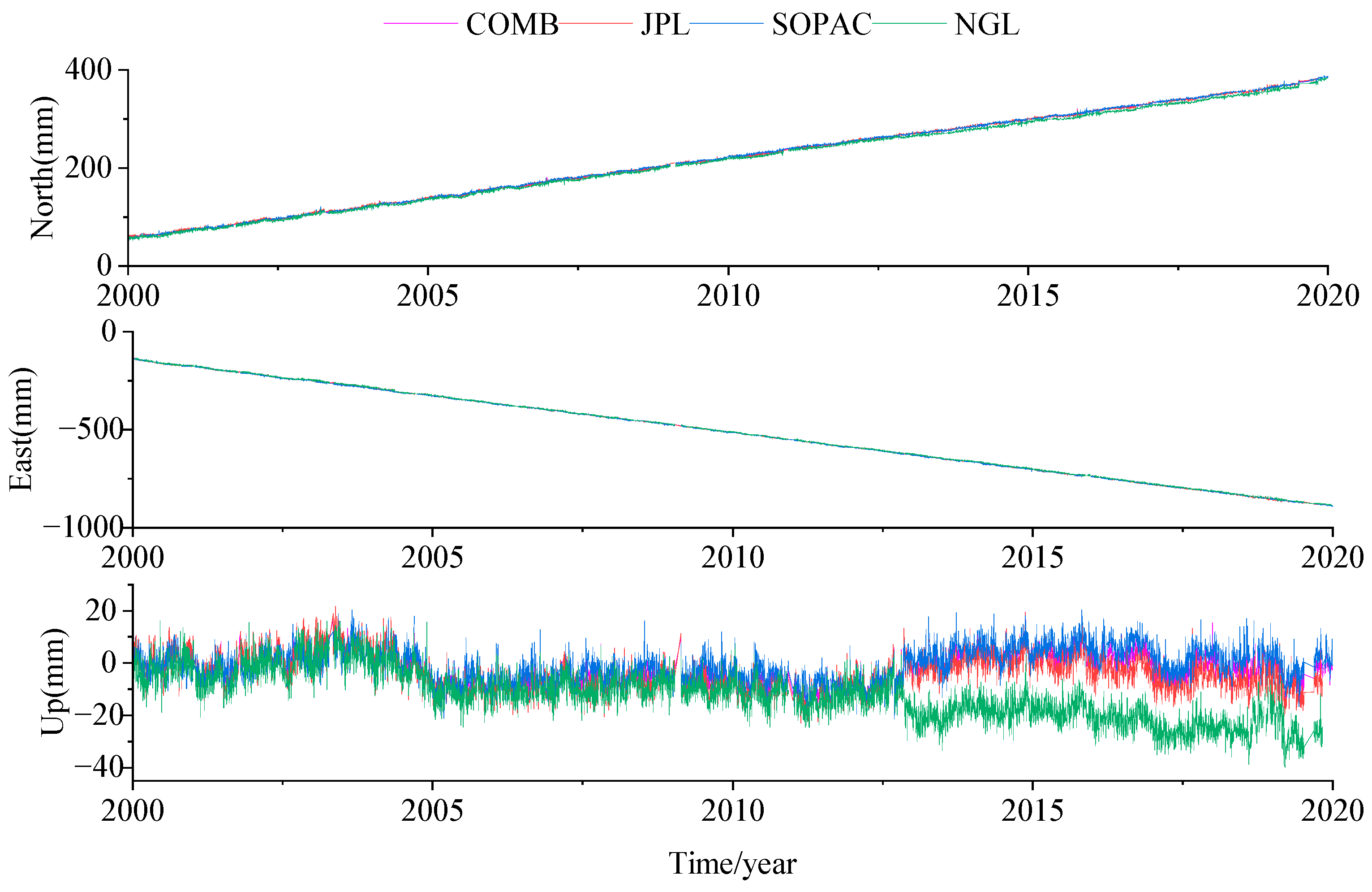
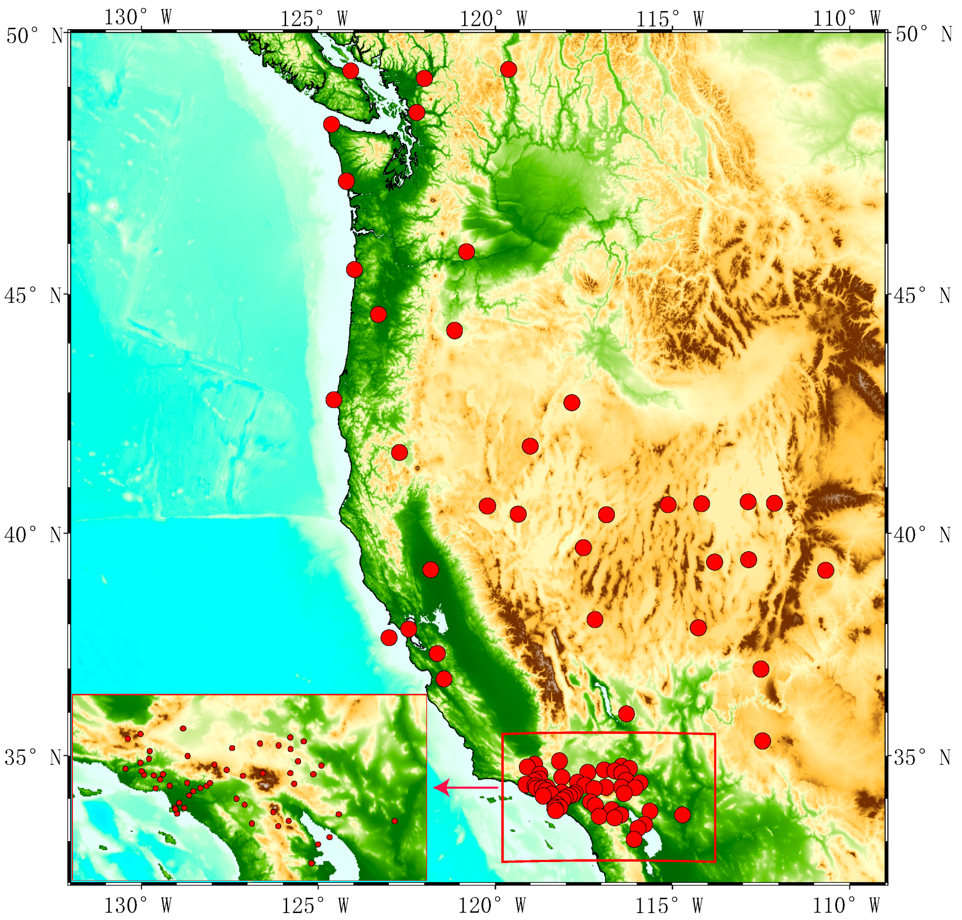
Recent studies have shown that the duration of GNSS time series significantly influences noise models. For high-precision geophysical applications, time series longer than 10 years are recommended to mitigate noise effects [46]. We select data from 87 GNSS stations located on the U.S. West Coast spanning 20 years (2000–2020). The distribution of these stations is illustrated in Figure 2. Four data products exhibit an average data gap rate below 6%, with the maximum rate not exceeding 10%.

After applying the 3IQR method to remove outliers from the selected data, detrending was performed separately on the E, N, and U components, followed by calculating their RMS values. The RMS values derived from different strategies for analyzing the data exhibit strong consistency, with the average RMS in the E and N components remaining within 3 mm and the RMS in the U component staying below 6 mm. For the aforementioned data, after outlier removal, offsets were detected and corrected individually. The COMB, NGL, and JPL data exhibit a similar total number of offsets, approximately 700 each. In contrast, SOPAC has the smallest total number of offsets, with only 431, possibly due to its adoption of different analysis strategies.

3.2. Geophysical Fluid Loading Effect on GNSS Time Series

GNSS time series exhibit significant seasonal variations, such as annual and semi-annual signals. The global periodic migration of surface loads causes mass redistribution, leading to surface changes. The influence of surface environmental loading introduces biases in the estimation of station displacements and velocities. To enhance the accuracy and reliability of the GNSS coordinate time series, load corrections are required to eliminate the non-tectonic movement variations induced by surface loading.

This study computed the Pearson correlation coefficients [47] to quantify the relationship between the sum of the non-tidal atmospheric loading (NTAL), non-tidal oceanic loading (NTOL), hydrological loading (HYDL), and GNSS time series from different analysis strategies. The correlation coefficients between the sum of loading components and the E component are approximately 0.65 for all four datasets. In the N and U components, the correlation coefficients are approximately 0.4. This indicates a correlation between the environmental loading series and GNSS time series, implying that the environmental loading series chosen in this study can be used to correct mass loading effects.

Table 2. Statistics for time series with reduced RMS values after loading correction.

Solutions	E	N	U	Mean
COMB	71.3%	83.9%	77.0%	77.40%
JPL	95.4%	98.9%	42.5%	78.93%
SOPAC	43.7%	26.4%	95.4%	55.17%
NGL	95.4%	96.6%	97.7%	96.57%

demonstrates significant changes in RMS values [48] before and after environmental loading correction. For the COMB and NGL datasets, over 70% of data in the E, N, and U components exhibit reduced RMS values post-correction. Environmental loading primarily affects the E and N components of JPL data, with over 90% of time series showing reduced RMS values, while the U component exhibits a reduction in RMS values for 42% of its time series. In the SOPAC data, 90% of the U component exhibits reduced RMS values, whereas less than 50% of the E and N components show reduced RMS values.

The impact of environmental loading on RMS values was further investigated by calculating the changes in RMS values after applying loading corrections across different datasets. As can be seen in

Table 3. Mean RMS variations after loading correction based on different analysis strategies.

Solutions	E	N	U	Mean
COMB	−1.50%	−5.60%	−5.00%	−4.03%
JPL	−3.70%	−8.30%	0.00%	−4.00%
SOPAC	0.50%	1.40%	−8.70%	−2.27%
NGL	−4.20%	−6.90%	−9.70%	−6.93%

, following loading correction, the RMS values for the E and N components of the SOPAC data and the U component of the JPL data showed minimal changes, while the RMS values decreased by approximately 5% for the other components.

In summary, there is a high correlation between HYDL, NTAL, NTOL, and data from different analysis strategies, implying that the environmental loading series chosen in this study can be used to correct mass loading effects. After loading correction, the RMS values for the majority of time series in these four datasets typically decrease by around 5%.

3.3. CME Effect on GNSS Time Series

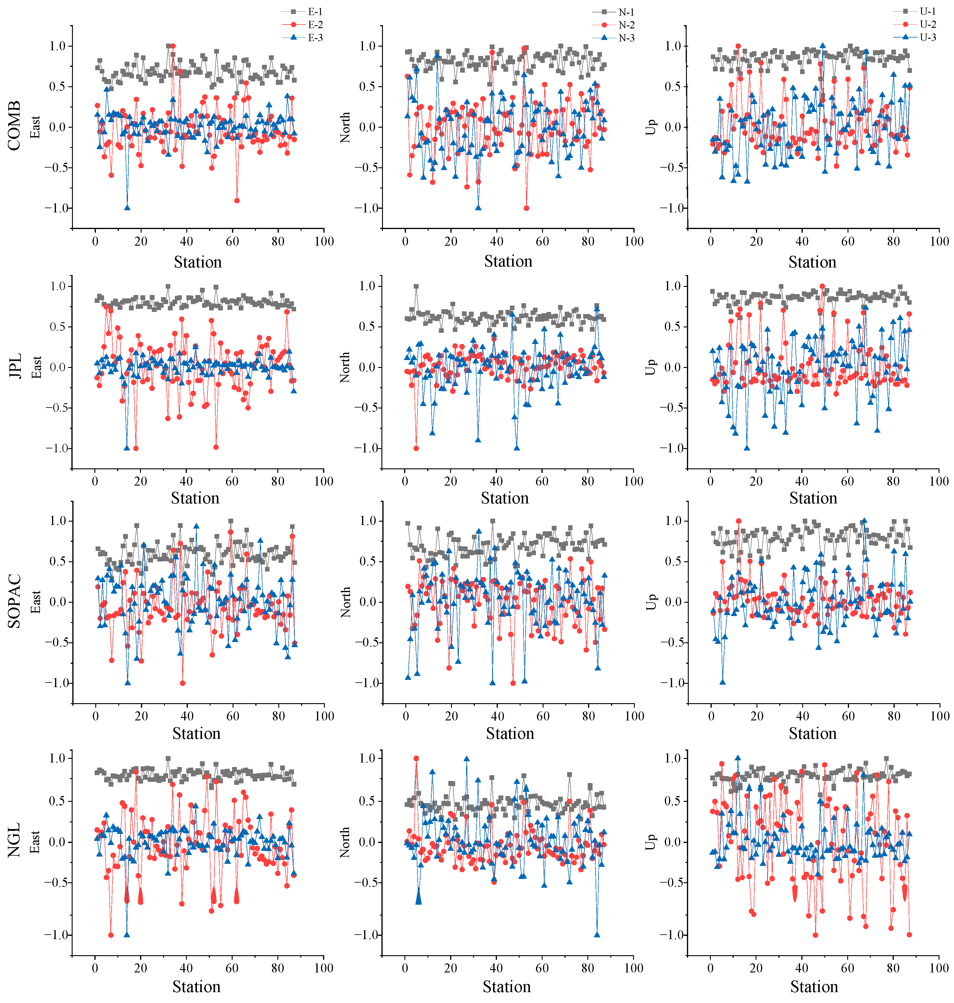
Before performing PCA filtering, we used the Regularized Expectation Maximization (RegEM) method to interpolate the GNSS time series [49]. This approach accounts for the correlation and physical context of the stations, requiring no prior information or reliance on external data models. Instead, it relies solely on the intrinsic characteristics of the data. Dong et al. [26] defined CMEs as follows: if a principal component (PC) shows significant standardized spatial responses (greater than 0.25) at most stations (more than 50%), and its eigenvalue exceeds 1% of the total sum of eigenvalues, it is considered to exhibit CMEs. Here, we determine the number of PCs with common mode errors based on the proportion of eigenvalues and standardized spatial responses. For the E, N, and U residual time series, filtering is conducted to obtain the percentage of total eigenvalues contributed by each principal component, as well as the standardized spatial responses of the first three PCs for each station’s coordinate time series. Standardized spatial responses are obtained by dividing each station’s spatial response by the maximum spatial response, where positive values indicate a positive spatial response to the principal component and negative values indicate a negative response. This can be seen in

Table 4. Contribution rates of the total eigenvalues of the PC of the residual series.

Solutions		PC1	PC2	PC3
COMB	E	45.55%	10.04%	5.00%
	N	38.85%	5.71%	4.83%
	U	38.12%	5.38%	3.82%
JPL	E	62.33%	4.61%	3.46%
	N	54.96%	6.61%	3.52%
	U	48.70%	5.53%	2.95%
SOPAC	E	46.75%	11.65%	4.86%
	N	43.06%	6.68%	6.18%
	U	37.12%	4.71%	4.14%
NGL	E	59.55%	6.50%	3.81%
	N	53.84%	9.75%	4.04%

and Figure 3 (ENU componments of the top 3 PCs).

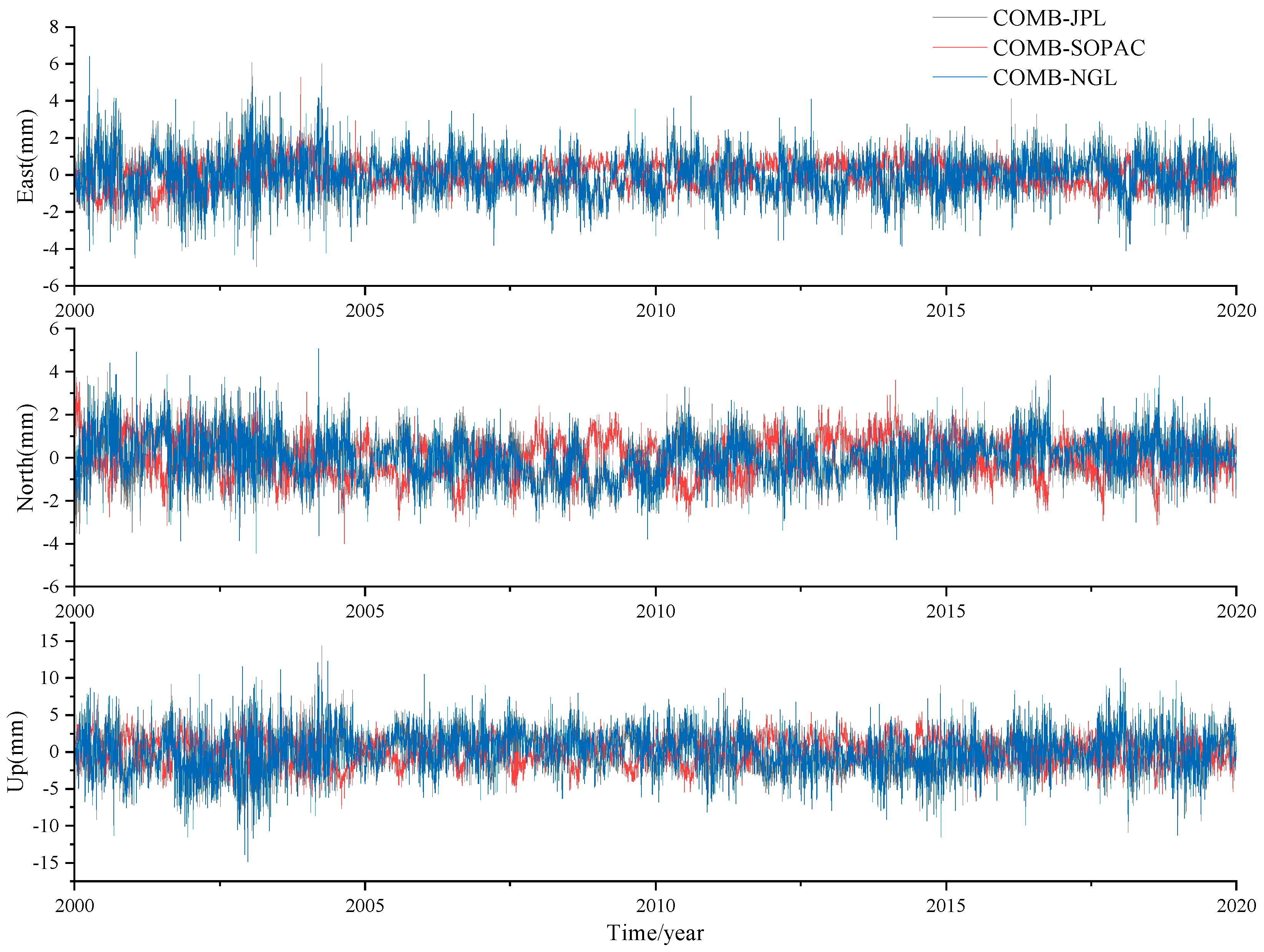
Figure 4 shows the CME difference for the E, N, and U components of the randomly selected CSN1 station in the time domain. The data from different analysis strategies show high consistency across all components, with differences below 5 mm in the E and N components and below 10 mm in the U component. Additionally, the RMS consistency of CME differences across various solution strategies demonstrates strong agreement, with RMS values below 1.5 mm in the E and N components and below 3 mm in the U component.

Further investigation into the relationship between CMEs and data analysis strategies involved computing the correlations between CMEs across different analysis strategies. As shown in

Table 5. CME correlation coefficients based on different analysis strategies.

Solutions	E	N	U
COMB-JPL	0.77	0.81	0.85
COMB-SOPAC	0.80	0.70	0.79
COMB-NGL	0.60	0.63	0.53

, there is a high correlation in CMEs between different solution strategies: COMB shows correlations around 0.8 with JPL and SOPAC and around 0.6 with NGL in various components. These findings suggest that CME is often present in GNSS time series, and its occurrence is independent of the data analysis strategy.

In the frequency domain, spectral analysis was used to detect periodic signals of CMEs across different datasets. Figure 5 depicts the power spectral density comparisons in the E, N, and U components for the randomly selected CSN1 station. The horizontal axis represents frequency, while the vertical axis represents power density. As shown in Figure 5, different data analysis strategies exhibit high consistency in the E, N, and U components, showing similar amplitudes of their periodic components. The most significant of these components is the annual term, indicating that CME is one of the primary causes of the seasonal fluctuations observed in GNSS time series.

Extracting and eliminating CMEs enhances the accuracy of regional continuous GNSS time series and deformation mode analysis. The removal of CMEs results in a decrease in the RMS values of all time series in the E, N, and U components across the four datasets. The average correction rate exceeds 20%, indicating that eliminating CMEs effectively reduces the errors in the model parameters of the time series, thereby enhancing the precision of the time series. The RMS values exhibit high consistency after CME removal; the RMS values for the E and N components are below 1.4 mm, while those for the U components are below 3.7 mm across all datasets.

In conclusion, the CME demonstrates a high degree of consistency among data derived from different analysis strategies in both the frequency and time domains, suggesting that the source of CMEs is independent of the data analysis strategy. After removing CMEs, the RMS values decrease across all four datasets with higher consistency, indicating that CMEs occur independently of the analysis strategy and may stem from large-scale atmospheric and hydrospheric effects, small-scale crustal deformations, or other unmodeled errors [3].

3.4. GNSS Time Series Noise Properties

Previous studies have shown that the noise in GNSS time series significantly impacts the uncertainty of station velocities, resulting in an underestimation when assuming a white noise background [25,50,51]. Overestimating the velocity accuracy in practical applications can lead to using unreliable data as reliable, which fails precision requirements and poses risks in high-precision GNSS applications. GNSS time series exhibit seasonal nonlinear variations, primarily due to uncorrected environmental loading and common mode errors. Correcting for nonlinear signals is essential to obtain the optimal noise model and achieve unbiased estimations of station velocities for time series. Therefore, this study examines the impact of data processing models and analysis strategies on noise characteristics in GNSS coordinate time series by evaluating four noise models: Flicker Noise + White Noise (FN+WN), Generalized Gauss–Markov Noise + White Noise (GGM +WN), Power Law Noise + White Noise (PL+WN), and Random Walk Noise + Flicker Noise + White Noise (RW+FN+WN). This study employs an enhanced Bayesian Information Criterion (BIC_tp) to analyze the noise characteristics of the different time series following load correction and common mode error removal.

Table 6. The optimal model for the ENU components derived from different analysis strategies.

Solutions		FNWN	GGMWN	PLWN	RWFNWN
E	COMB	33.3%	0.0%	50.6%	16.1%
	JPL	24.2%	0.0%	67.8%	8.0%
	SOPAC	26.5%	0.0%	56.3%	17.2%
	NGL	29.9%	0.0%	47.1%	23.0%
N	COMB	40.3%	1.1%	44.8%	13.8%
	JPL	24.1%	1.1%	65.5%	9.3%
	SOPAC	24.1%	0.0%	55.2%	20.7%
	NGL	20.8%	1.1%	60.9%	17.2%
U	COMB	25.4%	1.1%	67.8%	5.7%
	JPL	2.4%	1.1%	93.1%	3.4%
	SOPAC	52.9%	0.0%	19.5%	27.6%
	NGL	42.6%	2.3%	17.2%	37.9%

presents the distribution of optimal models in the E, N, and U components for the data derived from different analysis strategies. In the E and N components, the noise characteristics are generally similar across different datasets. COMB, SOPAC, and NGL exhibit high consistency, with the PL+WN and FN+WN models collectively accounting for approximately 80% of the total, while the RW+FN+WN model accounts for about 20%. In contrast, JPL shows significantly higher proportions of the PL+WN and FN+WN models, totaling up to 90%, while the RW+FN+WN model constitutes less than 10% compared with the other datasets.

Significant differences in noise characteristics are observed between the U component and the E and N components of the data. For the COMB data, there is a decrease in the proportion of the FN+WN and RW+FN+WN models, while the proportion of the PL+WN model increases, with the RW+FN+WN model accounting for only 5.7%. Over 90% of the time series in the JPL data are described by the PL+WN model. The SOPAC and NGL data show a shift in the predominant noise model from PL+WN to FN+WN, accounting for 52.9% and 42.5%, respectively. Moreover, a significant presence of random walk noise was detected in the U component, leading to a substantial increase in the proportion of RW+FN+WN models compared with horizontal components, accounting for 27.6% and 37.9%, respectively.

The diversity and complexity of GNSS noise confirm the presence of both white noise and colored noise in GNSS coordinate time series, meaning that a single noise model is insufficient to accurately describe them. At most stations, the horizontal components show higher consistency in noise models, while vertical components exhibit significant differences among datasets. Hence, in the pursuit of physical explanations for time series variations, it is essential to treat each component differently. The SOPAC and NGL data exhibit substantial RW noise components in various components, with over 20% of time series favoring the RW+FW+NN model as the optimal noise model. Meanwhile, the COMB and JPL datasets predominantly exhibit RW noise in the horizontal component, with RW+FW+NN models accounting for 8–20% of the noise models. This phenomenon may arise from the selection of time series spanning longer time periods, enabling accurate identification of challenging RW noise. The SOPAC and NGL data demonstrate a higher prevalence of RW noise, which can potentially be attributed to variations in data analysis strategies.

This study further explores the impact of different data analysis strategies on noise characteristics by comparing the consistency of the optimal models between COMB and other datasets. As shown in

Table 7. Consistency in noise models between comb and other analysis strategies.

Solutions	FNWN	GGMWN	PLWN	RWFNWN	Total
COMB_JPL	14	2	116	17	149 (57.09%)
COMB_SOPAC	34	1	66	24	125 (47.89%)
COMG_NGL	28	1	65	27	118 (46.36%)

, the noise characteristics of data from different analysis strategies demonstrate a high consistency, with the optimal noise models including COMB/JPL, COMB/SOPAC, and COMB/NGL for approximately 50% of the datasets. However, there are still instances of inconsistency in the noise models, indicating that the analysis strategies have an impact on the noise characteristics of the GNSS time series. Therefore, when conducting an unbiased estimation of noise models, it is crucial to consider the noise variations resulting from different analysis strategies and data processing models.

3.5. GNSS Time Series Velocity Analysis

Previous works [52,53] show that the International Terrestrial Reference Frame (ITRF) must achieve an accuracy of 0.1 mm/year when providing site coordinates in order to fulfill the stringent requirements of high-precision scientific applications. The determination of station positions and velocities with high accuracy is essential for high-precision GNSS time series applications, offering substantial theoretical and practical value. In this section, within the context of colored noise, we employ the optimal model selected in Section 3.4 to estimate velocities and their uncertainties from various analysis strategies. We have previously investigated the impact of different analysis strategies on site velocities and their uncertainties by calculating the differences between the COMB and data derived from the JPL, NGL, and SOPAC. Based on the statistical findings presented in Figure 6, it is observed that a significant majority of stations (80%) exhibit velocity differences below 0.3 mm/year and velocity uncertainty differences below 0.1 mm/year. However, a minority of stations demonstrate velocity differences exceeding 0.5 mm/year, indicating significant deviations in velocity and uncertainty estimates due to varying analysis strategies.

In summary, the analysis strategy and data processing model significantly influence the observed velocities and their uncertainties at stations. In high-precision GNSS applications, overlooking the impact of the analysis strategy can lead to biased estimates of station velocities, thereby posing risks to accuracy and reliability.

3.6. Periodic Signal Analysis of GNSS Time Series

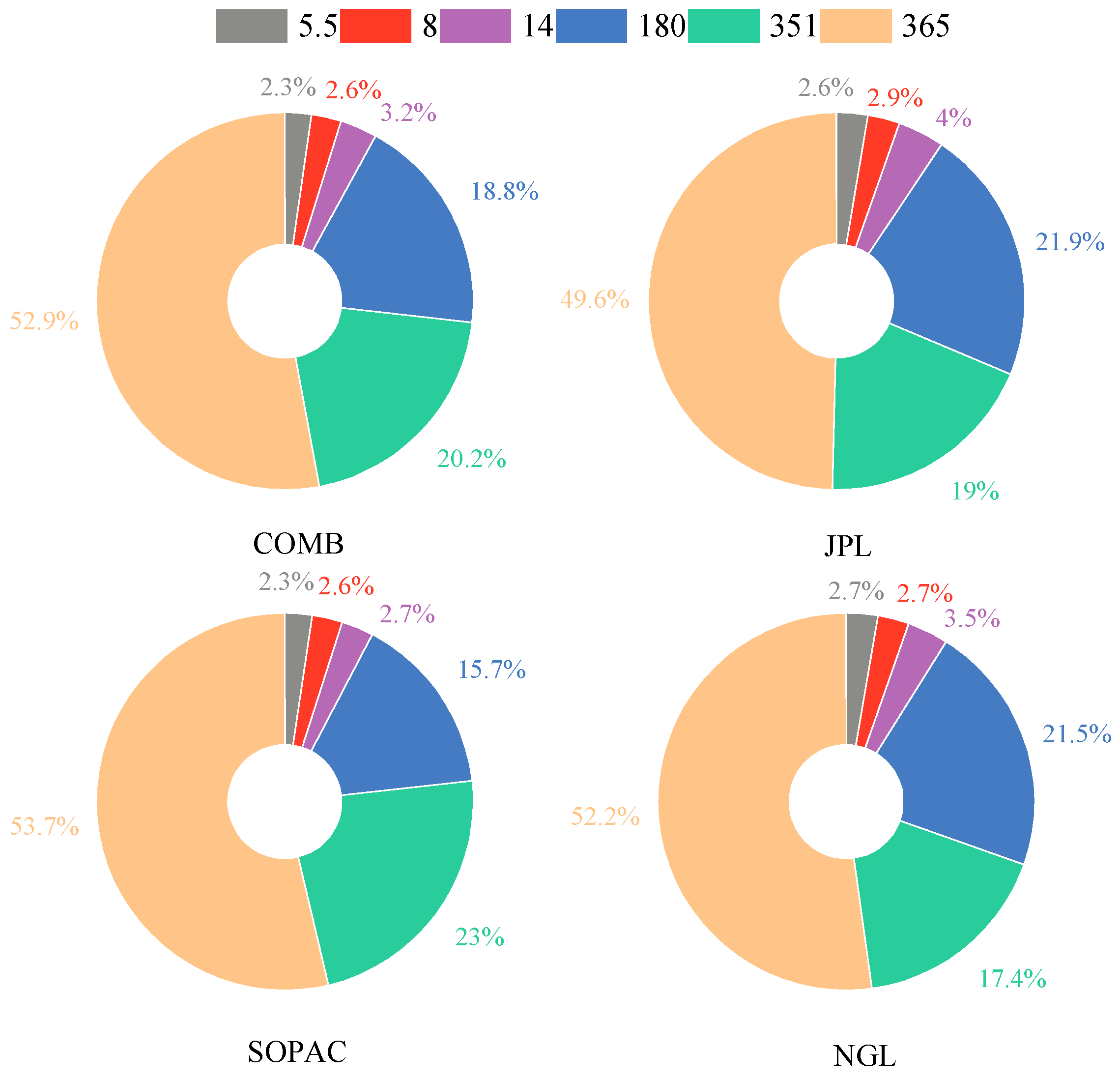
GNSS time series contain numerous periodic non-tectonic signals. Existing research has confirmed the presence of periodic signals with durations of 365, 351, 180, 14, 8, and 5.5 days [21,22,23,34,35]. The amplitudes of these periodic signals were calculated from the raw data according to their optimal noise model, and their average amplitudes were normalized to explore the relationship between different periodic signals and analysis strategies. As shown in Figure 7, there is a high degree of consistency in the normalized average amplitudes of different periodic signals across various analysis strategy datasets. The annual, semi-annual, and draconitic year signals account for approximately 90% of the total amplitude, while the 5.5-, 8-, and 14-day signals only contribute a minor amplitude of about 10%.

The average amplitudes of the periodic signals are calculated from the corrected loading data (see Section 3.2) to examine their potential association with environmental loading.

Table 8. Mean amplitude variations of different periodic signals after load correction.

Solutions	365	180	351	14	8	5.5
COMB	−49.71%	−26.25%	11.01%	0.00%	−1.72%	0.77%
JPL	−30.56%	−24.57%	16.36%	−0.97%	0.00%	1.06%
SOPAC	−37.90%	−11.48%	3.61%	3.03%	−3.17%	−1.15%
NGL	−36.43%	−25.49%	11.14%	−10.99%	−5.80%	−1.37%

presents the statistical results of the average amplitude variation rates.

This study found that environmental loading has a significant and consistent impact on annual and semi-annual signals. After load correction, over 80% of the time series in the COMB, JPL, and NGL datasets show a decrease in the amplitudes of their annual and semi-annual signals, with correction rates of approximately −40% for the annual signal and −30% for the semi-annual signal. For SOPAC, 60% of the time series exhibit a decrease in amplitude, with annual and semi-annual signal correction rates of −37% and −11%, respectively. This suggests that environmental loading is a significant factor influencing annual and semi-annual signals, with SOPAC time series showing a decrease in the amplitudes for these signals in only 60% of cases, potentially due to the use of a different load model compared with other datasets. Therefore, the impact of different analysis strategies and processing models should be considered when performing environmental load corrections. After environmental load correction, 30% of the SOPAC time series show a decrease in the draconitic year signal amplitude, with a correction rate of 3.6%. In contrast, about 20% of the time series in the COMB, NGL, and JPL datasets exhibit a decrease in amplitude, with a correction rate of 20%. This suggests that environmental corrections are not the primary factor influencing the draconitic year error, further confirming that this signal may be a systematic error in the GNSS modelation.. For the 14-, 8-, and 5.5-day periods, around 50% of the datasets derived from different analysis strategies demonstrate a decrease in amplitude after load correction, with minimal change rates. This also indicates that environmental loading is not the main cause of these periodic signals. The 14-day signal is likely due to imperfect tidal load modeling and signal aliasing.

Following load correction and the removal of CMEs (see Section 3.3), the average amplitudes of these periodic signals were computed to investigate their potential correlation with the origins of the aforementioned signals. The corresponding average variation rates are presented in

Table 9. Mean amplitude variations of different periodic signals after load correction and removal of CMEs.

Solutions	365	180	351	14	8	5.5
COMB	−57.84%	−50.79%	−48.18%	−28.31%	−22.08%	−15.88%
JPL	−61.41%	−60.33%	−50.90%	−42.34%	−27.38%	−22.93%
SOPAC	−60.09%	−42.50%	−49.63%	−17.37%	−21.74%	−16.97%
NGL	−61.62%	−60.99%	−49.11%	−42.71%	−31.44%	−24.85%

.

After removing the CME, in addition to environmental load corrections, it was observed that approximately 90% of time series across different analysis strategy datasets exhibited a reduction in the amplitudes of their annual and semi-annual signals, with an average change rate of approximately −60%. This suggests that the annual and semi-annual signals observed in GNSS time series primarily arise from surface mass loading effects and CMEs. The application of appropriate load model corrections and spatial filtering effectively isolates these influences. Approximately 95% of the time series in the NGL and JPL datasets exhibited a reduction in the draconitic year signal amplitude, with a correction rate of about −50%. For SOPAC and COMB, 78.1% and 84.7% of the time series showed a decrease in draconitic year amplitude, with correction rates of −46.9% and −41.8%, respectively. This suggests that the draconitic year signal observed in most stations stems from CMEs, rather than station-specific errors or environmental loads being the primary sources of this phenomenon. In each of the four datasets, more than 80% of time series exhibit a reduction in amplitude for the 14-, 8-, and 5.5-day periodic signals. Specifically, the correction rates for the 14-day signal average around −30%, for the 8-day signal, they average approximately −25%, and for the 5.5-day signal, they average about −20%. The findings suggest that the 14-, 8-, and 5.5-day periodic signals arise from unmodeled CMEs, which can be effectively mitigated through spatial filtering.

Currently, the origin of the 5.5-day periodic signal remains uncertain. This section aims to further investigate whether the generation of this periodic signal is associated with the analysis strategy. We calculated the average amplitude of the 5.5-day periodic signal for different analysis strategies. The data processed using GipsyX showed an average amplitude of 0.07 mm. In contrast, data processed using GAMIT/GLOBK from SOPAC and their joint solution COMB exhibited average amplitudes of 0.06 mm and 0.05 mm, respectively. These results suggest that data processed with GipsyX exhibit higher average amplitudes of the 5.5-day signal compared with other datasets. This implies that the GipsyX processing software may induce the 5.5-day periodic signal in GNSS time series.

Table 10. Amplitude distribution of 5.5-day raw data derived from different analysis strategies.

Solutions	<0.1 mm	0.1 mm~0.2 mm	<0.2 mm
JPL	75.1%	22.6%	2.3%
NGL	72.4%	24.9%	5.0%
SOPAC	88.1%	11.9%	0.0%
COMB	91.6%	8.4%	0.0%

presents the distribution of amplitudes for the 5.5-day periodic signal in the original time series. It is evident that approximately 70% of the data processed using GipsyX have amplitudes below 0.1 mm, with 5% of time series exhibiting amplitudes exceeding 0.2 mm. In contrast, for data processed using GAMIT/GLOBK from the SOPAC and their joint solution COMB, 90% of time series have amplitudes below 0.1 mm, and none of the time series have amplitudes exceeding 0.2 mm. These findings further corroborate that GipsyX processing software may contribute to the 5.5-day periodic amplitude in the signals.

We investigated this result by computing the average amplitudes of the 5.5-day periodic signal from the raw data, the environmentally corrected data, and the PCA-filtered time series. The statistical results are summarized in

Table 11. Average amplitude of 5.5-day signals based on different solution strategies (raw, load correction, and removal of CMEs).

Solutions	Analysis Software	Raw Amplitude (mm)	Loaded Amplitude (mm)	Pca Amplitude (mm)
JPL	GipsyX 2.1	0.07	0.07	0.05
NGL		0.07	0.07	0.05
SOPAC	GAMIT/GLOBK 10.71	0.06	0.06	0.05
COMB	Combine Solution	0.05	0.05	0.04

. Following PCA filtering, the average amplitudes of the 5.5-day signal that was obtained using JPL and NGL data processed with GipsyX remained higher than those obtained using SOPAC data processed with GAMIT/GLOBK and their combined solution COMB. This indicates that the use of GipsyX results in higher 5.5-day periodic amplitudes compared with GAMIT/GLOBK [54].

4. Discussion

In this paper, we showed that the consistency of stochastic noise properties is crucial for accurately estimating GNSS stations’ velocities, as the choice of noise model directly affects the velocity estimates. Using different analysis strategies, the optimal noise models are primarily PL+WN and FN+WN, though the occurrence of the RW+FN+WN model for the U component in JPL data is lower than in other datasets. This difference may stem from the fact that GAMIT employs a double-difference processing strategy, while GipsyX uses precise point positioning (PPP), although further investigation is needed to confirm the cause of this difference. Furthermore, the selection of GNSS stations and data centers is essential for the generalization of results. Therefore, future studies should incorporate more data centers and stations to evaluate the broader applicability of these conclusions and minimize the influence of biases on the result consistency.

The noise characteristics and periodic signal discrepancies warrant further investigation. These differences may result from environmental effects that have not been fully corrected or from intrinsic properties of the GNSS sites. By identifying the sources of these inconsistencies, future efforts are expected to enhance the accuracy and consistency of velocity estimations, thereby offering more robust data support for the long-term monitoring of geophysical phenomena.

5. Conclusions

In this study, 20 years of continuous observations of 87 GNSS stations were analyzed. GNSS time series derived from different analysis strategies and software packages were used: JPL, NGL (PPP strategy), SOPAC (double-difference strategy), and COMB (combined solution from JPL and SOPAC). This paper begins by examining the consistency of the data quality and delves into the individual relationships between environmental loading time series, common mode errors, and data analysis strategies. Subsequently, we analyzed the influence of analysis strategies on the noise characteristics of GNSS time series under conditions of colored noise using the BIC_tp criterion. Our study also investigates the consistency in velocity and uncertainty across various analysis strategies. Finally, the paper explores how environmental loading, common mode errors, and data analysis strategies impact periodic signals in GNSS time series. We can then conclude the following:

(1). This study demonstrates high consistency in both noise characteristics and velocity estimation across data from different analysis strategies. After correction for environmental loading and removal of CMEs, 50% consistency is observed in the optimal noise models. The velocity differences between datasets for 80% of the stations were below 0.3 mm/year, while approximately 10% of the stations exhibited velocity differences exceeding 0.5 mm/year, failing to meet the expected accuracy.

(2). This study revealed that the CMEs in the frequency and time domains exhibited high consistency across different analysis strategies. In the frequency domain, the CME showed consistent periodic components, notably the annual component. In the time domain, the RMS differences in CMEs between different analysis strategy datasets were highly consistent, with the differences in RMS values in the E and N components being below 1.5 mm and below 3 mm in the U component. This suggests that CMEs are prevalent in GNSS time series and are independent of the data analysis strategy.

(3). Our work revealed that the average amplitude of the 5.5-day signal for the JPL and NGL (using GipsyX 2.1) datasets was 0.07 mm, while for the SOPAC (using GAMIT/GLOBK 10.71) and COMB (combined solution), the average amplitudes were 0.06 mm and 0.05 mm, respectively. For the SOPAC and COMB datasets, 90% of time series had amplitudes below 0.1 mm, with maximum values not exceeding 0.2 mm. In contrast, for the JPL and NGL datasets, only 70% of time series had amplitudes below 0.1 mm, and 2.3% and 5% of time series, respectively, had amplitudes exceeding 0.2 mm. This indicates that the use of GipsyX results in higher 5.5-day periodic amplitudes compared with GAMIT/GLOBK.