Python Software Tool for Diagnostics of the Global Navigation Satellite System Station (PS-NETM)–Reviewing the New Global Navigation Satellite System Time Series Analysis Tool

Abstract

The time series of GNSS coordinates contain signals caused by the age-related movement of tectonic plates, the deformation of the Earth’s surface, as well as errors at different time scales from sub-daily tidal deformation to the long-term deformation of the surface load. Depending on the nature of the signal, specific approaches are used for both the visual interpretation and pre-processing of time series and their statistical analysis. However, none of the present software analyzes the nature of the residual errors but assumes their random nature and obedience to the classical normal distribution. One of the methods for analyzing the time series of coordinates with residual, unaccounted-for systematic errors is the non-classical error theory of measurements. The result of this work is a developed software solution for analyzing the time series of GNSS coordinates to test their normality, or in other words, to test whether a particular GNSS station is subject to the influence of small, unaccounted-for errors. Conclusions: After testing our software on four reference stations in Europe, we concluded that none of the chosen stations followed the normal law of distribution; thus, it is vital to perform such tests before conducting any experiments on the time series from reference stations.

1. Introduction

Continuous GNSS measurements provide scientists with a time series of coordinate changes not only to detect tectonic signals (lithospheric plate movement, geocentric movement, accumulation of crustal deformation, etc.) but also to respond to temporal variations in the surface load from various sources, such as tidal loading, atmospheric pressure, surface water, etc., as well as systematic errors that have not been fully modeled, including the erroneous modeling of satellite orbits, corrections for the phase center of the satellite/s and receiver antennas, multipath effects, etc. [1]. Both global/regional surface load responses and under-modeled errors lead to the spatial and temporal coherence characteristics of GNSS measurements over a fairly large area. It is known that such coherent characteristics are usually called Common Mode Errors (CMEs), which are the main spatially correlated signals in GNSS measurements [2]. The interaction between surface loading errors and spatial correlation errors can distort the station velocity estimate, increase velocity uncertainty, and even lead to incorrect geophysical interpretation. In order to improve the GNSS signal-to-noise ratio, it is highly recommended to apply various mathematical methods of CME filtering (stacking, reference frame transformation, and statistical signal decomposition techniques) [3,4,5,6]. It should be noted that the results of applying the stacking method directly depend on the size of the station networks and the distances between them. The results are satisfactory only if the CME in the regional network is essentially a spatially homogeneous medium. Accordingly, the assumption of equivalent CMEs for all stations in the network, even by introducing appropriate weights, does not solve the problem of identifying stations with strong local effects that may affect the detection of CMEs by this method. A similar situation exists in the case of transforming GNSS solutions into a regional reference system, i.e., stations located at the edge of the region may show distorted signals or some residual CMEs if they are affected by specific local effects. To mitigate the impact of CMEs, statistical signal decomposition techniques are also used. Among them, the most widely used ones are principal component analysis (PCA) [3], multi-channel singular spectrum analysis (MSSA) [5], and independent component analysis (ICA) [4], as well as their numerous modifications and evaluations. Based on the allowable heterogeneous distribution of CMEs (when a CME has only one source) and a more rigorous mathematical structure, these methods have been widely used to remove CMEs from the regional network. The main problem with these methods is the assumption that the residual errors of the GNSS coordinate time series obey a normal distribution law, known as Gaussian law, i.e., the mean and standard deviation are the best estimates used to find the true values and their errors. In the case of a long-term time series from individual GNSS stations, they might contain weak, unaccounted systematic errors [7,8]. They contribute to the deterioration of the accuracy of the station coordinates, the values of change rates obtained on their basis, as well as the concealment of many weak and transient signals in the coordinate time series (for example, the movement of neighboring faults). The estimation and removal of residual errors are performed using a number of classical statistical analysis methods, such as spatio-temporal filtering, the least squares method (LSM), and maximum likelihood estimation (MLE), which are implemented in all known software packages used for the analysis of the time series of coordinates [9,10,11,12]. In the EPN network, thresholds based on three different categories are used to select the most stable stations: positioning and signal quality, the reliability of determining the rate of change in coordinates, and station stability over the years.

The idea behind this selection is to discard the stations with the worst performance in each criterion. However, most of the classical methods of statistical analysis and EPN performance are based on the approach of the normal law of measurement error distribution, which a priori does not assume the presence of minor residual errors of a systematic nature that are not taken into account by models, for example, the tropospheric correction model [13]. The main purpose of this article is an attempt to identify the presence or absence of residual errors of a systematic nature at a single observation station based on the theoretical foundations of a non-classical approach to the statistical analysis of a long time series. To analyze the presence of residual unaccounted-for systematic errors at a particular GNSS station, the authors propose new software that can confirm or reject the hypothesis that residual errors follow the normal Gaussian distribution law, i.e., perform diagnostic mathematical modeling. This paper presents an overview of the non-classical method of geodetic time series analysis (Section 2), describes the process of using the Python v.3.9 software environment to develop a new software package for analyzing GNSS coordinate time series (Section 3), and evaluates the positioning of some stations in the EPN/IGS network using the developed GNSS software (Section 4).

2. Materials and Methods

2.1. Processing Time Series from Various Software

Topocentric GNSS time series are affected by various sources of errors, which are caused mainly by the spatial constellation of satellites, the GNSS signal propagation environment, and tracking stations. Thus, the accuracy of ephemeris, satellite oscillation corrections, Earth rotation parameters, ionosphere and troposphere effects, station stability, the multipath effect, electromagnetic signal interference, etc., have a decisive impact on the quality of time series obtained from GNSS observations [14].

Software for processing GNSS observations is usually based on double difference observations (relative positioning) or on absolute resolution (precise point positioning—PPP solution). The first case is called network positioning, where the baselines between all observed stations are estimated simultaneously. The second strategy, precise point positioning, is presented as a way to individually and efficiently estimate the station coordinates directly relative to a global network of GNSS reference stations. PPP calculates “absolute” positions at any location relative to a specific reference frame based on undifferentiated observations determined by the orbits of GNSS satellites. The network and PPP approaches can be considered equivalent in terms of obtaining a time series of GNSS coordinates.

In both methods, coordinates are usually evaluated relative to the International Terrestrial Reference Frame, the latest version of which, ITRF2020, was released at the end of 2022. It is not widely used yet in software packages. Therefore, for the analysis in this article, we use the previous implementation, ITRF2014.

Examples of well-known software packages for precise GNSS positioning and time series generation that use one of the two strategies described above are Bernese, GAMIT, and GIPSY-OASIS/GipsyX. However, other well-known packages, such as NAPEOS v.0.9.0 (Navigation Package for Earth Orbiting Satellites), PANDA (Position and Navigation Data Analyst), EPOS (Earth Parameter and Orbit Software), and the more recent PRIDE PPP-AR v2.2 (precise point positioning with ambiguity resolution) [15] can also be used. More details about the analysis strategies and physical models used in time series processing can be found in [2,16].

It should be noted that a GNSS time series might contain various offsets due to geophysical sources (e.g., atmospheric tidal loading, earthquake responses, etc.) or non-geophysical sources, such as changes in antenna height, changes in dissimilar antenna types, phase center modeling errors, inconsistencies in reference frames between analysis centers, etc. [5]. The time series administrator is responsible for detecting significant offsets and setting new offset parameters [17].

Various analytical centers (global, regional, national, or research) provide daily estimates of the positions of GNSS observation stations ($X,Y,Z$) in the global terrestrial reference frame IGbXX/ITRFXXXX [18]. These coordinates are then transformed into more intuitive and physically meaningful horizontal and vertical displacements ($N,E,U$) at epoch $t_i$ relative to some initial station coordinates ($X_0,Y_0,Z_0$) and initial epoch $t_0$. Then, a separate component of the time series ($N,E or U$) at discrete epochs $t_i$ can be modeled as $y_i=a+b{t}_i+f\left(x\right)$. The residual time series is formed from the differences between the observed (O, e.g., $N_i$) and calculated ($C, \mathrm{e}.\mathrm{g}.,y_i)$ coordinates, which characterize the degree of consistency between the model and the real data. Such differences are traditionally associated with observation–calculation (O-C) differences. Residual time series can be cleaned and filtered, but they are usually de-trended by definition, as the slope is one of the parameters estimated. The diagnosis of residual time series is an important element in the identification of deviations from the parametric model, including any unaccounted ones caused by physical processes and modeling errors.

2.2. Fundamental Differences between Classical and Non-Classical Methods of Mathematical Modeling

Mathematical data processing in natural sciences, as well as existing software products used for this purpose, are developed on the basis of classical ideas about observation errors, as outlined in the works of the famous mathematician C. F. Gauss. Classical notions of errors mean, first of all, the normal nature of their distribution. Upon such conceptions of errors, the following most important hypotheses are equivalent: (a) the normal law is adequate to the actual distribution of observational errors; (b) the arithmetic mean is an effective estimate of the observed value; and (c) the root mean square error (RMSE) is an effective estimate of measurement accuracy. The fundamental condition that gives the right to use this method can be written as follows:

$$\frac{f^{\prime }\left(x_i\right)}{x_i·f\left(x_i\right)}=const$$

(1)

where $f\left(x_i\right)$ is the probability density of the observational errors, $x_i,$ in a given experiment.

If the normal law is inadequate to the real distribution of observational errors, this means that it is impossible to (a) use the arithmetic mean in the study; (b) use the RMSE as the assessment of the accuracy of observations or measurements; or (c) use the arithmetic mean standard deviation ${\sigma }_{\overline{x}}=\sigma /\sqrt{n}$ or build confidence intervals for it. The famous scientist G. Jeffreys [19] showed that when the number of repeated measurements is n < 500, Gauss’s law usually remains adequate. However, due to the sharp increase in the amount of measurement information (the era of large samples), the normality hypothesis is both practically and theoretically untenable. This has been noted by many researchers [20].

With comparatively small samples of 30 < n < 500, it is difficult to prove that the error distribution deviates significantly from Gauss’ law while criterion procedures are being used. But even now, when the amount of measurement information increases significantly, some researchers tend to believe that deviations from the Gaussian error model can be ignored. They consider that the statistical procedures that are optimal for the normal model are approximately the same in the case of deviations from this model.

For n > 500, the distribution of the observational errors can be satisfactorily represented by the Pearson–Jeffreys law:

$$f\left(x\right)=\frac{\mathsf{\Gamma }\left(m+1\right)}{\sqrt{2\pi \left(m-0.5\right)}·\mathsf{\Gamma }\left(m+0.5\right)}·\frac{1}{\sigma }·{\left[1+\frac{m^2}{2{\left(m-0.5\right)}^3}·{\left(\frac{x-\mathsf{\lambda }}{\sigma }\right)}^2\right]}^{-m}$$

(2)

where $\mathsf{\Gamma }$ is the Gamma function; $\lambda ,\sigma ,m$ are distribution parameters. In fact, Formula (2) is the generalization of the Gaussian and Student distributions; when $m=\infty$, it is the Gaussian distribution, and when $m<\infty$, it is Student’s distribution for discrete values of degrees of freedom: $\nu =2m-1$.

G. Jeffreys [19] concluded that if the measurement errors are perfectly random (the influence of systematic error variables in the results of observations can be neglected), then the parameter $m$ of the distribution (2) should be within the following range:

$$3<m<5$$

(3)

It is evident that these limits are very far from $m=\infty$, which corresponds to Gauss’s law in (2).

So, (a) in contrast to condition (1), the main important postulate of non-classical modeling methods is the following:

$$\frac{f^{\prime }\left(x_i\right)}{x_i·f\left(x_i\right)}\ne const$$

(4)

(a) Non-classical procedures allow the efficient estimates of mathematical model parameters to be obtained, even under condition (4); (b) the influence of weak, non-excludable-dependent systematic errors can be neglected only when the Pearson–Jeffreys law $m$ falls within the limits of (3).

In recent years, the ideas, approaches, and methods of NETM have been tested in various fields of research: astronomical, space, gravimetric, geophysical, geodetic, and others. Thus, in [20], a method of a posteriori control over the stability of observation conditions identified by modern absolute ballistic gravimeters of free fall acceleration based on the methods of the non-classical error theory was developed alongside a NETM diagnosis of the probabilistic form of measurement distributions to improve the methodology of these high-precision determinations.

2.3. Algorithm for Estimating the Accuracy of the Results of GNSS Measurements Identified by the Non-Classical Error Theory of Measurements

The essence of the theory of the mathematical diagnostics of models in GNSS time series is reduced to the statistical analysis of the differences in “observation–calculation” (O–C) based on the following weight function:

$$p\left(x_i\right)=\frac{f^{\prime }\left(x_i\right)}{x_i·f\left(x_i\right)}={\left[{\left(\frac{m-0.5}{m}\right)}^3·\sigma +\frac{x_i^2}{2m}\right]}^{-1}$$

(5)

which allows for a fairly rigorous, simple, and visual assessment of the modeling accuracy. Usually, the differences (O–C) are obtained as residuals of the time series.

The influence of weak, non-excludable correlated systematic errors can be neglected only if the weighting function of measurement errors (5) is non-singular. It should be noted that the weighting function is non-singular only if it is sufficiently proven that the actual distribution of errors corresponds to Formula (2). Weight function (5) is singular when the error distribution has significant asymmetry.

Let us consider the algorithm of actions for evaluating the results of high-precision GNSS observations, namely, modeling diagnostics using the NETM. The software package for diagnosing GNSS stations uses data of high-precision determinations of spatial topocentric rectangular coordinates ($N,E,U$) at permanent observation stations as part of international, regional, or national networks. It should be noted that their reliable accuracy should be at the level of several mm, and the errors in the rate of coordinate changes should not exceed 0.1–0.3 mm/year.

Therefore, the following algorithm for diagnosing time series modeling using mathematical methods of statistics and NETM is proposed below:

• Finding the arithmetic mean of sample n > 500;
• Calculating errors and central sampling points;
• Calculating the skewness ($A)$ and kurtosis ($\epsilon )$ of the sample using unbiased central moments $m_2-m_8$ [20]:

$$m_r=\frac{\sum {\left(x_i-\overline{x}\right)}^r}{n}$$

(6)

where $r=2, 3, 4, 5, 6, 8$; $\overline{x}=\frac{\sum x_i}{n}$;

4.

Finding the standard of skewness (${\sigma }_A)$ and kurtosis (${\sigma }_{\epsilon })$;

5.

Building confidence intervals for skewness and kurtosis. To diagnose the modeling, it is enough to find 90% confidence intervals, i.e., using the quantile $t_{\alpha }=1.645,\alpha =10\%$ , and the following formulas: $A\pm 1.645·{\sigma }_A,$  $\epsilon \pm 1.645·{\sigma }_{\epsilon }$. Provided that the confidence intervals for $A$ and $\epsilon$ cover zero, processing the GNSS observations can be limited to classical estimation methods;

6.

Performing diagnostics of mathematical modeling through «observation–calculation» differences based on the constructed confidence intervals for the skewness and kurtosis. NETM methods should be used when the confidence interval for ($H_0$:$A=0$) covers zero and when the entire interval for $\epsilon$ is in the positive region ($H_0$:$\epsilon >0$) or the confidence interval is in the negative region ($H_0$: $\epsilon <0$) without covering zero. All other cases indicate various pathologies in the operation of GNSS equipment, the processing, or unacceptable observation conditions (the state of the antenna installation center, the presence of a constant source of multipath signals, specific local geophysical parameters, etc.). All the diagnostic parameters based on the constructed confidence intervals for skewness and kurtosis can be found in

Table 1. Diagnostics of mathematical modeling by residual errors.

Result	Diagnosis by Result
Confirmation of hypotheses: $(H_0$$: A=0$$), (H_0$$: \epsilon =0$)	There is no need to apply NETM.
Confirmation of hypotheses: $(H_0$$: A=0$$), (H_0$$: 1.2<\epsilon <6$) $(H_0$$: A=0$$), (H_0$$: 0<\epsilon <1.2$) $(H_0$$: A=0$$), (H_0$$: \epsilon <0$)	There is an effect of weak systematic errors that were not excluded when processing GNSS observations. An evaluation by NETM methods is required.
Confirmation of hypotheses: $(H_0$$: A<0$$) \mathrm{i} (H_0$$: \epsilon =0$) $(H_0$$: A>0$$) \mathrm{i} (H_0$$: \epsilon =0$) $(H_0$$: A<0$$) \mathrm{i} (H_0$$: \epsilon <0$) $(H_0$$: A>0$$) \mathrm{i} (H_0$$: \epsilon >0$) $(H_0$$: A<0$$) \mathrm{i} (H_0$$: \epsilon >0$) $(H_0$$: A>0$$) \mathrm{i} (H_0$$: \epsilon <0$)	Significant data pathology. Evaluation is not possible.

;

7.

Testing the null hypothesis $H_0$ for the law of distribution of the total sample (a measure of the approximation of the theoretical and empirical distributions) with the use of Pearson’s χ2 and Kolmogorov–Smirnov’s criteria ($D_n$ statistics) [21,22];

8.

Receiving a general conclusion about the accuracy assessment of GNSS observations using the NETM diagnostics.

3. Results

3.1. Program Language and Installation

The PS-NETM v.1.0 software tool was developed in Python, version 3.11. A number of libraries were used in the development of the software, as follows:

Pandas is a software library written for data manipulation and analysis (in particular, it offers data structures and operations for manipulating numerical tables and time series);

• Numpy is a library that adds support for large multidimensional arrays and matrices, along with a large library of high-level mathematical functions for operations on these arrays;
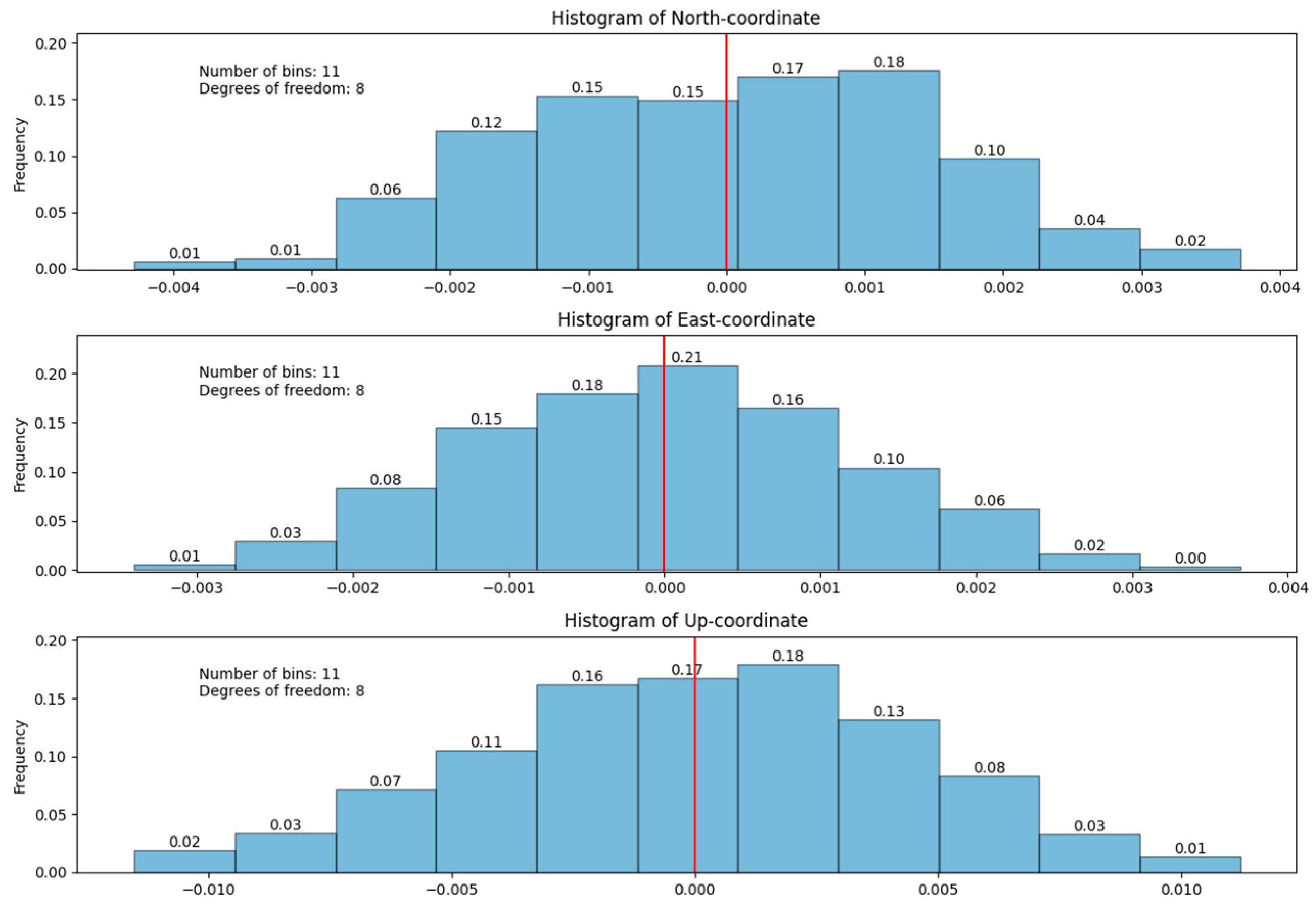
• Scipy is a library of high-quality scientific tools for the Python programming language (in particular, it is used to calculate the value of the Laplace function at the ends of histogram intervals and to calculate Pearson’s criterion (χ2));
• Matplotlib is a library whose main purpose is to visualize data with 2D graphics; it is used to create and draw error distribution histograms and time series graphs;
• Pywt is the implementation of wavelet analysis in Python; it is used to partially remove white and colored noise from the time series [23];
• PyEMD is the implementation of the Empirical Mode Decomposition filter in Python;
• PyQT is a Python shell for the Qt library. It was used to create a UI.

PS-NETM does not require any pre-installation by the user. The only requirement is Windows 10 or 11 (×64) and a Python interpreter on the system.

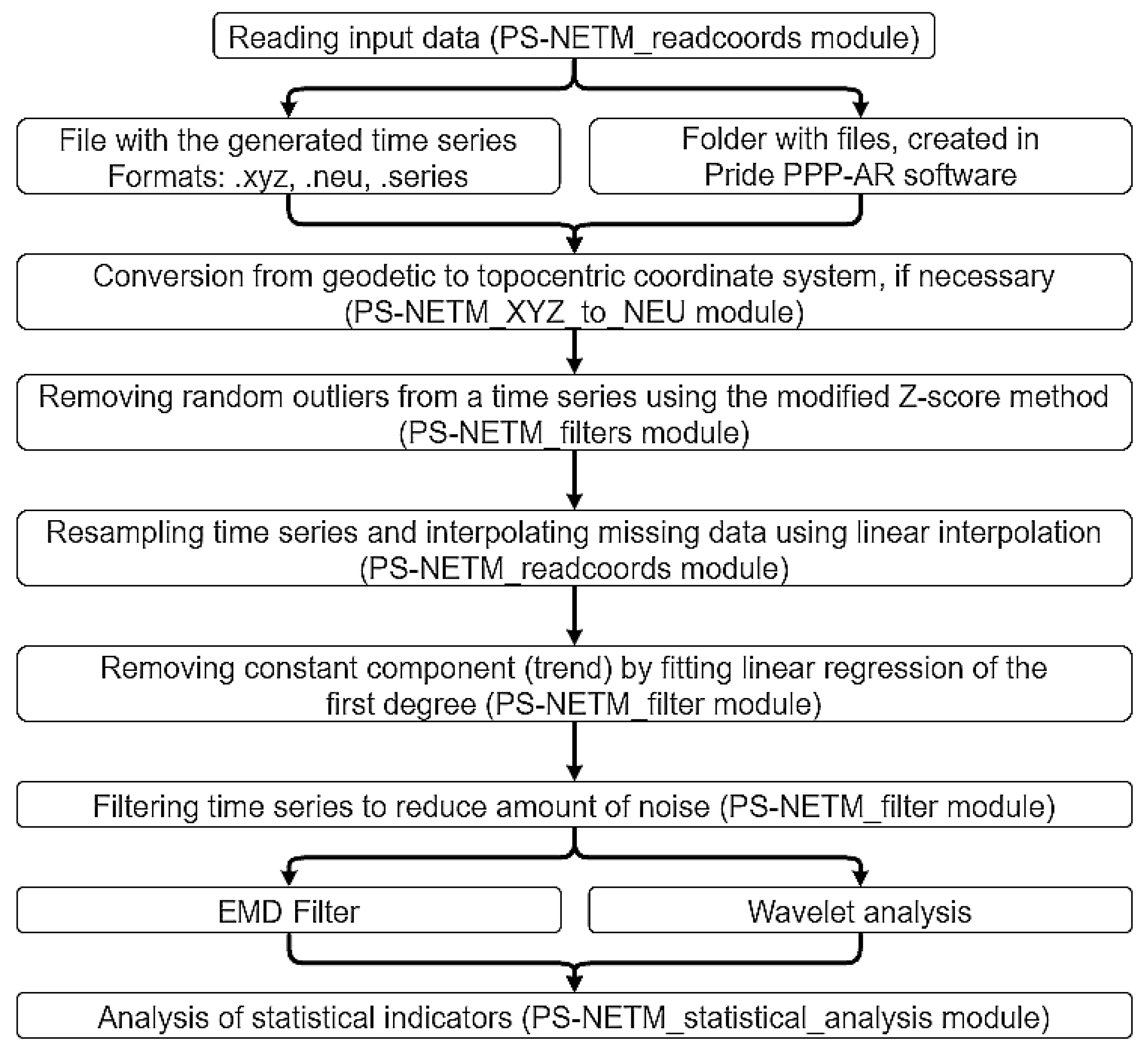
3.2. Structure of the PS-NETM Software

PS-NETM is a software product whose main purpose is the statistical analysis of time series of permanent GNSS station coordinates based on the use of mathematical methods of statistics and NETM.

Structurally, the PS-NETM software product consists of several modules. Figure 1 shows a brief description of each of them.

The first five modules (see Figure 1) are aimed at the preliminary processing of input data.

• Reading data from a specified file (if the time series has already been generated) or a folder with pos-files (PS-NETM_readcoords module);
• Converting from a geocentric to topocentric coordinate system if necessary (PS-NETM_XYZ_to_NEU module);
• Removing random outliers from the time series using the modified Z-score method (PS-NETM_filters module);
• Resampling the time series and interpolating missing data using the linear interpolation method. (PS-NETM_readcoords module);
• Removing the constant component (trend) by fitting linear regression of the first degree.

Once all five procedures have been performed, preprocessing is considered complete.

The next step is to filter the time series. PS-NETM supports the following two filtering methods: EMD (Empirical Mode Decomposition) filter and Wavelet analysis.

The EMD method is a signal decomposition method that was first proposed in [24]. It is a data-driven method that can decompose a nonlinear and nonstationary signal into a finite number of components called intrinsic mode functions (IMFs). EMD can adapt to the characteristics of the signal and reveal its underlying structure without any prior assumptions. EMD is a widely used method for reducing noise influence on GNSS time series; its main feature is that the filtering process is completely “unbiased”, meaning that no prior assumptions are made about its signal structure. For our software, we incorporated Ensemble EMD (EEMD), which is an improved version of EMD. It is more computationally expensive but mitigates the main drawback of a regular EMD, mode mixing, by adding white noise to the original signal before applying EMD.

Wavelet transformation is a mathematical tool that decomposes a signal into different frequency components and then studies each component with a resolution matched to its scale. Wavelet transformations are classified into two different types as follows: discrete wavelet transform (DWT), which uses a set of orthogonal wavelet basis functions (so-called “mother wavelets”), and continuous wavelet transform (CWT) which uses a continuous family of wavelet functions. In PS-NETM, two discrete wavelets are available as denoising options–Symlet4 and Coiflet5. Both of these wavelets are modifications of Daubechies wavelets, although they possess slightly different characteristics. While both wavelets are orthogonal, coiflets are designed to be asymmetrical, which is useful when dealing with different scales in signal [25]. Symlets, on the other hand, are near symmetrical, making them more appropriate for symmetric patterns of signal.

Other alternative filtering methods are least squares estimation (LSE), bandpass filtering, and low-pass filtering. LSE is one of the most widely used methods for noise filtering in GNSS time series due to its simplicity and computational efficiency. However, it assumes that the noise is Gaussian and independent, which is untrue in the case of a GNSS time series. Bandpass filtering is a technique that allows extracting signals of interest from a time series by removing the components that are outside a certain frequency range. Its main drawback is that it requires prior knowledge or estimation of the noise frequency band. Low-pass filtering is another simple and effective way to mitigate noise in time series by removing high-frequency noise components. This, however, may result in the attenuation of high-frequency components of the signal.

The last step of PS-NETM data processing is the calculation of statistical indicators required for analyzing the series using the non-classical theory. These indicators are the skewness ($A$), kurtosis ($E$), their errors (${\sigma }_A$ and ${\sigma }_E$), and confidence intervals ($cA$ and $cE$). Based on these indicators, PS-NETM concludes that the residual time series modeling is adequate, namely that the O-C differences should (or should not) ideally follow distribution (2) with the values of the $m$ index within (3).

In order to obtain correct statistical indicators, a number of requirements are imposed on the input data, namely,

• The number of measurements in time series should be at least 500 actual values, which, in the case of GNSS coordinate series, means daily station coordinates for a year and a half observation period;
• The number of missing observations should not exceed 5% of the total amount of data;
• PS-NETM is not recommended for analyzing stations in seismically active regions.

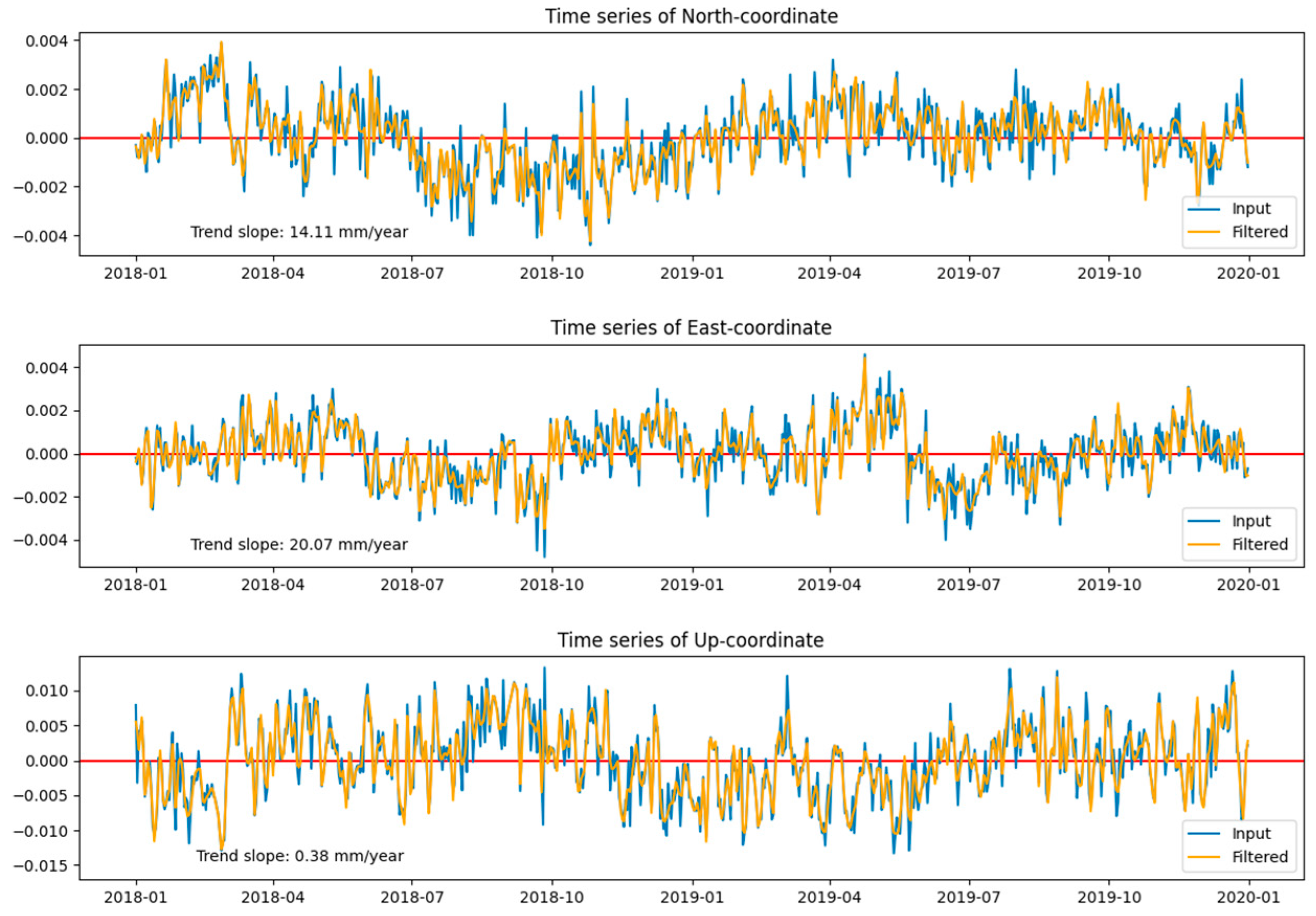
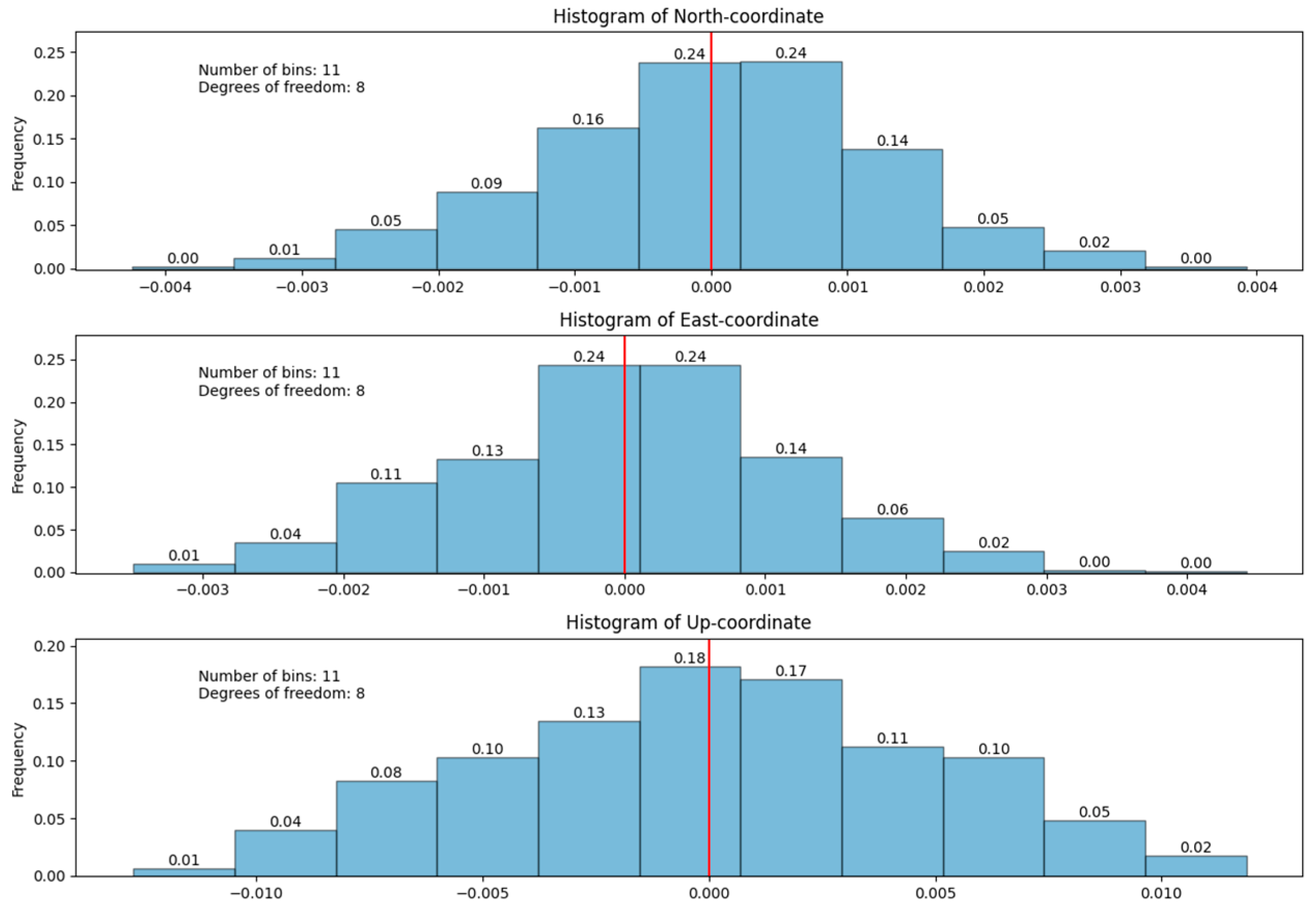
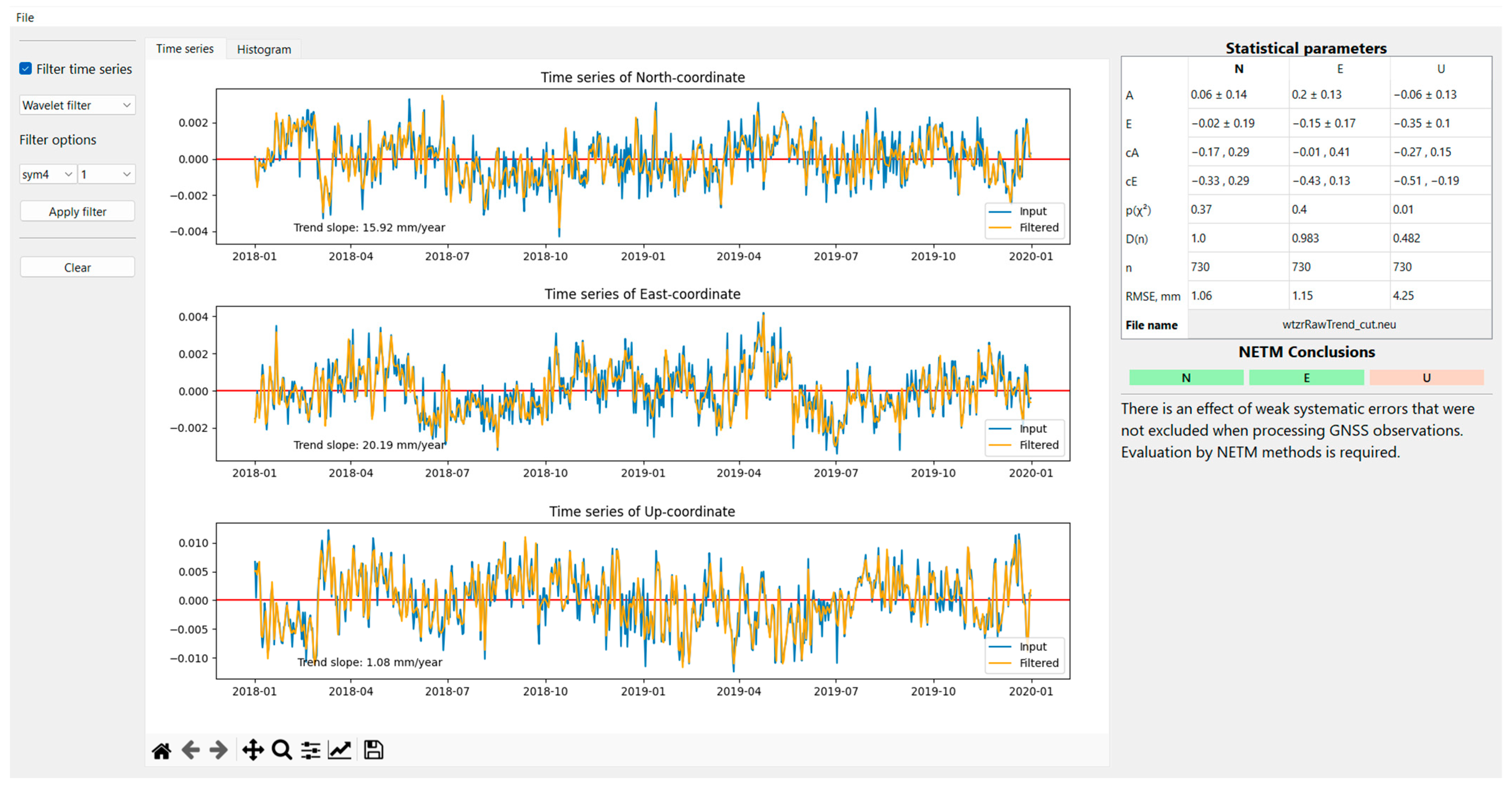
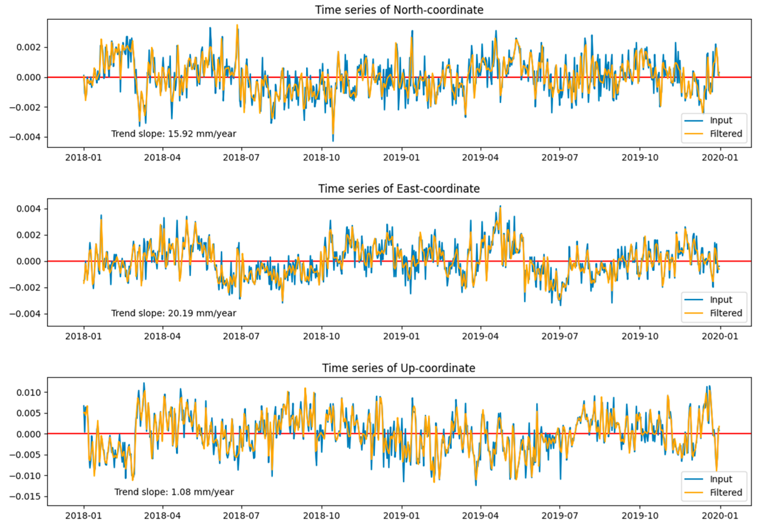
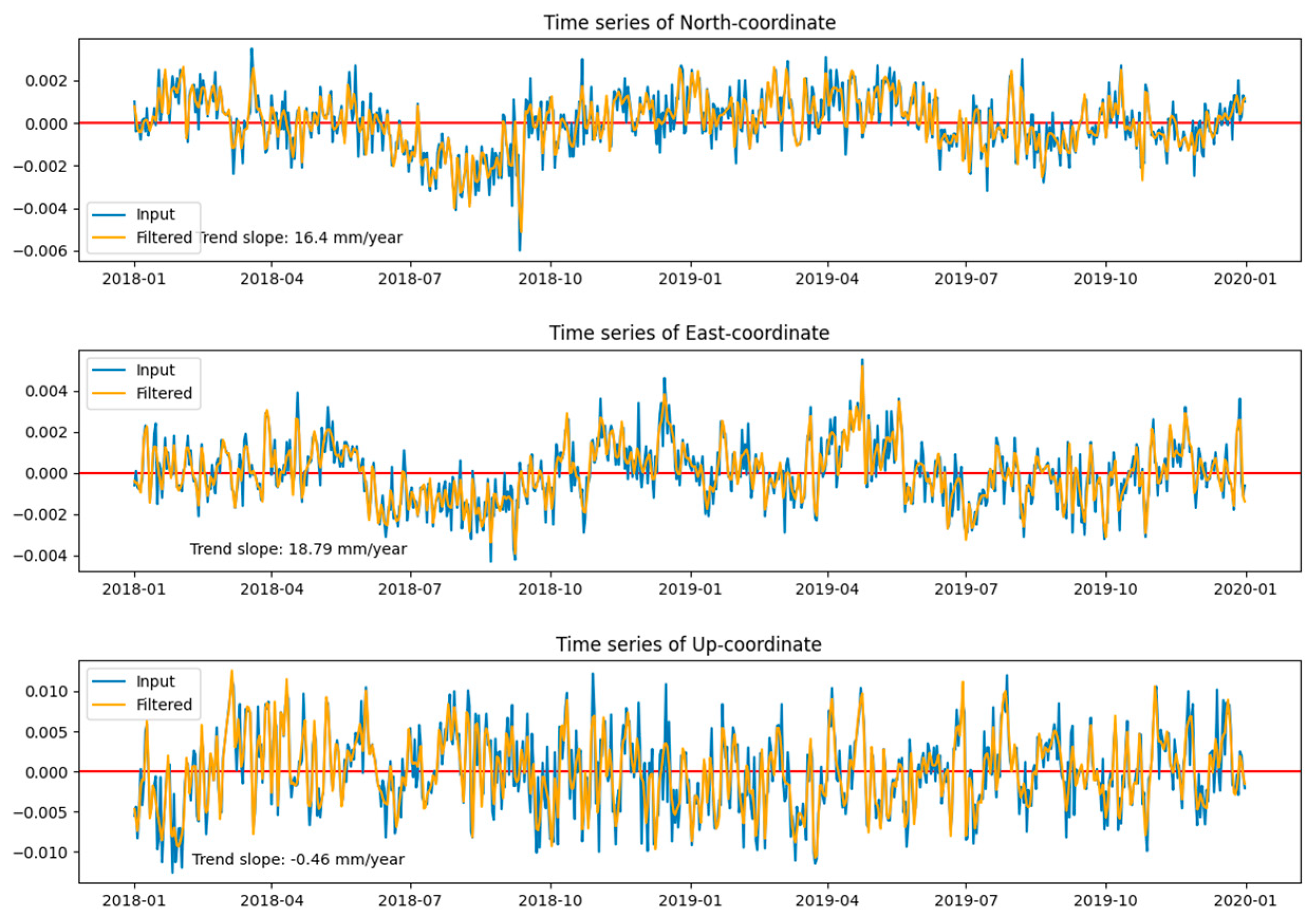
3.3. GNSS Position Time Series Conversion and Visualization in PS-NETM

Since time series are supplied by various data analysis centers in arbitrary formats, PS-NETM supports such formats as *.series, *.NEU, and *.XYZ.

It is also possible for users to create their own time series based on *.pos files made in Pride-PPPAR [15]. If you wish to manually create your own time series, PS-NETM can work with *_pos files created in PRIDE PPP-AR v.2.2 Software (also available at GPS Toolbox). In that case, the user is required to choose a folder that contains only pos-files generated with PRIDE PPP-AR. If any other files (or subfolders) are present in the chosen directory, the user is notified with an error message.

To start working with PS-NETM, the user needs to specify the path to the input data. Once the data are successfully adapted to the software environment, the interface displays time series plots (a time series tab) and histograms of the residual error distribution for each coordinate component N,E,U (Histogram tab).

The graphs for each coordinate show the trend parameters. On the right side of the screen, a table with statistical indicators and a conclusion about the series is located.

When the user applies the filter, the histogram, table, and conclusions are updated according to the “clean” data, and the graphs are supplemented (Figure 2).

The result of data processing in PS-NETM is the results table with time series statistics and NETM conclusions according to the NETM. A description of the results table is given in

Table 2. Description of the results table in PS-NETM.

A	Skewness of Dataset
E	Kurtosis of dataset
cA	Confidence interval for skewness
cE	Confidence interval for kurtosis
p(χ2)	Pierson’s chi-square criteria
D(n)	Kolmogorov–Smirnov criteria
n	Number of observations
RMSE, mm	Root mean square error
File name	Name of file (folder)

.

All these data can be exported for further processing. To export tabular data, the export conclusion function (file–export conclusion) is used. It should be noted that along with information that is present on screen, the ‘export’ option also writes the values of unbiased central sampling moments, which are used to calculate skewness and kurtosis (see Equation (6)) (Figure 3). If the export is successful, a corresponding message appears on the screen.

Also, during the processing, histograms of the residual error distribution with information about the number of degrees of freedom are created (Figure 4): $k=m-s$, where $m$ is the number of grouping intervals, and s is the number of superimposed connections. To visualize the generated histograms, it is enough to activate the Histogram tab.

As can be seen from Figure 4, a separate histogram is created for each individual coordinate, as they are individually analyzed by PS-NETM. Each bar has a relative frequency on top of it, depicting how many residual values it contains. The red line is used for a more comfortable visualization of distribution, as it clearly depicts whether it is the zero mean or not.

Based on the data obtained for the construction of histograms, the matching criteria are determined to test the null hypothesis that the empirical law of sample distribution obeys the theoretically predicted law of distribution of the population. Among the well-known K. Pearson, Kolmogorov–Smirnov, N. Kuiper, G. Watson statistical criteria of agreement, and Wilcoxon signed-rank test, etc., the first two were chosen. These criteria, in the authors’ opinion, are used in mathematical statistics most often.

3.4. Test and Results

To conduct the experiment, data were selected from four permanent GNSS stations that are simultaneously part of the IGS and EPN (EUREF Permanent GNSS Network) networks, namely, WTZR, HELG, PTBB, and WROC. This choice was made because the SOPAC [18] or CDDIS [26] databases contain the time series of these stations for the entire period of their operation, and the EPN website [27] provides information on their classification. The classification proposed there is aimed at identifying “stable” and “reliable” permanent stations and is based on the use of traditional mathematical apparatus.

The time series were formed with a daily frequency for the period from 1 January 2018, to 31 December 2019, so the final number of series was 730 days. At all stations, identical LEIAR25.R4/R3 antennas were installed, although the receivers were from different manufacturers.

Table 3. Characteristics of GNSS base stations.

Station Name	Location	Status in EPN
		Included Since	Class
WTZR	Wetzell/Germany	31-12-1995	C0
HELG	Helgoland Island/Germany	28-11-1999	C1
PTBB	Brauschweig/Germany	23-04-2000	C5
WROC	Wroclaw/Poland	24-11-1996	C6

shows some technical characteristics of the selected stations.

The data preparation procedure was the same for all stations: trend removal, the interpolation of missing data, and filtering. For filtering, the Symlet 4 Wavelet analysis of the first order was used. This filtering method reduced the amount of white noise and, at the same time, preserved the main properties of the signal. The results of the PS-NETM software are shown in

Table 4. Time series statistics for each of the selected stations.

Station		RMSE, mm	Asymmetry and Its Deviations	Confidence Interval for A	Kurtosis and Its Deviation	Confidence Interval for E
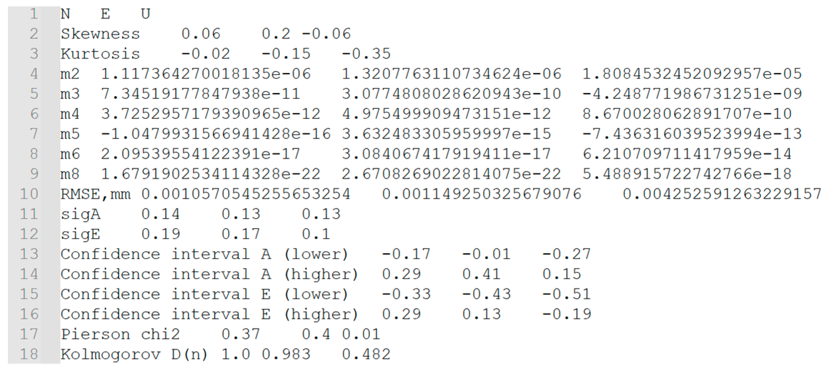
WTZR	N	1.06	0.06 ± 0.14	−0.17, 0.29	−0.02 ± 0.19	−0.33, 0.29
	E	1.15	0.2 ± 0.13	−0.01, 0.41	−0.15 ± 0.17	−0.43, 0.13
	U	4.25	−0.05 ± 0.13	−0.26, 0.16	−0.35 ± 0.1	−0.51, −0.19
HELG	N	1.18	−0.46 ± 0.15	−0.71, −0.21	0.61 ± 0.41	−0.06, 1.28
	E	1.3	0.19 ± 0.15	−0.06, 0.44	0.09 ± 0.26	−0.34, 0.52
	U	4.23	0.11 ± 0.13	−0.1, 0.32	−0.36 ± 0.11	−0.54, −0.18
PTBB	N	1.46	−0.03 ± 0.13	−0.24, 0.18	−0.49 ± 0.1	−0.65, −0.33
	E	1.2	0.07 ± 0.13	−0.14, 0.28	−0.34 ± 0.13	−0.55, −0.13
	U	4.38	−0.11 ± 0.13	−0.32, 0.1	−0.36 ± 0.1	−0.52, −0.2
WROC	N	1.24	−0.17 ± 0.14	−0.4, 0.06	0.16 ± 0.18	−0.14, 0.46
	E	1.19	−0.04 ± 0.14	−0.27, 0.19	0.01 ± 0.2	−0.32, 0.34
	U	4.89	−0.02 ± 0.12	−0.22, 0.18	−0.56 ± 0.08	−0.69, −0.43

.

As can be seen from Table 3, the confidence intervals of the asymmetry for all coordinate components (N, E, U) at each station cover zero, except for HELG. The results of the statistical evaluation can be seen more clearly in

Table 5. PS-NETM conclusion about chosen stations.

Station	EPN Class	Coordinate Components	Overall Conclusion
WTZR	C0	N	There is an effect of weak systematic errors that were not excluded when processing GNSS observations. Evaluation by NETM methods is required.
		E
		U
HELG	C1	N	Significant data pathology. Evaluation is not possible.
		E
		U
PTBB	C5	N	There is an effect of weak systematic errors that were not excluded when processing GNSS observations. Evaluation by NETM methods is required.
		E
		U
WROC	C6	N	There is an effect of weak systematic errors that were not excluded when processing GNSS observations. Evaluation by NETM methods is required.
		E
		U

Here, each of the coordinate components is color-coded according to the diagnostic criteria (see Table 1). When the coordinate component is colored green, it means that confidence intervals for both skewness and kurtosis cover zero, which is the best-case scenario as it indicates that the distribution of residuals of that component is Gaussian. The orange-colored coordinate components are subject to weak systematic errors according to a non-classical approach. Red color marks the worst-case scenario–strong data pathology.

.

It should be noted that the overall conclusion is based on the “worst case” scenario for any of the coordinate components.

4. Discussion

Table 4 clearly shows that there is some data pathology at the HELG station, although it belongs to the highest class C1 in the EPN hierarchy. As for the rest of the stations, the analysis results show that for all three coordinate components, the classical normal error law is inadequate for the real distribution of observational errors. While for the 2D components N and E, the mathematical model of the time series is basically sound, since the confidence intervals of the skewness and kurtosis cover zero, the altitude component U is obviously affected by unaccounted-for systematic errors. The performance of the PTBB station corresponds to its class: each component is affected by unaccounted-for systematic errors, as can be seen from the analysis of confidence intervals and the PS-NETM conclusion.

The time series graphs, along with histograms for each station, are present in Appendix A.

5. Conclusions

The statistical analysis of the GNSS time series holds paramount importance in the field of Space Geodesy, serving as a cornerstone for extracting meaningful information from the vast and intricate datasets generated by Global Navigation Satellite Systems. The utilization of statistical methods in the analysis of GNSS time series is multifaceted, addressing various challenges inherent in the measurements and providing valuable insights into the Earth’s dynamic processes.

This paper presents the main ideas of the non-classical measurement theory and a software solution for their practical implementation in the field of the metrological diagnostics of long-time series obtained at permanent GNSS stations for different levels. To analyze the presence of residual unaccounted-for systematic errors at a particular GNSS station, we propose a new software package called PS-NETM (Python software—Non-classical Error Theory of Measurements). Its main functionalities are summarized, and a numerical example is given to demonstrate the software’s capabilities in terms of diagnosing the probabilistic form of measurement distributions, which is based on the use of confidence intervals for estimating the skewness and kurtosis of large samples, followed by the application of Pearson’s χ2 test.

Based on this example, it can be argued that the distribution of errors for the selected time series of permanent GNSS stations in Europe is not perfect and does not follow the law of normal distribution.

The results of this work reveal a large problem with the current GNSS time series, which is unaccounted-for small systematic errors. We feel it is vital to make such an analysis before conducting any experiments on a particular GNSS station. The research shows that the C1 station HELG, which is considered very reliable by EPN, has some data pathology. In other words, some large systematic errors are present there. These might include multipath effects, unreliable antenna placement, the movement of underground waters, which disturb the antenna, etc. The sources of such errors should be investigated individually at each station.

References

- Bock, Y.; Wdowinski, S. GNSS Geodesy in Geophysics, Natural Hazards, Climate, and the Environment. In Position, Navigation, and Timing Technologies in the 21st Century: Integrated Satellite Navigation, Sensor Systems, and Civil Applications; IEEE: Piscataway, NJ, USA, 2020; pp. 741–820. [Google Scholar] [CrossRef]
- He, X.; Montillet, J.-P.; Fernandes, R.; Bos, M.; Yu, K.; Hua, X.; Jiang, W. Review of current GPS methodologies for producing accurate time series and their error sources. J. Geodyn. 2017, 106, 12–29. [Google Scholar] [CrossRef]
- Dong, D.; Fang, P.; Bock, Y.; Webb, F.; Prawirodirdjo, L.; Kedar, S.; Jamason, P. Spatiotemporal filtering using principal component analysis and Karhunen-Loeve expansion approaches for regional GPS network analysis. J. Geophys. Res. Solid Earth 2006, 111, B03405. [Google Scholar] [CrossRef]
- Ming, F.; Yang, Y.; Zeng, A.; Zhao, B. Spatiotemporal filtering for regional GPS network in China using independent component analysis. J. Geod. 2017, 91, 419–440. [Google Scholar] [CrossRef]
- Zhou, M.; Guo, J.; Shen, Y.; Kong, Q.; Yuan, J. Extraction of common mode errors of GNSS coordinate time series based on multi-channel singular spectrum analysis. Chin. J. Geophys. 2018, 61, 4383–4395. [Google Scholar] [CrossRef]
- Tian, Y.; Shen, Z.-K. Extracting the regional common-mode component of GPS station position time series from dense continuous network. J. Geophys. Res. Solid Earth 2016, 121, 1080–1096. [Google Scholar] [CrossRef]
- Bos, M.S.; Montillet, J.P.; Williams, S.D.P.; Fernandes, R.M.S. Introduction to Geodetic Time Series Analysis; Springer: Cham, Switzerland, 2019; pp. 29–52. [Google Scholar] [CrossRef]
- King, M.A.; Watson, C.S. Long GPS coordinate time series: Multipath and geometry effects. J. Geophys. Res. Solid Earth 2010, 115, 2500–2511. [Google Scholar] [CrossRef]
- Wu, D.; Yan, H.; Shen, Y. TSAnalyzer, a GNSS time series analysis software. GPS Solut. 2017, 21, 1389–1394. [Google Scholar] [CrossRef]
- Santamaría-Gómez, A. SARI: Interactive GNSS position time series analysis software. GPS Solut. 2019, 23, 52. [Google Scholar] [CrossRef]
- He, X.; Yu, K.; Montillet, J.-P.; Xiong, C.; Lu, T.; Zhou, S.; Ma, X.; Cui, H.; Ming, F. GNSS-TS-NRS: An Open-Source MATLAB-Based GNSS Time Series Noise Reduction Software. Remote Sens. 2020, 12, 3532. [Google Scholar] [CrossRef]
- Łyszkowicz, A.; Pelc-Mieczkowska, R.; Bernatowicz, A.; Savchuk, S. First results of time series analysis of the permanent GNSS observations at polish EPN stations using GipsyX software. Artif. Satell. 2021, 56, 101–118. [Google Scholar] [CrossRef]
- Zus, F.; Dick, G.; Dousa, J.; Wickert, J. Systematic errors of mapping functions which are based on the VMF1 concept. GPS Solut. 2015, 19, 277–286. [Google Scholar] [CrossRef]
- Langbein, J.; Svarc, J.L. Evaluation of temporally correlated noise in global navigation satellite system time series: Geodetic monument performance. J. Geophys. Res. Solid Earth 2019, 124, 925–942. [Google Scholar] [CrossRef]
- Geng, J.; Chen, X.; Pan, Y.; Mao, S.; Li, C.; Zhou, J.; Zhang, K. PRIDE PPP-AR: An open-source software for GPS PPP ambiguity resolution. GPS Solut. 2019, 23, 91. [Google Scholar] [CrossRef]
- Bock, Y.; Fang, P.; Knox, A.; Sullivan, A.; Jiang, S.; Guns, K.; Golriz, D.; Moore, A.; Argus, D.; Liu, Z.; et al. Extended Solid Earth Science ESDR System: Algorithm Theoretical Basis Document. 2023. Available online: http://garner.ucsd.edu/pub/measuresESESES_products/ATBD/ESESES-ATBD.pdf (accessed on 12 June 2023).
- Barba, P.; Rosado, B.; Ramírez-Zelaya, J.; Berrocoso, M. Comparative Analysis of Statistical and Analytical Techniques for the Study of GNSS Geodetic Time Series. Eng. Proc. 2021, 5, 21. [Google Scholar] [CrossRef]
- Time Series in SOPAC Archive. Available online: http://garner.ucsd.edu/pub/measuresESESES_products/Timeseries/ (accessed on 12 June 2023).
- Jeffreys, H. The law of error and the combination of observations. Philos. Trans. R. Soc. Lond. Ser. A Math. Phys. Sci. 1938, 237, 231–271. [Google Scholar] [CrossRef]
- Dvulit, P.; Dzhun, J. Application of methods of the non-classical error theory in absolute measurements of Galilean acceleration. Geodynamics 2017, 1, 7–15. [Google Scholar] [CrossRef]
- Chimitova, E.; Lemeshko, B.; Lemeshko, S.; Postovalov, S.; Rogozhnikov, A. Software System for Simulation and Research of Probabilistic Regularities and Statistical Data Analysis in Reliability and Quality Control. In Mathematical and Statistical Models and Methods in Reliability: Applications to Medicine, Finance, and Quality Control; Birkhäuser: Boston, MA, USA, 2014; Volume 114, pp. 417–432. [Google Scholar] [CrossRef]
- Tumanov, A.; Sabanaev, A.; Solovyov, A.; Tumanov, V. Statistical testing of hypotheses about the form of the factor law of influence by the Kolmogorov criterion. J. Phys. Conf. Ser. 2020, 1614, 012082. [Google Scholar] [CrossRef]
- Lee, G.; Gommers, R.; Wasilewski, F.; Wohlfahrt, K.; O’Leary, A. PyWavelets: A Python package for wavelet analysis. J. Open Source Softw. 2019, 4, 1237. [Google Scholar] [CrossRef]
- Huang, N.E.; Shen, Z.; Long, S.R.; Wu, M.C.; Shih, H.H.; Zheng, Q.; Yen, N.C.; Tung, C.C.; Liu, H.H. The empirical mode decomposition and the Hilbert spectrum for nonlinear and non-stationary time series analysis. Proc. R. Soc. Lond. Ser. A Math. Phys. Eng. Sci. 1998, 454, 903–995. [Google Scholar] [CrossRef]
- Ji, K.; Shen, Y. A Wavelet-Based Outlier Detection and Noise Component Analysis for GNSS Position Time Series. In Beyond 100: The Next Century in Geodesy. International Association of Geodesy Symposia; Freymueller, J.T., Sánchez, L., Eds.; Springer: Cham, Switzerland, 2020; Volume 152. [Google Scholar] [CrossRef]
- Time Series in CDDIS Archive. Available online: https://cddis.nasa.gov/archive/GPS_Explorer/archive/time_series/ (accessed on 12 June 2023).
- Reference Stations Classification in EPN. Available online: http://www.epncb.oma.be/_productsservices/ReferenceFrame/Station_Classification.php (accessed on 12 June 2023).