Article

SSAformer: Spatial–Spectral Aggregation Transformer for Hyperspectral Image Super-Resolution

1
College of Advanced Interdisciplinary Studies, National University of Defense Technology, Changsha 410073, China
2
State Key Laboratory of Pulsed Power Laser Technology, Changsha 410073, China
3
Hunan Provincial Key Laboratory of High Energy Laser Technology, Changsha 410073, China
4
The State Key Laboratory of High Performance Computing, College of Computer Science and Technology, National University of Defense Technology, Changsha 410073, China
*
Author to whom correspondence should be addressed.
These authors contributed equally to this work.
Remote Sens. 2024, 16(10), 1766; https://doi.org/10.3390/rs16101766
Submission received: 28 March 2024 / Revised: 13 May 2024 / Accepted: 14 May 2024 / Published: 16 May 2024
(This article belongs to the Special Issue Deep Learning for the Analysis of Multi-/Hyperspectral Images II)

Abstract

:
The hyperspectral image (HSI) distinguishes itself in material identification through its exceptional spectral resolution. However, its spatial resolution is constrained by hardware limitations, prompting the evolution of HSI super-resolution (SR) techniques. Single HSI SR endeavors to reconstruct high-spatial-resolution HSI from low-spatial-resolution inputs, and recent progress in deep learning-based algorithms has significantly advanced the quality of reconstructed images. However, convolutional methods struggle to extract comprehensive spatial and spectral features. Transformer-based models have yet to harness long-range dependencies across both dimensions fully, thus inadequately integrating spatial and spectral data. To solve the above problem, in this paper, we propose a new HSI SR method, SSAformer, which merges the strengths of CNNs and Transformers. It introduces specially designed attention mechanisms for HSI, including spatial and spectral attention modules, and overcomes the previous challenges in extracting and amalgamating spatial and spectral information. Evaluations on benchmark datasets show that SSAformer surpasses contemporary methods in enhancing spatial details and preserving spectral accuracy, underscoring its potential to expand HSI’s utility in various domains, such as environmental monitoring and remote sensing.

1. Introduction

A hyperspectral image(HSI) creates a three-dimensional data cube, where each pixel is represented by an almost continuous spectral curve. This representation captures the spatial arrangements and spectral characteristics so that the objects can be differentiated clearly. High-resolution (HR) remote sensing images, crucial in applications like military rescue [1] and environmental monitoring [2], provide detailed observations of ground objects. These images facilitate various tasks, including image classification [3], object detection [4], and tracking [5]. However, the limitations posed by sensors and transmission bandwidth necessitate a trade-off between spatial and spectral resolutions. The spatial resolution is often reduced to preserve accurate spectral features, causing a significant challenge in enhancing HSI spatial resolution. In recent years, multiple strategies have been proposed to address the issue of low spatial resolution in HSIs, broadly divided into two categories. The first approach employs fusion methods [6], which integrate image data from diverse sources to extract and amalgamate valuable information within a unified framework, thus producing HR HSIs enriched with spatial details and spectral data. The second strategy involves single HSI super-resolution (SR), aimed at directly producing HSIs with enhanced spatial resolution by learning the mapping relations between low-resolution (LR) HSIs and their HR counterparts. For fusion-based methods, the traditional approach typically relies on preset algorithms to integrate images of different resolutions. These techniques are effective in specific cases but usually require precise image alignment and complex preprocessing steps, which may be difficult to meet in dynamic or complex environments, limiting their application scope. In contrast, fusion methods based on deep learning automatically extract and integrate features by learning from a large amount of data. This approach not only improves the accuracy of fusion but also handles larger datasets better, better adapting to changing environmental conditions. Nevertheless, fusion-based methods can offer richer information but face major challenges: accurate alignment of different source images is critical but hard in dynamic environments, risking data loss. Additionally, the heterogeneity of sources complicates fusion, requiring extensive preprocessing [7]. Conversely, single HSI SR is more straightforward, eliminating the need for auxiliary data or complex preprocessing and dominating in current research with its simplicity implemented by deep learning techniques.
Traditional single HSI SR methods develop a mapping function from LR to HR HSIs, often relying on handcrafted prior knowledge (e.g., low-rank approximations [8] and sparse coding [9]) to address the inherent uncertainty in HR-HSI reconstruction. In these methods, prior knowledge acts as regularization to simulate image degradation in a forward mathematical model that captures the spectral properties and spatial structure of the input. However, the optimization of the model is often ill-conditioned, and it is difficult to solve the optimal HR-HSI results. Moreover, although various priors [10,11], such as spectral mixing models, total variation, sparse representation, low rank, and self-similarity, have been explored in signal processing and computer vision, demonstrating superiority over unconstrained optimization techniques, the diversity of HSI scenarios and the intricate nature of spectral and spatial structures pose challenges in the efficient designs of priors.
Benefiting from the end-to-end learning of a mapping function implemented by deep learning techniques, the spatial–spectral features of HSIs could be captured adeptly without handcrafted priors. With developments in computing hardware and the increase in available datasets, deep learning has set new benchmarks in HSI SR. Among the leading architectures in this domain are convolutional neural networks (CNNs) and Transformers.
The CNN, known for its deep structures and convolutional operations, excels at extracting depth-wise features from images and understanding the mapping relations between LR-HSI and HR-HSI, effectively representing spatial–spectral relationships. The emergence of SRCNN [12] has inspired many CNN-based methods, incorporating advanced techniques like residual learning [13], attention mechanisms [14,15], and multiscale processing [16,17,18] to boost performance. Some researchers have also explored 3D convolutions to address spectral-wise representations [19,20] and minimize spectral distortions. Nonetheless, CNNs, primarily focusing on local feature extraction, may perform suboptimally in extracting long-range information in HSIs, resulting in poor representational capacity and artifacts in HSI SR outcomes.
Recently, Transformers have been applied to single HSI SR, leveraging self-attention mechanism that grasp long-range dependencies and integrate information globally, enhancing the quality of HR HSI reconstruction. Despite their scalability and flexibility, the applicability of Transformers in HSI-SR is hampered by the limited size of HSI datasets compared to the vast collections of RGB images. Moreover, the computational complexity of Transformers, which scales quadratically with the sequence length O ( N 2 ) , imposes significant computational demands.
To address the aforementioned challenges, including the inadequacy of CNNs in capturing long-range dependencies, the high computational cost of Transformers in processing large-scale HSI data, and the existing room for improvement in the extraction and fusion of spatial and spectral information in HSI SR tasks, we introduce Spatial–Spectral Aggregation Transformer (SSAformer), a hybrid model that combines the strengths of Transformer and CNN architectures for efficient feature extraction and fusion in spatial–spectral channels, achieving superior restoration results. Specifically, SSAformer incorporates spatial and spectral attention modules. For spatial features, it introduces a window attention mechanism for enhanced extraction and employs a cross-fusion attention mechanism to strengthen long-range dependencies. This approach not only maintains linear computational complexity but also broadens the receptive field, effectively reducing spatial artifacts. In the spectral domain, SSAformer applies channel attention operations via deformable convolutions (DCs), adaptively processing information from each channel to overcome the redundancy inherence in HSIs. Consequently, SSAformer tackles channel redundancy and significantly improves global attention to spectral features. Comprehensive experiments on three widely used benchmark datasets show that SSAformer surpasses existing state-of-the-art (SOTA) methods. Our contributions can be summarized as follows:
  • We propose the novel Spatial–Spectral Aggregation Transformer for HSI SR, designed to capture and integrate long-range dependencies across spatial and spectral dimensions. It features spatial and spectral attention modules that effectively extract and integrate spatial and spectral information in HSI SR tasks, significantly enhancing SR performance while maintaining linear computational complexity.
  • To achieve long-range spatial dependencies, we construct spatial attention modules, utilizing cross-range spatial self-attention mechanisms within cross-fusion windows to aggregate local and global features, effectively enhancing the model’s perception of spatial details while ensuring the integrity and continuity of spatial information.
  • To address the redundancy problem in high-dimensional spectral data of HSIs and effectively capture long-range spectral dependencies, we construct spectral attention modules, combining DCs to perform spatial attention operations, reducing channel redundancy while enhancing the model’s global attention to spectral characteristics.

2. Related Work

In this section, we review the significant advancements in the research field of HSI SR. We first outline the two primary directions of HSI SR research: fusion-based approaches and single HSI SR methods. Subsequently, we focus on single HSI SR methods based on deep learning.

2.1. Hyperspectral Image Super-Resolution

The field of HSI SR is mainly divided into two directions [7]: fusion-based methods and single HSI SR methods. Fusion-based methods enhance spatial resolution by fusing an additional high-spatial-resolution image (e.g., an RGB or multispectral image) with an LR HSI. This approach utilizes various techniques including panchromatic sharpening [21], Bayesian inference [22], matrix [23] and tensor decomposition [24], and deep learning [25]. In contrast, single HSI SR methods aim to reconstruct HR images directly from LR HSIs. The challenge lies in recovering rich high-frequency details from limited spatial details while maintaining the integrity of spectral information. Given the limitations of hyperspectral and multispectral fusion tasks in fully exploiting spectral correlations and the resultant spectral distortions, we focus on single HSI SR methods.

2.2. Traditional Methods for Single HSI SR Methods

Traditional methods typically enhance image spatial resolution through mathematical and signal processing techniques, treating HSI SR as an optimization problem. Constraints on the optimization process are imposed by various image priors to obtain the desired representation of the HSIs. These techniques include projection-based methods [26], sparse representation [22], dictionary learning [27], and matrix factorization [28], leveraging well-designed priors like image self-similarity, sparsity, and low-rank properties to guide the reconstruction process. Notable works include the HSI acquisition model [29] and the Projection Onto Convex Sets (POCS) algorithm to reconstruct the HR HSI [26]. Akhtar et al. [22] introduced a sparse representation-based HSI SR method, interpreting high-spatial-resolution images through extracted spectra. Liu et al.,’s trainable grouped joint tensor dictionary precisely maps LR to HR HSIs in limited training samples [27]. Yokoya et al. offered a coupled non-negative matrix factorization hybrid approach for HSI data fusion [30]. He et al. introduced a coupled tensor ring decomposition method for SR improvements [31]. Although traditional single HSI SR methods have shown potential to leverage handmade image priors to solve complex optimization problems, their reliance on specific image priors and degenerate models, as well as limitations in dealing with complex or unknown image structures, have ultimately led to the introduction and rapid development of deep learning methods.

2.3. Deep Learning Methods for Single HSI SR Methods

Unlike leveraging handcrafted image priors, deep learning networks can automatically learn those underlying image priors hidden in training data, successfully applied to HSI SR tasks, and offer superior SR performance. Since CNNs and Transformers are attracting increasing attention, this section introduces those single HSI SR works based on the two models.

2.3.1. CNN-Based Single Hyperspectral Image Super-Resolution

In recent years, deep learning methods have achieved remarkable success in natural image SR, primarily due to the powerful representational ability of CNNs. These CNN-based methods aim to learn the mapping function between LR and HR images through supervised learning. Since Dong et al. [32] introduced the CNN into the image SR task in 2014, CNN-based methods have developed rapidly to study single RGB image SR. Inspired by these methods, various HSI SR approaches have been proposed. For instance, Yuan et al. [33] and Xie et al. [28] first performed SR on HSI based on DCNNs, followed by applying non-negative matrix factorization to ensure the spectral characteristics of the intermediate results. Li et al. [34] introduced a new grouped deep recursive residual network to enhance SR performance. Jiang et al. [14] proposed a progressive multibranch network to learn the spatial–spectral priors of grouped spectra (SSPSR). Jia et al. [35] proposed a spectral–spatial network for HSI SR, effectively improving spatial resolution while retaining spectral information. In addressing the HSI-SR problem, although traditional CNN methods can effectively extract HSI spatial features, 2D convolution is less effective in preserving reconstructed HSI spectral information. Given the numerous channels in the spectral dimension of HSIs, applying 3D convolutional networks to simultaneously capture spatial and spectral features and utilizing residual learning strategies to deepen model layers can significantly improve the overall quality of SR images. For example, Mei et al. [19] proposed the 3D Fully Convolutional Network (3DFCNN), which directly extracts spatial–spectral features through 3D convolution to leverage high-dimensional spectral properties. Li et al. [20] designed the Mixed Convolution Network (MCNet), which extracts spatial and spectral information through a mix of 2D and separable 3D convolutions. Li et al. [34] further developed the Grouped Deep Recursive Residual Network (GDRRN), which replaces 3D convolution by introducing grouped convolutions into recursive residual modules. However, these mainstream techniques have not yet overcome the inherent limitations of CNNs. They perform poorly in capturing long-range dependencies and establishing associations between space and spectra, which limits the full utilization of spectral information and may lead to undesirable artifacts in the SR image reconstruction process.

2.3.2. Transformer-Based Single Hyperspectral Image Super-Resolution

Initially proposed in the field of natural language processing [36,37,38,39], the Transformer’s exceptional ability to handle nonlocal similarities was discovered and was applied in HSI SR tasks after achieving tremendous success in computer vision tasks.
Some researchers have combined Transformers with 3D convolution to learn spatial–spectral features. For example, Liu et al. [40] designed a parallel branch network called Interactformer, which combines transformer modules with 3D convolution. Hu et al. [41] proposed a multilevel progressive network (MPNet), employing progressive learning and nonlocal channel attention to learn details. Wang et al. [42] also combined spectral-oriented self-attention with 3D convolution, called 3DTHSR, to learn spatial–spectral features within a global receptive field. However, due to the quadratic computational complexity of attention, these methods have high computational complexity and only explore long-range dependencies in the spectral dimension, thus failing to fully utilize global and local spatial information. Some researchers have made improvements, such as Geng et al. [43], who used matrix factorization to replace the original self-attention, modeling dependencies between different tokens. Similarly, self-attention was approximated as a linear dot product of kernel feature maps to avoid the massive computation in attention [44]. ESSA [45] took hyperspectral characteristics into account, bringing channel-wise inductive biases to the model. However, these network models often focus more on extracting spectral information and fail to pay sufficient attention to spatial information both locally and globally. Therefore, to fully extract and fuse spatial and spectral information, we introduce a spatial–spectral aggregate Transformer model, SSAformer, to leverage local–global spatial–spectral information.

3. Methodology

In this section, we describe the details of the proposed SSAformer: Spatial–Spectral Aggregation Transformer. This framework is conceived to address the challenge of effectively capturing and integrating both spatial and spectral information within an HSI through the strategic integration of attention-based mechanisms.

3.1. Overall Architecture

As shown in Figure 1, the overall network architecture of SSAformer comprises three modules: shallow feature extraction (the initial convolution layer immediately following the input), deep feature extraction (the middle part of the figure, highlighted with a shaded area in Figure 1a), and image reconstruction (the final set of layers consisting of a convolution layer, PixelShuffle, followed by another convolution layer). The procedure begins with an LR hyperspectral input image, I L R R H × W × B , where H, W, and B signify the image’s height, width, and number of spectral bands, respectively. A convolutional operation initially processes the input to extract shallow features F i n i t , described by
F i n i t = H c o n v ( I L R ) ,
where H c o n v denotes the convolutional layer for initial feature extraction.
Subsequently, these initial features undergo refinement through the deep feature extraction module, which aims to enhance spatial and spectral details, yielding the deep features F d f :
F d f = H D F E ( F i n i t ) ,
with H D F E ( · ) representing the operations within the deep feature extraction module. As depicted in Figure 1b, the spatial–spectral attention group (SSAG) module comprises several spatial–spectral attention blocks (SSABs), interspersed with convolutional layers and element-wise summations, to progressively refine the feature representation. As illustrated in Figure 1c, each SSAB contains spatial and spectral attention modules, which are the core of the algorithm, and also includes conventional residual connections, multilayer perceptrons (MLPs), and layer normalization.
The last process is the reconstruction of an HR HSI I H R R H × W × B , where H and W are the enhanced spatial dimensions:
I H R = H u p s a m p l e ( F d f ) ,
Here, H u p s a m p l e embodies the upsampling operations, including PixelShuffle and convolutional layers, as depicted on the right of Figure 1a.
Overall, SSAformer integrates the current mainstream architectures for image restoration, effectively extracting and aggregating spatial and spectral information in the deep feature extraction module, which is detailed in Section 3.2 and Section 3.3.

3.2. Spectral Attention Block

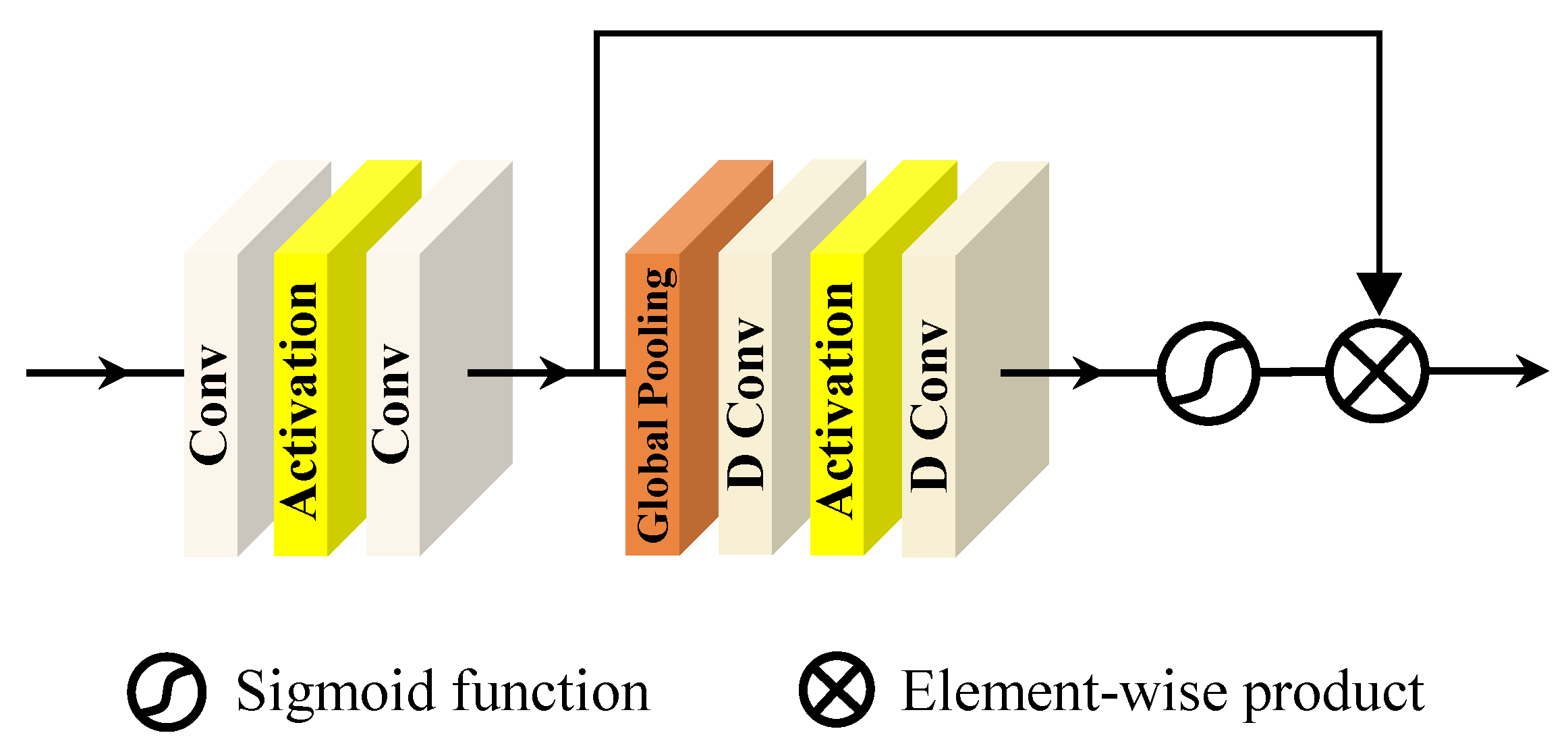
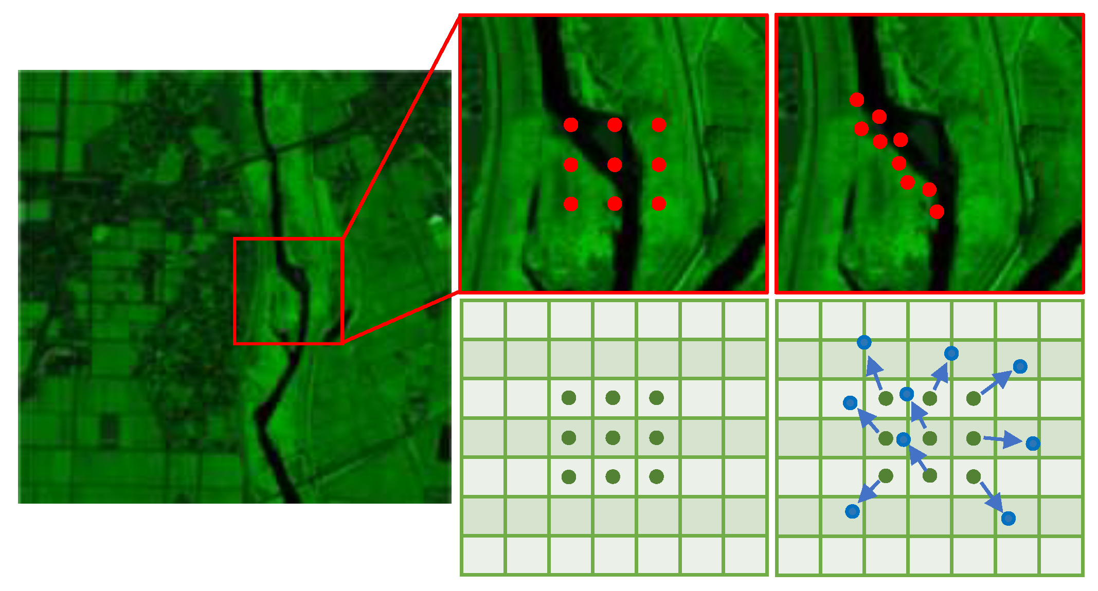
The Spectral attention block (SEB) is specifically designed as an adaptive channel-wise feature extraction mechanism within the network, and its structure is shown in Figure 2. This module starts with two convolution layers and an activation function to generate preliminary spectral feature maps. Global pooling then aggregates global contextual information. Subsequent DC [46] layers are set to adaptively learn the key information of each channel, selectively emphasizing relevant spectral features while suppressing irrelevant ones, thus enhancing channel feature selection. As illustrated in Figure 3, DC can dynamically modify the positions of their sampling points during convolutional operations. The direction and distance of the movements of these sampling points are learnable parameters. With continuous learning by the network, DC can more comprehensively extract detail information such as edges, textures, and other features. After extracting features from all channels, the module extensively learns the most informative spectral features. Finally, the sigmoid activation function ensures that only the most essential features are passed on, implementing spectral attention effectively within the network. The use of DC endows SEB to focus on detailed features in different spectral channels, thereby achieving the goal of spectral attention and enhancing the richness of HSI representation.

3.3. Spatial Attention Block

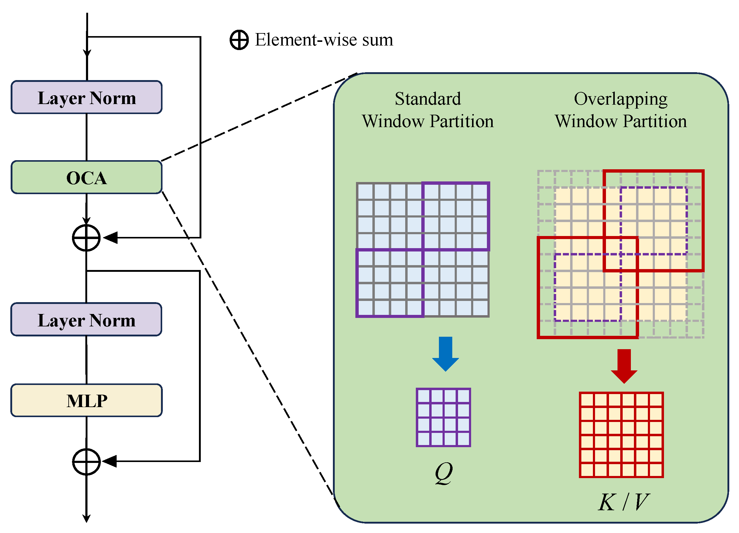
The spatial attention block (SAB) is strategically integrated into our network architecture to enhance spatial feature extraction capabilities, drawing upon the principles of the Swin Transformer [47], as shown in Figure 4. Central to the SAB is the overlapping cross-attention (OCA), which is designed to establish essential cross-window connections that bolster the representational efficacy of window self-attention mechanisms. The SAB combines an OCA layer with a multilayer perceptron, along with necessary layer normalization and residual connections.
The disparate window size to segment the projected features is the core of the OCA’s innovative approach. For an input feature X, with constituent elements X Q , X K , X V R H × W × C , X Q is partitioned into H W M 2 nonoverlapping windows of size M × M , while X K and X V are expanded into H W M 2 overlapping windows of size M o × M o . The overlap is mathematically expressed as
M o = ( 1 + γ ) × M ,
where M denotes the original window size, and γ is a constant governing the extent of the overlap.
This overlapping window partitioning scheme is conceptualized as a sliding window operation with a kernel size equivalent to M o and a stride equal to M, supplemented by zero-padding of size γ M 2 to ensure the size consistency of overlapping windows. The attention matrix is computed as outlined in Equation (5):
Attention ( Q , K , V ) = SoftMax Q K T d + B V .
The relative position bias B R M × M o is also incorporated. Unlike traditional window self-attention, where queries, keys, and values originate from identical window features, the OCA formulates keys/values from an expanded field, thereby providing query access to a more extensive and informative context. It is important to note that the work on OCA is derived from [48].
With its OCA core, the SAB essentially signifies an advanced iteration of spatial attention methodologies. By converging the spatial discernment of the SAB with the spectral acuity of the SEB, our framework is adeptly engineered to exhaustively characterize the features of HSIs.

3.4. Loss Function

Pioneering studies have underscored the efficacy of L 1 and L 2 losses in SR tasks [15,49]. Given the propensity of the L 2 norm to yield oversmoothing, our approach is based on the L 1 norm owing to its promotion of a more equitable error spread and enhanced iterative convergence. The accuracy of SR image reconstruction is gauged using the L 1 norm, which calculates the pixelwise difference between the reconstructed SR hyperspectral images and original HR hyperspectral images, depicted as
L pix ( Φ ) = 1 N i = 1 N R h r i R s r i 1 ,
where N denotes the total number of images within a batch, Φ represents our network’s parameter ensemble, R h r i is the i th HR image, and R s r i is its SR counterpart. Although L pix is adept for SR in standard imaging, its neglect of HSI spectrality may precipitate spectral fidelity degradation [15]. To circumvent this, we introduce a spectral coherence loss, termed SAM loss, to safeguard the spectral integrity and detail precision, formulated as
L spec ( Φ ) = 1 N i = 1 N 1 π arccos R h r i · R s r i R h r i 2 R s r i 2 .
To refine the image’s textural acuity, we borrow insights from the work of Wang et al. [50], integrating gradient details by evaluating differences between adjacent pixel values. The gradient map of an HSI R is formulated as
Δ R = ( Δ x R , Δ y R , Δ z R ) ,
N ( R ) = Δ R 2 ,
In this context, N ( · ) functions to extract the gradient field of R, while Δ x , Δ y , and Δ z are the operators computing the gradient magnitudes along the horizontal, vertical, and spectral planes, respectively. Employing a gradient-based loss, L grad , we aim to reduce the deviation between the gradient fields of SR and original HR images, thus enhancing edge definition in the enlarged images:
L grad ( Φ ) = 1 P i = 1 P N ( R h r i ) N ( R s r i ) 1 .
Conclusively, the network’s training is governed by a comprehensive loss function, L overall , which amalgamates the losses above, duly weighted:
L overall ( Φ ) = L pix + ω 1 L spec + ω 2 L grad ,
where ω 1 and ω 2 serve as the balancing coefficients for the spectral and textural components, respectively. These coefficients are provisionally set to ω 1 = 0.5 and ω 2 = 0.1 , demonstrating optimal SR results in rendering both spatial and spectral detail intricacies.

4. Experiments and Analysis

In this section, we conduct comprehensive experiments to evaluate the effectiveness of the proposed SSAformer. We use three benchmark datasets, Chikusei [51], Houston2018 [52], and Pavia Centre [53], for comparisons. We present the quantitative and visual results of our SSAformer alongside five existing HSI SR methods, including bicubic interpolation, 3DFCNN [19], GDRRN [34], SSPSR [14], and MSDformer [15].

4.1. Datasets

(a)
Chikusei dataset [51]: The Chikusei dataset captures a wide array of urban and agricultural landscapes in the Chikusei area, Ibaraki Prefecture, Japan. The dataset spans a wavelength range from 363 nm to 1018 nm with 128 spectral bands. Each image boasts a high spatial resolution of 2048 × 2048 pixels. The images encompass diverse scenes, including urban areas, rice fields, forests, and roads, making it suitable for various remote sensing applications.
(b)
Houston2018 dataset [52]: The Houston2018 dataset presents hyperspectral urban images collected over the University of Houston campus and the neighboring urban area. This dataset was captured by the ITRES CASI-1500 (ITRES Research Limited, Calgary, Alberta, Canada) hyperspectral sensor, covering a spectral range from 380 nm to 1050 nm across 48 bands. The spatial resolution of the images is 4172 × 1202 pixels. Each image in this collection has a spatial resolution of 1 m per pixel.
(c)
Pavia Centre dataset [53]: The Pavia Centre dataset was acquired over the urban center of Pavia, northern Italy, through the Reflective Optics System Imaging Spectrometer (ROSIS). The HSIs in this dataset cover a wavelength range of 430 nm to 860 nm, divided into 102 bands after removing noisy bands. The spatial resolution of the dataset is 1.3 m per pixel, with image dimensions of 1096 × 1096 pixels.

4.2. Implementation Details

In our proposed network, the number of channels in the SSAG is set to 180, and the number of consecutive SSAGs and SSABs is set to 4. The attention heads are also set to 4. In OCA, the overlapping scale parameter is set to 0.5. In the loss function formulation, we set the weights ω 1 = 0.5 and ω 2 = 0.1 . We adopt the Adam optimizer with β 1 = 0.9 and β 2 = 0.99 to train the model for 300 epochs. The initial learning rate is set to 5 × 10 5 , which decays by a factor of ten after 150 epochs. The proposed model is implemented in PyTorch=1.9.0 on an NVIDIA RTX 4090 GPU.

4.3. Evaluation Metrics

We utilize six established metrics to comprehensively evaluate the quality of HSIs, considering both spatial and spectral dimensions. These metrics include the peak signal-to-noise ratio (PSNR), which measures the maximum possible pixel value against the mean squared error; the structure similarity (SSIM) index [54], which compares the similarity of image structures; the spectral angle mapper (SAM) [55], assessing spectral similarity; the cross correlation (CC) [56], quantifying the correlation between the SR results and HR images; the root mean squared error (RMSE), indicating the standard deviation of the residuals; and the erreur relative globale adimensionnelle de synthèse (ERGAS) [57], a dimensionless global relative error of synthesis that provides an overall quality measure. The mathematical formulations of these metrics are defined as follows:
P S N R = 1 L l = 1 L 10 log 10 M A X l 2 M S E l ,
M S E l = 1 W H w = 1 W h = 1 H I S R ( w , h , l ) I H R ( w , h , l ) 2 ,
R M S E l = M S E l ,
S S I M = 1 L l = 1 L ( 2 μ I S R l μ I H R l + c 1 ) ( 2 σ I S R l I H R l + c 2 ) ( μ I S R l 2 + μ I H R l 2 + c 1 ) ( σ I S R l 2 + σ I H R l 2 + c 2 ) ,
S A M = arccos I S R l , I H R l I S R l 2 I H R l 2 ,
C C = 1 L l = 1 L cov ( I S R l , I H R l ) σ I S R l σ I H R l ,
E R G A S = 100 s 1 L l = 1 L R M S E l mean ( I H R l ) 2 ,
where L represents the total number of spectral bands, W and H denote the image width and height, M A X l is the maximum pixel value within the l-th band, μ and σ correspond to the mean and standard deviation, respectively, and s is the scale factor reflecting the sensor’s spatial resolution. Constants c 1 and c 2 are included to stabilize the division with small denominators in the SSIM formula. These metrics together provide a robust framework for quantifying the performance of image reconstruction algorithms.

4.4. Comparison with State-of-the-Art SR Methods

4.4.1. Experiments on the Chikusei Datasets

For ease of performance comparison, we adopted the data preprocessing method from [14,15,50]. Specifically, due to the irrelevance of information in edge areas, we cropped the center region of the original scenes, resulting in an area of 2304 × 2048 × 128. The top section of the cropped images was further segmented into four nonoverlapping HSIs of 512 × 512 × 128 each. Corresponding LR HSIs were generated by bicubic downsampling at various scale factors.
The remainder of each image was cropped into overlapping patches for training purposes, with 10% randomly selected as a validation set. Specifically, for a scale factor of ×2, patches of 64 × 64 × 128 with an overlap of 32 pixels were used. For a scale factor of ×4, patches of 128 × 128 × 128 with an overlap of 64 pixels were used. For a scale factor of ×8, patches of 256 × 256 × 128 with an overlap of 128 pixels were utilized. These patches served as the ground truth, with corresponding LR HSIs also generated by bicubic downsampling at respective scale factors.
Table 1 displays quantitative results on the Chikusei dataset [51] for our method and other comparative methods at different scale factors, with the best results bolded and the second-best underlined. Notably, bicubic (nondeep learning method) showed average SR performance, while deep learning approaches achieved significant improvements. SSPSR [14] utilized a grouping strategy to extract spectral information, achieving good SR results effectively. MSDformer [15], building on the grouping strategy with the addition of a Transformer, captured long-range dependencies of spectral information but lacked attention to local spatial details. Significantly, the proposed SSAformer, by capturing global spatial–spectral dependencies, demonstrated superior spatial–spectral information extraction and fusion capabilities, outperforming other methods across all metrics, whether at scale factors of ×2, ×4, or ×8.
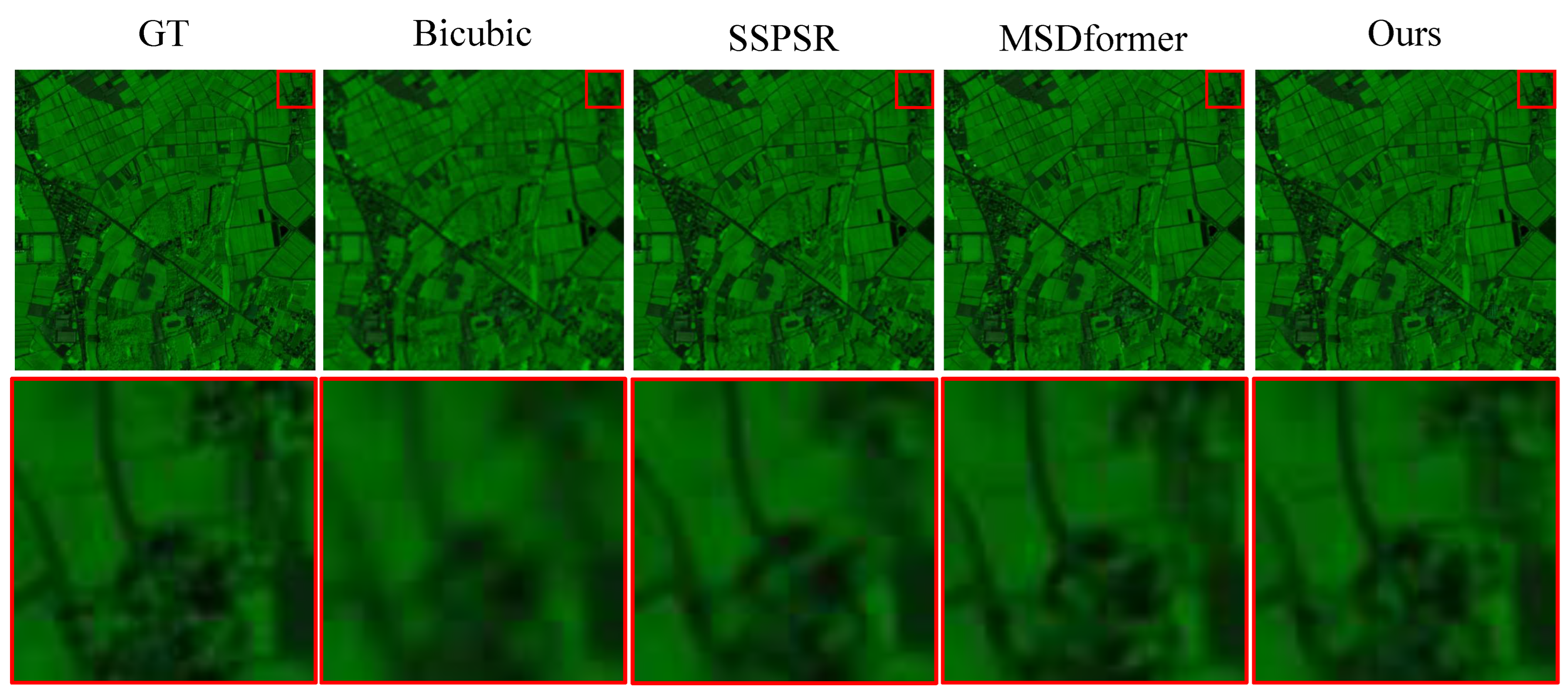
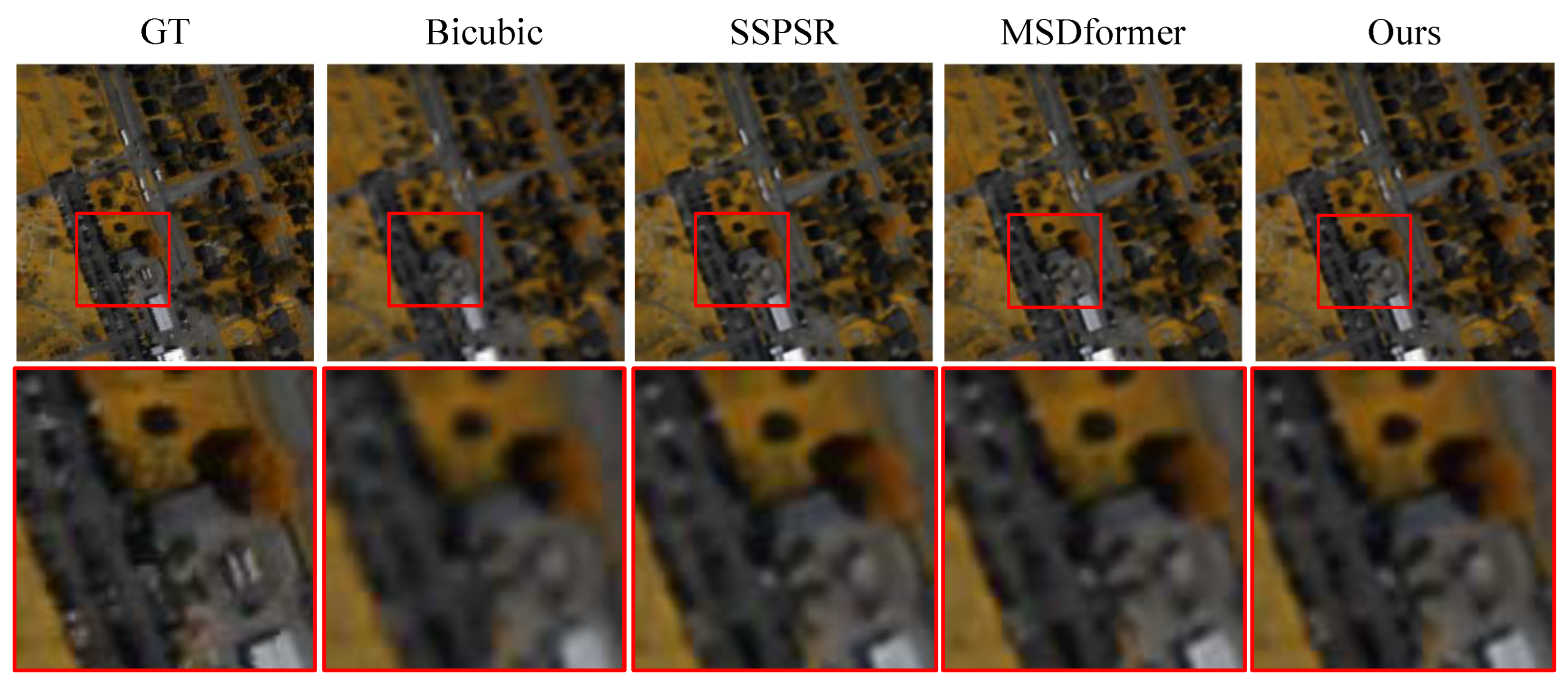
Figure 5 and Figure 6 showcase the visualization of HSI image reconstruction from the Chikusei test set at a scale factor of x4. We selected channels 31, 98, and 61 for RGB visualization to enhance visual interpretation. It is evident that while the bicubic method achieves SR of HSIs, it results in the blurriest edges and poorest reconstruction of smooth areas. SSPSR [14] and MSDformer [15] show better reconstruction, especially in terms of line details, but still exhibit flaws in detail restoration. Our SSAformer, however, achieves superior edge and detail restoration, clearly visible in the zoomed-in views marked by red boxes.

4.4.2. Experiments on the Houston Dataset

The Houston2018 dataset [52] comprises images of size 4172 × 1202 × 48. For testing, we simultaneously cropped four nonoverlapping HSIs of 256 × 256 × 48 at positions 1–256 pixels and 257–512 pixels in the vertical regions and similarly in the horizontal regions, resulting in eight nonoverlapping HSIs for testing. The width of the top area used for testing exceeding 256x4 was discarded. The remainder of the image was cropped into overlapping patches for training purposes, following the same preprocessing method as the Chikusei dataset [51] (with 10% of the training data randomly selected as a validation set).
Table 2 presents the quantitative results of various methods on the Houston test set across scale factors of ×2, ×4, and ×8 for six evaluation metrics. The best results are highlighted in bold, and the second-best are underlined. Our model outperformed other SOTA methods on all six evaluation metrics at the X2 scale factor. At the ×4 and ×8 scale factors, it exceeded other SOTA methods on five evaluation metrics, with the metrics not exceeded being only a few hundredths or thousandths less.
Figure 7 and Figure 8 demonstrate the qualitative results of HSI reconstruction from the Houston test set at a scale factor of x4. Specifically, we selected channels 29, 26, and 19 as the R-G-B channels for enhanced visualization. While the bicubic method could perform the SR task, its effectiveness is limited. SSPSR [14] and MSDformer [15] show significant improvements in reconstruction, but as observed in the red-boxed images, the SSAformer achieves better pixel-level restoration results.

4.4.3. Experiments on the Pavia Datasets

The Pavia Centre dataset [53] consists of images with dimensions of 1096 × 1096 × 102. Following the approach of [14,15], due to the presence of invalid areas, we cropped the informative region of the original scene to a size of 1096 × 715 × 102. The left side of the image was further segmented into four nonoverlapping HSIs of 224 × 224 × 102 for testing purposes. Any portion exceeding 224 × 4 in the vertical range on the left side was discarded. The remainder of the image was processed into overlapping training patches in the same manner as the Chikusei dataset [51], with 10% of the training data randomly selected as a validation set. Specifically, following the practice of [15], due to the smaller spatial dimensions of the Pavia dataset [53] relative to other datasets, for a scale factor of ×8 on the Pavia dataset [53], we used patches of 128 × 128 × 102 with an overlap of 64 pixels.
Table 3 shows the quantitative results of various methods on the Pavia test set across scale factors of ×2, ×4, and ×8 for six evaluation metrics. Our proposed SSAformer achieved better results than other SOTA methods across all scale factors. Given the smaller sample size of the Pavia dataset [53], this also indicates the robustness of our proposed method, demonstrating effective reconstruction capabilities across different data volumes, which is particularly relevant in scenarios where remote sensing data are scarce.
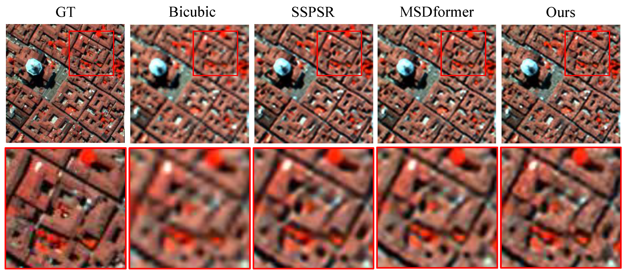
Figure 9 and Figure 10 showcase the qualitative results of HSI reconstruction from the Pavia test set at a scale factor of ×4. Specifically, we selected channels 100, 30, and 12 as the R-G-B channels for improved visualization. While the bicubic method is capable of performing the SR task, its effectiveness is limited. SSPSR [14] and MSDformer [15] show significant improvements in reconstruction, but the SSAformer achieves better recovery of some boundaries and pixel-level restoration effects.

4.5. Ablation Study

The effectiveness of spatial and spectral attention: In the SSAformer, we designed spatial and spectral attentions to separately learn the features from spatial and spectral dimensions. To validate the effectiveness of the proposed SAB, SEB, and SSAformer structures, we designed various SSAformer variants. By individually removing SAB or SEB, we denote these variants as “Ours w/o SAB” or “Ours w/o SEB,” respectively. As illustrated in Table 4, the performance of the model significantly decreases when using SAB or SEB alone. The probable reason is that each module specifically addresses either spatial or spectral information, and their concurrent action allows for information integration, facilitating comprehensive learning of spatial and spectral features in HSIs. When acting independently, there is a noticeable deficiency in the effective extraction of spatial or spectral information, failing to address the issues of long-range dependencies in spatial information or redundancy in spectral information.
The effectiveness of deformable convolution: To address the issue of channel information redundancy in HSIs, we introduced DC to extract information from each channel of HSIs adaptively. This is achieved through feature selection, implementing channel weighting to better extract information in the spectral dimension. To assess the effectiveness of DC within the SEB, we replaced the DC with standard convolution operations, denoted as w/o DC, with the experimental results shown in Table 4. All evaluation results are inferior to the original network with the DC module, indicating that DC benefits channel-wise feature extraction.
Analysis of the number of SSAGs: To extract global spatial–spectral information, we employ N SSAGs within our network. We investigated the impact of varying the number of SSAGs on the performance of hyperspectral SR, with the experimental results shown in Table 5. When a smaller number of modules (N = 3) is used, all quantitative metrics are at their worst, likely due to insufficient network depth to thoroughly learn spatial–spectral features. When the number of SSAGs is further set to 4 (N = 4), all quantitative metrics reach their optimum. However, when the number is larger, the SR performance starts to deteriorate since a deeper model requires more training data, leading to overfitting and poor generalization capability.

5. Conclusions

In this paper, we introduce the Spatial–Spectral Aggregation Transformer, termed SSAformer, for HSI SR. Specifically, we leverage specially designed spatial and spectral attention modules to efficiently extract and integrate spatial and spectral information in HSIs. The spatial attention module effectively models the long-range dependencies of spatial information, while the spectral attention module addresses the issue of channel redundancy in HSIs through channel weighting. Experiments on three public datasets demonstrate that our method can recover finer details and achieve minimal spectral distortion compared to SOTA methods, resulting in better reconstruction outcomes. Future work will focus on optimizing the network to make it lightweight and hardware-compatible. We also recognize the need to validate our findings across more varied real-world environments to fully assess the model’s applicability.

Author Contributions

H.W. and T.L. designed the model and implementation; H.W. and Q.Z. completed writing; H.W. and T.P. performed the experiments; Z.X. (Zhongjie Xu), X.C., Z.X. (Zhongyang Xing) and T.L. guided the research. All authors have read and agreed to the published version of the manuscript.

Funding

This research was supported by the High-level Talents Programme of National University of Defense Technology, and the National Natural Science Foundation of China (12204541).

Data Availability Statement

The original contributions presented in the study are included in the article, further inquiries can be directed to the corresponding author.

Acknowledgments

In this study, we extend our sincere gratitude to the Hyperspectral Image Analysis Laboratory and the National Center for Airborne Laser Mapping (NCALM) at the University of Houston for providing the unique multisensor optical geospatial data as part of the 2018 IEEE GRSS Data Fusion Contest.

Conflicts of Interest

The authors declare no conflicts of interest.

Abbreviations

HSIHyperspectral image
SRSuper-resolution
HRHigh resolution
LRLow resolution
CNNConvolutional neural network
SSAformerSpatial–Spectral Aggregation Transformer
DCDeformable convolution
SOTAState of the art
SSAGSpatial–spectral attention group
SSABSpatial–spectral attention block
MLPMultilayer perceptron
OCAOverlapping cross-attention
SABSpatial attention block
SEBSpectral attention block
PSNRPeak signal-to-noise ratio
SSIMStructural similarity index measure
SAMSpectral angle mapper
CCCross correlation
RMSERoot mean squared error
ERGASErreur relative global adimensionnelle de synthèse

References

  1. Shimoni, M.; Haelterman, R.; Perneel, C. Hypersectral Imaging for Military and Security Applications: Combining Myriad Processing and Sensing Techniques. IEEE Geosci. Remote Sens. Mag. 2019, 7, 101–117. [Google Scholar] [CrossRef]
  2. Zhang, Q.; Willmott, M.B. Review of Hyperspectral Imaging in Environmental Monitoring Progress and Applications. Acad. J. Sci. Technol. 2023, 6, 9–11. [Google Scholar] [CrossRef]
  3. Li, S.; Song, W.; Fang, L.; Chen, Y.; Ghamisi, P.; Benediktsson, J.A. Deep Learning for Hyperspectral Image Classification: An Overview. IEEE Trans. Geosci. Remote Sens. 2019, 57, 6690–6709. [Google Scholar] [CrossRef]
  4. Poojary, N.; D’Souza, H.; Puttaswamy, M.R.; Kumar, G.H. Automatic target detection in hyperspectral image processing: A review of algorithms. In Proceedings of the 2015 12th International Conference on Fuzzy Systems and Knowledge Discovery (FSKD), Zhangjiajie, China, 15–17 August 2015; pp. 1991–1996. [Google Scholar]
  5. Jiao, L.; Zhang, X.; Liu, X.; Liu, F.; Yang, S.; Ma, W.; Li, L.; Chen, P.; Feng, Z.; Guo, Y.; et al. Transformer Meets Remote Sensing Video Detection and Tracking: A Comprehensive Survey. IEEE J. Sel. Top. Appl. Earth Obs. Remote Sens. 2023, 16, 1–45. [Google Scholar] [CrossRef]
  6. Vivone, G. Multispectral and hyperspectral image fusion in remote sensing: A survey. Inf. Fusion 2022, 89, 405–417. [Google Scholar] [CrossRef]
  7. Wang, X.; Hu, Q.; Cheng, Y.; Ma, J. Hyperspectral Image Super-Resolution Meets Deep Learning: A Survey and Perspective. IEEE/CAA J. Autom. Sin. 2023, 10, 1668–1691. [Google Scholar] [CrossRef]
  8. Hu, Y.; Li, X.; Gu, Y.; Jacob, M. Hyperspectral Image Recovery Using Nonconvex Sparsity and Low-Rank Regularizations. IEEE Trans. Geosci. Remote Sens. 2020, 58, 532–545. [Google Scholar] [CrossRef]
  9. Bodrito, T.; Zouaoui, A.; Chanussot, J.; Mairal, J. A Trainable Spectral-Spatial Sparse Coding Model for Hyperspectral Image Restoration. arXiv 2021, arXiv:2111.09708. [Google Scholar]
  10. Zhang, M.; Sun, X.; Zhu, Q.; Zheng, G. A Survey of Hyperspectral Image Super-Resolution Technology. In Proceedings of the 2021 IEEE International Geoscience and Remote Sensing Symposium IGARSS, Brussels, Belgium, 11–16 July 2021; pp. 4476–4479. [Google Scholar]
  11. Chen, C.; Wang, Y.; Zhang, N.; Zhang, Y.; Zhao, Z. A Review of Hyperspectral Image Super-Resolution Based on Deep Learning. Remote. Sens. 2023, 15, 2853. [Google Scholar] [CrossRef]
  12. Dong, C.; Loy, C.C.; He, K.; Tang, X. Learning a Deep Convolutional Network for Image Super-Resolution. In Proceedings of the European Conference on Computer Vision, Zurich, Switzerland, 6–12 September 2014; Springer: Cham, Switzerland, 2014. [Google Scholar]
  13. Zhang, Y.; Li, K.; Li, K.; Wang, L.; Zhong, B.; Fu, Y.R. Image Super-Resolution Using Very Deep Residual Channel Attention Networks. arXiv 2018, arXiv:1807.02758. [Google Scholar]
  14. Jiang, J.; Sun, H.; Liu, X.; Ma, J. Learning Spatial-Spectral Prior for Super-Resolution of Hyperspectral Imagery. IEEE Trans. Comput. Imaging 2020, 6, 1082–1096. [Google Scholar] [CrossRef]
  15. Chen, S.; Zhang, L.; Zhang, L. MSDformer: Multiscale Deformable Transformer for Hyperspectral Image Super-Resolution. IEEE Trans. Geosci. Remote Sens. 2023, 61, 1–14. [Google Scholar] [CrossRef]
  16. Li, J.; Fang, F.; Mei, K.; Zhang, G. Multi-scale Residual Network for Image Super-Resolution. In Proceedings of the European Conference on Computer Vision, Munich, Germany, 8–14 September 2018. [Google Scholar]
  17. Lu, T.; Wang, J.; Zhang, Y.; Wang, Z.; Jiang, J. Satellite Image Super-Resolution via Multi-Scale Residual Deep Neural Network. Remote Sens. 2019, 11, 1588. [Google Scholar] [CrossRef]
  18. Wang, Y.; Shao, Z.; Lu, T.; Wu, C.; Wang, J. Remote Sensing Image Super-Resolution via Multiscale Enhancement Network. IEEE Geosci. Remote Sens. Lett. 2023, 20, 5000905. [Google Scholar] [CrossRef]
  19. Mei, S.; Yuan, X.; Ji, J.; Zhang, Y.; Wan, S.; Du, Q. Hyperspectral Image Spatial Super-Resolution via 3D Full Convolutional Neural Network. Remote Sens. 2017, 9, 1139. [Google Scholar] [CrossRef]
  20. Li, Q.; Wang, Q.; Li, X. Mixed 2D/3D Convolutional Network for Hyperspectral Image Super-Resolution. Remote Sens. 2020, 12, 1660. [Google Scholar] [CrossRef]
  21. Aiazzi, B.; Alparone, L.; Baronti, S.; Garzelli, A.; Selva, M. MTF-tailored Multiscale Fusion of High-resolution MS and Pan Imagery. Photogramm. Eng. Remote Sens. 2006, 72, 591–596. [Google Scholar] [CrossRef]
  22. Akhtar, N.; Shafait, F.; Mian, A. Bayesian sparse representation for hyperspectral image super resolution. In Proceedings of the 2015 IEEE Conference on Computer Vision and Pattern Recognition (CVPR), Boston, MA, USA, 1–7 June 2015; pp. 3631–3640. [Google Scholar]
  23. Sun, W.; Liu, C.; Li, J.; Lai, Y.M.; Li, W. Low-rank and sparse matrix decomposition-based anomaly detection for hyperspectral imagery. J. Appl. Remote Sens. 2014, 8, 083641. [Google Scholar] [CrossRef]
  24. Wang, Y.; Peng, J.; Zhao, Q.; Leung, Y.; Zhao, X.L.; Meng, D. Hyperspectral Image Restoration Via Total Variation Regularized Low-Rank Tensor Decomposition. IEEE J. Sel. Top. Appl. Earth Obs. Remote Sens. 2018, 11, 1227–1243. [Google Scholar] [CrossRef]
  25. Li, Y.; Zhang, L.; Tian, C.; Ding, C.; Zhang, Y.; Wei, W. Hyperspectral image super-resolution extending: An effective fusion based method without knowing the spatial transformation matrix. In Proceedings of the 2017 IEEE International Conference on Multimedia and Expo (ICME), Hong Kong, China, 10–14 July 2017; pp. 1117–1122. [Google Scholar]
  26. Bauschke, H.H.; Borwein, J.M. On Projection Algorithms for Solving Convex Feasibility Problems. SIAM Rev. 1996, 38, 367–426. [Google Scholar] [CrossRef]
  27. Liu, C.; Fan, Z.; Zhang, G. GJTD-LR: A Trainable Grouped Joint Tensor Dictionary With Low-Rank Prior for Single Hyperspectral Image Super-Resolution. IEEE Trans. Geosci. Remote Sens. 2022, 60, 5537617. [Google Scholar] [CrossRef]
  28. Xie, W.; Jia, X.; Li, Y.; Lei, J. Hyperspectral Image Super-Resolution Using Deep Feature Matrix Factorization. IEEE Trans. Geosci. Remote Sens. 2019, 57, 6055–6067. [Google Scholar] [CrossRef]
  29. Akgun, T.; Altunbasak, Y.; Mersereau, R. Super-resolution reconstruction of hyperspectral images. IEEE Trans. Image Process. 2005, 14, 1860–1875. [Google Scholar] [CrossRef]
  30. Yokoya, N.; Yairi, T.; Iwasaki, A. Coupled Nonnegative Matrix Factorization Unmixing for Hyperspectral and Multispectral Data Fusion. IEEE Trans. Geosci. Remote Sens. 2012, 50, 528–537. [Google Scholar] [CrossRef]
  31. He, W.; Chen, Y.; Yokoya, N.; Li, C.; Zhao, Q. Hyperspectral Super-Resolution via Coupled Tensor Ring Factorization. Pattern Recognit. 2020, 122, 108280. [Google Scholar] [CrossRef]
  32. Dong, C.; Loy, C.C.; He, K.; Tang, X. Image Super-Resolution Using Deep Convolutional Networks. IEEE Trans. Pattern Anal. Mach. Intell. 2016, 38, 295–307. [Google Scholar] [CrossRef]
  33. Yuan, Y.; Zheng, X.; Lu, X. Hyperspectral Image Superresolution by Transfer Learning. IEEE J. Sel. Top. Appl. Earth Obs. Remote Sens. 2017, 10, 1963–1974. [Google Scholar] [CrossRef]
  34. Li, Y.; Zhang, L.; Dingl, C.; Wei, W.; Zhang, Y. Single Hyperspectral Image Super-Resolution with Grouped Deep Recursive Residual Network. In Proceedings of the 2018 IEEE Fourth International Conference on Multimedia Big Data (BigMM), Xi’an, China, 13–16 September 2018; pp. 1–4. [Google Scholar]
  35. Jia, J.; Ji, L.; Zhao, Y.; Geng, X. Hyperspectral image super-resolution with spectral–spatial network. Int. J. Remote Sens. 2018, 39, 7806–7829. [Google Scholar] [CrossRef]
  36. Brown, T.B.; Mann, B.; Ryder, N.; Subbiah, M.; Kaplan, J.; Dhariwal, P.; Neelakantan, A.; Shyam, P.; Sastry, G.; Askell, A.; et al. Language Models are Few-Shot Learners. arXiv 2020, arXiv:2005.14165. [Google Scholar]
  37. Devlin, J.; Chang, M.W.; Lee, K.; Toutanova, K. BERT: Pre-training of Deep Bidirectional Transformers for Language Understanding. In Proceedings of the North American Chapter of the Association for Computational Linguistics, Minneapolis, MN, USA, 3–5 June 2019. [Google Scholar]
  38. Vaswani, A.; Shazeer, N.M.; Parmar, N.; Uszkoreit, J.; Jones, L.; Gomez, A.N.; Kaiser, L.; Polosukhin, I. Attention is All you Need. In Proceedings of the Neural Information Processing Systems, Long Beach, CA, USA, 4–9 December 2017. [Google Scholar]
  39. Wolf, T.; Debut, L.; Sanh, V.; Chaumond, J.; Delangue, C.; Moi, A.; Cistac, P.; Rault, T.; Louf, R.; Funtowicz, M.; et al. Transformers: State-of-the-Art Natural Language Processing. In Proceedings of the Conference on Empirical Methods in Natural Language Processing, Online, 29 October 2019. [Google Scholar]
  40. Liu, Y.; Hu, J.; Kang, X.; Luo, J.; Fan, S. Interactformer: Interactive Transformer and CNN for Hyperspectral Image Super-Resolution. IEEE Trans. Geosci. Remote Sens. 2022, 60, 5531715. [Google Scholar] [CrossRef]
  41. Hu, J.; Liu, Y.; Kang, X.; Fan, S. Multilevel Progressive Network With Nonlocal Channel Attention for Hyperspectral Image Super-Resolution. IEEE Trans. Geosci. Remote Sens. 2022, 60, 5543714. [Google Scholar] [CrossRef]
  42. Wu, Y.; Cao, R.; Hu, Y.; Wang, J.; Li, K. Combining global receptive field and spatial spectral information for single-image hyperspectral super-resolution. Neurocomputing 2023, 542, 126277. [Google Scholar] [CrossRef]
  43. Geng, Z.; Guo, M.H.; Chen, H.; Li, X.; Wei, K.; Lin, Z. Is Attention Better Than Matrix Decomposition? arXiv 2021, arXiv:2109.04553. [Google Scholar]
  44. Katharopoulos, A.; Vyas, A.; Pappas, N.; Fleuret, F. Transformers are RNNs: Fast Autoregressive Transformers with Linear Attention. In Proceedings of the International Conference on Machine Learning, Virtual, 13–18 July 2020. [Google Scholar]
  45. Zhang, M.; Zhang, C.; Zhang, Q.; Guo, J.; Gao, X.; Zhang, J. ESSAformer: Efficient Transformer for Hyperspectral Image Super-resolution. In Proceedings of the 2023 IEEE/CVF International Conference on Computer Vision (ICCV), Paris, France, 22–29 October 2023; pp. 23016–23027. [Google Scholar]
  46. Dai, J.; Qi, H.; Xiong, Y.; Li, Y.; Zhang, G.; Hu, H.; Wei, Y. Deformable Convolutional Networks. In Proceedings of the 2017 IEEE International Conference on Computer Vision (ICCV), Venice, Italy, 22–29 October 2017; pp. 764–773. [Google Scholar]
  47. Liu, Z.; Lin, Y.; Cao, Y.; Hu, H.; Wei, Y.; Zhang, Z.; Lin, S.; Guo, B. Swin Transformer: Hierarchical Vision Transformer using Shifted Windows. In Proceedings of the 2021 IEEE/CVF International Conference on Computer Vision (ICCV), Virtual, 11–17 October 2021; pp. 9992–10002. [Google Scholar]
  48. Chen, X.; Wang, X.; Zhang, W.; Kong, X.; Qiao, Y.; Zhou, J.; Dong, C. HAT: Hybrid Attention Transformer for Image Restoration. arXiv 2023, arXiv:2309.05239. [Google Scholar]
  49. Lim, B.; Son, S.; Kim, H.; Nah, S.; Lee, K.M. Enhanced Deep Residual Networks for Single Image Super-Resolution. In Proceedings of the 2017 IEEE Conference on Computer Vision and Pattern Recognition Workshops (CVPRW), Honolulu, HI, USA, 21–26 July 2017; pp. 1132–1140. [Google Scholar]
  50. Wang, X.; Ma, J.; Jiang, J. Hyperspectral Image Super-Resolution via Recurrent Feedback Embedding and Spatial–Spectral Consistency Regularization. IEEE Trans. Geosci. Remote Sens. 2022, 60, 1–13. [Google Scholar] [CrossRef]
  51. Yokoya, N.; Iwasaki, A. Airborne Hyperspectral Data over Chikusei; The University of Tokyo: Tokyo, Japan, 2016. [Google Scholar]
  52. Xu, Y.; Du, B.; Zhang, L.; Cerra, D.; Pato, M.; Carmona, E.; Prasad, S.; Yokoya, N.; Hänsch, R.; Le Saux, B. Advanced Multi-Sensor Optical Remote Sensing for Urban Land Use and Land Cover Classification: Outcome of the 2018 IEEE GRSS Data Fusion Contest. IEEE J. Sel. Top. Appl. Earth Obs. Remote Sens. 2019, 12, 1709–1724. [Google Scholar] [CrossRef]
  53. Huang, X.; Zhang, L. A comparative study of spatial approaches for urban mapping using hyperspectral ROSIS images over Pavia City, northern Italy. Int. J. Remote Sens. 2009, 30, 3205–3221. [Google Scholar] [CrossRef]
  54. Wang, Z.; Bovik, A.; Sheikh, H.; Simoncelli, E. Image quality assessment: From error visibility to structural similarity. IEEE Trans. Image Process. 2004, 13, 600–612. [Google Scholar] [CrossRef]
  55. Yuhas, R.H.; Goetz, A.F.H.; Boardman, J.W. Discrimination among Semi-Arid Landscape Endmembers Using the Spectral Angle Mapper (SAM) Algorithm; NTRS: Chicago, IL, USA, 1992. [Google Scholar]
  56. Loncan, L.; de Almeida, L.B.; Bioucas-Dias, J.M.; Briottet, X.; Chanussot, J.; Dobigeon, N.; Fabre, S.; Liao, W.; Licciardi, G.A.; Simões, M.; et al. Hyperspectral Pansharpening: A Review. IEEE Geosci. Remote Sens. Mag. 2015, 3, 27–46. [Google Scholar] [CrossRef]
  57. Wald, L. Data Fusion. Definitions and Architectures—Fusion of Images of Different Spatial Resolutions; Presses des MINES: Paris, France, 2002. [Google Scholar]
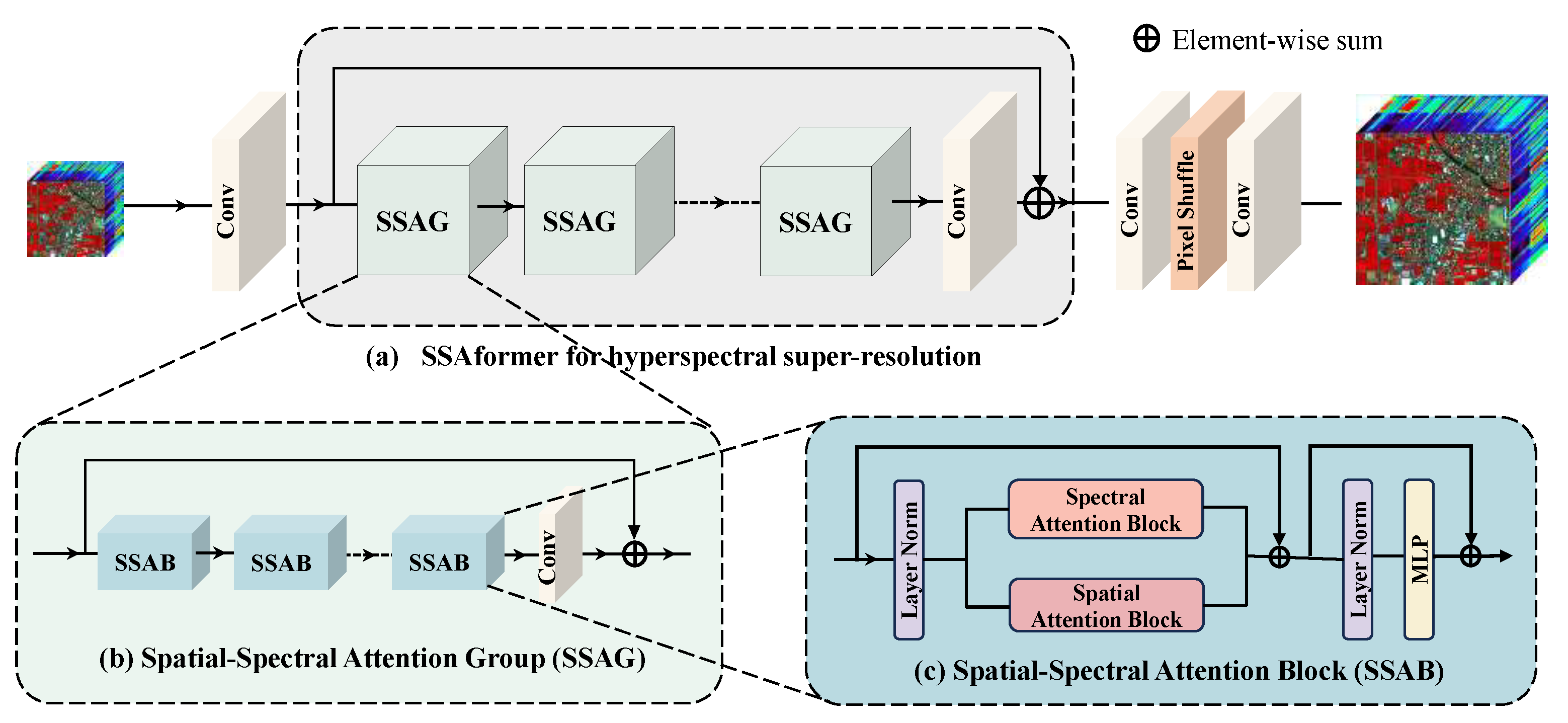
Figure 1. The overall architecture of SSAformer and the structure of the SSAGs and SSABs: (a) representing the main pipeline of SSAformer operation, wherein the detailed structure of the SSAGs and SSABs is elucidated in (b,c).
Remotesensing 16 01766 g001
Figure 2. Structure of the designed spectral attention block.
Remotesensing 16 01766 g002
Figure 3. Sample point variation of deformable convolutional operations (D Conv).
Remotesensing 16 01766 g003
Figure 4. Structure of the designed spatial attention block.
Remotesensing 16 01766 g004
Figure 5. Reconstructed test HSIs in the Chikusei dataset with spectral bands 31-98-61 as R-G-B at scale factor ×4. From left to right, ground truth, then results of bicubic, SSPSR [14], MSDformer [15], and the proposed SSAformer method.
Remotesensing 16 01766 g005
Figure 6. Error maps of the test HSIs in the Chikusei dataset at the scale factor ×4.
Remotesensing 16 01766 g006
Figure 7. Reconstructed test HSIs in the Houston dataset with spectral bands 29-26-19 as R-G-B at scale factor ×4. From left to right, ground truth, then results of bicubic, SSPSR [14], MSDformer [15], and the proposed SSAformer method.
Remotesensing 16 01766 g007
Figure 8. Error maps of the test HSIs in the Houston dataset at the scale factor ×4.
Remotesensing 16 01766 g008
Figure 9. Reconstructed test HSIs in the Pavia dataset with spectral bands 100-30-12 as R-G-B at scale factor ×4. From left to right, ground truth, then results of bicubic, SSPSR [14], MSDformer [15], and the proposed SSAformer method.
Remotesensing 16 01766 g009
Figure 10. Error maps of the test HSIs in the Pavia dataset at the scale factor ×4.
Remotesensing 16 01766 g010
Table 1. Quantitative evaluation of different HSI SR methods on the Chikusei dataset. The best and second-best results are bolded and underlined, respectively.
Method ScalePSNR↑SSIM↑SAM↓CC↑RMSE↓ERGAS↓
Bicubic × 2 43.21250.97211.78800.97810.00823.5981
3DFCNN [19] × 2 45.44770.98281.55500.98540.00642.9235
GDRRN [34] × 2 46.42860.98691.39110.98850.00562.6049
SSPSR [14] × 2 47.40730.98931.20350.99060.00512.3177
MSDformer [15] × 2 47.08680.98821.18430.98990.00542.3359
Ours × 2 47.59840.98991.17100.99080.00492.2926
Bicubic × 4 37.63770.89543.40400.92120.01566.7564
3DFCNN [19] × 4 38.12210.90793.39270.92760.01476.4453
GDRRN [34] × 4 39.08640.92653.05360.94210.01305.7972
SSPSR [14] × 4 39.55650.93312.57010.94820.01255.4019
MSDformer [15] × 4 39.53230.93442.53540.94790.01265.4152
Ours × 4 39.69550.93702.51220.94900.01225.3754
Bicubic × 8 34.50490.80695.04360.83140.02249.6975
3DFCNN [19] × 8 34.72740.81424.95140.83790.02189.4706
GDRRN [34] × 8 34.73950.81995.09670.83810.02139.6464
SSPSR [14] × 8 35.16430.82994.69110.85600.02069.0504
MSDformer [15] × 8 35.27420.83574.49710.85940.02078.7425
Ours × 8 35.32410.84024.35720.85990.02018.8235
Table 2. Quantitative evaluation of different HSI SR methods on the Houston dataset. The best and second-best results are bolded and underlined, respectively.
MethodScalePSNR↑SSIM↑SAM↓CC↑RMSE↓ERGAS↓
Bicubic × 2 49.47350.99151.27070.99400.00401.3755
3DFCNN [19] × 2 50.79390.99411.21680.99490.00341.1722
GDRRN [34] × 2 51.52050.99491.12410.99570.00311.0723
SSPSR [14] × 2 52.50610.99581.01010.99650.00280.9608
MSDformer [15] × 2 51.92650.99521.06000.99630.00301.0223
Ours × 2 52.59050.99600.96680.99680.00270.9475
Bicubic × 4 43.02720.96132.54530.97410.00862.9085
3DFCNN [19] × 4 43.26800.96692.61280.96610.00792.8698
GDRRN [34] × 4 44.29640.97302.53470.97600.00692.4700
SSPSR [14] × 4 45.59870.97791.88280.98500.00632.1377
MSDformer [15] × 4 45.64120.97821.85820.98520.00622.1279
Ours × 4 45.64570.97881.85530.98500.00612.1141
Bicubic × 8 38.10830.89874.67040.91770.01525.1229
3DFCNN [19] × 8 38.01520.90304.70850.90930.01465.0865
GDRRN [34] × 8 38.25920.90854.90450.91380.01404.9135
SSPSR [14] × 8 39.28440.91644.26730.93460.01304.4212
MSDformer [15] × 8 39.26830.91654.05150.93540.01314.4383
Ours × 8 39.23200.91873.91540.94390.01294.4146
Table 3. Quantitative evaluation of different HSI SR methods on the Pavia dataset. The best and second-best results are bolded and underlined, respectively.
MethodScalePSNR↑SSIM↑SAM↓CC↑RMSE↓ERGAS↓
Bicubic × 2 32.05830.91394.54190.94910.02564.1526
3DFCNN [19] × 2 33.37970.93694.61730.95960.02193.6197
GDRRN [34] × 2 33.89490.94284.70060.96410.02063.4179
SSPSR [14] × 2 34.87240.95254.01430.97060.01853.0734
MSDformer [15] × 2 35.44000.96013.50410.97460.01732.9166
Ours × 2 35.73170.96083.50480.97600.01672.8263
Bicubic × 4 27.32220.71516.36600.84930.04517.0292
3DFCNN [19] × 4 27.71030.75466.56700.85820.04296.7438
GDRRN [34] × 4 27.96020.76957.16700.86640.04146.5732
SSPSR [14] × 4 28.47570.79115.78670.88480.03926.2282
MSDformer [15] × 4 28.50320.79295.79070.88530.03906.2197
Ours × 4 28.61990.79885.73690.88830.03846.1420
Bicubic × 8 24.37140.45317.89030.67630.06469.8142
3DFCNN [19] × 8 24.31730.45328.15560.66750.06479.8779
GDRRN [34] × 8 24.54680.47778.48730.68420.06309.6256
SSPSR [14] × 8 24.66410.49428.30480.69460.06209.4980
MSDformer [15] × 8 24.84180.50977.80210.71260.06089.4031
Ours × 8 24.84680.51117.67290.71340.06079.3920
Table 4. Ablation experiments of some variants of the proposed method over the Pavia testing dataset at scale factor ×4. Bold represents the best.
VariantParams. ( × 10 6 )PSNR↑SSIM↑SAM↓CC↑RMSE↓ERGAS↓
w/o SAB13.186627.97110.76696.20270.86960.04146.6139
w/o SEB17.741727.96440.76636.18480.86940.04156.6173
w/o DC22.469427.96850.76656.17960.86940.04156.6157
Ours22.585628.61990.79885.73690.88830.03846.1420
Table 5. Quantitative comparisons of the number of SSAGs over the Pavia testing dataset at scale factor ×4. Bold represents the best.
Number (N)Params. ( × 10 6 )PSNR↑SSIM↑SAM↓CC↑RMSE↓ERGAS↓
N = 317.168227.92070.76476.30970.86810.04176.6536
N = 422.585628.61990.79885.73690.88830.03846.1420
N = 528.003028.02140.76956.10530.87120.04126.5752
N = 633.420428.54230.79415.87710.88610.03876.2022
Disclaimer/Publisher’s Note: The statements, opinions and data contained in all publications are solely those of the individual author(s) and contributor(s) and not of MDPI and/or the editor(s). MDPI and/or the editor(s) disclaim responsibility for any injury to people or property resulting from any ideas, methods, instructions or products referred to in the content.