A Cross-Channel Dense Connection and Multi-Scale Dual Aggregated Attention Network for Hyperspectral Image Classification

Abstract

Hyperspectral image classification (HSIC) is one of the most important research topics in the field of remote sensing. However, it is difficult to label hyperspectral data, which limits the improvement of classification performance of hyperspectral images in the case of small samples. To alleviate this problem, in this paper, a dual-branch network which combines cross-channel dense connection and multi-scale dual aggregated attention (CDC_MDAA) is proposed. On the spatial branch, a cross-channel dense connections (CDC) module is designed. The CDC can effectively combine cross-channel convolution with dense connections to extract the deep spatial features of HSIs. Then, a spatial multi-scale dual aggregated attention module (SPA_MDAA) is constructed. The SPA_MDAA adopts dual autocorrelation for attention modeling to strengthen the differences between features and enhance the ability to pay attention to important features. On the spectral branch, a spectral multi-scale dual aggregated attention module (SPE_MDAA) is designed to capture important spectral features. Finally, the spatial spectral features are fused, and the classification results are obtained. The experimental results show that the classification performance of the proposed method is superior to some state-of-the-art methods in small samples and has good generalization.

1. Introduction

Hyperspectral images (HSIs) have been used in a variety of fields as remote sensing technology has advanced [1]. Almost all walks of life are involved, from national military security to agricultural crop growth; from the detection of water resources to the monitoring of mountain fire forestry; from atmospheric exploration to geological survey; from the medical industry to mineral resources [2,3,4,5]. These applications, however, are intrinsically closely related to hyperspectral image classification (HSIC) technology [6].

In the early days, the methods used for HSIC were mainly classical machine learning algorithms. For example, a K-nearest neighbor classifier [7] was constructed by Samaniego L. A maximum likelihood classifier [8] was designed by Ediriwickrema J. A method of Rogers regression [9] was proposed by Foody G M. However, the classification performance of these methods is relatively poor when the number of samples is small and the data dimension of HSI is too high. To this end, a principal component analysis (PCA) method [10] was proposed by Prasad S. PCA is used to map high-dimensional data to low-dimensional space, lower the dimension of HSI, and keep the basic feature information of HSI. The information of the spatial dimension was overlooked by the early HSIC, which only took into account the information of the spectral dimension. However, HSI is obtained by simultaneously imaging the target area with multiple continuously subdivided bands. This means that a lot of spectral information and spatial information are contained by HSIs [11]. Therefore, the spectral information and spatial information of HSI need to be extracted simultaneously when the HSI is classified. Thereupon, the HSIC method based on the combination of spatial spectral features was proposed [12,13,14,15,16]. Among them, [12] utilizes a hybrid framework of principal component analysis (PCA), finite element method based on hierarchical learning, and logistic regression (LR) to extract spectral spatial features to achieve high classification accuracy [13]. The sparse multinomial logistic regression (SMLR) classifier is used to learn spectral information, and the spatial features are modeled by spatially adaptive total variation (SpATV) regularization. In [14], a deep learning (DL) framework combining PCA, DL, and LR is proposed, which can fuse spatial and spectral features to significantly improve the classification performance of HSIs. In [15], the author reduces spectral loss through spectral spatial weighted modulation and spectral compensation. The effectiveness of the method was verified through classification results. In [16], a multi-scale low rank decomposition algorithm is used to extract multi-scale spatial features, and a Landmark-neighborhood preserving embedding algorithm is used to fuse spatial and spectral features. In addition, the classification performance of the network largely depends on its feature extraction ability [17,18,19,20,21,22]. However, the feature extraction of the network is seriously disturbed by the complex and diverse distribution of ground objects in HSI. It is difficult to find a specific feature extraction method suitable for all HSIs. The emergence of convolutional neural networks (CNNs) [23,24] brings great convenience to feature extraction.

This has made CNN popular with researchers in the field of HSIC, and some excellent classification methods have also been proposed. For example, a classification method of the three-dimensional convolutional neural network (3D-CNN) was proposed by Chen [25]. 3D-CNN can extract deep spatial and spectral information at the same time and has achieved good classification results. In order to mine deeper features, it is often necessary to extract deeper features by overlapping multi-layer convolutions. However, if the convolution layer of the network is too deep, it will lead to the problem of gradient explosion and gradient disappearance. This will make the network training difficult to converge, over-fit, and may even lead to network collapse. In addition, blind stacking of convolutions will inevitably bring huge parameter quantities. This will cause the network training speed to become extremely slow and also bring a great burden to the computer hardware equipment. The emergence of deep residual networks (resnet) and dense connected networks (DenseNet) has greatly alleviated this problem [26,27,28,29,30,31,32,33]. As such, a multi-scale dense network (MSDN) was proposed [34], which reduced the loss of information in feature engineering and extracted more abundant fine features at low cost. After that, a multi-layer fusion dense network (MFDN) was proposed by Li [35] to extract features in different scenarios through multi-scale dense connections and fuse them. However, the distribution of ground objects in the dataset used for HSIC is chaotic, which brings a great test to the classification network. This also makes feature extraction crucial in classification tasks. When the number of samples is small, if more key features cannot be obtained, it is difficult to accurately predict all categories in classification prediction. Therefore, unified multi-scale learning (UML) was proposed by Wang [36]. UML uses multi-scale channel shuffling to shuffle channel features of different sizes, which can effectively extract more different features. Nevertheless, in the HSI dataset with extremely few sample labels, it is still a difficult point to effectively improve the classification performance of the model.

Recently, in order to alleviate the problem of sample scarcity, an attention mechanism was proposed [37,38,39,40]. An attention mechanism is a mechanism that emphasizes the area of interest and suppresses the irrelevant background area in the way of “dynamic weighting”. An attention-assisted CNN model [41] was proposed by Hang. Hang combines attention with CNN in parallel to extract more discriminative spatial spectral features. However, convolution is not robust to the rotation of spatial position, which will affect the improvement of classification accuracy. Therefore, a rotation-invariant attention network (RIAN) and a cross-attention-spectrum-spatial network (CASSN) have been proposed successively [42,43]. RIAN restrains the interference of position rotation on classification by correcting attention in space, while CASSN uses the interaction of cross- spatial attention to mitigate the impact of position rotation. In addition, Ma et al. designed a double-branch multi-attention network (DBMA) by combining a multi-branch structure with attention [44] and achieved good classification performance. A double-branch dual-attention network (DBDA) [45] was proposed by Li. DBDA captures the spatial information and spectral information of HSI through double branches and classifies them with attention. In the past two years, a transformer model combining self-attention has been proposed. In [46], a hyperspectral image transformer in transformer (HSI-TNT) method was proposed. In this method, two transformer deep networks were used to fuse local and global features, and the effectiveness of the method was finally demonstrated through a large number of experiments.

However, in the case of small samples, improving the feature extraction ability of the network and strengthening the ability to pay attention to spatial spectral information to achieve high-precision classification is still a major difficulty in HSIC. In order to alleviate this problem and further improve the classification performance in the HSIC with extremely scarce sample labels, a HSIC method of cross-channel dense connections and multi-scale dual aggregated attention (CDC_MDAA) with double branches was proposed in this paper. First, on the spatial branch, a cross-channel dense connection (CDC) is proposed. CDC realizes the interactive fusion of channel information and makes use of dense connection to multiplexing spatial features multiple times to extract the depth spatial features of HSIs. Then, in order to capture the key spatial spectral features, a dual aggregated attention (DAA) method is proposed. In particular, the DAA is divided into a spatial dual aggregated attention module (SPA_DAA) and a spectral dual aggregated attention module (SPE_DAA). SPA_ DAA and SPE_ DAA can focus on the extracted spatial features and spectral features, respectively, and enhance the difference of features to capture important features conducive to classification. After a lot of experiments, compared with other mainstream methods, CDC_ MDAA can achieve optimal classification performance on different data sets.

The main contributions of this paper include the following four parts:

(1)

In this article, a cross channel dense connection and multi-scale dual aggregated attention network (CDC_MDAA) is proposed to alleviate the small sample problem, and extensive experiments have shown that the proposed method is superior to some state-of-the-art methods in small samples.

(2)

A CDC module is proposed, which combines cross-channel convolution with dense connection to effectively extract the spatial features of HSIs. The CDC realizes the interactive fusion of channel information and introduces dense connections. The same feature can be multiplexed multiple times, the loss of information in the feature extraction process can be reduced, and too many parameters are avoided.

(3)

A DAA module is constructed. The DAA uses dual autocorrelation for attention modeling, which can strengthen the difference between features to enhance the ability to pay attention to important features. In addition, enhanced normalization is proposed to further highlight important features.

(4)

A multi-scale head strategy is proposed for the DAA mechanism. It can increase the receptive field and obtain the attention value of multiple features to enhance the attention ability.

The rest of this paper is organized as follows. Section 2 is divided into four parts, which, respectively, introduce the overall architecture of CDC_MDAA, CDC, DAA, and multi-scale header strategies. In Section 3, the data sets, experimental parameters, model framework setting, and experimental analysis are discussed. Finally, in Section 4, conclusions are given.

2. Methods

In this paper, a CDC_MDAA is proposed for HSI classification. The CDC_MDAA is mainly composed of three parts. The first part is the CDC module and residual connection module for feature extraction. The second part is the DAA mechanism, which enhances important features by dynamic weighting. In the third part, a multi-scale head strategy is designed based on DAA to expand the receptive field and enhance the ability of attention to features.

2.1. The Overall Framework of CDC_MDAA

The CDC_MDAA proposed in this paper is composed of a CDC module, a residual connection, DAA, global average pooling (GAP), and a full connection (FC) layer, as shown in Figure 1. The CDC_ MDAA is a spatial-spectral association dual-branch network composed of a spatial branch and a spectral branch. On the spatial branch, the spatial features of HSI are extracted by the CDC module. After obtaining the spatial feature maps, they are processed by a nonlinear deformation module to reduce the dimension and then input into the spatial aggregated attention mechanism. The spatial aggregated attention mechanism connects two SPA_MDAA (composed of the multi-scale header strategy and SPA_DAA) modules by skipping connection to strengthen the attention ability. Similarly, in the spectral branch, the spectral features are extracted by the residual connection module and then the extracted features are introduced into the proposed spectral aggregated attention mechanism. The spectral aggregated attention mechanism is composed of two SPE_MDAA (composed of the multi-scale header strategy and SPE_DAA) modules, which also adopt skipping connection. Then, spectral branch and spatial branch are fused, and then processed through a convolution layer and GAP. Finally, it is passed into the FC and the classification results are obtained.

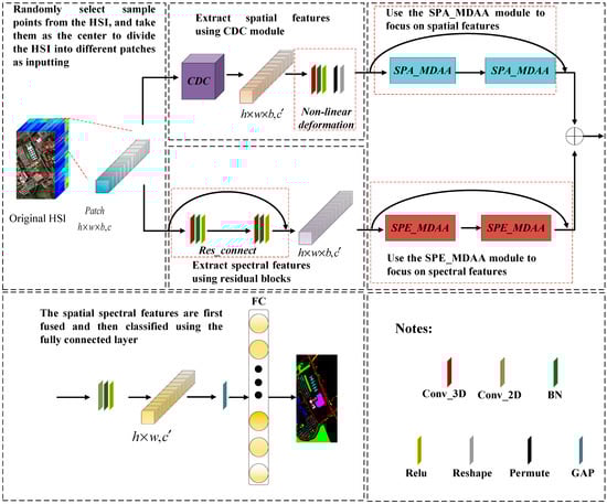
Figure 1. The overall structure of CDC_MDAA.

2.2. The CDC Module

In this paper, the CDC module is proposed by combining cross-channel convolution and dense connection. As shown in Figure 2, the convolution kernel of size $1\times 1\times 1$ is adopted at the beginning, which greatly reduces the number of parameters of the model and limits the number of channels, which facilitates the subsequent feature extraction. Then convolution kernel of size $3\times 3\times 1$ is used for the interactive fusion of channel information. This process can be described as

$$x_1=\mathrm{Re}lu\left(BN\left(F_1\left(x;w_{F_1}\right)\right)\right)x\in {ℝ}^{h\times w\times b,c},x_1\in {ℝ}^{h\times w\times b,c_1}$$

(1)

$$x_2=\mathrm{Re}lu\left(BN\left(F_2\left(x;w_{F_2}\right)\right)\right)x\in {ℝ}^{h\times w\times b,c},x_2\in {ℝ}^{h\times w\times b,c_2}$$

(2)

$$x_3=\mathrm{Re}lu\left(BN\left(F_3\left(x;w_{F_3}\right)\right)\right)x\in {ℝ}^{h\times w\times b,c},x_3\in {ℝ}^{h\times w\times b,c_3}$$

(3)

$$x^{\prime }=Ca{t}_c\left(f_1\left(x_1;w_{f_1}\right);f_2\left(x_2;w_{f_2}\right);f_3\left(x_3;w_{f_3}\right)\right)x^{\prime }\in {ℝ}^{h\times w\times b,c^{\prime }}$$

(4)

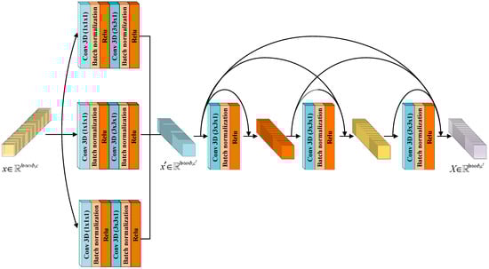
Figure 2. The CDC module.

Among them, $F_1(·)$, $F_2(·)$, and $F_3(·)$, in turn, represent the pointwise convolutionwith the number of output channels being 12, 24, and 36. $BN(·)$ is batch normalization and $\mathrm{Re}lu(·)$ is activation function. $f_1(·)$, $f_2(·)$, and $f_3(·)$ represent three composite functions that integrate convolution, batch normalization, and activation functions. The difference is that the input channel sizes of their convolution kernel are 12, 24, and 36, in order. $Ca{t}_c(·)$ refers to the operation of connecting according to the channel dimension. In addition, $c$ is the number of channels of $x$.$b$,$h$, and $w$, in turn, representing the band, length, and width of $x$. $c_1$, $c_2$, and $c_3$ are the number of channels with sizes of 12, 24, and 36, respectively. $c^{\prime }$ is the number of channels with size 64.

Then, the dense connection is integrated into the CDC module. During back propagation, each layer will receive gradient signals of all layers following it. Therefore, as the network depth increases, the gradient near the input layer will become smaller and smaller. This will cause the gradient of the network to disappear. During back propagation, gradient signals of all layers can be used repeatedly by dense connection, which to some extent alleviates the problem of gradient dissipation during training. In addition, a large number of features are reused during forward propagation, so that a large number of features can be generated even with a small number of convolution cores. To some extent, it can also be said that dense connection plays a role in reducing parameters. This process can be expressed as

$${x^{\prime }}_l=H\left(\left[{x^{\prime }}_0,{x^{\prime }}_1,{x^{\prime }}_2,\cdots {x^{\prime }}_{l-1}\right]\right)$$

(5)

where the subscript of ${x^{\prime }}_0$ represents the current number of layers. Since the output of cross-channel convolution is the input of densely connected blocks, the output of features extracted by cross-channel convolution is defined as ${x^{\prime }}_0$. Among them, $H(•)$ is defined as the composite function of 3D convolution, batch normalization, and Relu.

In general, CDC first performs feature extraction on the input feature maps by three 3D convolutions with size $1\times 1\times 1$. Then, the three 3D convolutions with size $3\times 3\times 1$ are connected to further extract spatial features. After the feature connection is obtained, it is input into the subsequent dense connection to extract deeper spatial features. The CDC can effectively extract deep spatial features, realize the interactive fusion of channel information, and enhance the nonlinear expression ability of features. The CDC implementation process is shown in Algorithm 1.

Algorithm 1. The implementation process of the CDC module

Input: select sample patches $x\in {ℝ}^{h\times w\times b,c}$ randomly from HSI. The three pointwise convolutions with output channels 12, 24, and 36 are used to process $x$. Then, batch normalization is added to prevent the network from over-fitting and $\mathrm{Re}\mathrm{lu}$ is used to increase the nonlinear expression ability of features. Finally, the features $x_1\in {ℝ}^{h\times w\times b,c_1}$, $x_2\in {ℝ}^{h\times w\times b,c_2}$, $x_3\in {ℝ}^{h\times w\times b,c_3}$ are obtained. Then, three 3D convolutions of size $3\times 3\times 1$ are used to process $x_1$, $x_2$, and $x_3$, respectively. After convolution, batch normalization and activation function are used to process the obtained features. Finally, the obtained features are connected according to the channel dimension to obtain feature $x^{\prime }\in {ℝ}^{h\times w\times b,c^{\prime }}$. Next, input $x^{\prime }$ into a concatenated structure composed of three convolution blocks. $x^{\prime }$ will be input to each convolution node, and the result of each convolution block will be input to each node after it, forming a dense connection. Output: the final output is $X\in {ℝ}^{h\times w\times b,c^{\prime }}$.

2.3. The DAA Module

The attention mechanism enhances the prediction ability of the network by highlighting the important features in the image and weakening the irrelevant features. Therefore, the performance of the attention mechanism depends on its own differentiated treatment of features, that is, different attention to features. In order to strengthen the attention ability of the network and improve the classification performance of the network. A new attention mechanism, DAA, was proposed in CDC_MDAA. The DAA is divided into SPA_DAA and SPE_DAA.

As shown in Figure 3, on the spatial branch, the SPA_DAA module is proposed. Specifically, the SPA_DAA uses the two-dimensional convolutions of size $1\times 1$ to construct the query, value, and key. In the SPA_DAA, two groups of query and key are designed to carry out dot multiplication, respectively, in order to strengthen the attention to features. The calculation of query, key, and value can be represented as

$$q_1=F\left(X^{\prime };{\omega }_{q_1}\right)X^{\prime }\in {ℝ}^{c^{\prime }\times h\times w},q_1\in {ℝ}^{hw\times c^{\prime }}$$

(6)

$$q_2=F\left(X^{\prime };{\omega }_{q_2}\right)X^{\prime }\in {ℝ}^{c^{\prime }\times h\times w},q_2\in {ℝ}^{hw\times c^{\prime }}$$

(7)

$$k_1=F\left(X^{\prime };{\omega }_{k_1}\right)X^{\prime }\in {ℝ}^{c^{\prime }\times h\times w},k_1\in {ℝ}^{c^{\prime }\times hw}$$

(8)

$$k_2=F\left(X^{\prime };{\omega }_{k_2}\right)X^{\prime }\in {ℝ}^{c^{\prime }\times h\times w},k_2\in {ℝ}^{c^{\prime }\times hw}$$

(9)

$$v=F\left(X^{\prime };{\omega }_v\right)X^{\prime }\in {ℝ}^{c^{\prime }\times h\times w},v\in {ℝ}^{c^{\prime }\times hw}$$

(10)

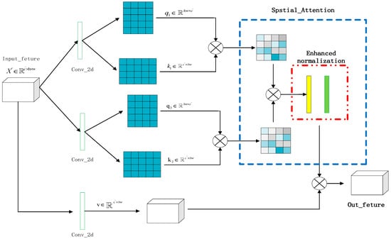
Figure 3. The SPA_ DAA module.

Here, $X^{\prime }$ is the input. ${\omega }_{q_1}$, ${\omega }_{q_2}$, ${\omega }_{k_1}$, ${\omega }_{k_2}$, and ${\omega }_v$ are the weight parameters of query $q_1$, $q_2$; key, $k_1$, $k_2$; and value, $v$, and these parameters are parameters that can be used for training. In addition, $F(•)$ in the formula is the 2D convolution kernel with size $1\times 1$.

After the query and the key point multiplication in the training process, some particularly large singular feature values will be obtained. This will cause the phenomenon of gradient explosion, resulting in poor training performance. However, the purpose of attention is only to make the value of the corresponding part of the features with high correlation larger, and the value of the corresponding part of the features with low correlation smaller. That is known as the importance difference of the obtained features. In traditional attention, softmax is usually used to normalize the attention maps, but this will make the gradient of some inputs become 0. This means that for the activation of this region, the weight will not be updated during the back propagation. Therefore, it will produce dead neurons that cannot be activated and ultimately affect the effect of classification. For this reason, the enhanced normalization strategy is proposed in the SPA_DAA. First, a global mean normalization is performed for all values, and then batch normalization is performed. Enhanced normalization not only solves the impact of singular feature values on network training, but also further enhances the ability of SPA_DAA to pay attention to spatial features. This is because the dot product of two groups of attention is used at the beginning, which is equivalent to the square of the feature values of a single attention. This makes the distance between the feature values and the non-interested feature values become larger. At this time, the mean normalization is equivalent to enhancing the features of interest and suppressing the features of non-interest. In this way, the SPA_DAA has further improved its attention ability through enhanced normalization support. The production process of attention maps can be represented as

$$att{n}_1=\left(q_1·k_1\right)q_1\in {ℝ}^{hw\times c^{\prime }},k_1\in {ℝ}^{c^{\prime }\times hw},att{n}_1\in {ℝ}^{hw\times hw}$$

(11)

$$att{n}_2=\left(q_2·k_2\right)q_2\in {ℝ}^{hw\times c^{\prime }},k_2\in {ℝ}^{c^{\prime }\times hw},att{n}_2\in {ℝ}^{hw\times hw}$$

(12)

$$attn=QIR\left(att{n}_1·att{n}_2;N\right)attn\in {ℝ}^{hw\times hw}$$

(13)

$$Attn=BN\left(attn\right)\in R^{hw\times hw}attn\in {ℝ}^{hw\times hw},Attn\in {ℝ}^{hw\times hw}$$

(14)

where $att{n}_1$ and $att{n}_2$ are obtained by the point multiplication of query tensor $q_1$ and value tensor $k_1$ and the point multiplication of query tensor $q_2$ and value tensor $k_2$, in turn. In Equation (13), after multiplying $att{n}_1$ and $att{n}_2$, divide all the resulting values by the mean $N$, and then round up to get $attn$, where $QIR(•)$ is a compound operation of division and rounding. In this way, the values can be uniformly weakened to prevent the generation of too-large singular values. $hw\times hw$ is the size of $att{n}_1$ and $att{n}_2$. In Equation (14), $Attn$ is the attention graph obtained, where Equations (13) and (14) can be simplified as

$$Attn=EB\left(att{n}_1·att{n}_2\right)$$

(15)

$EB(•)$ is a composite function of two operations of $QIR(•)$ and $BN(•)$. Because it is two consecutive normalization processes, it is called enhanced normalization. Finally, the output of the SPA_DAA module can be expressed as

$$Out\_F=v·Attn=v·EB\left(att{n}_1·att{n}_2\right)Out\_F\in {ℝ}^{c^{\prime }\times hw}$$

(16)

The value of each position of $Out\_F$ is reconstructed by multiplying the weighted value, $v$, with $Attn$. The detailed implementation process of SPA_DAA module is shown in Algorithm 2.

Algorithm 2. The detailed implementation process of SPA_DAA module

Input: the feature map $X^{\prime }\in {ℝ}^{c^{\prime }\times h\times w}$, where $X^{\prime }$ is the result of the nonlinear dimensionality reduction of feature $X$ obtained by the CDC module. Input X into three 2D convolutions to obtain $q_1\in {ℝ}^{hw\times c^{\prime }}$, $q_2\in {ℝ}^{hw\times c^{\prime }}$, and $v\in {ℝ}^{c^{\prime }\times hw}$, respectively. Then transpose $q_1$ and $q_2$ to obtain $k_1\in {ℝ}^{c^{\prime }\times hw}$ and $k_2\in {ℝ}^{c^{\prime }\times hw}$. Divide $q_1$ and $k_1$ into one group and $q_2$ and $k_2$ into another group. Multiply the two groups of query tensors and key tensors, respectively, to obtain $att{n}_1\in {ℝ}^{hw\times hw}$ and $att{n}_2\in {ℝ}^{hw\times hw}$. Then, multiply $att{n}_1$ and $att{n}_2$ to obtain the attention mask,$Attn$, through enhanced normalization processing. Output: finally, multiply the obtained attention mask with $v\in {ℝ}^{c^{\prime }\times hw}$ to obtain attention, $Out\_F\in {ℝ}^{c^{\prime }\times hw}$.

Similarly, a SPE_DAA is proposed on the spectral branch. As shown in Figure 4, unlike SPA_DAA, SPE_DAA uses 3D convolution kernels to build query, key, and value. While focusing on spectral characteristics, spatial locations are linked to establish correlations between spectral and spatial locations. Therefore, the SPE_DAA can not only focus on the feature differences of the constructed spectral information, but also associate the spatial spectral information. The calculation of query tensor, key tensor, and value tensor in the SPE_DAA can be expressed as

$$Q_1=G\left(X^{″};{\psi }_{Q_1}\right)X^{″}\in {ℝ}^{h\times w\times b,c^{\prime }},Q_1\in {ℝ}^{hw\times c^{\prime }}$$

(17)

$$Q_2=G\left(X^{″};{\psi }_{Q_2}\right)X^{″}\in {ℝ}^{h\times w\times b,c^{\prime }},Q_2\in {ℝ}^{hw\times c^{\prime }}$$

(18)

$$K_1=G\left(X^{″};{\psi }_{K_1}\right)X^{″}\in {ℝ}^{h\times w\times b,c^{\prime }},K_1\in {ℝ}^{c^{\prime }\times hw}$$

(19)

$$K_2=G\left(X^{″};{\psi }_{K_2}\right)X^{″}\in {ℝ}^{h\times w\times b,c^{\prime }},K_2\in {ℝ}^{c^{\prime }\times hw}$$

(20)

$$V=G\left(X^{″};{\psi }_V\right)X^{″}\in {ℝ}^{h\times w\times b,c^{\prime }},V\in {ℝ}^{c^{\prime }\times hw}$$

(21)

where, $Q_1$ and $Q_2$ are the queries of spectral branch. $K_1$ and $K_2$ are keys and $V$ is value. $G(•)$ is a 3D convolution operation. In fact, $Q_1$, $Q_2$, and $V$ in the SPE_DAA adopt the same settings, so the parameters are shared with each other. The calculation of the spectral attention map follows the idea of SPA_DAA and adopts the enhanced normalization strategy. The calculation process can be expressed as

$$attn\_ass{o}_1=\left(Q_1·K_1\right)attn\_ass{o}_1\in {ℝ}^{hw\times hw}$$

(22)

$$attn\_ass{o}_2=\left(Q_2·K_2\right)attn\_ass{o}_2\in {ℝ}^{hw\times hw}$$

(23)

$$Attn\_asso=EB\left(attn\_ass{o}_1·attn\_ass{o}_2\right)Attn\_asso\in {ℝ}^{hw\times hw}$$

(24)

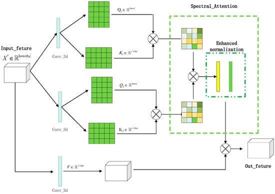
Figure 4. The SPE_ DAA module.

Among them, $attn\_ass{o}_1$ and $attn\_ass{o}_2$ are the spatial spectral-associated attention features obtained by the multiplication of query tensor and key tensor. In Equation (24), $Attn\_asso$ is the spectral attention map obtained by the enhanced normalization of two separate spatial spectral association attentions. Then, multiply $Attn\_asso$ with the value in Equation (21) to reconstruct the spatial spectral association information. This process can be expressed as

$$Out=V·Attn\_assoOut\in {ℝ}^{c^{\prime }\times hw}$$

(25)

It is worth noting that SPE_DAA does not only focus on the information of spectral dimension, but also closely associates the spectral with the spatial position, which makes the subsequent fusion of spatial and spectral branches more appropriate. The implementation process of SPE_DAA is shown in Algorithm 3.

Algorithm 3. The implementation process of the SPE_DAA module

Input: feature map $X^{″}\in {ℝ}^{h\times w\times b,c^{\prime }}$. $X^{″}$ is the feature obtained by the residual module. Reduce the spectral dimension of $X^{″}$ through the 3D convolution of size $1\times 1\times b$ and associate the spectral information with the spatial information. Then, it is processed by 3D convolutions and $Q_1\in {ℝ}^{hw\times c^{\prime }}$, $Q_2\in {ℝ}^{hw\times c^{\prime }}$, $V\in {ℝ}^{c^{\prime }\times hw}$, $K_1\in {ℝ}^{c^{\prime }\times hw}$, and $K_2\in {ℝ}^{c^{\prime }\times hw}$ are obtained, respectively. The $Q_1$ and the $K_1$ are divided into a group and the $Q_2$ and the $K_2$ are divided into a group. Multiply the two groups of query tensors and key tensors, respectively, to obtain $attn\_ass{o}_1\in {ℝ}^{hw\times hw}$ and $attn\_ass{o}_2\in {ℝ}^{hw\times hw}$. Then, multiply $attn\_ass{o}_1$ and $attn\_ass{o}_2$, and obtain the attention mask, $Attn\_asso$, through enhanced normalization processing. Output: multiply the obtained attention mask with $V\in {ℝ}^{c^{\prime }\times hw}$ to obtain attention, $Out\in {ℝ}^{c^{\prime }\times hw}$.

2.4. The Multi-Scale Head Strategy

Based on the DAA module, a multi-scale head mechanism is proposed. The multi-scale dual aggregated attention mechanism (MDAA) is composed of multi-scale head and the DAA, as shown in Figure 5. The upper part is composed of a multi-scale head mechanism and a SPA_DAA composition, namely, a spatial multi-scale dual aggregated attention (SPA_MDAA) module. The SPA_ MDAA uses two 2D convolutions of size $1\times 1$ and $3\times 3$ as its head. Different from the traditional multi-head mechanism of attention, multi-scale heads do not simply connect the attention of different heads but multiply the two to provide attention with greater attention ability. This way of processing restricts the number of channels to a certain extent. It also reduces the number of parameters and makes the calculation relatively simple. With the introduction of multi-scale convolution, the receptive field of attention has been well expanded.

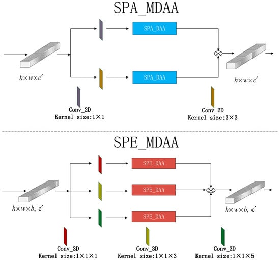
Figure 5. Multi-scale dual aggregated attention mechanism.

The multi-scale head mechanism is also designed on the SPE_DAA, as shown in the lower part of Figure 5. A spectral multi-scale dual aggregated attention (SPE_MDAA) module is composed of a multi-scale head mechanism and a SPE_DAA module. Three heads of different sizes are used in the SPE_MDAA. The three heads are three 3D convolutions with the sizes of $1\times 1\times 1$, $1\times 1\times 3$, and $1\times 1\times 5$. The SPA_ MDAA and the SPA_ MDAA are similar, and they are also the multiplication of a single attention.

3. Experimental Results and Analysis

First, four HSI data sets are introduced in detail. Then, the hyper-parameter setting of the experiment is described. In order to make a fair comparison, all experiments were conducted in the same environment. Specifically, the elected CPU is AMD Ryzen 75800H. The selected GPU is NVIDIA RTX 3070. The software environment for the experiment is CUDA11.2, Python 3.7.12, and torch 1.10.0.4 of Windows 10. Pycharm is used to compile software. In order to verify the effectiveness of the proposed module in the network, a large number of ablation experiments have been carried out in this paper. In addition, in order to obtain the best network performance, some comparative experiments were carried out and the best network structure was determined. Finally, in order to evaluate the performance of the method proposed in this paper, the network is quantitatively evaluated on four data sets using three important evaluation indicators: overall accuracy (OA), average accuracy (AA), and kappa coefficient. Their calculation process can be expressed as

$$OA=\frac{{\displaystyle {\sum }_{i=1}^n{s}_{i,i}}}{S}$$

(26)

$$AA=\frac{1}{n}{\displaystyle {\sum }_{i=1}^n\frac{s_{i,i}}{{\displaystyle {\sum }_{j=1}^n{s}_{i,j}}}}$$

(27)

$$Kappa=\frac{{\displaystyle \sum _{i=1}^n{s}_{i,j}-{\displaystyle \sum _{i=1}^n\left(s_{i,-}{\mathrm{s}}_{-,i}\right)}/S}}{S-{\displaystyle \sum _{i=1}^n\left(s_{i,-}{\mathrm{s}}_{-,i}\right)}/S}$$

(28)

where $S$ is the total number of samples and $s_{i,j}$ is the number of samples classified by category $i$ as category $j$; $n$ is the number of categories. In order to avoid the randomness of the experimental results, each group of experiments was repeated 10 times and then the averages of the 10 experimental results were taken as the final experimental results. In this paper, the best experimental results in the table are displayed in bold.

3.1. HSI Datasets

In order to verify the effectiveness of CDC_MDAA, the experiment described in this paper was conducted on four more challenging data sets, including Indian Pines (IN), Salinas Valley (SV), Kennedy Space Center (KSC), and Pavia University (UP), as shown in Figure 6. Figure 6a is a pseudo-color map of IN data set. The IN dataset uses the airborne visible infrared imaging spectrometer (AVIRIS) to continuously image ground objects in 220 continuous bands, and only 200 bands are reserved as the research object. There are 21,025 pixels in total, but only 1024 of them are ground object pixels, including 16 classes. The UP dataset is continuously imaged on 115 bands. In reality, only 103 spectral bands that are not polluted by noise are used for experiments. There are only 42,776 pixels of marked ground objects in the UP, a total of 9 types of ground objects. The pseudo-color map of UP is shown in Figure 6b. The pseudo-color map of the SV dataset is shown in Figure 6c. The SV contains 204 bands and 111,104 pixels. However, only 54,129 pixels can be used for classification, including 16 classes. The KSC contains 176 bands and 314,368 pixels. The marked ground objects have only 5211 pixels, including 13 classes. The pseudo-color map of KSC is shown in Figure 6d.

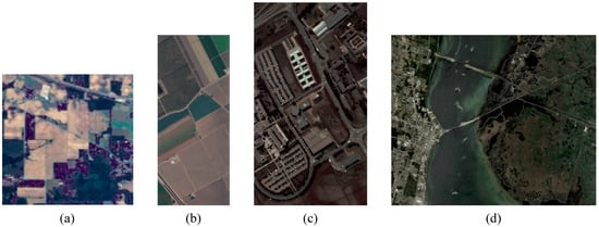
Figure 6. Pseudo-color maps of different data sets. (a) Pseudo-color map of IN; (b) pseudo-color map of SV; (c) pseudo-color map of UP; (d) pseudo-color map of KSC.

In this paper, the ground object classes and sample numbers of the four data sets are given, as shown in Table 1, Table 2, Table 3 and Table 4. In this paper, different sample proportions are used as training sets for different data sets. Among them, IN uses 3% of the samples as the training set, KSC uses 5% of the samples as the training set, and SV and UP use 0.5% of the samples as the training set.

Table 1. Ground object classes and sample numbers of IN.

Ground truth	NO.	Lengend	Name	Sample
	1		Alfafa	46
	2		Corn–n	1428
	3		Corn–m	830
	4		Corn	237
	5		Grass–p	483
	6		Grass–t	730
	7		Grass–p–m	28
	8		Hay-w	478
	9		Oats	20
	10		Soybean-n	972
	11		Soybean-m	2455
	12		Soybean-c	593
	13		Wheat	205
	14		Woods	1265
	15		Buildings-G-T	386
	16		Stone-S-T	93

Table 2. Ground object classes and sample numbers of UP.

Ground truth	NO.	Lengend	Name	Sample
	1		Asphalt	6631
	2		Meadows	18,649
	3		Gravel	2099
	4		Trees	3064
	5		Painted m s	1345
	6		B Soil	5029
	7		Bitumen	1330
	8		S-B Bricks	3682
	9		Shadows	947

Table 3. Ground object classes and sample numbers of SV.

Ground truth	NO.	Lengend	Name	Sample
	1		weeds_1	2009
	2		weeds_2	3726
	3		Fallow	1976
	4		Fallow-r-p	1394
	5		Fallow-s	2678
	6		Stubble	3959
	7		Celery	3579
	8		Grapes-u	11,271
	9		Soil-v-y-d	6203
	10		C-s-g-weeds	3278
	11		L-r-4wk	1068
	12		L-r-5wk	1927
	13		L-r-6wk	916
	14		L-r-7wk	1070
	15		VIN-yard-u	7268
	16		VIN-yard-v-t	1807

Table 4. Ground object classes and sample numbers of KSC.

Ground truth	NO.	Lengend	Name	Sample
	1		Scrub	761
	2		W swamp	243
	3		CP hammock	256
	4		Slash pine	252
	5		Oak/Broadleaf	161
	6		Hardwood	229
	7		Grass-p-m	105
	8		G marsh	431
	9		Sp marsh	520
	10		C marsh	404
	11		Sa marsh	419
	12		Mud flats	503
	13		Water	927

3.2. Experimental Parameters and Model Setting

In this part, the experimental parameters are set, and the best model is determined.

3.2.1. Experimental Parameter Setting

The epoch of the network is set to 400 and the batch size is set to 64. Because the learning rate strategy of cosine annealing is adopted, a small learning rate can avoid the problem of local optimal solution. But a too-small learning rate will make the model difficult to converge. In addition, the input size of the patch will also affect the performance of the network. In order to find the best hyper-parameter for the network, this paper explores the influence of input patch size on the accuracy under different learning rates. As shown in Figure 7, the experimental results are drawn into surface maps. On the four data sets, the surface maps show a convex shape, and the convex part is concentrated around a $9\times 9$ patch and 0.001 learning rate. This shows that when the patch size is $9\times 9$ and the learning rate is 0.001, the classification performance of the network is the best. Therefore, the patch size is set to $9\times 9$ and the learning rate is set to 0.001 in CDC_MDAA.

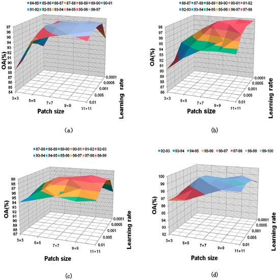
Figure 7. Effect of input patch size on accuracy at different learning rate. (a) IN, (b) SV, (c) UP, (d) KSC.

3.2.2. Model Setting

In the overall framework of the model, two SPA_MDAA modules are selected as spatial attention modules and two SPE_MDAA modules are selected as spectral attention modules. In order to verify the advantages of this structure in CDC_MDAA, several groups of experiments were carried out on the more challenging IN. The experimental results are shown in Figure 8, where $1SPE\_MDAA+1SPA\_MDAA$ represents the combination of one SPE_MDAA module and one SPA_MDAA module. By analogy, the experiment was set to 9 groups. By comparing the experimental results obtained under the combination of $2SPE\_MDAA+2SPA\_MDAA$, the network obtained the maximum OA value of 96.94%, the maximum KAPPA value of 96.51%, and the larger AA value of 94.31%. The results show that when two SPE_MDAA modules are selected as spectral attention modules and two SPA_MDAA modules are selected as spatial attention modules, the network can show the best classification performance.

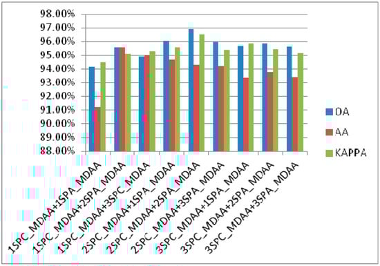
Figure 8. Classification accuracy of different combinations of the SPA_MDAA and the SPE_MDAA in IN.

In this part, the number of multi-scale heads is also compared. The experimental results are shown in Figure 9.

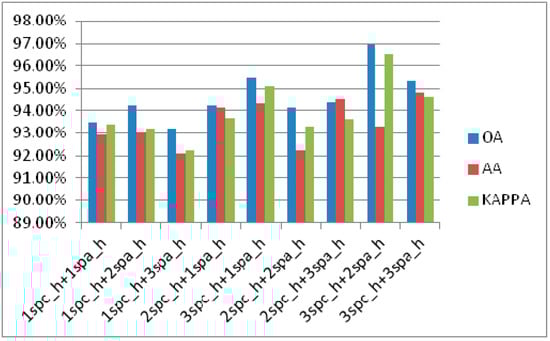
Figure 9. Classification accuracy of CDC_MDAA with different number of headers on IN dataset.

In Figure 9, spc_h represents the spectral attention head, and spa_h represents the spatial attention head. It can be seen from the experimental results that OA and KAPPA can obtain the best performance when $3spa\_h+2spe\_h$ is selected. Therefore, the $3spa\_h+2spe\_h$ structure is selected in the CDC_MDAA network.

3.3. Experimental Analysis

3.3.1. Effectiveness Analysis of the Proposed Module

In this part, a large number of ablation experiments have been performed to verify the effectiveness of the proposed CDC, SPA_MDAA and SPE_MDAA. The experimental results are shown in Table 5, Table 6 and Table 7. The effectiveness of CDC is analyzed in Table 5. It can be seen from Table 5 that, compared with the strategy without CDC, OA, AA, KAPPA of the strategy with CDC has increased by 4.23%, 0.29%, and 4.77%, respectively. Obviously, CDC can greatly improve the classification performance of the network. This is because CDC can realize cross-channel information interaction, and repeatedly use feature information through dense connection, which more effectively extract spatial features. The classification results of the ablation experiment on SPA_MDAA are shown in Table 6. It can be seen that, the classification performance of the network has been significantly improved after integrating SPA_MDAA into CDC_MDAA. Compared with the CDC_MDAA without SPA_MDAA, OA increases by 8.18%, AA increases by 9.07%, and KAPPA increases by 10.68%, which is fully prove the effectiveness of the proposed SPA_MDAA. Finally, the effectiveness of SPE_MDAA is analyzed in this paper, as shown in Table 7. Compared with CDC_MDAA without SPE_MDAA, the OA, AA, and KAPPA of CDC_MDAA with SPE_MDAA has increased by 5.49%, 2% and 3.96%, respectively. Therefore, SPE_MDAA has also greatly improved the classification performance of CDC_MDAA.

Table 5. Effectiveness analysis of CDC.

STRATEGY	OA	AA	KAPPA
Without CDC	92.71%	94.02%	91.74%
With CDC	96.94%	94.31%	96.51%

Table 6. Effectiveness analysis of SPA_MDAA.

STRATEGY	OA	AA	KAPPA
Without SPA_MDAA	88.76%	85.24%	85.83%
With SPA_MDAA	96.94%	94.31%	96.51%

Table 7. Effectiveness analysis of SPE_MDAA.

STRATEGY	OA	AA	KAPPA
Without SPE_MDAA	91.45%	92.31%	92.55%
With SPE_MDAA	96.94%	94.31%	96.51%

3.3.2. Convergence of Network

In order to verify the convergence of CDC_MDAA, the variation in the loss value during the process of training with the number of iterations and the variation in the accuracy with the number of iterations are provided, which are shown in Figure 10. On four different data sets, the training accuracy and verification accuracy of CDC_MDAA show an upward trend with the increase in the number of training iterations. The corresponding training loss and verification loss showed a downward trend. In addition, the training accuracy is very close to the verification accuracy, which has good fitting. It is worth noting that while the training loss value and the verification loss value continue to decline with the training, there is no significant fluctuation. The overall downward trend is smooth, which also shows that the network has good stability in convergence.

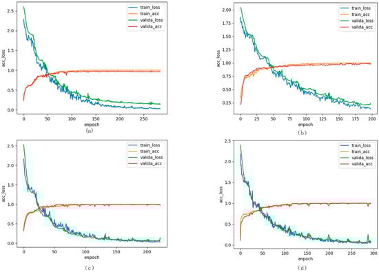
Figure 10. (a) training loss, training accuracy, verification loss, and verification accuracy on IN dataset, (b) training loss, training accuracy, verification loss, and verification accuracy on UP dataset, (c) training loss, training accuracy, verification loss, and verification accuracy on SV dataset, (d) training loss, training accuracy, verification loss, and verification accuracy on KSC dataset.

3.3.3. Comparison of Different Methods

To further verify the effectiveness and generalization of the proposed CDC_MDAA, this paper compares CDC_MDAA with some mainstream classification methods, including SVM [47], CDCNN [48], FDSSC [49], SSRN [50], DBMA, DBDA, DTAN [51], and FECNet [52]. The classification results of all methods on different data sets are shown in Table 8, Table 9, Table 10 and Table 11. First, from the perspective of evaluation indicators (OA, AA, KAPPA), compared with other methods, the classification accuracy of CDC_MDAA is always obviously higher than that of other methods. This demonstrates that CDC_MDAA can provide superior classification performance. In addition, from the perspective of network generalization, the proposed method can show stable classification performance on all four data sets. However, the classification performance of other networks on different data sets is uneven. For example, the classification performance of the DTAN network is good on the SV data set in Table 10 but its classification performance on the other three data sets is somewhat unsatisfactory. The proposed CDC_MDAA can always achieve the highest OA, AA, and KAPPA on four different data sets. This proves that CDC_MDAA has excellent generalization ability and can adapt to datasets in different scenarios. Finally, the training and testing times for different methods are also presented in Table 8, Table 9, Table 10 and Table 11. It can be seen that CDCNN has the shortest training and testing time on different datasets. This is because the structure of CDCNN is very simple and the network layer is shallow, which makes the classification accuracy of CDCNN very poor. However, the proposed method needs less runtime compared to the vast majority of methods while ensuring classification performance. This demonstrates the advantages of the proposed method in terms of network complexity.

Table 8. Classification results of different methods on IN dataset.

Class	SVM	SSRN	FDSSC	CDCNN	DBMA	DBDA	DTAN	FECNet	Proposed
1	36.62	81.03	85.72	24.67	77.33	99.06	30.00	99.06	100.0
2	55.48	87.48	93.35	49.93	78.68	92.74	93.87	96.63	98.84
3	62.33	76.35	89.51	31.93	76.12	92.28	95.12	93.25	98.69
4	42.53	73.88	93.68	33.52	75.11	94.46	94.55	95.61	95.41
5	85.05	84.28	92.61	71.47	94.91	99.10	94.63	98.55	100.0
6	83.31	92.68	98.31	73.42	93.99	98.28	99.21	97.51	96.89
7	59.86	79.06	82.46	36.29	44.33	66.57	50.00	73.14	62.50
8	89.67	96.85	97.54	78.08	97.49	99.24	92.73	99.84	100.0
9	39.27	73.57	71.07	42.14	45.66	93.64	20.00	79.71	84.21
10	62.31	84.45	89.30	41.71	77.27	93.77	92.50	90.09	89.49
11	64.72	86.95	93.97	55.67	83.89	93.83	93.55	96.11	98.97
12	50.54	83.31	88.25	27.68	77.65	90.65	89.12	93.20	95.85
13	86.73	98.83	99.53	67.88	96.74	97.48	99.89	98.34	100.0
14	88.67	95.13	95.82	76.39	93.41	97.69	95.31	97.28	95.87
15	61.81	88.58	92.48	47.30	76.83	93.79	93.54	95.11	96.75
16	98.66	96.52	98.22	65.67	92.33	93.67	93.21	97.26	95.45
OA(%)	68.76	86.68	92.37	59.19	82.38	92.26	93.47	95.47	96.94
AA(%)	66.72	86.18	91.36	51.48	80.11	92.90	81.66	93.79	94.31
$KAPPA\times 100$	63.98	84.76	91.30	0.781	79.86	91.24	92.48	94.83	96.51
Trian time	——	619.8 s	1414.0 s	35.6 s	279.5 s	280.1 s	112.5 s	340.2 s	143.3 s
Test time	——	4.68 s	9.88 s	1.8 s	16.3 s	16.4 s	10.2 s	15.9 s	9.3 s

Table 9. Classification results of different methods on UP dataset.

Class	SVM	SSRN	FDSSC	CDCNN	DBMA	DBDA	DTAN	FECNet	Proposed
1	81.26	93.22	84.30	79.88	89.41	90.77	63.87	96.77	97.91
2	84.52	93.75	95.47	86.66	94.34	98.07	95.59	99.20	99.40
3	56.56	64.97	80.58	32.74	84.99	90.04	83.68	96.56	98.77
4	94.34	94.69	98.13	84.88	96.58	97.96	97.03	97.87	98.17
5	95.38	97.69	99.21	94.77	98.06	98.67	96.43	97.38	99.92
6	80.66	93.14	92.36	71.54	94.60	98.85	98.10	97.72	98.30
7	49.13	73.06	69.35	31.77	93.18	96.95	19.18	96.50	100.0
8	73.15	79.98	73.36	65.54	76.61	87.65	81.82	87.34	95.29
9	97.93	98.71	97.39	73.40	91.45	97.81	50.00	98.98	99.46
OA	82.06	89.12	90.71	80.69	90.98	95.32	86.36	96.96	98.59
AA	79.21	87.69	87.91	69.02	91.02	95.20	76.19	96.48	98.58
$KAPPA\times 100$	75.43	85.44	87.38	73.45	87.87	93.77	81.52	95.97	98.13
Trian time	——	401.5 s	933.8 s	26.0 s	82.4 s	83.0 s	54.9 s	140.8 s	76.9 s
Test time	——	12.3 s	25.2 s	7.4 s	39.4 s	39.8 s	45.6 s	41.1 s	6.9 s

Table 10. Classification results of different methods on SV dataset.

Class	SVM	SSRN	FDSSC	CDCNN	DBMA	DBDA	DTAN	FECNet	Proposed
1	99.42	99.53	99.96	68.15	99.98	99.68	99.45	100.0	100.0
2	98.79	99.53	98.90	73.63	99.20	98.88	99.61	99.95	99.57
3	87.98	94.22	96.91	75.56	97.65	97.94	99.39	98.41	95.18
4	97.54	96.98	94.54	92.79	92.64	94.89	92.65	95.85	95.17
5	95.09	98.84	99.16	92.90	98.79	98.40	99.81	99.64	99.77
6	99.89	99.87	99.82	96.25	98.49	99.92	99.53	99.89	100.0
7	95.59	98.21	98.16	93.76	98.41	98.46	93.10	99.40	100.0
8	71.66	86.20	91.72	74.03	90.72	90.87	89.98	94.79	95.75
9	98.08	99.14	99.53	94.72	99.61	99.24	99.62	99.67	99.48
10	85.39	97.99	97.61	76.65	92.23	97.62	99.29	98.01	97.45
11	86.97	94.48	95.70	69.32	93.10	94.92	94.90	97.18	95.15
12	94.20	98.53	98.16	80.43	99.24	99.54	99.59	99.55	100.0
13	93.43	98.28	98.35	69.55	98.56	99.76	99.52	99.94	100.0
14	92.03	96.05	96.21	87.22	96.56	96.66	88.16	96.51	97.15
15	71.02	81.04	89.07	63.71	88.27	90.48	92.25	93.68	96.13
16	97.81	99.48	99.77	98.38	99.68	99.83	99.98	100.0	100.0
OA(%)	86.97	92.51	95.91	80.67	94.77	95.74	96.25	97.49	97.88
AA(%)	91.55	96.32	97.49	81.69	96.45	97.41	97.36	98.01	98.17
$KAPPA\times 100$	85.45	91.67	95.45	78.35	94.18	95.26	95.86	97.21	97.63
Trian time	——	531.9 s	1212.3 s	59.7 s	246.1 s	247.2 s	130.7 s	310.5 s	182.0 s
Test time	——	27.4 s	56.1 s	9.5 s	91.7	92.1 s	58.6 s	96.9 s	9.6 s

Table 11. Classification results of different methods on KSC dataset.

Class	SVM	SSRN	FDSSC	CDCNN	DBMA	DBDA	DTAN	FECNet	Proposed
1	92.42	98.67	99.56	94.53	99.96	99.91	50.70	99.97	100.0
2	87.14	93.49	94.69	72.91	92.06	96.97	43.07	98.28	99.09
3	72.46	91.10	85.99	53.64	87.01	93.40	14.46	94.06	100.0
4	54.45	81.73	82.92	42.40	76.56	83.97	69.25	88.95	90.65
5	64.10	77.45	74.32	25.00	70.60	79.76	0.000	94.26	97.77
6	65.23	95.85	96.67	64.45	93.22	97.65	13.25	97.94	100.0
7	75.49	91.96	96.48	49.77	82.73	92.73	20.00	97.94	93.62
8	87.33	98.24	99.39	71.63	95.31	99.57	73.33	99.9	99.74
9	87.94	98.11	99.91	80.68	96.76	99.91	55.29	98.11	100.0
10	97.01	99.81	100.0	81.92	98.40	99.89	87.17	100.0	100.0
11	96.02	99.06	99.07	98.49	99.01	99.46	100.0	98.93	100.0
12	93.76	99.76	99.73	92.56	99.01	99.41	89.80	99.62	99.34
13	99.72	100.0	100.0	99.10	100.0	100.0	99.07	100.0	100.0
OA(%)	87.95	96.35	96.42	81.24	95.07	97.55	70.32	98.14	99.19
AA(%)	82.54	94.26	94.52	71.31	92.68	95.59	55.03	97.53	98.48
$KAPPA\times 100$	86.59	95.93	96.01	79.08	94.51	97.27	66.24	97.93	99.10
Trian time	——	504.7 s	1159.6 s	30.49 s	196.5 s	198.5 s	86.4 s	259.7 s	166.9 s
Test time	——	2.05 s	4.34 s	0.88 s	7.2 s	7.2 s	5.0 s	7.3 s	3.6 s

The classification maps obtained by all networks are shown in Figure 11, Figure 12, Figure 13 and Figure 14. It can be seen that all methods can effectively classify hyperspectral images. However, compared with CDC_MDAA, the classification maps of other methods have more noise and more false classification. This is due to the relatively weak feature extraction ability of other methods and the inability to highlight important features. It is worth noting that CDC_MDAA can provide clearer boundaries than other networks on the four data sets and can distinguish different types of ground objects more clearly, which is closer to the ground truth. It benefits from the excellent feature extraction ability of the CDC module. Moreover, the difference processing of features by dual aggregated attention can highlight important features and enhance the discriminating ability of the network. Therefore, it has better classification performance of hyperspectral images.

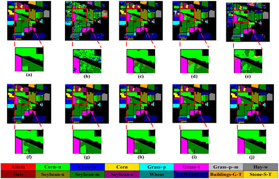
Figure 11. Classification maps on IN dataset, (a) ground truth, (b) SVM, (c) SSRN, (d) FDSSC, (e) CDCNN, (f) DBMA, (g) DBDA, (h) DTAN, (i) FECNet, (j) proposed.

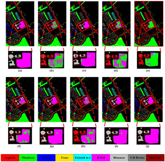
Figure 12. Classification maps on UP dataset, (a) ground truth, (b) SVM, (c) SSRN, (d) FDSSC, (e) CDCNN, (f) DBMA, (g) DBDA, (h) DTAN, (i) FECNet, (j) proposed.

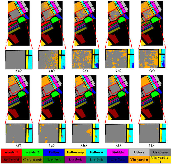
Figure 13. Classification maps on SV dataset, (a) ground truth, (b) SVM, (c) SSRN, (d) FDSSC, (e) CDCNN, (f) DBMA, (g) DBDA, (h) DTAN, (i) FECNet, (j) proposed.

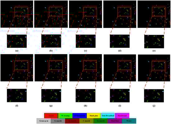
Figure 14. Classification maps on KSC dataset, (a) ground truth, (b) SVM, (c) SSRN, (d) FDSSC, (e) CDCNN, (f) DBMA, (g) DBDA, (h) DTAN, (i) FECNet, (j) proposed.

The classification results of all methods with different training sample numbers on four data sets are shown in Figure 15. It can be seen from Figure 15a that no matter how many training samples are used in the IN, the CDC_MDAA network is superior to other networks. The advantages of CDC_MDAA are more prominent in the case of smaller training samples. For example, when the training sample is only 1% of the total sample, CDC_ MDAA can show far higher classification accuracy than other methods. For SV and UP with a large number of samples, CDC_ MDAA can also maintain its advantages. It is worth noting that on the KSC with a total sample size of only 5211, CDC_ MDAA can still achieve the best classification results. It is proved that the proposed method is more conducive to the classification of hyperspectral images with small samples. In addition, it can be seen from Figure 15 that the classification performance of other networks fluctuates greatly under different training sample numbers. However, the CDC_MDAA can show stable classification performance in all cases. This further proves the powerful generalization of CDC_ MDAA. For the classification of hyperspectral images, the CDC_ MDAA can provide superior classification performance, surpassing other current mainstream methods when the number of training samples is small.

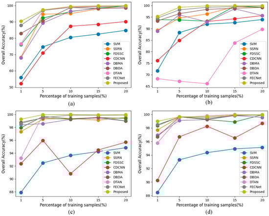
Figure 15. Classification results of all methods with different number of training samples on four data sets. (a) IN, (b) KSC dataset, (c) SV, (d) UP.

In order to verify the feature extraction performance of the proposed method, this paper uses t-distributed stochastic neighbor embedding (T-SNE) [53] to visually analyze the feature maps extracted by different methods. As shown in Figure 16 and Figure 17, four more competitive methods (including DBDA, FECNet, FDSSC, and DTAN) are chosen to compare with CDC_MDAA on SV and UP. In general, for SV and UP, all methods can realize feature clustering. However, HSIC is a multi-classification problem, and simple clustering is unable to meet the requirements of high-performance classification. It can be seen from Figure 16 that the other four methods cannot clearly divide the adjacent classes on SV, shown by “Grapes-u” and “VIN-yard-v-t”. Compared with the other four methods, the method proposed in this paper can better distinguish the two classes. It proves CDC_ MDAA has excellent feature extraction capability. In addition, CDC_ MDAA enhances the separability of features by DAA, making it easier for the network to extract important features more conducive to classification and avoiding the interference of adjacent classes. The same conclusion can be reached on the UP dataset.

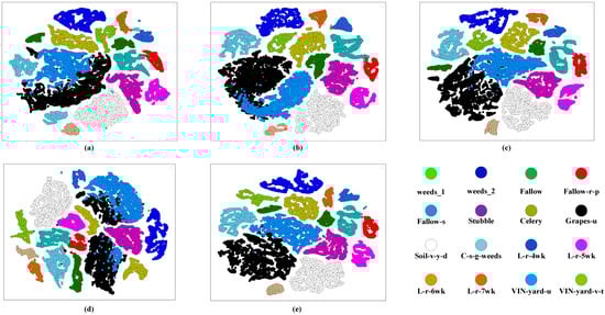
Figure 16. Visualization of feature separability for different methods on SV. (a) DBDA, (b) FECNet, (c) FDSSC, (d) DTAN, (e) Proposed.

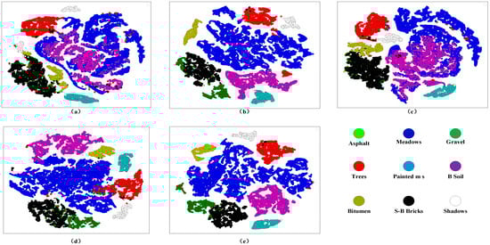
Figure 17. Visualization of feature separability for different methods on UP. (a) DBDA, (b) FECNet, (c) FDSSC, (d) DTAN, (e) Proposed.

4. Conclusions

In this paper, a novel CDC_MDAA network is proposed, which can effectively classify hyperspectral images. The CDC_ MDAA first extracts spectral and spatial features through double branches, then spectral attention and spatial attention mechanisms are utilized to focus on the extracted spatial and spectral features, respectively. Then, a spatial spectral attention fusion method is followed. Specifically, on the spatial branch, a CDC method is proposed to extract spatial features, and a SPA_MDAA module is designed to focus on spatial features. On the spectral branch, after feature extraction, a SPE_MDAA module is constructed to focus on spectral features. Finally, the double branches are fused and classified. CDC_ MDAA can achieve high classification accuracy in the case of small samples. This provides a new idea to solve the small sample problem of hyperspectral image classification. A large number of experimental results show that CDC_ MDAA can provide classification performance that is superior to some state-of-the-art methods, and it has good generalization.

References

- Bioucas-Dias, J.M.; Plaza, A.; Camps-Valls, G.; Scheunders, P.; Nasrabadi, N.; Chanussot, J. Hyperspectral remote sensing data analysis and future challenges. IEEE Geosci. Remote Sens. Mag. 2013, 1, 6–36. [Google Scholar] [CrossRef]
- Landgrebe, D. Hyperspectral image data analysis. IEEE Signal Process. Mag. 2002, 19, 17–28. [Google Scholar] [CrossRef]
- Lacar, F.M.; Lewis, M.M.; Grierson, I.T. “Use of hyperspectral imagery for mapping grape varieties in the Barossa Valley, South Australia”, IGARSS 2001. Scanning the Present and Resolving the Future. In Proceedings of the IEEE 2001 International Geoscience and Remote Sensing Symposium (Cat. No.01CH37217), Sydney, NSW, Australia, 9–13 July 2001; Volume 6, pp. 2875–2877. [Google Scholar]
- Stuffler, T.; Förster, K.; Hofer, S.; Leipold, M.; Sang, B.; Kaufmann, H.; Penné, B.; Mueller, A.; Chlebek, C. Hyperspectral imaging an advanced instrument concept for the Enmap mission (environmental mapping and analysis programme). Acta Astronaut. 2009, 65, 1107–1112. [Google Scholar] [CrossRef]
- Malthus, T.J.; Mumby, P.J. Remote sensing of the coastal zone: An overview and priorities for future research. Int. J. Remote Sens. 2003, 24, 2805–2815. [Google Scholar] [CrossRef]
- Fauvel, M.; Tarabalka, Y.; Benediktsson, J.A.; Chanussot, J.; Tilton, J.C. Advances in spectral-spatial classification of hyperspectral images. Proc. IEEE 2013, 101, 652–675. [Google Scholar] [CrossRef]
- Samaniego, L.; Bardossy, A.; Schulz, K. Supervised classification of remotely sensed imagery using a modified k-NN technique. IEEE Trans. Geosci. Remote Sens. 2008, 46, 2112–2125. [Google Scholar] [CrossRef]
- Ediriwickrema, J.; Khorram, S. Hierarchical maximum-likelihood classification for improved accuracies. IEEE Trans. Geosci. Remote Sens. 1997, 35, 810–816. [Google Scholar] [CrossRef]
- Foody, G.M.; Mathur, A. A relative evaluation of multi-class image classification by support vector machines. IEEE Trans. Geosci. Remote Sens. 2004, 42, 1335–1343. [Google Scholar] [CrossRef]
- Prasad, S.; Bruce, L.M. Limitations of princinal components analysis for hyperspectral target recognition. IEEE Geosci. Remote Sens. Lett. 2008, 5, 625–629. [Google Scholar] [CrossRef]
- Benediktsson, J.A.; Chanussot, J.; Moon, W.M. Very high-resolution remote sensing: Challenges and opportunities [point of view]. Proc. IEEE 2012, 100, 1907–1910. [Google Scholar] [CrossRef]
- Chen, Y.S.; Zhao, X.; Jia, X.P. Spectral-spatial classification of hyperspectral data based on deep belief network. IEEE J. Sel. Top. Appl. Earth Obs. Remote Sens. 2015, 8, 2381–2392. [Google Scholar] [CrossRef]
- Sun, L.; Wu, Z.B.; Liu, J.J.; Xiao, L.; Wei, Z.H. Supervised spectral-spatial hyperspectral image classification with weighted Markov random fields. IEEE Trans. Geosci. Remote Sens. 2015, 53, 1490–1503. [Google Scholar] [CrossRef]
- Chen, Y.S.; Lin, Z.H.; Zhao, X.; Wang, G.; Gu, Y.F. Deep learning based classification of hyperspectral data. IEEE J. Sel. Top. IN Appl. Earth Obs. Remote Sens. 2014, 7, 2094–2107. [Google Scholar] [CrossRef]
- Yuan, Y.; Meng, X.; Sun, W.; Yang, G.; Wang, L.; Peng, J.; Wang, Y. Multi-Resolution Collaborative Fusion of SAR, Multispectral and Hyperspectral Images for Coastal Wetlands Mapping. Remote Sens. 2022, 14, 3492. [Google Scholar] [CrossRef]
- Sun, W.; Kai Liu Ren, G.; Liu, W.; Yang, G.; Meng, X.; Peng, J. A simple and effective spectral-spatial method for mapping large-scale coastal wetlands using China ZY1-02D satellite hyperspectral images. Int. J. Appl. Earth Obs. Geoinf. 2021, 104, 102572. [Google Scholar] [CrossRef]
- Yang, J.; Zhang, D.; Frangi, A.F.; Yang, J.Y. Two-dimensional PCA: A new approach to appearance-based face representation and recognition. IEEE Trans. Pattern Anal. Mach. Intell. 2004, 26, 131–137. [Google Scholar] [CrossRef]
- Li, W.; Wu, G.; Zhang, F.; Du, Q. Hyperspectral image classification using deep pixel-pair features. IEEE Trans. Geosci. Remote Sens. 2017, 55, 844–853. [Google Scholar] [CrossRef]
- Makantasis, K.; Karantzalos, K.; Doulamis, A.; Doulamis, N. Deep supervised learning for hyperspectral data classification through convolutional neural networks. In Proceedings of the 2015 IEEE International Geoscience and Remote Sensing Symposium (IGARSS), Milan, Italy, 26–31 July 2015; pp. 4959–4962. [Google Scholar]
- Shao, W.; Du, S. Spectral-spatial feature extraction for hyperspectral image classification: A dimension reduction and deep learning approach. IEEE Trans. Geosci. Remote Sens. 2016, 54, 4544–4554. [Google Scholar]
- Mei, S.; Ji, J.; Hou, J.; Li, X.; Du, Q. Learning sensor-specific spatial-spectral features of hyperspectral images via convolutional neural networks. IEEE Trans. Geosci. Remote Sens. 2017, 55, 4520–4533. [Google Scholar] [CrossRef]
- Yue, J.; Zhao, W.; Mao, S.; Liu, H. Spectral-spatial classification of hyperspectral images using deep convolutional neural networks. Remote Sens. Lett. 2015, 6, 468–477. [Google Scholar] [CrossRef]
- Lecun, Y.; Bengio, Y.; Hinton, G. Deep learning. Nature 2015, 521, 436. [Google Scholar] [CrossRef]
- Ghamisi, P.; Maggiori, E.; Li, S.; Souza, R.; Tarablaka, Y.; Moser, G.; De Giorgi, A.; Fang, L.; Chen, Y.; Chi, M.; et al. New frontiers IN spectral-spatial hyperspectral image classification: The latest advances based on mathematical morphology, Markov random fields, segmentation, sparse representation, and deep learning. IEEE Geosci. Remote Sens. Mag. 2018, 6, 10–43. [Google Scholar] [CrossRef]
- Chen, Y.; Jiang, H.; Li, C.; Jia, X.; Ghamisi, P. Deep feature extraction and classification of hyperspectral images based on convolutional neural networks. IEEE Trans. Geosci. Remote Sens. 2016, 54, 6232–6251. [Google Scholar] [CrossRef]
- He, K.; Zhang, X.; Ren, S.; Sun, J. Deep residual learning for image recognition. In Proceedings of the IEEE Conference on Computer Vision and Pattern Recognition, Las Vegas, NV, USA, 27–30 June 2016; pp. 770–778. [Google Scholar]
- Paoletti, M.E.; Haut, J.M.; Plaza, J.; Plaza, A. Deep&dense convolutional neural network for hyperspectral image classification. Remote Sens. 2018, 10, 1454. [Google Scholar]
- Yu, C.; Han, R.; Song, M.; Liu, C.; Chang, C.-I. Feedback Attention-Based Dense CNN for Hyperspectral Image Classification. IEEE Trans. Geosci. Remote Sens. 2022, 60, 5501916. [Google Scholar] [CrossRef]
- Zhao, C.; Qin, B.; Li, T.; Feng, S.; Yan, Y. Hyperspectral Image Classification Based on Dense Convolution and Conditional Random Field. In Proceedings of the 2021 IEEE International Geoscience and Remote Sensing Symposium IGARSS, Brussels, Belgium, 11–16 July 2021; pp. 3653–3656. [Google Scholar]
- Zhang, H.; Yu, H.; Xu, Z.; Zheng, K.; Gao, L. A Novel Classification Framework for Hyperspectral Image Classification Based on Multi-Scale Dense Network. In Proceedings of the 2021 IEEE International Geoscience and Remote Sensing Symposium IGARSS, Brussels, Belgium, 11–16 July 2021; pp. 2238–2241. [Google Scholar]
- Yang, G.; Gewali, U.B.; Ientilucci, E.; Gartley, M.; Monteiro, S.T. Dual-Channel Densenet for Hyperspectral Image Classification. In Proceedings of the IGARSS 2018—2018 IEEE International Geoscience and Remote Sensing Symposium, Valencia, Spain, 22–27 July 2018; pp. 2595–2598. [Google Scholar]
- Paoletti, M.E.; Haut, J.M.; Fernandez-Beltran, R.; Plaza, J.; Plaza, A.J.; Pla, F. Deep Pyramidal Residual Networks for Spectral–Spatial Hyperspectral Image Classification. IEEE Trans. Geosci. Remote Sens. 2019, 57, 740–754. [Google Scholar] [CrossRef]
- Pande, S.; Banerjee, B. Dimensionality Reduction Using 3D Residual Autoencoder for Hyperspectral Image Classification. In Proceedings of the IGARSS 2020—2020 IEEE International Geoscience and Remote Sensing Symposium, Waikoloa, HI, USA, 19–24 July 2020; pp. 2029–2032. [Google Scholar]
- Zhang, C.; Li, G.; Du, S. Multi-Scale Dense Networks for Hyperspectral Remote Sensing Image Classification. IEEE Trans. Geosci. Remote Sens. 2019, 57, 9201–9222. [Google Scholar] [CrossRef]
- Li, Z.; Wang, T.; Li, W.; Du, Q.; Wang, C.; Liu, C.; Shi, X. Deep Multilayer Fusion Dense Network for Hyperspectral Image Classification. IEEE J. Sel. Top. Appl. Earth Obs. Remote Sens. 2020, 13, 1258–1270. [Google Scholar] [CrossRef]
- Wang, X.; Tan, K.; Du, P.; Pan, C.; Ding, J. A Unified Multiscale Learning Framework for Hyperspectral Image Classification. IEEE Trans. Geosci. Remote Sens. 2022, 60, 4508319. [Google Scholar] [CrossRef]
- Haut, Z.M.; Paoletti, M.E.; Plaza, J.; Plaza, A.; Li, J. Visual attention-driven hyperspectral image classification. IEEE Trans. Geosci. Remote Sens. 2019, 57, 8065–8080. [Google Scholar] [CrossRef]
- Woo, S.; Park, J.; Lee, J.; Kweon, I. Cbam: Convolutional block attention module. In Proceedings of the European Conference on Computer Vision (ECCV), Amsterdam, The Netherlands, 8–16 October 2018; pp. 3–19. [Google Scholar]
- Sun, H.; Zheng, X.; Lu, X.; Wu, S. Spectral–spatial attention network for hyperspectral image classification. IEEE Trans. Geosci. Remote Sens. 2020, 58, 3232–3245. [Google Scholar] [CrossRef]
- Mei, X.; Pan, E.; Ma, Y.; Dai, X.; Huang, J.; Fan, F.; Du, Q.; Zheng, H.; Ma, J. Spectral–spatial attention networks for hyperspectral image classification. Remote Sens. 2019, 11, 963. [Google Scholar] [CrossRef]
- Hang, R.; Li, Z.; Liu, Q.; Ghamisi, P.; Bhattacharyya, S.S. Hyperspectral Image Classification with Attention-Aided CNNs. IEEE Trans. Geosci. Remote Sens. 2021, 59, 2281–2293. [Google Scholar] [CrossRef]
- Zheng, X.; Sun, H.; Lu, X.; Xie, W. Rotation-Invariant Attention Network for Hyperspectral Image Classification. IEEE Trans. Image Process. 2022, 31, 4251–4265. [Google Scholar] [CrossRef] [PubMed]
- Yang, K.; Sun, H.; Zou, C.; Lu, X. Cross-Attention Spectral–Spatial Network for Hyperspectral Image Classification. IEEE Trans. Geosci. Remote Sens. 2022, 60, 5518714. [Google Scholar] [CrossRef]
- Ma, W.; Yang, Q.; Wu, Y.; Zhao, W.; Zhang, X. Double-Branch Multi-Attention Mechanism Network for Hyperspectral Image Classification. Remote Sens. 2019, 11, 1307. [Google Scholar] [CrossRef]
- Fu, J.; Liu, J.; Tian, H.; Li, Y.; Bao, Y.; Fang, Z.; Lu, H. Dual attention network for scene segmentation. In Proceedings of the IEEE/CVF Conference on Computer Vision and Pattern Recognition, Long Beach, CA, USA, 15–20 June 2019; pp. 3146–3154. [Google Scholar]
- Liu, K.; Sun, W.; Shao, Y.; Liu, W.; Yang, G.; Meng, X.; Peng, J.; Mao, D.; Ren, K. Mapping Coastal Wetlands Using Transformer in Transformer Deep Network on China ZY1-02D Hyperspectral Satellite Images. IEEE J. Sel. Top. Appl. Earth Obs. Remote Sens. 2022, 15, 3891–3903. [Google Scholar] [CrossRef]
- Melgani, F.; Bruzzone, L. Classification of hyperspectral remote sensing images with support vector machines. IEEE Trans. Geosci. Remote Sens. 2004, 42, 1778–1790. [Google Scholar] [CrossRef]
- Lee, H.; Kwon, H. Going Deeper with Contextual CNN for Hyperspectral Image Classification. IEEE Trans. Image Process. 2017, 26, 4843–4855. [Google Scholar] [CrossRef]
- Wang, W.; Dou, S.; Jiang, Z.; Sun, L. A Fast Dense Spectral–Spatial Convolution Network Framework for Hyperspectral Images Classification. Remote Sens. 2018, 10, 1068. [Google Scholar] [CrossRef]
- Zhong, Z.; Li, J.; Luo, Z.; Chapman, M. Spectral–Spatial Residual Network for Hyperspectral Image Classification: A 3-D DeepLearning Framework. IEEE Trans. Geosci. Remote Sens. 2017, 56, 847–858. [Google Scholar] [CrossRef]
- Cui, Y.; Yu, Z.; Han, J.; Gao, S.; Wang, L. Dual-Trinle Attention Network for Hyperspectral Image Classification Using Limited Training Samples. IEEE Geosci. Remote Sens. Lett. 2022, 19, 5504705. [Google Scholar] [CrossRef]
- Shi, C.; Liao, D.; Zhang, T.; Wang, L. Hyperspectral Image Classification Based on Expansion Convolution Network. IEEE Trans. Geosci. Remote Sens. 2022, 60, 5528316. [Google Scholar] [CrossRef]
- Van der Maaten, L.; Hinton, G. Visualizing data using t-SNE. J. Mach. Learn. Res. 2008, 9, 2579–2605. [Google Scholar]
Disclaimer/Publisher’s Note: The statements, opinions and data contained in all publications are solely those of the individual author(s) and contributor(s) and not of MDPI and/or the editor(s). MDPI and/or the editor(s) disclaim responsibility for any injury to people or property resulting from any ideas, methods, instructions or products referred to in the content. |
© 2023 by the authors. Licensee MDPI, Basel, Switzerland. This article is an open access article distributed under the terms and conditions of the Creative Commons Attribution (CC BY) license (https://creativecommons.org/licenses/by/4.0/).