Polarimetric Imaging via Deep Learning: A Review

Abstract

Polarization can provide information largely uncorrelated with the spectrum and intensity. Therefore, polarimetric imaging (PI) techniques have significant advantages in many fields, e.g., ocean observation, remote sensing (RS), biomedical diagnosis, and autonomous vehicles. Recently, with the increasing amount of data and the rapid development of physical models, deep learning (DL) and its related technique have become an irreplaceable solution for solving various tasks and breaking the limitations of traditional methods. PI and DL have been combined successfully to provide brand-new solutions to many practical applications. This review briefly introduces PI and DL’s most relevant concepts and models. It then shows how DL has been applied for PI tasks, including image restoration, object detection, image fusion, scene classification, and resolution improvement. The review covers the state-of-the-art works combining PI with DL algorithms and recommends some potential future research directions. We hope that the present work will be helpful for researchers in the fields of both optical imaging and RS, and that it will stimulate more ideas in this exciting research field.

1. Introduction

Various sensing and imaging techniques are developed to record different information from four primary physical quantities related to the optical field: intensity, wavelength, phase, and polarization [1,2,3,4]. For example, traditional monochromatic sensors measure intensity information of optical radiation in a single wavelength [5,6,7,8]. Spectral sensors, such as color cameras and multispectral devices, measure intensity information in multiple wavelengths simultaneously [9,10,11,12]. Holographic cameras record both intensity and phase information of an optical field [13,14,15]. Polarization information relates to such physical properties as physical shape, shading, and roughness [10,11,16,17,18], as well as provides information significantly uncorrelated with other physical information (e.g., the spectral and intensity), and thus has advantages in various applications [4,16,19,20,21,22,23]; Yet, it cannot be directly observed via visual measurements.

The acquisition of polarization information must be via specially designed optical systems, based on which polarization states of light scattered or reflected by scenes or objects can be extracted by inverting measured intensities/powers. As a promising technique, polarimetric imaging (PI) attracts more and more attention in the fields of remote sensing (RS), ocean observation, biomedical imaging, and industrial monitoring [24,25,26], due to its significant performance and advantages in mapping multi-feature information. For example, in scattering media (such as cloud, haze, fog, biological tissues, or turbid water), image quality and contrast can be enhanced by employing PI systems [27,28,29,30,31,32,33,34] since the backscattering is partially polarized [35,36,37]. As polarized light is sensitive to morphological changes in biological tissues’ structures on a microscopic scale, PIs, especially Mueller PIs, are widely used to distinguish healthy and pathological areas [38,39], e.g., skin [40], intestine [41], colon [42], rectum [43] and cervix [44].

In the field of RS, polarization synthetic aperture radar, also known as PolSAR, makes use of polarization diversity to improve the geometrical and geophysical characterization of observed targets [45,46]. Compared with standard synthetic aperture radars (SARs), PolSAR acquires more abundant physical information and allows for more effective recognition of features and physical properties [46,47]. It thus has various applications, including in agriculture, oceanography, forestry, disaster monitoring, and military [43,48,49,50,51,52,53,54,55]. Particularly, its capacity of natural disaster reporting and response significantly affects human livelihoods and man-made infrastructures. For example, the Advanced Land Observing Satellite-2 (ALOS-2), which carries on a Phased Array type L-band Synthetic Aperture Radar-2 (PALSAR-2), has conducted more than 400 emergency observations to identify the damages caused by natural disasters, including earthquakes, floods, heavy rains, and landslips [56,57].

However, PI could suffer from lower image quality, coming from hazy or cloudy effects [6,58,59], complex noise sources [60,61,62,63,64], reduced-resolution or contrast [30,65,66,67,68], as shown in Figure 1, due to limitations of optical systems and particularities of application scenarios. This may significantly affect PI’s application effects, especially in complex conditions and environments [43,69,70].

For example, in automatic driving tasks, adding polarization analysis into the optical imaging (OI) system can compensate drawbacks of conventional intensity-mode-based methods [71,72]. Yet, these essential polarization parameters are non-linearly deduced by polarized intensities and are pretty sensitive to noise [73,74,75,76,77]. This point can be found in Figure 1a, which shows an image of the angle of polarization (AoP) in a low-light condition. In ocean observation, underwater images (as shown in Figure 1b) may suffer from reduced contrast and color distortion [78]. In RS, especially for PolSAR data, existing speckles complicate the processes of interpretation and reduce the precision of parameter inversion [69,79]. In scattering media or some particular atmospheric conditions, images could be blurred, and their quality was significantly reduced owing to the phenomenons of scattering and absorption by existing micro-particles [80,81], such as the clouds in RS images shown in Figure 1c. When processing PolSAR images, a wide swath can be achieved at the expense of a degraded resolution [9,82]. Yet, since wide swath coverage and high resolution are both important, this poses challenges on both system design and algorithm optimization. Figure 1d shows an RS image example with low/high-resolution.

Generally, the existing PI systems mainly involve two aspects: acquisition of polarization information and applications based on this information, as shown on the left of Figure 2. The first aspect of PI, i.e., polarization acquisition, consists in inverting the intensity measurements captured by imagers to retrieve polarization information. The corresponding schematic is proposed on the right of Figure 2. One can get a series of intensity measurements by adjusting the polarization states of incident light and adequately setting the polarization analyzers. By inverting these measurements, we can obtain the polarization information that can be used to characterize the beams or samples [7,83,84,85,86]. This polarimetric information may be the Stokes vector $\mathbf{S}$, the Mueller matrix M, the degree of polarization (DoP) P, or AoP $\theta$ [75,87,88]. Based on images of these polarization features, one can perform such applications as target detection [89,90,91,92,93], classification [12,94,95,96,97], discrimination [98,99,100,101]. Polarization information acquisition aims at acquiring high-quality data, that is, clear images with high-resolution and low noise (such images are also illustrated in Figure 1). On the other hand, polarization information application aims at leveraging polarization features to satisfy a given application purpose.

Various methods have been proposed for handling the two aspects in Figure 2 to improve image quality and application performance. For example, many approaches based on principles of non-local means [102], total-variation (TV) [103,104], principal component analysis (PCA) [105,106], K-times singular value decomposition (K-SVD) [107], variational Bayesian inference [108], and block matching 3-D filtering (BM3D) [109] were developed and had better performances for noise or speckle removal. These methods, however, are not commonly applicable since they require prior knowledge and manual network parameter modification. In addition, when we consider practical applications, the physical models that relate polarimetric measurements to interested parameters significantly depend similarly on prior knowledge of model parameters. The knowledge often has apparent uncertainty as physical processes are highly complex, which may limit application performance [110,111].

Data-driven machine learning approaches have played important roles in various imaging systems [112,113,114,115]. The rapid advances in machine learning and the increasing availability of “big” polarization data create opportunities for novel methods in PI [116,117,118,119,120]. Moreover, thanks to their powers of being data-driven and deeply-data-learning, deep learning (DL) approaches have been successfully applied for image inversion and processing in recent years [5,69,111,116,121,122,123,124]. In fact, DL can approximate complex nonlinear relationships between interested parameters owing to the multi-layer nonlinear learning, which helps obtain the potential association between different variables for both polarimetric images acquisition and application [5,78]. Besides, DL has shown significant superiority in extracting multi-scale and multi-level features as well as in combining them, which fits very well with inherent variety and multi-dimensionality of polarization [111,116,125]. Thus, it will contribute to a better performance in the two aspects of PI.

Recently, combining imaging techniques/applications and DL has become a hot topic. Many review articles have already been published to review such works, for example, in domains of RS [116,126] or classification [43,116,127]. However, works related to the DL in PI have not yet been reviewed. The motivation for this work is to introduce a comprehensive review of the major tasks in the field of PI connecting with DL techniques, which may include denoising/despeckling, dehazing, super-resolution, image fusion, classification, object detection, etc. The reviewed works include representative DL-based articles in both the fields of traditional visible OI and RS. The rest is organized as follows: Section 2 introduces polarization and DL principles. Section 3 surveys the latest research in DL-based polarization acquisition and DL-based processing of polarimetric images. Finally, conclusions, critical summary, and outlook toward future research are drawn in Section 4.

2. Principles of Polarization and Deep Learning

2.1. Overview of Polarization and PI

Polarization is a physical characteristic of electromagnetic waves in which there is a specific relationship between the direction and magnitude of the vibrating electric field. Techniques that image the polarization (or polarization parameters) are called PI and are widely used in two fields: optical polarimetric imaging (OPI) system and PolSAR [128,129,130]. In fact, OPI and PolSAR estimate the same polarimetric parameters. The main difference is that they work at different wavebands. For comparison, two examples of SAR (similar to the PolSAR) and OPI related to the same scenes are shown in Figure 3.

OPI techniques can be used for both active and passive detection, and have the advantage of low-cost and intuitive image interpretation. On the other hand, PolSAR, or microwave polarimetric detection, is an active remote sensing technique. Since microwaves are less diffused by water, PolSAR is much less affected by rain clouds and fogs than OPI [129,131,132]. Therefore, it can provide full-time and full-weather observation for targets. However, PolSAR has poorer spatial resolution and higher noise than OPI in visible or infrared bands. These characteristics are well observed in Figure 3.

In addition, although OPI and PolSAR measure basically the same physical phenomenon (i.e., polarization), they often use different mathematical formalisms. In the following section, we will introduce the basic of polarization and polarimetric imaging principles. We will review the concepts that are identical in these two fields, such as the Jones vector and matrix, Stokes parameters, DoP, and AoP [4], and describe the concepts that differ, in particular, the scattering matrix/vector and the covariance matrix, which are widely used in PolSAR [133,134].

2.1.1. Jones Vector and Stokes Vector

In the 1940s, Refs. [135,136,137] introduced and developed the Jones formalism, which links a two-element Jones vector that describes the polarization state of light, and the Jones matrix, a $2\times 2$ matrix that describes optical elements. The Jones vector is complex-valued and describes the amplitude and phase of light as [4]:

$$\mathbf{J}=\left[\begin{array}{c}{E}_{0x}{\mathrm{e}}^{j{\delta }_x}\hfill \\ E_{0y}{\mathrm{e}}^{j{\delta }_y}\hfill \end{array}\right],$$

(1)

In incoherent optical systems, it is handier to characterize polarization properties only by a real-valued quantity (i.e., intensity-mode or power-mode measurement). This is done by Stokes vector [138]. When light waves pass through or interact with a medium, their polarization states change, which is described by a $2\times 2$ Jones matrix [4]:

$$S=\left[\begin{array}{cc}{s}_{11}\hfill & s_{12}\hfill \\ s_{21}\hfill & s_{22}\hfill \end{array}\right].$$

(2)

A $2\times 2$ Hermitian matrix, i.e., C, can be deduced by the product of a Jones vector $\mathbf{J}$ with its conjugate transposition ${\mathbf{J}}^H$ [46], as follows:

$$C=\mathbf{J}{\mathbf{J}}^H=\frac{1}{2}\left[\begin{array}{cc}{s}_0+s_1\hfill & s_2+j{s}_3\hfill \\ s_2+j{s}_3\hfill & s_0-s_1\hfill \end{array}\right],$$

(3)

where the superscript ∗ represent conjugation, $s_0,s_1,s_2$, and $s_3$ are the four Stokes parameters [4,46], and $s_0^2\ge s_1^2+s_2^2+s_3^2$. The Stokes vector, i.e., $\mathbf{S}$$= {\left[s_0,s_1,s_2,s_3\right]}^T$, can be obtained from only power or intensity measurements, and is sufficient to characterize the magnitude and relative phase, i.e., the polarization of a monochromatic electromagnetic wave [46]. The Stokes vector can also be written as a function of the polarization ellipse parameters: orientation angle $\varphi$, ellipticity angle $\chi$, and ellipse magnitude A, as [4,88]:

$$\mathbf{S}=\left[\begin{array}{c}{E}_{0x}^2+E_{0y}^2\\ E_{0x}^2-E_{0y}^2\\ 2E_{0x}{E}_{0y}cos\delta \\ 2E_{0x}{E}_{0y}sin\delta \end{array}\right]=\left[\begin{array}{c}{A}^2\\ A^{2}cos\left(2\varphi \right)cos\left(2\chi \right)\\ A^{2}sin\left(2\varphi \right)cos\left(2\chi \right)\\ A^{2}sin\left(2\chi \right)\end{array}\right]$$

(4)

Equation (4) is more commonly seen in the field of OPI. From $\mathbf{S}$, one can get other polarization parameters. Three of them are the DoP (i.e., P), the degree of linear polarization (i.e., DoLP), and the AoP (i.e., $\theta$):

$$P=\frac{\sqrt{s_1^2+s_2^2+s_3^2}}{s_0},DoLP=\frac{\sqrt{s_1^2+s_2^2}}{s_0},\theta =\frac{1}{2}{tan}^{-1}\left[\frac{s_2}{s_1}\right].$$

(5)

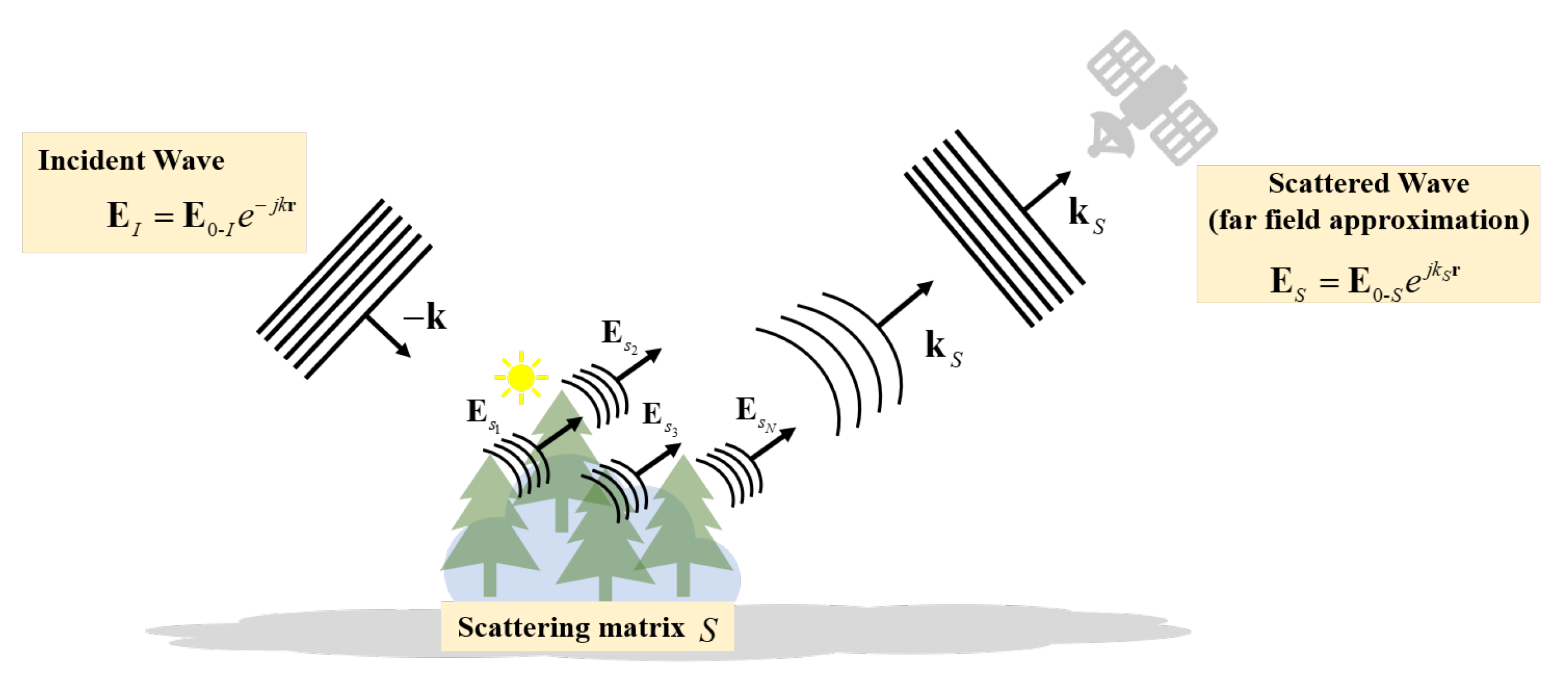
2.1.2. Scattering Matrix

PolSAR is one of the most important applications of PI in the field of RS. Different from OPI, PolSAR works in the microwave band instead of the visible band. It is necessary to introduce the parameters used in PolSAR-based RS. Figure 4 presents a scheme of general PolSAR used to measure a target, characterized by its scattering matrix S [46].

Any electromagnetic wave’s polarization state can be determined by combining two orthogonal Jones vectors linearly [46]. As a PolSAR sensor transmits the horizontally (H) and vertically (V) polarized microwave alternately, while receives independently the returning H and V waves back-scattered in targets [139], the scattering process occurring at the target (shown in Figure 4) is expressed by using the scatter matrix S, whose foundation is same to the Jones matrix in OPI systems shown in Equation (2) and that characterises the coherent scattering of electromagnetic waves. The Scatter matrix is defined as follows:

$${\mathbf{E}}_I=S·{\mathbf{E}}_S=\left[\begin{array}{cc}{S}_{HH}& S_{HV}\\ S_{VH}& S_{VV}\end{array}\right]{\mathbf{E}}_S,$$

(6)

where the incident and the scattered waves are represented by ${\mathbf{E}}_I$ and ${\mathbf{E}}_S$, respectively. $S_{HH}$ and $S_{VV}$ related to the returned powers in co-polarized channels, while $S_{HV}$ and $S_{VH}$ are in cross-polarized channels. In particular, $S_{HV}$ is the scattering element of the horizontal transmitting and vertical receiving polarization, with $S_{HV}=\left|S_{HV}\right|e^{j{\varphi }_{HV}}$; Similar definition for $S_{VH}$. When reciprocal back-scattering, $S_{HV}=S_{VH}$ [133,134].

The covariance matrix or coherence matrix is another important parameter commonly used in PolSAR data processing [46,140]. It is defined in the following way. One first “vectorizes” the scattering matrix S and defines the 3D scattering vector below

$$\mathbf{X}={[S_{HH},\sqrt{2}{S}_{HV},S_{VV}]}^T,$$

(7)

under the assumption of $S_{HV}=S_{VH}$. One then defines the covariance matrix as the average of the outer product of $\mathbf{X}$ as $C=〈\mathbf{X}{\mathbf{X}}^H〉$ [140]:

$$\left[\begin{array}{ccc}〈{\left|S_{HH}\right|}^2〉& \sqrt{2}〈S_{HH}{S}_{H{V}^{\ast }}〉& 〈S_{HH}{S}_{VV}^{\ast }〉\\ \sqrt{2}〈S_{HV}{S}_{H{H}^{\ast }}〉& 2〈{\left|S_{HV}\right|}^2〉& \sqrt{2}〈S_{HV}{S}_{VV}^{\ast }〉\\ 〈S_{VV}{S}_{H{H}^{\ast }}〉& \sqrt{2}〈S_{VV}{S}_{H{V}^{\ast }}〉& 〈{\left|S_{VV}\right|}^2〉\end{array}\right],$$

(8)

where the averaging, i.e., $〈·〉$, involved in the computation of the covariance matrix can be temporal or spatial. For example, to suppress speckle noises in PolSAR images, one can average on several acquisitions (or “looks”):

$$\langle C\rangle =\frac{1}{L}\sum _{i=1}^L{x}_i{x}_i^{\mathrm{H}}=\left[\begin{array}{ccc}{C}_{11}\hfill & C_{12}\hfill & C_{13}\hfill \\ C_{21}\hfill & C_{22}\hfill & C_{23}\hfill \\ C_{31}\hfill & C_{32}\hfill & C_{33}\hfill \end{array}\right],$$

(9)

where L denotes the number of looks, $x_i$ the scattering vector of the i-th look. According to Equation (8), one knows that the principal diagonal elements in $\langle C\rangle$ are real-valued; the others are complex-valued and verify $C_{ij}=C_{ji}^{\ast }$, with $i\ne j$ [141].

As C includes all polarization information of targets, one can obtain useful features by decomposing this matrix [142]. Up to now, many decomposition algorithms have been developed to achieve this purpose, such as (1) the coherent decomposition algorithms including Krogager [143] and Target Scattering Vector Model [144]; and (2) the non-coherent decomposition algorithms including Holm [145], Huynen [146], Vanzyl [147], $H/A/\alpha$ [148], multiple component scattering model [149], Freeman [150], and adaptive non-negative eigenvalue decomposition [151].

2.2. Overview of Deep Learning

Neural networks are inspired by mammal brains and primate visual systems in particular, which comprise neurons or units with certain activation parameters by a deep architecture. In this way, a given input percept can be represented at multiple levels of abstraction [111,152]. DL, as a class of neural network-based learning algorithms, is composed of multiple layers, which are often referred to as ”hidden.” These layers transform the input into the output by learning progressively higher-level features. Notably, the network depth is typically dependent on the number of multiple hidden. This is why we always named the network “deep learning”.

In recent years, various novel deep architectures have been developed and applied in various fields, where they outperform the traditional non-data-driven methods [110,116,153,154]. We still take the ALOS-2/PALSAR as an example. Ref. [155] proposed a DL-based approach and achieved robust operational deforestation detection with false alarm rate smaller 15%, as well as improved the accuracy by 100% in some areas. In this Section, we will introduce several DL models commonly used in PIs, e.g., the convolutional neural networks (CNN), autoencoders (AE), and deep belief networks (DBN) [116,152,153,156,157,158].

2.2.1. CNN

The concept of CNN was proposed by [159] and then revised by [160]. In the past decades, CNN has attracted more attention and shown outstanding performance in various fields including, but not limited to, optical sensing [161,162] and imaging [163,164]. CNN has the prominent ability to learn highly abstract features and is a trainable multi-layer architecture composed of an input layer, convolutional layers, pooling layers, fully connected layers, and an output layer [165]. One example of the CNN architecture is shown in Figure 5.

Convolutional layer is used to extract image features. The former convolutional layers aim at extracting shallow features, while latter ones aim to further learning abstract features. The convolutional layer computes output multiple feature maps by convoluting the output of the previous layer (or input layer) with a convolution kernel [166,167,168].

Pooling layer aims at reducing the size of the input (former) layer by, for example, sampling convolved feature maps. By this way, useful features of the image are preserved and redundant information is removed, thus effectively preventing the over-fitting problem and speeding up computation [115,158].

Fully connected layer combines features transmitted in the former layers to achieve the final feature representation. It is always used in the last layer and followed by the output layer.

In addition, to boost the performance, many CNN models have been proposed, including the LeNet [169], AlexNet [163], GoogleNet [170], ResNet [171], DenseNet [172]. Notably, CNNs have been widely used in PIs, for such applications as image reconstruction [5,11,58], target recognition [173,174,175], classification for PolSAR data [49,176]. We will introduce these works in Section 3.

2.2.2. AE

AE is a symmetrical neural network composed of two connected networks: encoder and decoder. Its architecture is shown in Figure 6. The two parts can be considered as hidden layers between the input and output layers [177].

In the first encoder part, input data, which always has a high dimension, was reduced to low-dimensional encoded data. During this part, the input data $x_i$ is processed by a linear function and a NAF f to provide encoded data $y_i$. On the contrary, the decoder part raises the encoded data to a reconstructed data $x_i^r$, having the same dimension as $x_i$. The network is optimized by minimizing the loss function, for example, with a back-propagation algorithm, AE learns features from the input in an unsupervised way.

Many variants of AE have been developed to boost the performance according to special applications, such as the sparse AE [177], convolutional AE [178], and variational AE [179]. In fact, these AEs can be directly employed as the feature extractor from polarization images, for example, in target detection and classification for PolSAR data [180,181,182,183,184].

2.2.3. DBN

DBN is an unsupervised probabilistic network [185]. It stacks multi-individual unsupervised networks whose hidden layer is used as the input for the next layer. Usually, DBN comprises the stacking of several Restricted Boltzmann Machines (RBMs) or AEs. DBN has two layers: the hidden layer and the visible layer. Hidden units are conditionally independent of visible ones. Its architecture is shown in Figure 7 [43,111,185].

DBN-based methods have been used in PI applications, especially the object recognition and scene classification [186,187,188,189], and have shown superior performance compared with traditional methods, such as PCA [181] and support vector machines (SVM) [190].

2.2.4. Other Deep Networks

In addition to the above three network models, a few research works in the field of PI are based on other late-model networks, such as the recurrent neural network (RNN) [191,192], generative adversarial network (GAN) [97], residual network [5], and deep stacking network (DSN) [193].

As a typical neural network, RNN uses a loop to store information within the network. This gives the network a memory capacity to preserve information. The current input and prior hidden states are used to compute a new hidden state, as $h_t=f\left(h_{t-1},x_t;W\right)$; where $h_t$ and $h_{t-1}$ are hidden states at time t and $t-1$, respectively; $x_t$ denotes the present input; W is the parameter applied in all time sequences; and f denotes a NAF. Figure 8 presents an example of RNN architecture.

It can be seen that, in contrast with previously introduced networks, RNN provides a feedback loop to previous layers. The advantage of RNN over the feed-forward networks is that it can remember the output and use it to predict the next elements, while the feed-forward one is not able to feed the output back to the network. Therefore, RNN works very well with sequential data. The RNN with gated recurrent unit and the Long Short-Term Memory (LSTM) are two of the most often used RNNs (GRU). They solve problems of vanishing or exploding gradient [121,194], and have been successfully used to handle the classification issues in PolSAR [191,192].

GAN is a class of DL systems developed by [195]. It contains Generator (G) and Discriminator (D), i.e., two sub-networks. The GAN training algorithm involves training both the G and D models in parallel, and having them compete against one another in a zero-sum game. Figure 9 presents an example of GAN architecture.

In other words, “G” tries to mislead “D” into distinguishing between the true and fake. “D” is trained to recognize that information is true whenever it comes from a reliable source and is false when it comes from “G”. GANs are now a very active research topic in image processing applications, and there exist various types of GANs, such as Vanilla GAN, conditional GAN (CGAN), WGAN, StyleGAN, deep convolutional generative adversarial network (DCGAN) [196,197,198].

In fact, due to the well-known vanishing gradient problem, deep networks are actually challenging to train. In other words, when the gradient propagates back to earlier layers, repeated multiplications may reduce it to an endlessly small value, saturating the performance or even rapidly decreasing it as the network depth increases. To handle this problem, Ref. [165] proposed ResNet, short for Residual Network, in 2015. The key of ResNet is to create an “identity shortcut connection” that skips one or more layers, which is called a “residual block” and is depicted on the left-side of Figure 10.

The ResNet is robust to exploding and vanishing gradients as residual blocks can pass signals directly through, which allows information to be propagated faithfully among multi-layers. Thanks to its excellent performance, the ResNet has become one of the most popular architectures and has successfully been applied in many applications [5,11,165].

To further make use of shortcut connections and connect all layers directly with one another, in 2016, Ref. [172] proposed a novel architecture called Densely Connected network (DensNet) (As shown on the right of Figure 10). The figure shows that each layer’s input consists of all earlier layers’ feature maps, and the related outputs are passed to the subsequent layer. This operation makes networks highly parameter-efficient. In practice, one can always get better performance with fewer layers. DensNet can also be combined with the Resnet, the so-called Residual Dense Network, to further improve image quality in PI systems for such tasks as super-resolution [199], denoising [5] and dehazing [78].

3. PI via Deep Learning

The performance of DL-based methods depends on the learned relations between inputs and outputs. For polarization information acquisition, one needs to obtain a database of intensity images in multi-channels corresponding to different physical or polarimetric realizations of targets. Depending on the practical applications at hand, the detecting instrument may be the traditional Stokes imager [200], Mueller ellipsometer [201], or PolSAR [151]. The DL structures are specially designed to enhance the quality of these outputs by adding physical constraints. The outputs can be intensity images in different channels or the corresponding polarization parameters presented in Figure 2.

The captured polarization information may become the input of the second step of PI, i.e., polarization information applications. In other words, the second step is based on the outputs of the first step, and its output nature depends on the task at hand. For example, it can be a denoised image in denoising/despeckling applications, a clear image in haze and cloud removal, and a feature map in object classification and detection.

Based on captured polarization dataset, physical relations between inputs and outputs can be learned by adjusting connection weights and other parameters of the DNN structure. Consequently, data-driven approaches effectively seek and handle polarimetric information with high imaging performance [5,11,43,58]. Besides, compared with traditional solutions, PI using DL-based solutions are also very fast because it is a feed-forward architecture [121,168,202]. Recently, some researchers have tried to develop DNNs that embed physical priors, models, and constraints into, for example, the forward operators, regularizers, and loss functions [5,11,168,174]. They have verified that such DNNs have significant superiority compared with those that do not consider physical priors.

In the following two sections, we will review DL-based methods for improving the performance of PI in terms of acquisition and application, respectively. A brief outline of these Sections is shown in Figure 11. Specifically, we will introduce a series of representative DL-based works in polarization applications and processing, respectively, and show how DL enhances the PolSAR and OPI.

4. Polarization Information Acquisition

In some scenes, polarimetric images could suffer from the noise, speckles, haze, clouds, or reduced resolution, which compresses their quality and limits practical applications. Employing DL at the level of PI acquisition can significantly improve image quality thanks to the power of data-driven methods and their ability to extract features.

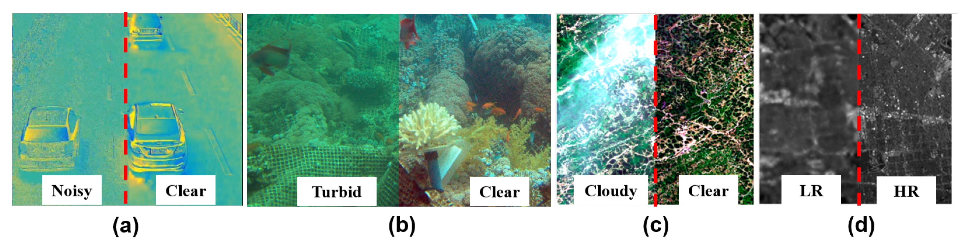
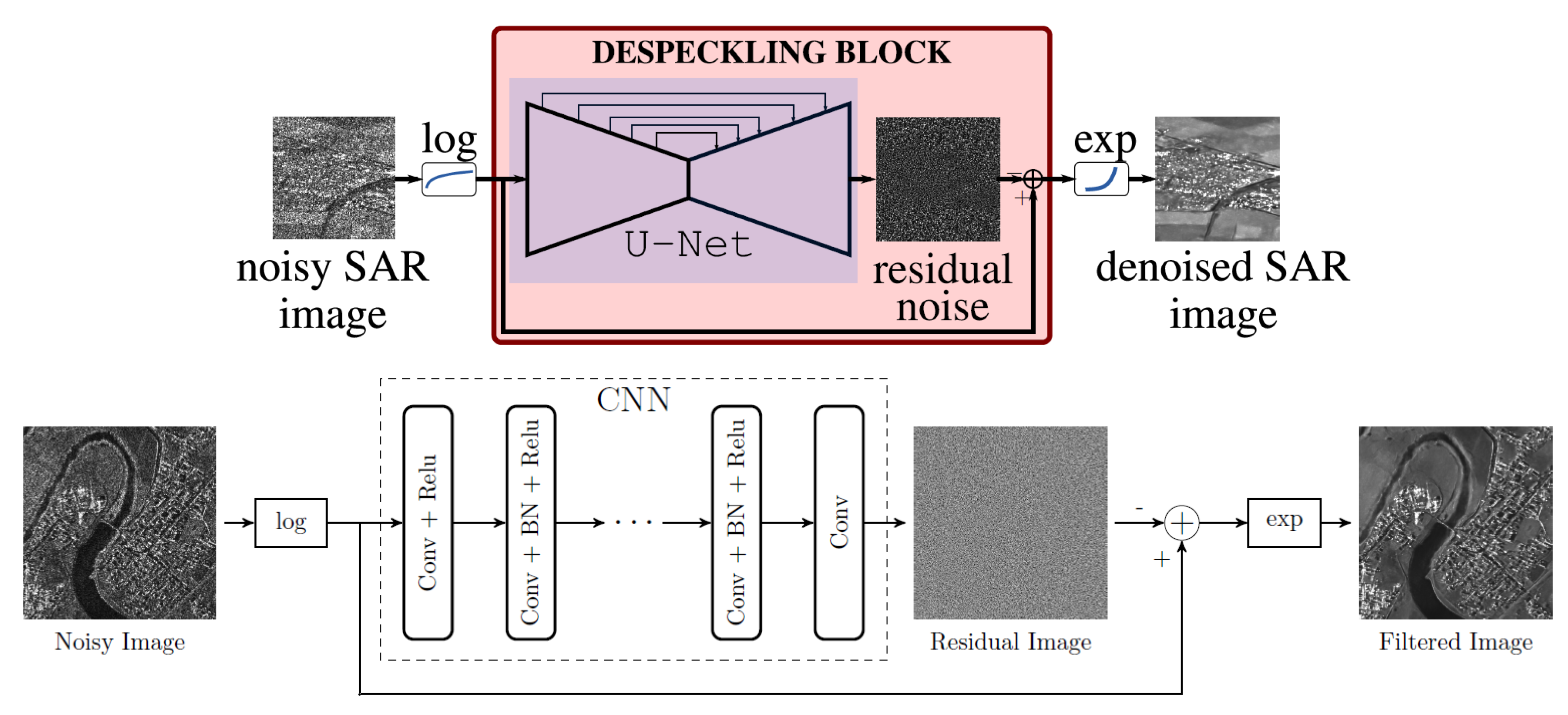
4.1. Denosing and Despeckling

PI aims to measure and image polarization parameters and has been widely applied to many fields. Yet, essential polarization parameters are deduced by intensities or powers via nonlinear operators, which could magnify the noise distorting intensity/power measurements [203,204]. As such, they are quite sensitive to the noise. This is illustrated on the left of Figure 12, where details in noisy DoLP/AoP images are challenging to distinguish [5,205]. In RS, the speckle noise is one of the leading reasons for SAR data quality reduction. Additionally, PolSAR data has a far more complex speckle model than conventional SAR data. This is due to the fact that the speckle noise can be seen both in intensity images and in complex cross-products between various polarization parameters [69,79]. Figure 12 (Right) presents the illustration of non-stationary speckles in a PolSAR image (F-SAR airborne image DLR). As the radiometry and polarimetric behaviors differ, the two enlarged regions appear at different noise levels, making speckles removal more difficult [206].

4.1.1. PI Case

In visible PIs, many non-data-driven denoising methods have been proposed and generally shown positive performances. For instance, Ref. [106] proposed a PCA-based denoising method that fully takes advantage of the spatial connection between various polarization states. To specifically suppress noise, two crucial processes—dimensionality reduction and linear least mean squared-error estimation in the transformed domain—are used. In 2018, Ref. [207] proposed a novel K-SVD-based denoising algorithm for polarization imagers. This algorithm can efficiently eliminate Gaussian noise and well-preserve the targets’ details and edges. In addition, BM3D-based denoising methods have also been employed to handle polarimetric images [109,208] and well preserve the details and edges of these images. However, they have two drawbacks: (1) the type of noise is assumed as additive white Gaussian, while the practical type may be more complex and will be affected by many factors; in other words, the methods can not well address practical applications. (2) Most methods rely on prior knowledge and need human structure parameter tuning; as a result, they are not solid for different conditions [5].

DL methods perform particularly well in various fields thanks to their excellent abilities in extracting features. They are more effective for image denoising or despeckling in complex and strong noisy environments than others. In 2020, Ref. [5] proposed a residual dense network-based denoising method. Its structure is shown on the left side of Figure 13a. This network considers a multi-channel polarization image input and outputs the corresponding residual image. Figure 13(a-3) presents denoising results for different polarization parameters (i.e., intensity, DoLP, and AoP) by varying methods (i.e., the PCA, BM3D, and the proposed DL-based solution). Obviously, the DL-based one has the best performance for all polarization parameters, and all image details are well restored. Especially for such details in AoP images, the noise seems to be removed significantly. Moreover, the efficiency of this method on different materials has been verified. This is the first report about denoising for PI using DL.

As the low photon count, polarimetric images captured in a low-light environment always suffer from strong noises, resulting in low image quality, affecting the accuracy of object detection and recognition [73,209,210]. Therefore, denoising in low-light conditions is another essential task for visible PIs. In 2020, Ref. [11] first collected a chromatic polarimetric image dataset and proposed a three-branches (intensity, DoLP, and AoP) network, called IPLNet, to improve the quality of both polarization and intensity images.

In contrast with the network developed in their previous work [5], the present one has two sub-networks, i.e., RGB-Net and Polar-Net. An RGB feature map is produced using the RGB-Net. The features above are divided into three different channels, followed by the Polar-Net, which aims to predict polarization information. Besides, a polarization-related loss function is well designed to balance the intensity and polarization features in the whole network. Indoor and outdoor (see Figure 13b) experiments were performed to verify its effectiveness. The corresponding models and results can be extended to automatic drive directly to enhance target recognition accuracy in complex conditions further. In 2022, Ref. [211] proposed an attention-based CNN for PI denoising. In this work, a channel attention mechanism is applied to extract polarization features by adjusting the contributions of channels. Another interesting contribution of this work is its adaptive polarization loss, which makes the CNN focus on polarization information.

4.1.2. RS Case

In RS, various methods aim to suppress speckle noises, e.g., multi-look processing [212], filtering [213,214], wavelet-based despeckling, BM3D algorithm [215] and TV methods [216]. These PolSAR speckle filters are based on the traditional adaptive spatial domain filters proposed by [45,213,214]. Besides, although the NLM-filter was initially developed to remove the noise in traditional digital images [217], it was successfully expanded to denoise PolSAR images recently [105,218]. From 2014 to 2016, merging a Wishart fidelity term from the original PolSAR TV model with a non-local regularization term created for complex-valued fourth-order tensor data [104,216,219] innovatively developed TV-based methods for PolSAR despeckling. More details of these methods can be found in two representative reviews of PolSAR despeckling, i.e., Refs. [69,220]. However, the methods also have significant limitations: (1) Due to the nature of local processing, spatial linear filter approaches would be unable to completely preserve edges and features [61]; (2) NLM methods have a low computational efficiency of similar patch searching, which limits their applications. (3) Variational methods significantly depend on model parameters and are time-consuming. In general, these techniques occasionally fail to maintain sharp features in fields with complex textures or generate unwanted block artifacts in images with speckles [61].

In most traditional denoising methods for SAR images, a statistical model about the signal and speckle is necessary. To release it, some researchers extended DL approaches to SAR image despeckling [51,60,61,221,222]. Some of these methods are based on U-Net [221,222] and Residual-Net [61,223]. The corresponding network structure and denoising results are shown in Figure 14.

Notably, most DL-based despeckling methods are developed only for intensity-mode images. However, images captured from SAR polarimeters or interferometers have multiple channels and complex values, making the corresponding despeckling process more challenging [63,206,224]. In 2018, Ref. [206] first applied DNNs to despeckling in PolSAR images. It decomposes the complex-valued polarimetric and/or interferometric matrices into real-valued channels with a stabilized variance. And then, a DNN is applied, in an iteration way, until all channels are restored. The bottom part of Figure 15 presents a restoration result on an airborne image captured by the DLR’s ESAR sensor (image over Oberpfaffenhofen provided with PolSAR).

The despeckling of PolSAR images can be further developed by adding non-local post-processing into the CNN-based MULog method. In 2019, Ref. [225] designed a novel approach along this line. The first step is a network named MuLoG, using a matrix logarithm transform and a channel decorrelation step to iteratively remove noise in each channel. The patches obtained by the CNN step are filtered in the following step, i.e., non-local filtering, to smooth artifacts. The authors claimed that point-like artifacts in homogeneous areas are significantly reduced via the second step, which verifies that combining the non-local processing and the DL technique is a promising idea for despeckling [225]. In addition to these works, in 2021, Ref. [226] proposed a dual-complementary CNN network, which includes a sub-network to repair the structures and details of noisy RS images. By combining a wavelet transform operation with a shuffling operation to restore image structures and details, this solution can recover structural and textural details with a lower computational cost.

Although the DL technique is a dramatic solution to image denoising or despeckling, it usually needs vast datasets. Significantly, scenarios always suffer from different types of noises or speckles (e.g., the Gaussian, Poisson, sparse, etc.), and it is challenging to obtain enough data corresponding to the same scene but different types of noise. To handle this issue, in 2022, Ref. [227] proposed a user-friendly unsupervised hyperspectral images denoising solution under a deep image prior framework. Extensive experimental results demonstrate that the method can preserve image edges and remove different noises, including mixed types (e.g., Gaussian noise, sparse noise). Besides, as there are no processes of regularization and pre-training, it is more user-friendly than most existing ones.

4.2. Dehazing

As the backscattering light is partially polarized, PI is also an effective solution for restoring imaging in scattering media [28,29,35,58,78,228]. Utilizing polarization information makes it possible to effectively remove the backscattering light (this problem is also collectively known as dehazing) and extract target signals. Dating back to 2001, Ref. [35] originally suggested using the polarization relationship between two orthogonally polarized images and the object radiance to achieve hazy removal. Refs. [228,229] proposed to analyze the DoLP and AoP of backscattering to remove haze/veiling in scattering media. In 2018, Ref. [6] proposed a method combining computer vision and polarimetric analysis, and this method had a significant performance for gray-level image recovery in dense turbid media. However, in these traditional methods, the physical model of the underwater PI system is often simplified and thus different from an actual situation. For example, they consider that backscattering light’s DoP has a specific value and estimate it based on a small local background region [229,230]. This deviates from practical situations.

Applying DL for polarimetric dehazing/de-scattering is promising, especially when the scattering media are strong. In 2020, before proposing a dense network for underwater image recovery, Ref. [58] first built a dataset containing 140 groups of image pairs using a DoFP polarization camera. The upper part of Figure 16 shows the network structure. We can see that the input of Polarimetric-Net is a set of polarimetric images, while the Intensity-Net is based only on an intensity image. This design is used to verify the superiority of PI in haze removal. The recovered results by different methods are shown on the down part of Figure 16 for comparison. From the figure, the water is densely turbid, which results in an image of poor quality where the details are severely degraded. In sharp contrast, the image recovered by the method, labeled by Polarimetric-Net, is the best. The details, even the ruler’s scale, can be clearly seen. This is the first report about dehazing with polarimetric DL. The design and the main idea could easily be extended to RS cloud removal.

In 2022, to break the dependence on strictly paired images, Ref. [64] proposed an unsupervised polarimetric GAN for underwater-image recovery, and merged polarization losses into the network to boost details restoration. Results (as shown in Figure 17) demonstrate that it improves the PSNR value by an average of 3.4 dB, verifying the effectiveness and superiority in different imaging conditions. For the underwater color polarized images, Ref. [231] proposed a 3D-convolutional neural network to handle the color intensity information and polarization information. This network considers the relationships among different information and contains a well-designed polarization loss. Restoration results demonstrate that it can significantly improve image contrast, restore details, and solve color distortion. Besides, compared with the traditional network structure (i.e., 2D-Net in Figure 17c), this 3D-Net has a significant performance in avoiding artifacts.

4.3. Super Resolution

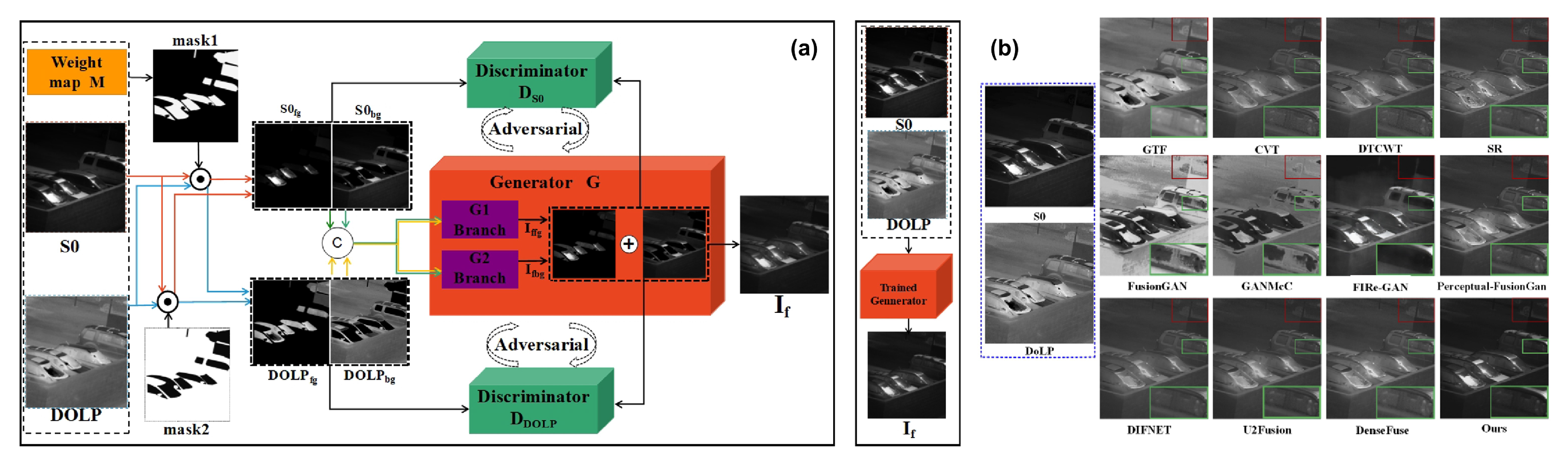
While capturing polarimetric images, the resolution may be reduced due to the limitation of detectors and optical systems. For example, DoFP polarimeters are frequently employed in visible PIs to acquire polarimetric data such as the Stokes vector, DoLP, and AoP in a single shot. This exceptional real-time performance is made possible by periodically integrated micro-polarizers on the focus plane; however, doing so lowers the spatial resolution. As a result, they affect the acquisition of the following polarization parameters.

Up to now, various interpolation algorithms have been developed to enhance resolution. This problem is also called demosaicing. The bilinear interpolation algorithm is one of the first two techniques utilized for DoFP imagers and has low computational complexity and accuracy. In contrast, the bicubic interpolation algorithm, though much more computationally intensive, achieves a reduced interpolation error in high contrast areas [232,233,234]. Recently, with the rise of interest for DL, Ref. [235] first proposed a CNN solution for polarization demosaicing, also named PDCNN. This technique divides the mosaicked polarization image into four channels, interpolates them using the bicubic approach, and then feeds the channels into a CNN that combines U-Net and skip connections. They compare the results with other methods for both DoLP and AoP images, which shows that the PDCNN outperforms the others by a large margin. This is the first report in the literature about DL-based demosaicing for PI.

The motivation of Zhang’s approach is to minimize the interpolation error of intensity-mode images with various polarization states. However, for a practical application, researchers really want to see such polarization parameters as intensity, DoLP, and AoP. For this purpose, Fork-Net, a four-layer, end-to-end completely CNN that [234] introduced, attempts to enhance the image quality of the tree parameters ($S_0$, DoLP, and AoP). Its architecture is simple and it allows for direct map relations between polarization features and mosaicked images. This architecture ensures a coherent optimization strategy and prevents accumulation errors from the stepwise method, which first captures various polarization orientations before computing the DoLP and AoP. In addition, they also designed a customized loss function with a variance constraint to guide network training.

Table 1. The PSNRs for Different Methods on Test Set.

	Bicubic	Correlation-Based	PDCNN	Fork-Net
$S_0$	38.0604	42.1540	42.9584	43.7225
DoLP	31.7751	29.8021	34.5301	35.0061
AoP	9.3744	7.6640	9.8273	11.0450

compares average PSNRs of images produced by different methods. One can see that this network realizes the highest quality of $S_0$, DoLP, and AoP estimation.

Subsequently, Ref. [236] extended this method to the case of chromatic polarimetric images and proposed a color polarization demosaicing network, named CPDNet, to jointly handle RGB and polarization image demosaicing issues. In 2019, Ref. [212] presented a conditional generative adversarial network (cGAN) architecture-based. In this network, the generator’s architecture is a U-Net, and the discriminator is based on a $64\times 64$ PatchGAN. To encourage physically realizable and accurate demosaiced images, they introduced physics-based constraints and Stokes-related losses into loss functions. The performance of this DL-based method for PI, which lacks ground truth, is comparable to that of methods that rely on ground truth. In 2022, Ref. [22] proposed a new AoP loss calculation method and applied it to a well-designed color polarization demosaicking network. This network contains multi-branch and has an increased convergence speed, i.e., three times compared with networks with the traditional AoP calculation method. This benefits from the fact that the AoP calculation method solves the “discontinuity” problem at $s_2=0$, thus effectively shortens the network’s optimization paths. We must note that the demosicing is not the total of resolution enhancement because that the reduced resolution of images comes from not only down-sampling, but also the effects of blurring and noisy. In 2023, Ref. [237] considered the fact and designed two models, i.e., “down-sampling” and “down-sampling + blurring + noisy”, and developed a residual dense network-based polarization super resolution solution. Compared to other methods, the method can well restored details of polarization images with a resolution-reduction factor of four.

All the above models and methods can also be directly applied to the resolution enhancement of PolSAR images. PolSAR images sacrifice spatial resolution for more accurate polarization information [46]. This lower resolution may be a limit in some applications, so it is necessary to improve spatial resolution [82,238]. When considering polarimetric channel information, one can obtain a robust reconstruction result, but the process is complex, as well as relationships between different channels are also relatively complicated as the special imaging mode in a coherent superposition of echoes [239]. In other words, it is hard to linearly fit relationships between different polarization channels [82]. It makes the resolution enhancement of PolSAR images more difficult.

Although CNN-based methods have been widely used for despeckling PolSAR images [82,240,241], techniques for improving resolution have yet to be considered. In 2020, Ref. [82] opened this door and proposed a residual CNN for PolSAR image super-resolution. It is the first CNN-based method used to improve PolSAR images’ resolution. The method improves spatial resolution and keeps detailed information, as shown in Figure 18.

Compared with traditional methods, the mean PSNR value is improved by up to 12%. In 2021, Ref. [244] proposed a fusion network to produce high-resolution PolSAR images based on fully PolSAR images and single-polarization synthetic aperture radar (SinSAR) images. This network developed a cross-attention mechanism to extract features while taking into account the polarization information of low-resolution PolSAR images and the spatial information of high-resolution single-polarization SAR images. Average PSNR values are increased by 3.6 dB, while MAE values are reduced by 0.07.

4.4. Image Fusion

Image fusion or multi-modal image fusion is another critical step to boost applications, e.g., the detection and classification [245]. It consists of registering images acquired with different imaging modalities. For example, RS aims to obtain data simultaneously with high spectral and spatial resolutions. PolSAR data are the first choice for classification tasks because they can characterize geometric and dielectric properties of scatters [46,246,247]. Therefore, fusing the two data sources, i.e., the hyperspectral and PolSAR images, is of great interest and has high potential application [248].

There are many traditional examples of multi-data sources fusion for RS applications. For example, multispectral and panchromatic image fusion [245,249,250], hyperspectral and multispectral image fusion, hyperspectral and polarimetric image fusion [52,251,252,253]. In particular, for the classification of land cover using PolSAR and hyperspectral data, Ref. [254] developed a hierarchical fusion technique. To be more precise, the hyperspectral data are first utilized to discriminate between vegetation and non-vegetation areas, while the PolSAR data classify non-vegetation areas into manufactured objects, water, or bare soil. Ref. [255] fused PolSAR and hyperspectral data, and a features concatenation was produced by concatenating the hyperspectral data’s features. Then, decision fusion is used to combine the classification results from multiple classifiers. Ref. [256] used the two data sources to detect oil spills. Recently, extending DL methods to RS data fusion has become a hot topic [248,257]. Next, we will introduce some typical examples.

For the question of how to extract features and fuse hyperspectral images and PolSAR data, Ref. [52] proposed an effective solution, a two-stream CNN. For each data, this network generates identical but independent convolutional streams. The two streams are then combined with comparable dimensionalities inside a fusion layer. With this design, informative features from two data sources—namely, hyperspectral and PolSAR—are effectively extracted for fusion and classification purposes. Examples of classification results indicate that the CNN-based fusion approach may effectively extract features and fuse the complementary information from two data sources in a balanced manner.

In 2019, Ref. [97] proposed a generative-discriminative network, named PolNet, for fusing and classifying polarization and spatial features. A generative network and a discriminative network share the same bottom layers in this network. As a benefit, the problem of a finite number of labeled pixels in PolSAR applications can be effectively addressed. This design enables sharing labeled and unlabeled pixels from PolSAR images for training in a semisupervised manner. Additionally, the network informs a Gaussian random field prior and a conditional random field posterior on the learned fusion features and the output label configuration to increase fusion precision. By comparing the label maps and median overall accuracies (OAs), the authors found that the Pol-Net has the best accuracy among the list, and almost all pixels are well matched with ground truths visual quality. It should be noted that the PolSAR images used here are Flevoland.

Ref. [174] suggested using an unsupervised DNN to handle this problem. The suggested network, also known as PFNet, learns maps for fused intensity and DoLP images without using ground truths or complex activity level measurement and fusion rules. The best visual quality can be seen when comparing the PFNet to other approaches. In 2020, using CNN and a feature extractor to provide the distribution of polarization information, Ref. [90] proposed a polarization fusion approach. Experimental results demonstrate that the method can effectively extract polarization information; then, this information can improve the detection rate.

In 2022, Ref. [258] proposed a semantic-guided polarimetric fusion solution, which is based on a dual-discriminator GAN (i.e., SGPF-GAN). This network has a generator and two discriminators, as shown in Figure 19. The dual discriminator aims to identify the polarization/intensity of multiple semantic targets; and the generator’s objective is to construct a fused image by the weighted fusing of each semantic object image. Qualitative and quantitative evaluations verify the superiority of both visual effects and quantitative metrics, as shown by the results of qualitative and quantitative evaluations. Additionally, the performance can be greatly improved by using this fusion approach to detect transparent, camouflaged hidden targets and image segmentation.

For underwater imaging, in 2022, Ref. [259] proposed a DL-based method that uses a multi-polarization fusion GAN-based solution to learn relationships between objects’ polarization and radiance information, and its network architecture is presented in Figure 20a. Compared with different methods (as shown in Figure 20b), we can observe that this method preserves more details of the foreground and background under turbid water.

5. Polarization Information Applications

Once high-quality polarimetric images have been obtained, various practical applications can be addressed, such as object detection [268,269], segmentation [270,271] and classification [95,96]. Employing deep learning with network architecture and constraints adapted to each application can help to extract useful polarimetric information and thus significantly improve the performance [116,119,121,123,126].

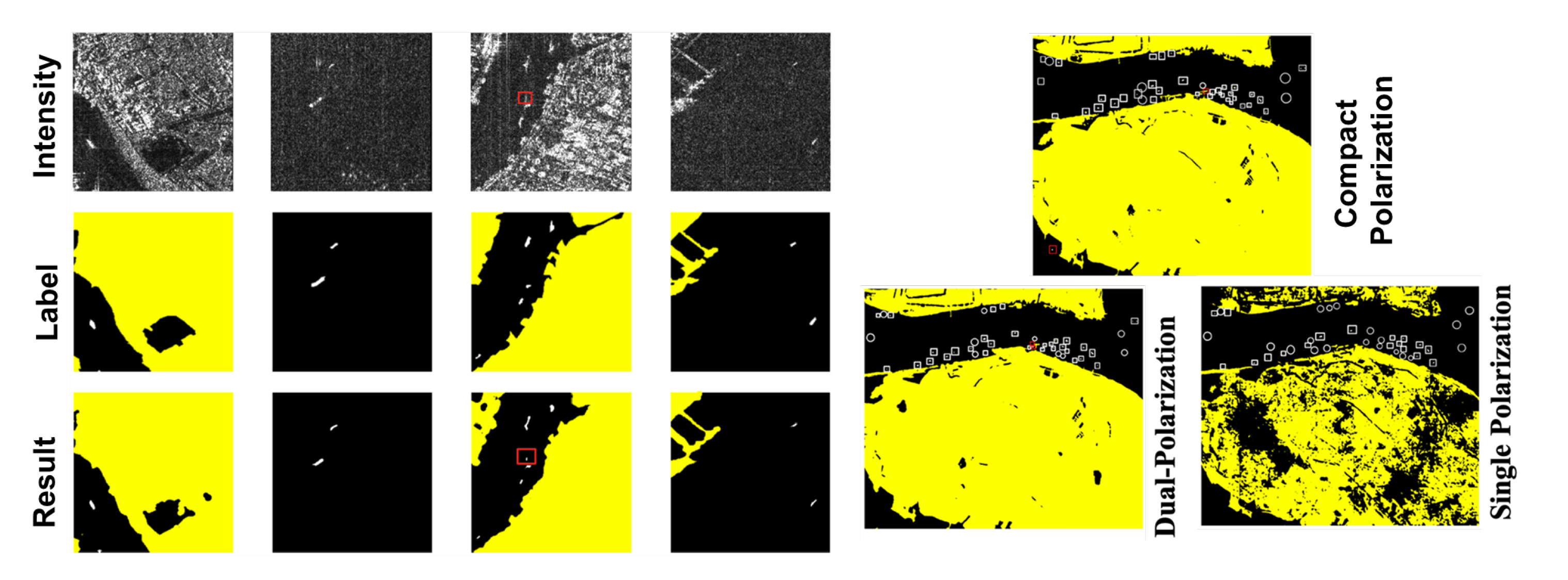
5.1. Object Detection

Polarization information can characterize important physical properties of objects, including geometric structures, material natures, and roughness, even under complex conditions with poor illumination or strong reflections. The fundamental idea behind polarization-encoded imaging is to identify the polarization characteristics of light that come from objects or scenes. Therefore, PI has significant application in object detection [4,46,268].

In visible imaging, as a fundamental task, road scene analysis plays an significant role, e.g., in autonomous vehicles, and advanced driver assistance systems. PI can provide generic features of the target objects under both good and adverse weather conditions [71,175,272]. For example, Ref. [175] explored the advantages of polarization parameters in discriminating objects and powerful of DNNs in extracting features to detect road scene contents in adverse conditions. By this way, detection tasks in adverse conditions (e.g., fog, rain, and low-light) were improved by about 27%.

In RS, PI and PolSAR have also shown to be effective methods for finding marine oil spills. The accuracy of conventional detection techniques depends on the quality of feature extraction, which is dependent on artificially derived polarization characteristics [256,273]. DL-based solutions are capable of automatically mining spatial features from data sets. For example, Ref. [273] developed an oil spill detection algorithm, which benefits from the multi-layer deep feature extraction by CNN. Figure 21 presents the flowchart of this algorithm. This figure shows how the PolSAR data (symmetrical $3\times 3$ complex coherency matrix) is first transformed into a nine-channel data block before being fed to the CNN. For the purpose of extracting two high-level features from the original data, it then constructs a five-layer CNN architecture. By using PCA and an SVM approach using a radial basis function kernel, the features dimension is reduced and merged. The comparison of the results of several approaches for spill detection is shown in Figure 21 (Down). The figure demonstrates how this technique can increase detection precision and successfully identify an oil spill from a biogenic slick.

Ship detection, one of the most significant RS applications, is crucial for commercial, fishing, vessel traffic service, and military applications [91,274,275,276]. In 2019, Ref. [91] proposed a pixel-wise detection method for compact polarimetric SAR (CPSAR) images based on a U-Net. It detects ships accurately both near and far away from the shore. However, false alarms can be generated by cross side-lobes. Examples of detection results are shown in the upper part of Figure 22. White and red rectangles refer to detected targets and false alarms, respectively, while white circles refer to missed targets. Compared with the Faster RCNN, the method has an increase of 6.54% and 8.28% in the indices of precision [277] and recall [277], which verifies the ability and advantages in detecting ships. This work also compares CPSAR images with other PolSAR modes such as single polarization and linear dual-polarization configurations, and shows that CPSAR is better at detecting ships, as shown in the bottom part of Figure 22.

Combining PI with DL can also be used for Change Detection (CD), such as urban change, sea ice change, and land cover/use change [92,173,278,279,280,281]. In 2018, Ref. [92] proposed a local restricted CNN for CD of PolSAR images. It can recognize not only different types of change but also reduce noise’s influence. Based on the multi-temporal PolSAR data, Ref. [278] developed a weakly supervised framework for urban CD. The technique achieves label aggregation in feature space using a multi-layer perceptron after learning multi-temporal polarimetric information using a modified unsupervised stacked AE stage. The authors test its efficacy and precision using an L-band UAVSAR dataset (in Los Angeles).

In 2020, Ref. [173] proposed a CNN Framework for the land cover/use CD in RS data from several sources. Three RS benchmark data are used to evaluate its efficiency and dependability (i.e., the multispectral, hyperspectral, and PolSAR). Examples and comparisons with several representative CD methods are shown in

Table 2. The accuracy of different change detection methods for the PolSAR-San Francisco dataset.

Method	CVA	MAD	PCA	IR-MAD	SFA	3D-CNN	Proposed
OA (%)	91.74	92.17	91.36	91.37	95.64	95.62	98.31
Sensitivity (%)	44.11	52.62	27.57	22.56	71.75	64.00	93.06
MD (%)	55.88	47.37	72.42	77.43	28.24	35.99	6.93
FA (%)	3.78	4.11	2.64	2.16	2.11	1.41	1.19
F1-Score (%)	47.85	53.58	35.41	30.98	73.88	71.49	90.43
BA (%)	70.16	74.25	62.46	60.19	84.82	81.29	95.93
Precision (%)	52.27	54.57	49.47	49.42	76.14	80.95	87.94
Specificity (%)	96.21	95.88	97.35	97.83	97.88	98.58	98.80
KC	0.434	0.493	0.311	0.271	0.715	0.691	0.895

. From the results, i.e., the first column of Table 2, all CD methods’ OA values are higher than 91%, but the proposed method’s OA is over 98%. In addition, the values of BA, sensitivity, and F1-Score are over 90%. The FA, MD, and precision of CD are also greatly improved compared with other methods. In 2021, Ref. [282] proposed a ship detection method for land-contained sea without a traditional sea-land segmentation process. This method includes two stages and can well-addressed the ship detection under complex conditions, i.e., an offshore area. Experimental results demonstrate that the accuracy and the F1 score can reach 99.4% and 0.99, respectively.

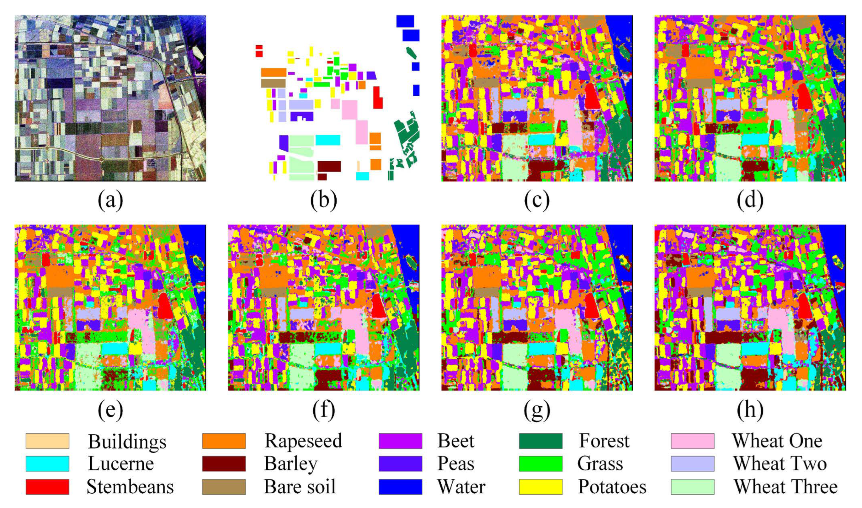
5.2. Target Classification

The classification tasks for SAR/PolSAR data are the most prioritized aspects for RI. Moreover, as PolSAR provides more information than other SAR systems, using polarization information obtained by PolSAR images can further improve classification accuracy and has many applications in oceanography, agriculture, forestry, and disaster monitoring [43,95,96,283,284]. Among these applications, classifying land use or cover in PolSAR images is one of the most challenging tasks. It mainly consists of different land classes, such as desert, lake, agricultural, forest, and urban [46,116]. Studies on PolSAR classification help understand different environmental elements and study the corresponding impact [285,286]. Figure 23 presents a general classification scenario [43].

In practice, one can perform classification processes based on multi-channel PolSAR or use specific parameters. Back in 2014, Shang and Hirose et al. have applied a neural-network-based technique named quaternion neural-network (QNN) to handle land classification [287,288,289,290]. Compared to methods at that time, the applied QNN method is effective and achieves higher classification performance because the used polarization parameters (e.g., Poincare-sphere-parameter [287,288] and Stokes vector [289]) are multidimensional. With the development of different but fruitful DL models, DL has successfully been used in classifying PolSAR data and well addressed the issue of big and multidimensional polarization data processing.

In 2016, Ref. [181] first designed an AE model for the task of terrain and achieved remarkable improvement in classification accuracy. Ref. [291] proposed a novel PolSAR terrain classification framework using deep CNNs. They used 6-D real-valued data, computed from the coherency matrix, to represent original PolSAR data, and naturally employed spatial information to perform terrain classification thanks to the power of CNN.

Table 3. Accuracy for the labeled area in the image of Flevoland.

Classes	Accuracy [%]	Classes	Accuracy [%]
0. Stembeans	92.58	8. Grasses	79.20
1. Peas	88.89	9. Rapeseed	93.10
2. Forest	93.95	10. Barly	96.90
3. Lucerne	92.21	11. Wheat2	91.82
4. Wheat	93.62	12. Wheat3	94.46
5. Beet	89.74	13. Water	98.88
6. Potatoes	87.24	14. Building	87.18
7. Bare soill	99.94	Overall	92.46

lists the accuracy for the labeled area in the image of Flevoland. From this table, we may observe that the overall accuracy for 15 classes reaches 92.46%. Ref. [292] found that in previous methods, as all PolSAR image’s pixels are classified independently, inherent interrelations of different land covers are always ignored. To solve this problem, they used a fixed-feature-size CNN, named FFS-CNN, to classify the pixels in a patch simultaneously; as a result, this solution is faster than other CNN-based methods.

Notably, these methods only consider the pixels’ amplitude; as a result, they cannot obtain enough discriminative features. In 2019, Ref. [140] designed a complex-valued convolutional auto-encoder network named CV-CAE. The phase information of PolSAR images could be utilized because all encoding and decoding operations are extended to the complex domain. To further improve performance, they also suggested a post-processing technique called spatial pixel-squares refinement. By calculating a blocky land cover structure, this method can increase refinement efficiency. Figure 24 presents the classification results and compares the performance of different algorithms. The intra-class smoothness and the inter-class distinctness outperform those of the compared algorithms.

Generally speaking, distinctions between PolSAR and OPI are rarely taken into account in published works. Since complex-valued PolSAR data are frequently converted to real-valued data to fit the OPI processing and prevent complex-valued operations, CNNs are typically not designed for PolSAR classification. This is one of the reasons CNNs are unable to utilize all of their capabilities when doing the PolSAR classification assignment [70]. To solve this problem, in 2019, Ref. [70] developed a CNN architecture specifically for PolSAR image classification. A crucial step in the processing is looking for better PolSAR data as the input. They suggested a multi-task CNN (MCNN) structure for the network architecture to fit the enhanced inputs; MCNN is made up of the interaction module, amplitude branch, and phase branch. They also added a depth-wise separable convolution, known as DMCNN, to MCNN in order to effectively model potential correlations from the PolSAR phase. Figure 25 compares classification performances of different methods. From this figure, we may find that the proposed methods, the improved DMCNN, in particular, reach a better level of terrain completeness in classification maps.

Recently, based on the C-band SAR, i.e., Gaofen-3 satellite with the dual-polarization state, i.e., VV and VH, in the western Arctic Ocean from January to February 2020), Ref. [294] designed a network framework aims to handle classification issue of the Arctic sea ice in winter. The results showed that, using two polarization states (i.e., VH + VV) improves the classification accuracy by 10.05% and 9.35%, respectively, compared with that only using VH or VV polarization.

An open question is how to apply PolSAR’s spatial and polarization information at the same time. DCNNs are able to produce high-level spatial features and achieve cutting-edge performance in image analysis because of their sophisticated designs and vast visual databases. However, because PolSAR data are multi-band and complex-valued, a standard model cannot be used to handle PolSAR data straightforwardly. Ref. [295] built a dataset to explore the abilities and DCNN’s potential on PolSAR classification. This work used six pseudo-color images (i.e., intensity, $C_{11}$, $C_{22}$, $C_{33}$, $C_{11}$, $H-\alpha -A$ decomposition image, and Yamaguchi decomposition image) to characterize one random sample in each category. By a transfer learning framework, which incorporates a polarimetric decomposition into a DCNN, taking spatial analytic ability into account, the framework’s validation accuracy ups to 99.5%. Ref. [296] proposed a Dual-CNN for PolSAR classification. The main procedures are displayed in Figure 26 and contain two deep CNNs: extracting polarization features from a coherency matrix deduced 6-channel real matrix (i.e., 6Ch), and extracting spatial features in Pauli RGB images. A fully connected layer combines all extracted polarization and spatial property features. And then, a softmax classifier is used to classify features. The results displayed in Figure 26b verify the effectiveness of combining 6Ch-CNN and PauliRGB-CNN via fully connected layers. They claim that the classification precision on 14 land cover types is 98.56%.

According to the type of PolSAR image datasets, i.e., whether prior data is needed, one can divide the classification into supervised and unsupervised methods. In contrast to the unsupervised one, which simply requires scattering and statistical distributions derived from PolSAR data, the supervised one requires human interaction to acquire previous knowledge. Recently, semi-supervised methods have attracted more attention for using labeled and a few unlabeled samples to handle limited training sets. For example, Ref. [184] proposed a super-pixel restrained DNN with multiple decisions (SRDNN-MDs). It extracts effective super-pixel spatial features and reduces speckles based on only a few samples. This method is a semi-supervised classification model and yields higher accuracy.

Further, to release the classification from prior knowledge, in 2021, Ref. [297] proposed an unsupervised classification network via a decomposition and large-scale spectral clustering method with super-pixels, also called ND-LSC. Figure 27 depicts the architecture, which mainly consists of two parts.

They first extracted polarization scattering parameters by a new decomposition (ND); it contributes to understanding the polarimetric scattering mechanisms of sandy land [297]. Then, to speed up the processing of PolSAR images, they used large-scale spectral clustering (LSC), which creates a bipartite graph. The solution is effective and adaptable for wide regions thanks to this design. They tested the efficacy of the approach using the RADARSAT-2 fully PolSAR dataset (Hunshandake Sandy Land in 2016), with an OA value of 95.22%. The detailed results and the corresponding comparison can be found in

Table 4. Confusion Matrix of the ND-I SC Method (PA: %; UA: %).

Class	HED-SC		ND-RF		ND-LSC
	PA	UA	PA	UA	PA	UA
RT	81.17	95.19	85.42	73.64	90.22	96.94
RD	89.05	64.51	91.35	68.69	98.75	95.45
SS	91.31	84.28	93.45	85.36	94.62	87.28
DL	87.82	89.64	86.19	90.39	93.21	87.13
SL	81.69	94.37	84.67	94.75	91.02	87.07
V	75.20	90.54	79.89	94.47	97.87	69.65
L	96.35	99.67	96.86	99.68	98.07	74.59
OA (%)	89.68		90.02		95.22
Kappa	0.8717		0.9205		0.9404

and Figure 27. In 2023, Ref. [284] developed a hybrid attention-based encoder–decoder fully convolutional network (HA-EDNet) to handle the PolSAR classification. The network input can be an arbitrary-size image and used a softmax attention module to boost the accuracy. Considering the insufficient number of labeled data, in 2023, Ref. [300] proposed a vision transformer-based framework (named PolSARFormer) by using 3D and 2D CNNs as feature extractors, as well as the local window attention. Extensive experimental results demonstrated that PolSARFormer got better classification accuracy than the state-of-the-art algorithms; for example, the results over the San Francisco data benchmark illustrated the accuracy improvement compared with the Swin Transformer (5.86%) and FNet (17.63%).

5.3. Others

In the above Sections, we mainly introduced examples of combining DL and PI in RS and some specific visible-wavelength applications. However, combining PI and DL can also be successfully used in other fields, such as biomedical imaging and computer vision [301,302,303,304].

For example, based on a trained deep CNN, Ref. [303], in 2021, found that holographic images can be reconstructed from a single polarization state via a single-shot computational polarization microscope. This work opens a new door for reconstructing multi-dimensional information from one-dimensional input. The main idea can be extended to other fields, such as road detection, to achieve real-time PI. In 2020, Ref. [305] proposed a Polarized CNN to handle the problem of transparent object segmentation and increase the corresponding accuracy. The top of Figure 28 shows the results.

Finally, to find effective solutions to the multi-species classification problems of algae, Ref. [304] proposed a Mueller system to classify morphologically similar algae via a CNN and achieved a 97% classification accuracy. This is the first report about the combination of PI and DL in marine biology. Besides, learning-based solutions can further improve the reconstruction accuracy of polarization-based 3D-reconstruction techniques. In 2022, a physics-informed CNN was designed to estimate the scene-level surface normal from a single polarization image. The corresponding indoor and outdoor experiments are presented at the bottom of Figure 28. This approach needs prior knowledge of viewing encoding to help address the increase of polarization ambiguities caused by complex materials and non-orthographic projection in the scene-level polarization shape [306]. Although these applications have large differences, the networks designed for polarization images in all these applications can learn from each other.

Finally, we summarize the reviewed works chronologically in Figure 29 to help the reader follow the chronological evolution of the methods and the different applications, as well as to find the target works as quickly as possible.

6. Conclusions

This paper have systematically reviewed advanced DL-based techniques for PI analysis. From two aspects of PI, i.e., the acquisition and the applications, we have shown that the DL-based methods have had significant success in such domains as denoising or despeckling, dehazing, super-resolution, object detection, fusion, and classification. In particular, depending on practical needs, different network models have been designed to handle each application. All the research works reviewed here can be considered strong evidence that DL-based PIs can break the limitations of traditional methods and provide irreplaceable solutions, especially for tasks in complex and hostile conditions. It’s worth noting that the reported DL models and researches largely depend on a special dataset, and it is difficult to guarantee similar performance for other datasets. This is the main disadvantage compared with other representative traditional models. Still, we always believe that the DL techniques are revolutionary in PIs.

In short, there is an excellent synergy between PI and DL techniques. DL boosts PI and vice versa. PI techniques and related applications enable DL since they constantly develop advanced systems to collect datasets, which is an essential part of DL development physically. Also, DL boosts PI since it enhances the capability and performance of optical technology in a data-learning way [307]. Many desired functions in both DL (e.g., small dataset, physical interpretation, and unsupervised) and PI (e.g., multi-data interaction, real-time process, and system simplified) techniques may be solved by reasonable integration [308,309,310,311,312], as shown in Figure 30. However, the research on the combination of PI and DL is still at the initial stage, and various key questions or directions remain unanswered and need consideration [116,121]. Some of these questions belong to the everyday problems of DL [122,308], and some are caused by the specificity of PI [93]. We list hereafter some potentially interesting topics in this field.

The number of training samples. Although DL-based models can learn hidden features from the polarimetric images or PolSAR data, their performance and accuracy extremely depend on the number of data available for training. In other words, the more data, the higher quality [308,309]. However, acquiring large datasets for PI systems is difficult, especially for practical applications in complex conditions, such as underwater/ocean images or high-resolution PolSAR data for RS. For example, in Li et al.’s work [5], the used dataset only contains 150 groups of full-size image pairs, and 140 groups in Hu et al.’s work [58]. In order to get enough data, they increase the dataset scale using a well-designed pixels window and flipping it horizontally or vertically with a fixed step of pixels. As a result, they obtained more than 100,000 images. This is indeed a compromise strategy. How to keep the considerable learning performance of DL approaches with fewer samples remains a significant challenge. This problem may be solved by introducing new network architecture, such as that based on transfer learning [309,311], or bound by solid physical and apriori knowledge [313,314,315].

The inherent limitations of PI systems. One needs to invert the acquired multi-intensity images to obtain the polarization information [75,78,85]. This time-consuming process makes it challenging to handle changing scenes in real-time. Although the pseudo-polarimetric method can take the corresponding tasks based on only a single sub-polarized image, such as the dehazing in Li et al.’s work [28], these methods are based on a model with physical approximation. Learning the relations between single-channel and multi-channel data and finding an efficient way to transform them is a possible solution. In the optical imaging fields, the DoFP polarization camera makes it possible to capture the linear Stokes vector in one shot. Yet, the image resolution is reduced due to the integrating pixels [316,317]. Compared with traditional resolution improvement methods, DL techniques may break the limitations of systems computationally [22,318,319].

Embedding physics in network models. DL models were originally derived from the field of computer vision and are thus adapted to input data consisting of a single image without any physical constraint. But in PIs, we have multi-images, and internal physical connections exist between them. Adding these physical connections or prior knowledge can boost networks’ ability [307,310,315,320,321,322]. How to add these physical constraints and where to add them needs to be investigated and balanced. Besides, most existing DL-based models need ground truth to guide the extraction of features and learning. Of course, some models can achieve this function in an unsupervised way, such as the GAN network, but the performance of these methods is limited and always significantly worse than the performance of supervised methods. How to further enhance, especially by adding prior physical knowledge into training, the performance of unsupervised solutions is a burning problem [64,227].

Image translation and fusion between PolSAR and OPI. PolSAR and OPI systems have essential differences in geometry and radiometry owing to varying instruments, wavelengths, and viewing perspectives [312,323,324,325,326,327]. Therefore, PolSAR data mainly characterize objects’ structural and dielectric properties. At the same time, OPI data contain spectral information [326,327,328]. Exploring PolSAR-to-OPI translation is beneficial for many applications, such as image interpretation, spatial information transfer, and cloud removal [329,330]; but this type of image translation is difficult to accomplish by a simple physical model [116,128,131,312]. Deep learning has the ability to simulate complicated relationships and maintain the advantages of both PolSAR and OPI techniques by performing image-to-image translation or fusion tasks [130,312,331].

This review only covers a part of representative works in PI; therefore, we encourage readers to review other relevant works further to get broader views. As more and more people are getting involved in working on the above topics, we believe that the age of “Big PI” will eventually come.

References

1. Bass, M.; Van Stryland, E.W.; Williams, D.R.; Wolfe, W.L. Handbook of Optics; McGraw-Hill: New York, NY, USA, 1995; Volume 2. [Google Scholar]
2. Tyson, R.K. Principles of Adaptive Optics; CRC Press: Boca Raton, FL, USA, 2015. [Google Scholar]
3. Fowles, G.R. Introduction to Modern Optics; Courier Corporation: North Chelmsford, MA, USA, 1989. [Google Scholar]
4. Goldstein, D.H. Polarized Light; CRC Press: Boca Raton, FL, USA, 2017. [Google Scholar]
5. Li, X.; Li, H.; Lin, Y.; Guo, J.; Yang, J.; Yue, H.; Li, K.; Li, C.; Cheng, Z.; Hu, H.; et al. Learning-based denoising for polarimetric images. Opt. Express 2020, 28, 16309–16321. [Google Scholar] [CrossRef] [PubMed]
6. Li, X.; Hu, H.; Zhao, L.; Wang, H.; Yu, Y.; Wu, L.; Liu, T. Polarimetric image recovery method combining histogram stretching for underwater imaging. Sci. Rep. 2018, 8, 1–10. [Google Scholar] [CrossRef] [PubMed]
7. Wang, H.; Hu, H.; Li, X.; Guan, Z.; Zhu, W.; Jiang, J.; Liu, K.; Liu, T. An angle of polarization (AoP) visualization method for DoFP polarization image sensors Based on three dimensional HSI color space. Sensors 2019, 19, 1713. [Google Scholar] [CrossRef] [PubMed] [Green Version]
8. Li, X.; Zhang, L.; Qi, P.; Zhu, Z.; Xu, J.; Liu, T.; Zhai, J.; Hu, H. Are indices of polarimetric purity excellent metrics for object identification in scattering media? Remote Sens. 2022, 14, 4148. [Google Scholar] [CrossRef]
9. Song, L.M.W.K.; Adler, D.G.; Conway, J.D.; Diehl, D.L.; Farraye, F.A.; Kantsevoy, S.V.; Kwon, R.; Mamula, P.; Rodriguez, B.; Shah, R.J.; et al. Narrow band imaging and multiband imaging. Gastrointest. Endosc. 2008, 67, 581–589. [Google Scholar] [CrossRef]
10. Zhao, Y.; Yi, C.; Kong, S.G.; Pan, Q.; Cheng, Y. Multi-band polarization imaging. In Multi-Band Polarization Imaging and Applications; Springer Berlin Heidelberg: Berlin/Heidelberg, Germany, 2016; pp. 47–71. [Google Scholar]
11. Hu, H.; Lin, Y.; Li, X.; Qi, P.; Liu, T. IPLNet: A neural network for intensity-polarization imaging in low light. Opt. Lett. 2020, 45, 6162–6165. [Google Scholar] [CrossRef]
12. Guan, Z.; Goudail, F.; Yu, M.; Li, X.; Han, Q.; Cheng, Z.; Hu, H.; Liu, T. Contrast optimization in broadband passive polarimetric imaging based on color camera. Opt. Express 2019, 27, 2444–2454. [Google Scholar] [CrossRef]
13. Hariharan, P. Optical Holography: Principles, Techniques, and Applications; Cambridge University Press: Cambridge, UK, 1998. [Google Scholar]
14. Kim, M.K. Full color natural light holographic camera. Opt. Express 2013, 21, 9636–9642. [Google Scholar] [CrossRef] [Green Version]
15. Levoy, M. Light fields and computational imaging. Computer 2006, 39, 46–55. [Google Scholar] [CrossRef]
16. Tyo, J.S.; Goldstein, D.L.; Chenault, D.B.; Shaw, J.A. Review of passive imaging polarimetry for remote sensing applications. Appl. Opt. 2006, 45, 5453–5469. [Google Scholar] [CrossRef] [Green Version]
17. Morio, J.; Refregier, P.; Goudail, F.; Dubois-Fernandez, P.C.; Dupuis, X. A characterization of Shannon entropy and Bhattacharyya measure of contrast in polarimetric and interferometric SAR image. Proc. IEEE 2009, 97, 1097–1108. [Google Scholar] [CrossRef]
18. Li, X.; Xu, J.; Zhang, L.; Hu, H.; Chen, S.C. Underwater image restoration via Stokes decomposition. Opt. Lett. 2022, 47, 2854–2857. [Google Scholar] [CrossRef]
19. Chen, W.; Yan, L.; Chandrasekar, V. Optical polarization remote sensing. Int. J. Remote Sens. 2020, 41, 4849–4852. [Google Scholar] [CrossRef] [Green Version]
20. Liu, T.; Guan, Z.; Li, X.; Cheng, Z.; Han, Y.; Yang, J.; Li, K.; Zhao, J.; Hu, H. Polarimetric underwater image recovery for color image with crosstalk compensation. Opt. Lasers Eng. 2020, 124, 105833. [Google Scholar] [CrossRef]
21. Meriaudeau, F.; Ferraton, M.; Stolz, C.; Morel, O.; Bigué, L. Polarization imaging for industrial inspection. Image Process. Mach. Vis. Appl. Int. Soc. Opt. Photonics 2008, 6813, 681308. [Google Scholar]
22. Liu, X.; Li, X.; Chen, S.C. Enhanced polarization demosaicking network via a precise angle of polarization loss calculation method. Opt. Lett. 2022, 47, 1065–1069. [Google Scholar] [CrossRef]
23. Li, X.; Han, Y.; Wang, H.; Liu, T.; Chen, S.C.; Hu, H. Polarimetric Imaging Through Scattering Media: A Review. Front. Phys. 2022, 10, 153. [Google Scholar] [CrossRef]
24. Cheng, G.; Xie, X.; Han, J.; Guo, L.; Xia, G.S. Remote sensing image scene classification meets deep learning: Challenges, methods, benchmarks, and opportunities. IEEE J. Sel. Top. Appl. Earth Obs. Remote Sens. 2020, 13, 3735–3756. [Google Scholar] [CrossRef]
25. Demos, S.; Alfano, R. Optical polarization imaging. Appl. Opt. 1997, 36, 150–155. [Google Scholar] [CrossRef]
26. Liu, Y.; York, T.; Akers, W.J.; Sudlow, G.P.; Gruev, V.; Achilefu, S. Complementary fluorescence-polarization microscopy using division-of-focal-plane polarization imaging sensor. J. Biomed. Opt. 2012, 17, 116001. [Google Scholar] [CrossRef] [Green Version]
27. Fade, J.; Panigrahi, S.; Carré, A.; Frein, L.; Hamel, C.; Bretenaker, F.; Ramachandran, H.; Alouini, M. Long-range polarimetric imaging through fog. Appl. Opt. 2014, 53, 3854–3865. [Google Scholar] [CrossRef] [PubMed] [Green Version]
28. Li, X.; Hu, H.; Zhao, L.; Wang, H.; Han, Q.; Cheng, Z.; Liu, T. Pseudo-polarimetric method for dense haze removal. IEEE Photonics J. 2019, 11, 6900611. [Google Scholar] [CrossRef]
29. Li, X.; Wang, H.; Hu, H.; Liu, T. Polarimetric underwater image recovery based on circularly polarized illumination and histogram stretching. In AOPC 2019: Optical Sensing and Imaging Technology; SPIE: Bellingham, WA, USA, 2019; Volume 11338, p. 113382O. [Google Scholar]
30. Zhanghao, K.; Chen, L.; Yang, X.S.; Wang, M.Y.; Jing, Z.L.; Han, H.B.; Zhang, M.Q.; Jin, D.; Gao, J.T.; Xi, P. Super-resolution dipole orientation mapping via polarization demodulation. Light. Sci. Appl. 2016, 5, e16166. [Google Scholar] [CrossRef] [PubMed]
31. Hao, X.; Kuang, C.; Wang, T.; Liu, X. Effects of polarization on the de-excitation dark focal spot in STED microscopy. J. Opt. 2010, 12, 115707. [Google Scholar] [CrossRef]
32. Li, X.; Goudail, F.; Chen, S.C. Self-calibration for Mueller polarimeters based on DoFP polarization imagers. Opt. Lett. 2022, 47, 1415–1418. [Google Scholar] [CrossRef]
33. Li, X.; Liu, W.; Goudail, F.; Chen, S.C. Optimal nonlinear Stokes–Mueller polarimetry for multi-photon processes. Opt. Lett. 2022, 47, 3287–3290. [Google Scholar] [CrossRef]
34. Goudail, F.; Terrier, P.; Takakura, Y.; Bigué, L.; Galland, F.; DeVlaminck, V. Target detection with a liquid-crystal-based passive Stokes polarimeter. Appl. Opt. 2004, 43, 274–282. [Google Scholar] [CrossRef] [Green Version]
35. Schechner, Y.Y.; Narasimhan, S.G.; Nayar, S.K. Instant dehazing of images using polarization. In Proceedings of the 2001 IEEE Computer Society Conference on Computer Vision and Pattern Recognition. CVPR 2001, Kauai, HI, USA, 8–14 December 2001; Volume 1, p. I. [Google Scholar]
36. Treibitz, T.; Schechner, Y.Y. Active polarization descattering. IEEE Trans. Pattern Anal. Mach. Intell. 2008, 31, 385–399. [Google Scholar] [CrossRef] [Green Version]
37. Schechner, Y.Y.; Narasimhan, S.G.; Nayar, S.K. Polarization-based vision through haze. Appl. Opt. 2003, 42, 511–525. [Google Scholar] [CrossRef]
38. Ghosh, N.; Vitkin, A.I. Tissue polarimetry: Concepts, challenges, applications, and outlook. J. Biomed. Opt. 2011, 16, 110801. [Google Scholar] [CrossRef] [Green Version]
39. Rehbinder, J.; Haddad, H.; Deby, S.; Teig, B.; Nazac, A.; Novikova, T.; Pierangelo, A.; Moreau, F. Ex vivo Mueller polarimetric imaging of the uterine cervix: A first statistical evaluation. J. Biomed. Opt. 2016, 21, 071113. [Google Scholar] [CrossRef] [Green Version]
40. Jacques, S.L.; Ramella-Roman, J.C.; Lee, K. Imaging skin pathology with polarized light. J. Biomed. Opt. 2002, 7, 329–340. [Google Scholar] [CrossRef]
41. Wang, W.; Lim, L.G.; Srivastava, S.; Bok-Yan So, J.; Shabbir, A.; Liu, Q. Investigation on the potential of Mueller matrix imaging for digital staining. J. Biophotonics 2016, 9, 364–375. [Google Scholar] [CrossRef]
42. Pierangelo, A.; Benali, A.; Antonelli, M.R.; Novikova, T.; Validire, P.; Gayet, B.; De Martino, A. Ex-vivo characterization of human colon cancer by Mueller polarimetric imaging. Opt. Express 2011, 19, 1582–1593. [Google Scholar] [CrossRef]
43. Parikh, H.; Patel, S.; Patel, V. Classification of SAR and PolSAR images using deep learning: A review. Int. J. Image Data Fusion 2020, 11, 1–32. [Google Scholar] [CrossRef]
44. Pierangelo, A.; Manhas, S.; Benali, A.; Fallet, C.; Totobenazara, J.L.; Antonelli, M.R.; Novikova, T.; Gayet, B.; De Martino, A.; Validire, P. Multispectral Mueller polarimetric imaging detecting residual cancer and cancer regression after neoadjuvant treatment for colorectal carcinomas. J. Biomed. Opt. 2013, 18, 046014. [Google Scholar] [CrossRef]
45. Lee, J.S.; Grunes, M.R.; De Grandi, G. Polarimetric SAR speckle filtering and its implication for classification. IEEE Trans. Geosci. Remote Sens. 1999, 37, 2363–2373. [Google Scholar]
46. Lee, J.S.; Pottier, E. Polarimetric Radar Imaging: From Basics to Applications; CRC Press: Boca Raton, FL, USA, 2017. [Google Scholar]
47. Yan, L.; Li, Y.; Chandrasekar, V.; Mortimer, H.; Peltoniemi, J.; Lin, Y. General review of optical polarization remote sensing. Int. J. Remote Sens. 2020, 41, 4853–4864. [Google Scholar] [CrossRef]
48. Mullissa, A.G.; Tolpekin, V.; Stein, A.; Perissin, D. Polarimetric differential SAR interferometry in an arid natural environment. Int. J. Appl. Earth Obs. Geoinf. 2017, 59, 9–18. [Google Scholar] [CrossRef]
49. Shang, R.; He, J.; Wang, J.; Xu, K.; Jiao, L.; Stolkin, R. Dense connection and depthwise separable convolution based CNN for polarimetric SAR image classification. Knowl.-Based Syst. 2020, 194, 105542. [Google Scholar] [CrossRef]
50. Pourshamsi, M.; Xia, J.; Yokoya, N.; Garcia, M.; Lavalle, M.; Pottier, E.; Balzter, H. Tropical forest canopy height estimation from combined polarimetric SAR and LiDAR using machine-learning. ISPRS J. Photogramm. Remote Sens. 2021, 172, 79–94. [Google Scholar] [CrossRef]
51. Yang, X.; Pan, T.; Yang, W.; Li, H.C. PolSAR image despeckling using trained models on single channel SAR images. In Proceedings of the 2019 6th Asia-Pacific Conference on Synthetic Aperture Radar (APSAR), Xiamen, China, 26–29 November 2019; pp. 1–4. [Google Scholar]
52. Hu, J.; Mou, L.; Schmitt, A.; Zhu, X.X. FusioNet: A two-stream convolutional neural network for urban scene classification using PolSAR and hyperspectral data. In Proceedings of the 2017 Joint Urban Remote Sensing Event (JURSE), Dubai, United Arab Emirates, 6–8 March 2017; pp. 1–4. [Google Scholar]
53. Ferro-Famil, L.; Pottier, E.; Lee, J.S. Unsupervised classification of multifrequency and fully polarimetric SAR images based on the H/A/Alpha-Wishart classifier. IEEE Trans. Geosci. Remote Sens. 2001, 39, 2332–2342. [Google Scholar] [CrossRef]
54. Singha, S.; Johansson, A.M.; Doulgeris, A.P. Robustness of SAR sea ice type classification across incidence angles and seasons at L-band. IEEE Trans. Geosci. Remote Sens. 2020, 59, 9941–9952. [Google Scholar] [CrossRef]
55. Pallotta, L.; Orlando, D. Polarimetric covariance eigenvalues classification in SAR images. IEEE Geosci. Remote Sens. Lett. 2018, 16, 746–750. [Google Scholar] [CrossRef]
56. Tadono, T.; Ohki, M.; Abe, T. Summary of natural disaster responses by the Advanced Land Observing Satellite-2 (ALOS-2). Int. Arch. Photogramm. Remote Sens. Spat. Inf. Sci. 2019, 42, 69–72. [Google Scholar] [CrossRef] [Green Version]
57. Natsuaki, R.; Hirose, A. L-Band SAR Interferometric Analysis for Flood Detection in Urban Area-a Case Study in 2015 Joso Flood, Japan. In Proceedings of the IGARSS 2018 IEEE International Geoscience and Remote Sensing Symposium, Valencia, Spain, 22–27 July 2018; pp. 6592–6595. [Google Scholar]
58. Hu, H.; Zhang, Y.; Li, X.; Lin, Y.; Cheng, Z.; Liu, T. Polarimetric underwater image recovery via deep learning. Opt. Lasers Eng. 2020, 133, 106152. [Google Scholar] [CrossRef]
59. Li, X.; Li, Z.; Feng, R.; Luo, S.; Zhang, C.; Jiang, M.; Shen, H. Generating high-quality and high-resolution seamless satellite imagery for large-scale urban regions. Remote Sens. 2020, 12, 81. [Google Scholar] [CrossRef] [Green Version]
60. Pan, T.; Peng, D.; Yang, W.; Li, H.C. A filter for SAR image despeckling using pre-trained convolutional neural network model. Remote Sens. 2019, 11, 2379. [Google Scholar] [CrossRef] [Green Version]
61. Zhang, Q.; Yuan, Q.; Li, J.; Yang, Z.; Ma, X. Learning a dilated residual network for SAR image despeckling. Remote Sens. 2018, 10, 196. [Google Scholar] [CrossRef] [Green Version]
62. Goudail, F. Noise minimization and equalization for Stokes polarimeters in the presence of signal-dependent Poisson shot noise. Opt. Lett. 2009, 34, 647–649. [Google Scholar] [CrossRef]
63. Denis, L.; Dalsasso, E.; Tupin, F. In Proceedings of the IEEE International Geoscience and Remote Sensing Symposium IGARSS, Brussels, Belgium, 11–16 July 2021; pp. 411–414.
64. Qi, P.; Li, X.; Han, Y.; Zhang, L.; Xu, J.; Cheng, Z.; Liu, T.; Zhai, J.; Hu, H. U2R-pGAN: Unpaired underwater-image recovery with polarimetric generative adversarial network. Opt. Lasers Eng. 2022, 157, 107112. [Google Scholar] [CrossRef]
65. Akiyama, K.; Ikeda, S.; Pleau, M.; Fish, V.L.; Tazaki, F.; Kuramochi, K.; Broderick, A.E.; Dexter, J.; Mościbrodzka, M.; Gowanlock, M.; et al. Superresolution full-polarimetric imaging for radio interferometry with sparse modeling. Astron. J. 2017, 153, 159. [Google Scholar] [CrossRef] [Green Version]
66. Ahmed, A.; Zhao, X.; Gruev, V.; Zhang, J.; Bermak, A. Residual interpolation for division of focal plane polarization image sensors. Opt. Express 2017, 25, 10651–10662. [Google Scholar] [CrossRef]
67. Tao, Y.; Muller, J.P. Super-resolution restoration of misr images using the ucl magigan system. Remote Sens. 2019, 11, 52. [Google Scholar] [CrossRef] [Green Version]
68. Goudail, F.; Bénière, A. Optimization of the contrast in polarimetric scalar images. Opt. Lett. 2009, 34, 1471–1473. [Google Scholar] [CrossRef] [Green Version]
69. Ma, X.; Wu, P.; Wu, Y.; Shen, H. A review on recent developments in fully polarimetric SAR image despeckling. IEEE J. Sel. Top. Appl. Earth Obs. Remote Sens. 2017, 11, 743–758. [Google Scholar] [CrossRef]
70. Zhang, L.; Dong, H.; Zou, B. Efficiently utilizing complex-valued PolSAR image data via a multi-task deep learning framework. ISPRS J. Photogramm. Remote Sens. 2019, 157, 59–72. [Google Scholar] [CrossRef] [Green Version]
71. Li, N.; Zhao, Y.; Pan, Q.; Kong, S.G.; Chan, J.C.W. Full-Time Monocular Road Detection Using Zero-Distribution Prior of Angle of Polarization. In Proceedings of the European Conference on Computer Vision, Glasgow, UK, 23–28 August 2020; Springer: Berlin/Heidelberg, Germany, 2020; pp. 457–473. [Google Scholar]
72. Dickson, C.N.; Wallace, A.M.; Kitchin, M.; Connor, B. Long-wave infrared polarimetric cluster-based vehicle detection. JOSA A 2015, 32, 2307–2315. [Google Scholar] [CrossRef]
73. Carnicer, A.; Javidi, B. Polarimetric 3D integral imaging in photon-starved conditions. Opt. Express 2015, 23, 6408–6417. [Google Scholar] [CrossRef] [Green Version]
74. Hagen, N.; Otani, Y. Stokes polarimeter performance: General noise model and analysis. Appl. Opt. 2018, 57, 4283–4296. [Google Scholar] [CrossRef]
75. Li, X.; Hu, H.; Liu, T.; Huang, B.; Song, Z. Optimal distribution of integration time for intensity measurements in degree of linear polarization polarimetry. Opt. Express 2016, 24, 7191–7200. [Google Scholar] [CrossRef] [PubMed]
76. Li, X.; Hu, H.; Wang, H.; Liu, T. Optimal Measurement Matrix of Partial Polarimeter for Measuring Ellipsometric Parameters with Eight Intensity Measurements. IEEE Access 2019, 7, 31494–31500. [Google Scholar] [CrossRef]
77. Goudail, F.; Li, X.; Boffety, M.; Roussel, S.; Liu, T.; Hu, H. Precision of retardance autocalibration in full-Stokes division-of-focal-plane imaging polarimeters. Opt. Lett. 2019, 44, 5410–5413. [Google Scholar] [CrossRef] [PubMed]
78. Hu, H.; Qi, P.; Li, X.; Cheng, Z.; Liu, T. Underwater imaging enhancement based on a polarization filter and histogram attenuation prior. J. Phys. D Appl. Phys. 2021, 54, 175102. [Google Scholar] [CrossRef]
79. Lopez-Martinez, C.; Fabregas, X. Polarimetric SAR speckle noise model. IEEE Trans. Geosci. Remote Sens. 2003, 41, 2232–2242. [Google Scholar] [CrossRef] [Green Version]
80. Jaffe, J.S. Computer modeling and the design of optimal underwater imaging systems. IEEE J. Ocean. Eng. 1990, 15, 101–111. [Google Scholar] [CrossRef]
81. Cariou, J.; Jeune, B.L.; Lotrian, J.; Guern, Y. Polarization effects of seawater and underwater targets. Appl. Opt. 1990, 29, 1689. [Google Scholar] [CrossRef]
82. Shen, H.; Lin, L.; Li, J.; Yuan, Q.; Zhao, L. A residual convolutional neural network for polarimetric SAR image super-resolution. ISPRS J. Photogramm. Remote Sens. 2020, 161, 90–108. [Google Scholar] [CrossRef]
83. Li, X.; Le Teurnier, B.; Boffety, M.; Liu, T.; Hu, H.; Goudail, F. Theory of autocalibration feasibility and precision in full Stokes polarization imagers. Opt. Express 2020, 28, 15268–15283. [Google Scholar] [CrossRef]
84. Li, X.; Hu, H.; Goudail, F.; Liu, T. Fundamental precision limits of full Stokes polarimeters based on DoFP polarization cameras for an arbitrary number of acquisitions. Opt. Express 2019, 27, 31261–31272. [Google Scholar] [CrossRef]
85. Li, X.; Goudail, F.; Hu, H.; Han, Q.; Cheng, Z.; Liu, T. Optimal ellipsometric parameter measurement strategies based on four intensity measurements in presence of additive Gaussian and Poisson noise. Opt. Express 2018, 26, 34529–34546. [Google Scholar] [CrossRef]
86. Li, X.; Hu, H.; Wang, H.; Wu, L.; Liu, T.G. Influence of noise statistics on optimizing the distribution of integration time for degree of linear polarization polarimetry. Opt. Eng. 2018, 57, 064110. [Google Scholar] [CrossRef]
87. Li, X.; Hu, H.; Wu, L.; Liu, T. Optimization of instrument matrix for Mueller matrix ellipsometry based on partial elements analysis of the Mueller matrix. Opt. Express 2017, 25, 18872–18884. [Google Scholar] [CrossRef]
88. Li, X.; Liu, T.; Huang, B.; Song, Z.; Hu, H. Optimal distribution of integration time for intensity measurements in Stokes polarimetry. Opt. Express 2015, 23, 27690–27699. [Google Scholar] [CrossRef]
89. Dubreuil, M.; Delrot, P.; Leonard, I.; Alfalou, A.; Brosseau, C.; Dogariu, A. Exploring underwater target detection by imaging polarimetry and correlation techniques. Appl. Opt. 2013, 52, 997–1005. [Google Scholar] [CrossRef]
90. Sun, R.; Sun, X.; Chen, F.; Pan, H.; Song, Q. An artificial target detection method combining a polarimetric feature extractor with deep convolutional neural networks. Int. J. Remote Sens. 2020, 41, 4995–5009. [Google Scholar] [CrossRef]
91. Fan, Q.; Chen, F.; Cheng, M.; Lou, S.; Xiao, R.; Zhang, B.; Wang, C.; Li, J. Ship detection using a fully convolutional network with compact polarimetric sar images. Remote Sens. 2019, 11, 2171. [Google Scholar] [CrossRef] [Green Version]
92. Liu, F.; Jiao, L.; Tang, X.; Yang, S.; Ma, W.; Hou, B. Local restricted convolutional neural network for change detection in polarimetric SAR images. IEEE Trans. Neural Networks Learn. Syst. 2018, 30, 818–833. [Google Scholar] [CrossRef]
93. Goudail, F.; Tyo, J.S. When is polarimetric imaging preferable to intensity imaging for target detection? JOSA A 2011, 28, 46–53. [Google Scholar] [CrossRef]
94. Wolff, L.B. Polarization-based material classification from specular reflection. IEEE Trans. Pattern Anal. Mach. Intell. 1990, 12, 1059–1071. [Google Scholar] [CrossRef]
95. Tominaga, S.; Kimachi, A. Polarization imaging for material classification. Opt. Eng. 2008, 47, 123201. [Google Scholar]
96. Fernández-Michelli, J.I.; Hurtado, M.; Areta, J.A.; Muravchik, C.H. Unsupervised classification algorithm based on EM method for polarimetric SAR images. ISPRS J. Photogramm. Remote Sens. 2016, 117, 56–65. [Google Scholar] [CrossRef]
97. Wen, Z.; Wu, Q.; Liu, Z.; Pan, Q. Polar-spatial feature fusion learning with variational generative-discriminative network for PolSAR classification. IEEE Trans. Geosci. Remote Sens. 2019, 57, 8914–8927. [Google Scholar] [CrossRef]
98. Solomon, J.E. Polarization imaging. Appl. Opt. 1981, 20, 1537–1544. [Google Scholar] [CrossRef]
99. Daily, M.; Elachi, C.; Farr, T.; Schaber, G. Discrimination of geologic units in Death Valley using dual frequency and polarization imaging radar data. Geophys. Res. Lett. 1978, 5, 889–892. [Google Scholar] [CrossRef]
100. Leader, J. Polarization discrimination in remote sensing. In Proceedings of the AGARD Electromagnetic Wave Propagation Involving Irregular Surfaces and Inhomogeneous Media 12 p (SEE N75-22045 13-70), Hague, The Netherlands, 25–29 March 1975. [Google Scholar]
101. Gruev, V.; Perkins, R.; York, T. CCD polarization imaging sensor with aluminum nanowire optical filters. Opt. Express 2010, 18, 19087–19094. [Google Scholar] [CrossRef]
102. Zhong, H.; Liu, G. Nonlocal Means Filter for Polarimetric SAR Data Despeckling Based on Discriminative Similarity Measure. IEEE Geosci. Remote Sens. Lett. 2014, 11, 514–518. [Google Scholar]
103. Zhao, Y.; Liu, J.G.; Zhang, B.; Hong, W.; Wu, Y.R. Adaptive Total Variation Regularization Based SAR Image Despeckling and Despeckling Evaluation Index. IEEE Trans. Geosci. Remote Sens. 2015, 53, 2765–2774. [Google Scholar] [CrossRef] [Green Version]
104. Nie, X.; Qiao, H.; Zhang, B.; Wang, Z. PolSAR image despeckling based on the Wishart distribution and total variation regularization. In Proceedings of the 11th World Congress on Intelligent Control and Automation, Shenyang, China, 29 June–4 July 2014; pp. 1479–1484. [Google Scholar]
105. Zhong, H.; Zhang, J.; Liu, G. Robust polarimetric SAR despeckling based on nonlocal means and distributed Lee filter. IEEE Trans. Geosci. Remote Sens. 2013, 52, 4198–4210. [Google Scholar] [CrossRef]
106. Zhang, J.; Luo, H.; Liang, R.; Zhou, W.; Hui, B.; Chang, Z. PCA-based denoising method for division of focal plane polarimeters. Optics Express 2017, 25, 2391–2400. [Google Scholar] [CrossRef] [Green Version]
107. Wenbin, Y.; Shiting, L.; Xiaojin, Z.; Abubakar, A.; Amine, B. A K Times Singular Value Decomposition Based Image Denoising Algorithm for DoFP Polarization Image Sensors with Gaussian Noise. IEEE Sens. J. 2018, 18, 6138–6144. [Google Scholar]
108. Song, S.; Xu, B.; Yang, J. Ship detection in polarimetric SAR images via variational Bayesian inference. IEEE J. Sel. Top. Appl. Earth Obs. Remote Sens. 2017, 10, 2819–2829. [Google Scholar] [CrossRef]
109. Abubakar, A.; Zhao, X.; Li, S.; Takruri, M.; Bastaki, E.; Bermak, A. A Block-Matching and 3-D Filtering Algorithm for Gaussian Noise in DoFP Polarization Images. IEEE Sens. J. 2018, 18, 7429–7435. [Google Scholar] [CrossRef]
110. Ball, J.E.; Anderson, D.T.; Chan, C.S. Comprehensive survey of deep learning in remote sensing: Theories, tools, and challenges for the community. J. Appl. Remote Sens. 2017, 11, 042609. [Google Scholar] [CrossRef] [Green Version]
111. Yuan, Q.; Shen, H.; Li, T.; Li, Z.; Li, S.; Jiang, Y.; Xu, H.; Tan, W.; Yang, Q.; Wang, J.; et al. Deep learning in environmental remote sensing: Achievements and challenges. Remote Sens. Environ. 2020, 241, 111716. [Google Scholar] [CrossRef]
112. Jordan, M.I.; Mitchell, T.M. Machine learning: Trends, perspectives, and prospects. Science 2015, 349, 255–260. [Google Scholar] [CrossRef]
113. Khedri, E.; Hasanlou, M.; Tabatabaeenejad, A. Estimating Soil Moisture Using Polsar Data: A Machine Learning Approach. Int. Arch. Photogramm. Remote Sens. Spat. Inf. Sci. 2017, 42, 133–137. [Google Scholar] [CrossRef] [Green Version]
114. Mahendru, A.; Sarkar, M. Bio-inspired object classification using polarization imaging. In Proceedings of the 2012 Sixth International Conference on Sensing Technology (ICST), Kolkata, India, 18–21 December 2012; pp. 207–212. [Google Scholar]
115. Zhang, L.; Shi, L.; Cheng, J.C.Y.; Chu, W.C.; Yu, S.C.H. LPAQR-Net: Efficient Vertebra Segmentation from Biplanar Whole-spine Radiographs. IEEE J. Biomed. Health Inform. 2021, 25, 2710–2721. [Google Scholar] [CrossRef]
116. Zhang, L.; Zhang, L.; Du, B. Deep learning for remote sensing data: A technical tutorial on the state of the art. IEEE Geosci. Remote Sens. Mag. 2016, 4, 22–40. [Google Scholar] [CrossRef]
117. Takruri, M.; Abubakar, A.; Alnaqbi, N.; Al Shehhi, H.; Jallad, A.H.M.; Bermak, A. DoFP-ML: A Machine Learning Approach to Food Quality Monitoring Using a DoFP Polarization Image Sensor. IEEE Access 2020, 8, 150282–150290. [Google Scholar] [CrossRef]
118. Hänsch, R.; Hellwich, O. Skipping the real world: Classification of PolSAR images without explicit feature extraction. ISPRS J. Photogramm. Remote Sens. 2018, 140, 122–132. [Google Scholar] [CrossRef]
119. Wang, H.; Xu, F.; Jin, Y.Q. A review of PolSAR image classification: From polarimetry to deep learning. In Proceedings of the IGARSS 2019 IEEE International Geoscience and Remote Sensing Symposium, Yokohama, Japan, 28 July–2 August 2019; pp. 3189–3192. [Google Scholar]
120. Pourshamsi, M.; Garcia, M.; Lavalle, M.; Pottier, E.; Balzter, H. Machine-Learning Fusion of PolSAR and LiDAR Data for Tropical Forest Canopy Height Estimation. In Proceedings of the IGARSS 2018 IEEE International Geoscience and Remote Sensing Symposium, Valencia, Spain, 22–27 July 2018; pp. 8108–8111. [Google Scholar]
121. Goodfellow, I.; Bengio, Y.; Courville, A. Deep Learning; MIT Press: Cambridge, MA, USA, 2016. [Google Scholar]
122. LeCun, Y.; Bengio, Y.; Hinton, G. Deep learning. Nature 2015, 521, 436–444. [Google Scholar] [CrossRef] [PubMed]
123. Deng, L.; Yu, D. Deep learning: Methods and applications. Found. Trends Signal Process. 2014, 7, 197–387. [Google Scholar] [CrossRef] [Green Version]
124. Paoletti, M.; Haut, J.; Plaza, J.; Plaza, A. Deep learning classifiers for hyperspectral imaging: A review. ISPRS J. Photogramm. Remote Sens. 2019, 158, 279–317. [Google Scholar] [CrossRef]
125. Reichstein, M.; Camps-Valls, G.; Stevens, B.; Jung, M.; Denzler, J.; Carvalhais, N. Deep learning and process understanding for data-driven Earth system science. Nature 2019, 566, 195–204. [Google Scholar] [CrossRef]
126. Ma, L.; Liu, Y.; Zhang, X.; Ye, Y.; Yin, G.; Johnson, B.A. Deep learning in remote sensing applications: A meta-analysis and review. ISPRS J. Photogramm. Remote Sens. 2019, 152, 166–177. [Google Scholar] [CrossRef]
127. Kattenborn, T.; Leitloff, J.; Schiefer, F.; Hinz, S. Review on Convolutional Neural Networks (CNN) in vegetation remote sensing. ISPRS J. Photogramm. Remote Sens. 2021, 173, 24–49. [Google Scholar] [CrossRef]
128. Liu, L.; Lei, B. Can SAR images and optical images transfer with each other? In Proceedings of the IGARSS 2018 IEEE International Geoscience and Remote Sensing Symposium, Valencia, Spain, 22–27 July 2018; pp. 7019–7022. [Google Scholar]
129. Wang, H.; Zhang, Z.; Hu, Z.; Dong, Q. SAR-to-Optical Image Translation with Hierarchical Latent Features. IEEE Trans. Geosci. Remote Sens. 2022, 60, 1–12. [Google Scholar] [CrossRef]
130. Yang, X.; Zhao, J.; Wei, Z.; Wang, N.; Gao, X. SAR-to-optical image translation based on improved CGAN. Pattern Recognit. 2022, 121, 108208. [Google Scholar] [CrossRef]
131. Fuentes Reyes, M.; Auer, S.; Merkle, N.; Henry, C.; Schmitt, M. Sar-to-optical image translation based on conditional generative adversarial networks—Optimization, opportunities and limits. Remote Sens. 2019, 11, 2067. [Google Scholar] [CrossRef] [Green Version]
132. Guneet Mutreja, Rohit Singh. SAR to RGB Translation Using CycleGAN. 2020. Available online: https://www.esri.com/arcgis-blog/products/api-python/imagery/sar-to-rgb-translation-using-cyclegan/ (accessed on 10 March 2020).
133. Zebker, H.A.; Van Zyl, J.J. Imaging radar polarimetry: A review. Proc. IEEE 1991, 79, 1583–1606. [Google Scholar] [CrossRef]
134. Boerner, W.M.; Cram, L.A.; Holm, W.A.; Stein, D.E.; Wiesbeck, W.; Keydel, W.; Giuli, D.; Gjessing, D.T.; Molinet, F.A.; Brand, H. Direct and Inverse Methods in Radar Polarimetry; Springer Science & Business Media: Berlin, Germany, 2013; Volume 350. [Google Scholar]
135. Jones, R.C. A new calculus for the treatment of optical systemsi. description and discussion of the calculus. JOSA A 1941, 31, 488–493. [Google Scholar] [CrossRef]
136. Jones, R.C. A new calculus for the treatment of optical systems. IV. JOSA A 1942, 32, 486–493. [Google Scholar] [CrossRef]
137. Jones, R.C. A new calculus for the treatment of optical systemsv. A more general formulation, and description of another calculus. JOSA A 1947, 37, 107–110. [Google Scholar] [CrossRef]
138. Pérez, J.J.G.; Ossikovski, R. Polarized Light and the Mueller Matrix Approach; CRC Press: Boca Raton, FL, USA, 2017. [Google Scholar]
139. Oyama, K.; Hirose, A. Phasor quaternion neural networks for singular point compensation in polarimetric-interferometric synthetic aperture radar. IEEE Trans. Geosci. Remote Sens. 2018, 57, 2510–2519. [Google Scholar] [CrossRef]
140. Shang, R.; Wang, G.; A Okoth, M.; Jiao, L. Complex-valued convolutional autoencoder and spatial pixel-squares refinement for polarimetric SAR image classification. Remote Sens. 2019, 11, 522. [Google Scholar] [CrossRef] [Green Version]
141. Henderson, F.; Lewis, A.; Reyerson, R. Polarimetry in Radar Remote Sensing: Basic and Applied Concepts; Wiley: Hoboken, NJ, USA, 1998. [Google Scholar]
142. Yang, C.; Hou, B.; Ren, B.; Hu, Y.; Jiao, L. CNN-based polarimetric decomposition feature selection for PolSAR image classification. IEEE Trans. Geosci. Remote Sens. 2019, 57, 8796–8812. [Google Scholar] [CrossRef]
143. Krogager, E. New decomposition of the radar target scattering matrix. Electron. Lett. 1990, 26, 1525–1527. [Google Scholar] [CrossRef]
144. Touzi, R. Target scattering decomposition of one-look and multi-look SAR data using a new coherent scattering model: The TSVM. In Proceedings of the IGARSS 2004—2004 IEEE International Geoscience and Remote Sensing Symposium, Anchorage, AK, USA, 20–24 September 2004; Volume 4, pp. 2491–2494. [Google Scholar]
145. Holm, W.A.; Barnes, R.M. On radar polarization mixed target state decomposition techniques. In Proceedings of the 1988 IEEE National Radar Conference, Ann Arbor, MI, USA, 20–21 April 1988; pp. 249–254. [Google Scholar]
146. Huynen, J.R. Phenomenological Theory of Radar Targets; Citeseer: Princeton, NJ, USA, 1970. [Google Scholar]
147. Van Zyl, J.J. Application of Cloude’s target decomposition theorem to polarimetric imaging radar data. In Radar Polarimetry; SPIE: Bellingham, WA, USA, 1993; Volume 1748, pp. 184–191. [Google Scholar]
148. Cloude, S.R.; Pottier, E. An entropy based classification scheme for land applications of polarimetric SAR. IEEE Trans. Geosci. Remote Sens. 1997, 35, 68–78. [Google Scholar] [CrossRef]
149. Zhang, L.; Zou, B.; Cai, H.; Zhang, Y. Multiple-component scattering model for polarimetric SAR image decomposition. IEEE Geosci. Remote Sens. Lett. 2008, 5, 603–607. [Google Scholar] [CrossRef]
150. Ballester-Berman, J.D.; Lopez-Sanchez, J.M. Applying the Freeman–Durden decomposition concept to polarimetric SAR interferometry. IEEE Trans. Geosci. Remote Sens. 2009, 48, 466–479. [Google Scholar] [CrossRef]
151. Arii, M.; Van Zyl, J.J.; Kim, Y. Adaptive model-based decomposition of polarimetric SAR covariance matrices. IEEE Trans. Geosci. Remote Sens. 2010, 49, 1104–1113. [Google Scholar] [CrossRef]
152. Serre, T.; Kreiman, G.; Kouh, M.; Cadieu, C.; Knoblich, U.; Poggio, T. A quantitative theory of immediate visual recognition. Prog. Brain Res. 2007, 165, 33–56. [Google Scholar] [PubMed] [Green Version]
153. Khan, A.; Sohail, A.; Zahoora, U.; Qureshi, A.S. A survey of the recent architectures of deep convolutional neural networks. Artif. Intell. Rev. 2020, 53, 5455–5516. [Google Scholar] [CrossRef] [Green Version]
154. Zhang, L.; Yu, S.C.H. Context-aware PolyUNet for Liver and Lesion Segmentation from Abdominal CT Images. arXiv 2021, arXiv:2106.11330. [Google Scholar]
155. Koyama, C.N.; Watanabe, M.; Sano, E.E.; Hayashi, M.; Nagatani, I.; Tadono, T.; Shimada, M. Improving L-Band SAR Forest Monitoring by Big Data Deep Learning Based on ALOS-2 5 Years Pan-Tropical Observations. In Proceedings of the 2021 IEEE International Geoscience and Remote Sensing Symposium IGARSS, Brussels, Belgium, 11–16 July 2021; pp. 6747–6750. [Google Scholar]
156. Li, Z.; Yang, W.; Peng, S.; Liu, F. A survey of convolutional neural networks: Analysis, applications, and prospects. arXiv 2020, arXiv:2004.02806. [Google Scholar] [CrossRef]
157. Gu, J.; Wang, Z.; Kuen, J.; Ma, L.; Shahroudy, A.; Shuai, B.; Liu, T.; Wang, X.; Wang, G.; Cai, J.; et al. Recent advances in convolutional neural networks. Pattern Recognit. 2018, 77, 354–377. [Google Scholar] [CrossRef] [Green Version]
158. Zhang, X.; Wang, Y.; Zhang, N.; Xu, D.; Chen, B. Research on Scene Classification Method of High-Resolution Remote Sensing Images Based on RFPNet. Appl. Sci. 2019, 9, 2028. [Google Scholar] [CrossRef] [Green Version]
159. Fukushima, K. A self-organizing neural network model for a mechanism of pattern recognition unaffected by shift in position. Biol. Cybern. 1980, 36, 193–202. [Google Scholar] [CrossRef]
160. LeCun, Y.; Boser, B.; Denker, J.S.; Henderson, D.; Howard, R.E.; Hubbard, W.; Jackel, L.D. Backpropagation applied to handwritten zip code recognition. Neural Comput. 1989, 1, 541–551. [Google Scholar] [CrossRef]
161. Rahmani, B.; Loterie, D.; Konstantinou, G.; Psaltis, D.; Moser, C. Multimode optical fiber transmission with a deep learning network. Light. Sci. Appl. 2018, 7, 69. [Google Scholar] [CrossRef] [Green Version]
162. Rivenson, Y.; Zhang, Y.; Günaydın, H.; Teng, D.; Ozcan, A. Phase recovery and holographic image reconstruction using deep learning in neural networks. Light. Sci. Appl. 2018, 7, 17141. [Google Scholar] [CrossRef] [Green Version]
163. Krizhevsky, A.; Sutskever, I.; Hinton, G.E. Imagenet classification with deep convolutional neural networks. Adv. Neural Inf. Process. Syst. 2012, 25, 1097–1105. [Google Scholar] [CrossRef] [Green Version]
164. Sermanet, P.; Eigen, D.; Zhang, X.; Mathieu, M.; Fergus, R.; LeCun, Y. Overfeat: Integrated recognition, localization and detection using convolutional networks. arXiv 2013, arXiv:1312.6229. [Google Scholar]
165. He, K.; Zhang, X.; Ren, S.; Sun, J. Deep residual learning for image recognition. In Proceedings of the IEEE Conference on Computer Vision and Pattern Recognition, Las Vegas, NV, USA, 26 June–1 July 2016; pp. 770–778. [Google Scholar]
166. Nair, V.; Hinton, G.E. Rectified linear units improve restricted boltzmann machines. In Proceedings of the 27th international conference on machine learning (ICML-10), Haifa, Israel, 21–24 June 2010; pp. 807–814. [Google Scholar]
167. Glorot, X.; Bordes, A.; Bengio, Y. Deep sparse rectifier neural networks. In Proceedings of the Fourteenth International Conference on Artificial Intelligence and Statistics. JMLR Workshop and Conference Proceedings, Ft. Lauderdale, FL, USA, 11–13 April 2011; pp. 315–323. [Google Scholar]
168. Barbastathis, G.; Ozcan, A.; Situ, G. On the use of deep learning for computational imaging. Optica 2019, 6, 921–943. [Google Scholar] [CrossRef]
169. LeCun, Y.; Bottou, L.; Bengio, Y.; Haffner, P. Gradient-based learning applied to document recognition. Proc. IEEE 1998, 86, 2278–2324. [Google Scholar] [CrossRef] [Green Version]
170. Szegedy, C.; Liu, W.; Jia, Y.; Sermanet, P.; Reed, S.; Anguelov, D.; Erhan, D.; Vanhoucke, V.; Rabinovich, A. Going deeper with convolutions. In Proceedings of the IEEE Conference on Computer Vision and Pattern Recognition, Santiago, Chile, 7–13 December 2015; pp. 1–9. [Google Scholar]
171. He, K.; Zhang, X.; Ren, S.; Sun, J. Spatial pyramid pooling in deep convolutional networks for visual recognition. IEEE Trans. Pattern Anal. Mach. Intell. 2015, 37, 1904–1916. [Google Scholar] [CrossRef] [Green Version]
172. Huang, G.; Liu, Z.; Van Der Maaten, L.; Weinberger, K.Q. Densely connected convolutional networks. In Proceedings of the IEEE Conference on Computer Vision and Pattern Recognition, Honolulu, HI, USA, 21–26 July 2017; pp. 4700–4708. [Google Scholar]
173. Seydi, S.T.; Hasanlou, M.; Amani, M. A new end-to-end multi-dimensional CNN framework for land cover/land use change detection in multi-source remote sensing datasets. Remote Sens. 2020, 12, 2010. [Google Scholar] [CrossRef]
174. Zhang, J.; Shao, J.; Chen, J.; Yang, D.; Liang, B.; Liang, R. PFNet: An unsupervised deep network for polarization image fusion. Opt. Lett. 2020, 45, 1507–1510. [Google Scholar] [CrossRef]
175. Blin, R.; Ainouz, S.; Canu, S.; Meriaudeau, F. A new multimodal RGB and polarimetric image dataset for road scenes analysis. In Proceedings of the IEEE/CVF Conference on Computer Vision and Pattern Recognition Workshops, Seattle, WA, USA, 14–19 June 2020; pp. 216–217. [Google Scholar]
176. Zhang, Z.; Wang, H.; Xu, F.; Jin, Y.Q. Complex-valued convolutional neural network and its application in polarimetric SAR image classification. IEEE Trans. Geosci. Remote Sens. 2017, 55, 7177–7188. [Google Scholar] [CrossRef]
177. Makhzani, A.; Frey, B. K-sparse autoencoders. arXiv 2013, arXiv:1312.5663. [Google Scholar]
178. Luo, W.; Li, J.; Yang, J.; Xu, W.; Zhang, J. Convolutional sparse autoencoders for image classification. IEEE Trans. Neural Netw. Learn. Syst. 2017, 29, 3289–3294. [Google Scholar] [CrossRef] [PubMed]
179. Kusner, M.J.; Paige, B.; Hernández-Lobato, J.M. Grammar variational autoencoder. In Proceedings of the International Conference on Machine Learning PMLR, Sydney, Australia, 6–11 August 2017; pp. 1945–1954. [Google Scholar]
180. Chen, W.; Gou, S.; Wang, X.; Li, X.; Jiao, L. Classification of PolSAR images using multilayer autoencoders and a self-paced learning approach. Remote Sens. 2018, 10, 110. [Google Scholar] [CrossRef] [Green Version]
181. Zhang, L.; Ma, W.; Zhang, D. Stacked sparse autoencoder in PolSAR data classification using local spatial information. IEEE Geosci. Remote Sens. Lett. 2016, 13, 1359–1363. [Google Scholar] [CrossRef]
182. Hou, B.; Kou, H.; Jiao, L. Classification of polarimetric SAR images using multilayer autoencoders and superpixels. IEEE J. Sel. Top. Appl. Earth Obs. Remote Sens. 2016, 9, 3072–3081. [Google Scholar] [CrossRef]
183. Hu, Y.; Fan, J.; Wang, J. Classification of PolSAR images based on adaptive nonlocal stacked sparse autoencoder. IEEE Geosci. Remote Sens. Lett. 2018, 15, 1050–1054. [Google Scholar] [CrossRef]
184. Geng, J.; Ma, X.; Fan, J.; Wang, H. Semisupervised classification of polarimetric SAR image via superpixel restrained deep neural network. IEEE Geosci. Remote Sens. Lett. 2017, 15, 122–126. [Google Scholar] [CrossRef]
185. Hinton, G.E.; Osindero, S.; Teh, Y.W. A fast learning algorithm for deep belief nets. Neural Comput. 2006, 18, 1527–1554. [Google Scholar] [CrossRef]
186. Liu, F.; Jiao, L.; Hou, B.; Yang, S. POL-SAR image classification based on Wishart DBN and local spatial information. IEEE Trans. Geosci. Remote Sens. 2016, 54, 3292–3308. [Google Scholar] [CrossRef]
187. Tanase, R.; Datcu, M.; Raducanu, D. A convolutional deep belief network for polarimetric SAR data feature extraction. In Proceedings of the 2016 IEEE International Geoscience and Remote Sensing Symposium (IGARSS), Beijing, China, 10–15 July 2016; pp. 7545–7548. [Google Scholar]
188. Lv, Q.; Dou, Y.; Niu, X.; Xu, J.; Xu, J.; Xia, F. Urban land use and land cover classification using remotely sensed SAR data through deep belief networks. J. Sens. 2015, 2015, 538063. [Google Scholar] [CrossRef] [Green Version]
189. Guo, Y.; Wang, S.; Gao, C.; Shi, D.; Zhang, D.; Hou, B. Wishart RBM based DBN for polarimetric synthetic radar data classification. In Proceedings of the 2015 IEEE International Geoscience and Remote Sensing Symposium (IGARSS), Milan, Italy, 26–31 July 2015; pp. 1841–1844. [Google Scholar]
190. Shah Hosseini, R.; Entezari, I.; Homayouni, S.; Motagh, M.; Mansouri, B. Classification of polarimetric SAR images using Support Vector Machines. Can. J. Remote Sens. 2011, 37, 220–233. [Google Scholar] [CrossRef]
191. Wang, L.; Xu, X.; Dong, H.; Gui, R.; Yang, R.; Pu, F. Exploring Convolutional Lstm for PolSAR Image Classification. In Proceedings of the IGARSS 2018 IEEE International Geoscience and Remote Sensing Symposium, Valencia, Spain, 22–27 July 2018; pp. 8452–8455. [Google Scholar]
192. Wang, L.; Xu, X.; Gui, R.; Yang, R.; Pu, F. Learning Rotation Domain Deep Mutual Information Using Convolutional LSTM for Unsupervised PolSAR Image Classification. Remote Sens. 2020, 12, 4075. [Google Scholar] [CrossRef]
193. Jiao, L.; Liu, F. Wishart deep stacking network for fast POLSAR image classification. IEEE Trans. Image Process. 2016, 25, 3273–3286. [Google Scholar] [CrossRef]
194. Donahue, J.; Anne Hendricks, L.; Guadarrama, S.; Rohrbach, M.; Venugopalan, S.; Saenko, K.; Darrell, T. Long-term recurrent convolutional networks for visual recognition and description. In Proceedings of the IEEE Conference on Computer Vision and Pattern Recognition, Boston, MA, USA, 7–12 June 2015; pp. 2625–2634. [Google Scholar]
195. Goodfellow, I.J.; Pouget-Abadie, J.; Mirza, M.; Xu, B.; Warde-Farley, D.; Ozair, S.; Courville, A.; Bengio, Y. Generative adversarial networks. arXiv 2014, arXiv:1406.2661. [Google Scholar] [CrossRef]
196. Gao, F.; Ma, F.; Wang, J.; Sun, J.; Yang, E.; Zhou, H. Semi-supervised generative adversarial nets with multiple generators for SAR image recognition. Sensors 2018, 18, 2706. [Google Scholar] [CrossRef] [Green Version]
197. Gao, F.; Yang, Y.; Wang, J.; Sun, J.; Yang, E.; Zhou, H. A deep convolutional generative adversarial networks (DCGANs)-based semi-supervised method for object recognition in synthetic aperture radar (SAR) images. Remote Sens. 2018, 10, 846. [Google Scholar] [CrossRef] [Green Version]
198. Pan, Z.; Yu, W.; Yi, X.; Khan, A.; Yuan, F.; Zheng, Y. Recent progress on generative adversarial networks (GANs): A survey. IEEE Access 2019, 7, 36322–36333. [Google Scholar] [CrossRef]
199. Zhang, Y.; Tian, Y.; Kong, Y.; Zhong, B.; Fu, Y. Residual dense network for image super-resolution. In Proceedings of the IEEE Conference on Computer Vision and Pattern Recognition, Salt Lake City, UT, USA, 18 June–22 June 2018; pp. 2472–2481. [Google Scholar]
200. Li, X.; Goudail, F.; Qi, P.; Liu, T.; Hu, H. Integration time optimization and starting angle autocalibration of full Stokes imagers based on a rotating retarder. Opt. Express 2021, 29, 9494–9512. [Google Scholar] [CrossRef]
201. Li, X.; Hu, H.; Wu, L.; Yu, Y.; Liu, T. Impact of intensity integration time distribution on the measurement precision of Mueller polarimetry. J. Quant. Spectrosc. Radiat. Transf. 2019, 231, 22–27. [Google Scholar] [CrossRef]
202. Zhu, X.X.; Tuia, D.; Mou, L.; Xia, G.S.; Zhang, L.; Xu, F.; Fraundorfer, F. Deep learning in remote sensing: A comprehensive review and list of resources. IEEE Geosci. Remote Sens. Mag. 2017, 5, 8–36. [Google Scholar] [CrossRef] [Green Version]
203. Goudail, F.; Bénière, A. Estimation precision of the degree of linear polarization and of the angle of polarization in the presence of different sources of noise. Appl. Opt. 2010, 49, 683–693. [Google Scholar] [CrossRef] [PubMed]
204. Réfrégier, P.; Goudail, F. Statistical Image Processing Techniques for Noisy Images: An Application-Oriented Approach; Springer Science & Business Media: Berlin, Germany, 2013. [Google Scholar]
205. Goudail, F.; Réfrégier, P. Statistical algorithms for target detection in coherent active polarimetric images. JOSA A 2001, 18, 3049–3060. [Google Scholar] [CrossRef] [PubMed]
206. Deledalle, C.A.; Denis, L.; Tupin, F. MuLoG: A generic variance-stabilization approach for speckle reduction in SAR interferometry and SAR polarimetry. In Proceedings of the IGARSS 2018 IEEE International Geoscience and Remote Sensing Symposium, Valencia, Spain, 22–27 July 2018; pp. 5816–5819. [Google Scholar]
207. Li, S.; Ye, W.; Liang, H.; Pan, X.; Lou, X.; Zhao, X. K-SVD based denoising algorithm for DoFP polarization image sensors. In Proceedings of the 2018 IEEE International Symposium on Circuits and Systems (ISCAS), Florence, Italy, 27–30 May 2018; pp. 1–5. [Google Scholar]
208. Tibbs, A.B.; Daly, I.M.; Roberts, N.W.; Bull, D.R. Denoising imaging polarimetry by adapted BM3D method. JOSA A 2018, 35, 690–701. [Google Scholar] [CrossRef] [PubMed]
209. Aviñoá, M.; Shen, X.; Bosch, S.; Javidi, B.; Carnicer, A. Estimation of Degree of Polarization in Low Light Using Truncated Poisson Distribution. IEEE Photonics J. 2022, 14, 6531908. [Google Scholar] [CrossRef]
210. Dodda, V.C.; Kuruguntla, L.; Elumalai, K.; Chinnadurai, S.; Sheridan, J.T.; Muniraj, I. A denoising framework for 3D and 2D imaging techniques based on photon detection statistics. Sci. Rep. 2023, 13, 1365. [Google Scholar] [CrossRef]
211. Liu, H.; Zhang, Y.; Cheng, Z.; Zhai, J.; Hu, H. Attention-based neural network for polarimetric image denoising. Opt. Lett. 2022, 47, 2726–2729. [Google Scholar] [CrossRef]
212. Santana-Cedrés, D.; Gomez, L.; Alvarez, L.; Frery, A.C. Despeckling PolSAR images with a structure tensor filter. IEEE Geosci. Remote Sens. Lett. 2019, 17, 357–361. [Google Scholar] [CrossRef]
213. Touzi, R.; Lopes, A. The principle of speckle filtering in polarimetric SAR imagery. IEEE Trans. Geosci. Remote Sens. 1994, 32, 1110–1114. [Google Scholar] [CrossRef]
214. Lopez-Martinez, C.; Fabregas, X. Model-based polarimetric SAR speckle filter. IEEE Trans. Geosci. Remote Sens. 2008, 46, 3894–3907. [Google Scholar] [CrossRef]
215. Wen, D.; Jiang, Y.; Zhang, Y.; Gao, Q. Statistical properties of polarization image and despeckling method by multiresolution block-matching 3D filter. Opt. Spectrosc. 2014, 116, 462–469. [Google Scholar] [CrossRef]
216. Nie, X.; Qiao, H.; Zhang, B. A variational model for PolSAR data speckle reduction based on the Wishart distribution. IEEE Trans. Image Process. 2015, 24, 1209–1222. [Google Scholar]
217. Buades, A.; Coll, B.; Morel, J.M. A non-local algorithm for image denoising. In Proceedings of the 2005 IEEE Computer Society Conference on Computer Vision and Pattern Recognition (CVPR’05), San Diego, CA, USA, 20–25 June 2005; Volume 2, pp. 60–65. [Google Scholar]
218. Chen, J.; Chen, Y.; An, W.; Cui, Y.; Yang, J. Nonlocal filtering for polarimetric SAR data: A pretest approach. IEEE Trans. Geosci. Remote Sens. 2010, 49, 1744–1754. [Google Scholar] [CrossRef]
219. Nie, X.; Qiao, H.; Zhang, B.; Huang, X. A nonlocal TV-based variational method for PolSAR data speckle reduction. IEEE Trans. Image Process. 2016, 25, 2620–2634. [Google Scholar] [CrossRef] [PubMed]
220. Foucher, S.; López-Martínez, C. Analysis, evaluation, and comparison of polarimetric SAR speckle filtering techniques. IEEE Trans. Image Process. 2014, 23, 1751–1764. [Google Scholar] [CrossRef]
221. Lattari, F.; Gonzalez Leon, B.; Asaro, F.; Rucci, A.; Prati, C.; Matteucci, M. Deep learning for SAR image despeckling. Remote Sens. 2019, 11, 1532. [Google Scholar] [CrossRef] [Green Version]
222. Dalsasso, E.; Denis, L.; Tupin, F. SAR2SAR: A self-supervised despeckling algorithm for SAR images. arXiv 2020, arXiv:2006.15037. [Google Scholar] [CrossRef]
223. Liu, S.; Liu, T.; Gao, L.; Li, H.; Hu, Q.; Zhao, J.; Wang, C. Convolutional neural network and guided filtering for SAR image denoising. Remote Sens. 2019, 11, 702. [Google Scholar] [CrossRef] [Green Version]
224. Morio, J.; Réfrégier, P.; Goudail, F.; Dubois-Fernandez, P.C.; Dupuis, X. Information theory-based approach for contrast analysis in polarimetric and/or interferometric SAR images. IEEE Trans. Geosci. Remote Sens. 2008, 46, 2185–2196. [Google Scholar] [CrossRef]
225. Denis, L.; Deledalle, C.A.; Tupin, F. From patches to deep learning: Combining self-similarity and neural networks for SAR image despeckling. In Proceedings of the IGARSS 2019 IEEE International Geoscience and Remote Sensing Symposium, Yokohama, Japan, 28 July–2 August 2019; pp. 5113–5116. [Google Scholar]
226. Jia, X.; Peng, Y.; Li, J.; Ge, B.; Xin, Y.; Liu, S. Dual-complementary convolution network for remote-sensing image denoising. IEEE Geosci. Remote Sens. Lett. 2021, 19, 1–5. [Google Scholar] [CrossRef]
227. Niresi, K.F.; Chi, C.Y. Unsupervised hyperspectral denoising based on deep image prior and least favorable distribution. IEEE J. Sel. Top. Appl. Earth Obs. Remote Sens. 2022, 15, 5967–5983. [Google Scholar] [CrossRef]
228. Liang, J.; Ren, L.; Ju, H.; Zhang, W.; Qu, E. Polarimetric dehazing method for dense haze removal based on distribution analysis of angle of polarization. Opt. Express 2015, 23, 26146–26157. [Google Scholar] [CrossRef] [PubMed]
229. Liang, J.; Ren, L.; Qu, E.; Hu, B.; Wang, Y. Method for enhancing visibility of hazy images based on polarimetric imaging. Photonics Res. 2014, 2, 38–44. [Google Scholar] [CrossRef]
230. Schechner, Y.Y.; Karpel, N. Recovery of underwater visibility and structure by polarization analysis. IEEE J. Ocean. Eng. 2005, 30, 570–587. [Google Scholar] [CrossRef] [Green Version]
231. Li, X.; Hu, H.; Huang, Y.; Jiang, L.; Che, L.; Liu, T.; Zhai, J. UCRNet: Underwater color image restoration via a polarization-guided convolutional neural network. Front. Mar. Sci. 2022, 9, 2441. [Google Scholar]
232. Gao, S.; Gruev, V. Bilinear and bicubic interpolation methods for division of focal plane polarimeters. Opt. Express 2011, 19, 26161–26173. [Google Scholar] [CrossRef]
233. Zhang, J.; Luo, H.; Hui, B.; Chang, Z. Image interpolation for division of focal plane polarimeters with intensity correlation. Opt. Express 2016, 24, 20799–20807. [Google Scholar] [CrossRef]
234. Zeng, X.; Luo, Y.; Zhao, X.; Ye, W. An end-to-end fully-convolutional neural network for division of focal plane sensors to reconstruct s 0, dolp, and aop. Opt. Express 2019, 27, 8566–8577. [Google Scholar] [CrossRef]
235. Zhang, J.; Shao, J.; Luo, H.; Zhang, X.; Hui, B.; Chang, Z.; Liang, R. Learning a convolutional demosaicing network for microgrid polarimeter imagery. Opt. Lett. 2018, 43, 4534–4537. [Google Scholar] [CrossRef]
236. Wen, S.; Zheng, Y.; Lu, F.; Zhao, Q. Convolutional demosaicing network for joint chromatic and polarimetric imagery. Opt. Lett. 2019, 44, 5646–5649. [Google Scholar] [CrossRef]
237. Hu, H.; Yang, S.; Li, X.; Cheng, Z.; Liu, T.; Zhai, J. Polarized image super-resolution via a deep convolutional neural network. Opt. Express 2023, 31, 8535–8547. [Google Scholar] [CrossRef]
238. Yue, L.; Shen, H.; Li, J.; Yuan, Q.; Zhang, H.; Zhang, L. Image super-resolution: The techniques, applications, and future. Signal Process. 2016, 128, 389–408. [Google Scholar] [CrossRef]
239. Pastina, D.; Lombardo, P.; Farina, A.; Daddi, P. Super-resolution of polarimetric SAR images of ship targets. Signal Process. 2003, 83, 1737–1748. [Google Scholar] [CrossRef]
240. Jia, Y.; Ge, Y.; Chen, Y.; Li, S.; Heuvelink, G.; Ling, F. Super-resolution land cover mapping based on the convolutional neural network. Remote Sens. 2019, 11, 1815. [Google Scholar] [CrossRef] [Green Version]
241. Haut, J.M.; Fernandez-Beltran, R.; Paoletti, M.E.; Plaza, J.; Plaza, A.; Pla, F. A new deep generative network for unsupervised remote sensing single-image super-resolution. IEEE Trans. Geosci. Remote Sens. 2018, 56, 6792–6810. [Google Scholar] [CrossRef]
242. Keys, R. Cubic convolution interpolation for digital image processing. IEEE Trans. Acoust. Speech Signal Process. 1981, 29, 1153–1160. [Google Scholar] [CrossRef] [Green Version]
243. Zhang, L.; Zou, B.; Hao, H.; Zhang, Y. A novel super-resolution method of PolSAR images based on target decomposition and polarimetric spatial correlation. Int. J. Remote Sens. 2011, 32, 4893–4913. [Google Scholar] [CrossRef]
244. Lin, L.; Li, J.; Shen, H.; Zhao, L.; Yuan, Q.; Li, X. Low-resolution fully polarimetric SAR and high-resolution single-polarization SAR image fusion network. IEEE Trans. Geosci. Remote Sens. 2021, 60, 5216117. [Google Scholar] [CrossRef]
245. Huang, W.; Xiao, L.; Wei, Z.; Liu, H.; Tang, S. A new pan-sharpening method with deep neural networks. IEEE Geosci. Remote Sens. Lett. 2015, 12, 1037–1041. [Google Scholar] [CrossRef]
246. Schmitt, A.; Wendleder, A.; Hinz, S. The Kennaugh element framework for multi-scale, multi-polarized, multi-temporal and multi-frequency SAR image preparation. ISPRS J. Photogramm. Remote Sens. 2015, 102, 122–139. [Google Scholar] [CrossRef] [Green Version]
247. Hu, J.; Ghamisi, P.; Zhu, X.X. Feature extraction and selection of sentinel-1 dual-pol data for global-scale local climate zone classification. ISPRS Int. J. Geo-Inf. 2018, 7, 379. [Google Scholar] [CrossRef] [Green Version]
248. Hu, J.; Hong, D.; Wang, Y.; Zhu, X.X. A comparative review of manifold learning techniques for hyperspectral and polarimetric SAR image fusion. Remote Sens. 2019, 11, 681. [Google Scholar] [CrossRef] [Green Version]
249. Xing, Y.; Wang, M.; Yang, S.; Jiao, L. Pan-sharpening via deep metric learning. ISPRS J. Photogramm. Remote Sens. 2018, 145, 165–183. [Google Scholar] [CrossRef]
250. Shao, Z.; Cai, J. Remote sensing image fusion with deep convolutional neural network. IEEE J. Sel. Top. Appl. Earth Obs. Remote Sens. 2018, 11, 1656–1669. [Google Scholar] [CrossRef]
251. Palsson, F.; Sveinsson, J.R.; Ulfarsson, M.O. Multispectral and hyperspectral image fusion using a 3-D-convolutional neural network. IEEE Geosci. Remote Sens. Lett. 2017, 14, 639–643. [Google Scholar] [CrossRef] [Green Version]
252. Yang, J.; Zhao, Y.Q.; Chan, J.C.W. Hyperspectral and multispectral image fusion via deep two-branches convolutional neural network. Remote Sens. 2018, 10, 800. [Google Scholar] [CrossRef] [Green Version]
253. Dian, R.; Li, S.; Guo, A.; Fang, L. Deep hyperspectral image sharpening. IEEE Trans. Neural Networks Learn. Syst. 2018, 29, 5345–5355. [Google Scholar] [CrossRef]
254. Jouan, A.; Allard, Y. Land use mapping with evidential fusion of features extracted from polarimetric synthetic aperture radar and hyperspectral imagery. Inf. Fusion 2004, 5, 251–267. [Google Scholar] [CrossRef]
255. Li, T.; Zhang, J.; Zhao, H.; Shi, C. Classification-oriented hyperspectral and PolSAR images synergic processing. In Proceedings of the 2013 IEEE International Geoscience and Remote Sensing Symposium-IGARSS, Melbourne, VIC, Australia, 21–26 July 2013; pp. 1035–1038. [Google Scholar]
256. Dabbiru, L.; Samiappan, S.; Nobrega, R.A.; Aanstoos, J.A.; Younan, N.H.; Moorhead, R.J. Fusion of synthetic aperture radar and hyperspectral imagery to detect impacts of oil spill in Gulf of Mexico. In Proceedings of the 2015 IEEE International Geoscience and Remote Sensing Symposium (IGARSS), Milan, Italy, 26–31 July 2015; pp. 1901–1904. [Google Scholar]
257. Hu, J.; Ghamisi, P.; Schmitt, A.; Zhu, X.X. Object based fusion of polarimetric SAR and hyperspectral imaging for land use classification. In Proceedings of the 2016 8th Workshop on Hyperspectral Image and Signal Processing: Evolution in Remote Sensing (WHISPERS), Los Angeles, CA, USA, 21–24 August 2016; pp. 1–5. [Google Scholar]
258. Liu, J.; Duan, J.; Hao, Y.; Chen, G.; Zhang, H. Semantic-guided polarization image fusion method based on a dual-discriminator GAN. Opt. Express 2022, 30, 43601–43621. [Google Scholar] [CrossRef]
259. Ding, X.; Wang, Y.; Fu, X. Multi-polarization fusion generative adversarial networks for clear underwater imaging. Opt. Lasers Eng. 2022, 152, 106971. [Google Scholar] [CrossRef]
260. Peng, Y.T.; Cao, K.; Cosman, P.C. Generalization of the dark channel prior for single image restoration. IEEE Trans. Image Process. 2018, 27, 2856–2868. [Google Scholar] [CrossRef]
261. Fu, X.; Liang, Z.; Ding, X.; Yu, X.; Wang, Y. Image descattering and absorption compensation in underwater polarimetric imaging. Opt. Lasers Eng. 2020, 132, 106115. [Google Scholar] [CrossRef]
262. Liang, J.; Ren, L.Y.; Ju, H.J.; Qu, E.S.; Wang, Y.L. Visibility enhancement of hazy images based on a universal polarimetric imaging method. J. Appl. Phys. 2014, 116, 173107. [Google Scholar]
263. Liang, J.; Ju, H.; Ren, L.; Yang, L.; Liang, R. Generalized polarimetric dehazing method based on low-pass filtering in frequency domain. Sensors 2020, 20, 1729. [Google Scholar] [CrossRef] [Green Version]
264. Islam, M.J.; Xia, Y.; Sattar, J. Fast underwater image enhancement for improved visual perception. IEEE Robot. Autom. Lett. 2020, 5, 3227–3234. [Google Scholar] [CrossRef] [Green Version]
265. Li, C.; Guo, C.; Ren, W.; Cong, R.; Hou, J.; Kwong, S.; Tao, D. An underwater image enhancement benchmark dataset and beyond. IEEE Trans. Image Process. 2019, 29, 4376–4389. [Google Scholar] [CrossRef] [Green Version]
266. Li, C.; Anwar, S.; Hou, J.; Cong, R.; Guo, C.; Ren, W. Underwater image enhancement via medium transmission-guided multi-color space embedding. IEEE Trans. Image Process. 2021, 30, 4985–5000. [Google Scholar] [CrossRef]
267. Han, J.; Shoeiby, M.; Malthus, T.; Botha, E.; Anstee, J.; Anwar, S.; Wei, R.; Petersson, L.; Armin, M.A. Single underwater image restoration by contrastive learning. In Proceedings of the 2021 IEEE International Geoscience and Remote Sensing Symposium IGARSS, Brussels, Belgium, 11–16 July 2021; pp. 2385–2388. [Google Scholar]
268. Tyo, J.S.; Rowe, M.; Pugh, E.; Engheta, N. Target detection in optically scattering media by polarization-difference imaging. Appl. Opt. 1996, 35, 1855–1870. [Google Scholar] [CrossRef]
269. Hu, H.; Li, X.; Liu, T. Recent advances in underwater image restoration technique based on polarimetric imaging. Infrared Laser Eng. 2019, 48, 78–90. [Google Scholar]
270. Anna, G.; Bertaux, N.; Galland, F.; Goudail, F.; Dolfi, D. Joint contrast optimization and object segmentation in active polarimetric images. Opt. Lett. 2012, 37, 3321–3323. [Google Scholar] [CrossRef] [Green Version]
271. Goudail, F.; Réfrégier, P. Target segmentation in active polarimetric images by use of statistical active contours. Appl. Opt. 2002, 41, 874–883. [Google Scholar] [CrossRef]
272. Wang, Y.; Liu, Q.; Zu, H.; Liu, X.; Xie, R.; Wang, F. An end-to-end CNN framework for polarimetric vision tasks based on polarization-parameter-constructing network. arXiv 2020, arXiv:2004.08740. [Google Scholar]
273. Song, D.; Zhen, Z.; Wang, B.; Li, X.; Gao, L.; Wang, N.; Xie, T.; Zhang, T. A novel marine oil spillage identification scheme based on convolution neural network feature extraction from fully polarimetric SAR imagery. IEEE Access 2020, 8, 59801–59820. [Google Scholar] [CrossRef]
274. Marino, A. A notch filter for ship detection with polarimetric SAR data. IEEE J. Sel. Top. Appl. Earth Obs. Remote Sens. 2013, 6, 1219–1232. [Google Scholar] [CrossRef] [Green Version]
275. Wang, Y.; Liu, H. PolSAR ship detection based on superpixel-level scattering mechanism distribution features. IEEE Geosci. Remote Sens. Lett. 2015, 12, 1780–1784. [Google Scholar] [CrossRef]
276. Lin, H.; Chen, H.; Wang, H.; Yin, J.; Yang, J. Ship detection for PolSAR images via task-driven discriminative dictionary learning. Remote Sens. 2019, 11, 769. [Google Scholar] [CrossRef] [Green Version]
277. Chang, Y.L.; Anagaw, A.; Chang, L.; Wang, Y.C.; Hsiao, C.Y.; Lee, W.H. Ship detection based on YOLOv2 for SAR imagery. Remote Sens. 2019, 11, 786. [Google Scholar] [CrossRef] [Green Version]
278. De, S.; Bruzzone, L.; Bhattacharya, A.; Bovolo, F.; Chaudhuri, S. A novel technique based on deep learning and a synthetic target database for classification of urban areas in PolSAR data. IEEE J. Sel. Top. Appl. Earth Obs. Remote Sens. 2017, 11, 154–170. [Google Scholar] [CrossRef]
279. Gong, M.; Yang, H.; Zhang, P. Feature learning and change feature classification based on deep learning for ternary change detection in SAR images. ISPRS J. Photogramm. Remote Sens. 2017, 129, 212–225. [Google Scholar] [CrossRef]
280. Nascimento, A.D.; Frery, A.C.; Cintra, R.J. Detecting changes in fully polarimetric SAR imagery with statistical information theory. IEEE Trans. Geosci. Remote Sens. 2018, 57, 1380–1392. [Google Scholar] [CrossRef] [Green Version]
281. Gao, Y.; Gao, F.; Dong, J.; Wang, S. Transferred deep learning for sea ice change detection from synthetic-aperture radar images. IEEE Geosci. Remote Sens. Lett. 2019, 16, 1655–1659. [Google Scholar] [CrossRef]
282. Geng, X.; Shi, L.; Yang, J.; Li, P.; Zhao, L.; Sun, W.; Zhao, J. Ship detection and feature visualization analysis based on lightweight CNN in VH and VV polarization images. Remote Sens. 2021, 13, 1184. [Google Scholar] [CrossRef]
283. Vaughn, I.J.; Hoover, B.G.; Tyo, J.S. Classification using active polarimetry. In Polarization: Measurement, Analysis, and Remote Sensing X; SPIE: Bellingham, WA, USA, 2012; Volume 8364, p. 83640S. [Google Scholar]
284. Fang, Z.; Zhang, G.; Dai, Q.; Xue, B.; Wang, P. Hybrid Attention-Based Encoder–Decoder Fully Convolutional Network for PolSAR Image Classification. Remote Sens. 2023, 15, 526. [Google Scholar] [CrossRef]
285. Hariharan, S.; Tirodkar, S.; Bhattacharya, A. Polarimetric SAR decomposition parameter subset selection and their optimal dynamic range evaluation for urban area classification using Random Forest. Int. J. Appl. Earth Obs. Geoinf. 2016, 44, 144–158. [Google Scholar] [CrossRef]
286. Aimaiti, Y.; Kasimu, A.; Jing, G. Urban landscape extraction and analysis based on optical and microwave ALOS satellite data. Earth Sci. Inform. 2016, 9, 425–435. [Google Scholar] [CrossRef]
287. Shang, F.; Hirose, A. Quaternion neural-network-based PolSAR land classification in Poincare-sphere-parameter space. IEEE Trans. Geosci. Remote Sens. 2014, 52, 5693–5703. [Google Scholar] [CrossRef]
288. Kinugawa, K.; Shang, F.; Usami, N.; Hirose, A. Isotropization of quaternion-neural-network-based polsar adaptive land classification in poincare-sphere parameter space. IEEE Geosci. Remote Sens. Lett. 2018, 15, 1234–1238. [Google Scholar] [CrossRef]
289. Kinugawa, K.; Shang, F.; Usami, N.; Hirose, A. Proposal of adaptive land classification using quaternion neural network with isotropic activation function. In Proceedings of the 2016 IEEE International Geoscience and Remote Sensing Symposium (IGARSS), Beijing, China, 10–15 July 2016; pp. 7557–7560. [Google Scholar]
290. Usami, N.; Muhuri, A.; Bhattacharya, A.; Hirose, A. Proposal of wet snowmapping with focus on incident angle influential to depolarization of surface scattering. In Proceedings of the 2016 IEEE International Geoscience and Remote Sensing Symposium (IGARSS), Beijing, China, 10–15 July 2016; pp. 1544–1547. [Google Scholar]
291. Zhou, Y.; Wang, H.; Xu, F.; Jin, Y.Q. Polarimetric SAR image classification using deep convolutional neural networks. IEEE Geosci. Remote Sens. Lett. 2016, 13, 1935–1939. [Google Scholar] [CrossRef]
292. Wang, L.; Xu, X.; Dong, H.; Gui, R.; Pu, F. Multi-pixel simultaneous classification of PolSAR image using convolutional neural networks. Sensors 2018, 18, 769. [Google Scholar] [CrossRef] [Green Version]
293. Xie, W.; Jiao, L.; Hou, B.; Ma, W.; Zhao, J.; Zhang, S.; Liu, F. POLSAR image classification via Wishart-AE model or Wishart-CAE model. IEEE J. Sel. Top. Appl. Earth Obs. Remote Sens. 2017, 10, 3604–3615. [Google Scholar] [CrossRef]
294. Zhang, J.; Zhang, W.; Hu, Y.; Chu, Q.; Liu, L. An improved sea ice classification algorithm with Gaofen-3 dual-polarization SAR data based on deep convolutional neural networks. Remote Sens. 2022, 14, 906. [Google Scholar] [CrossRef]
295. Wu, W.; Li, H.; Zhang, L.; Li, X.; Guo, H. High-resolution PolSAR scene classification with pretrained deep convnets and manifold polarimetric parameters. IEEE Trans. Geosci. Remote Sens. 2018, 56, 6159–6168. [Google Scholar] [CrossRef]
296. Gao, F.; Huang, T.; Wang, J.; Sun, J.; Hussain, A.; Yang, E. Dual-branch deep convolution neural network for polarimetric SAR image classification. Appl. Sci. 2017, 7, 447. [Google Scholar] [CrossRef] [Green Version]
297. Tan, W.; Sun, B.; Xiao, C.; Huang, P.; Xu, W.; Yang, W. A Novel Unsupervised Classification Method for Sandy Land Using Fully Polarimetric SAR Data. Remote Sens. 2021, 13, 355. [Google Scholar] [CrossRef]
298. Qin, F.; Guo, J.; Lang, F. Superpixel segmentation for polarimetric SAR imagery using local iterative clustering. IEEE Geosci. Remote Sens. Lett. 2014, 12, 13–17. [Google Scholar]
299. Pal, M. Random forest classifier for remote sensing classification. Int. J. Remote Sens. 2005, 26, 217–222. [Google Scholar] [CrossRef]
300. Jamali, A.; Roy, S.K.; Bhattacharya, A.; Ghamisi, P. Local Window Attention Transformer for Polarimetric SAR Image Classification. IEEE Geosci. Remote Sens. Lett. 2023, 1, 1–5. [Google Scholar] [CrossRef]
301. Li, J.; Liu, H.; Liao, R.; Wang, H.; Chen, Y.; Xiang, J.; Xu, X.; Ma, H. Recognition of microplastics suspended in seawater via refractive index by Mueller matrix polarimetry. Mar. Pollut. Bull. 2023, 188, 114706. [Google Scholar] [CrossRef]
302. Weng, J.; Gao, C.; Lei, B. Real-time polarization measurement based on spatially modulated polarimeter and deep learning. Results Phys. 2023, 46, 106280. [Google Scholar] [CrossRef]
303. Liu, T.; de Haan, K.; Bai, B.; Rivenson, Y.; Luo, Y.; Wang, H.; Karalli, D.; Fu, H.; Zhang, Y.; FitzGerald, J.; et al. Deep learning-based holographic polarization microscopy. ACS Photonics 2020, 7, 3023–3034. [Google Scholar] [CrossRef]
304. Li, X.; Liao, R.; Zhou, J.; Leung, P.T.; Yan, M.; Ma, H. Classification of morphologically similar algae and cyanobacteria using Mueller matrix imaging and convolutional neural networks. Appl. Opt. 2017, 56, 6520–6530. [Google Scholar] [CrossRef]
305. Kalra, A.; Taamazyan, V.; Rao, S.K.; Venkataraman, K.; Raskar, R.; Kadambi, A. Deep polarization cues for transparent object segmentation. In Proceedings of the IEEE/CVF Conference on Computer Vision and Pattern Recognition, Seattle, WA, USA, 13–19 June 2020; pp. 8602–8611. [Google Scholar]
306. Lei, C.; Qi, C.; Xie, J.; Fan, N.; Koltun, V.; Chen, Q. Shape from polarization for complex scenes in the wild. In Proceedings of the IEEE/CVF Conference on Computer Vision and Pattern Recognition, New Orleans, LA, USA, 18–24 June 2022; pp. 12632–12641. [Google Scholar]
307. Goda, K.; Jalali, B.; Lei, C.; Situ, G.; Westbrook, P. AI boosts photonics and vice versa. APL Photonics 2020, 5, 070401. [Google Scholar] [CrossRef]
308. Chen, X.W.; Lin, X. Big data deep learning: Challenges and perspectives. IEEE Access 2014, 2, 514–525. [Google Scholar] [CrossRef]
309. Ng, H.W.; Nguyen, V.D.; Vonikakis, V.; Winkler, S. Deep learning for emotion recognition on small datasets using transfer learning. In Proceedings of the 2015 ACM on International Conference on Multimodal Interaction, Washington, DC, USA, 9–13 November 2015; pp. 443–449. [Google Scholar]
310. Ren, Z.; Oviedo, F.; Thway, M.; Tian, S.I.; Wang, Y.; Xue, H.; Perea, J.D.; Layurova, M.; Heumueller, T.; Birgersson, E.; et al. Embedding physics domain knowledge into a Bayesian network enables layer-by-layer process innovation for photovoltaics. NPJ Comput. Mater. 2020, 6, 9. [Google Scholar] [CrossRef] [Green Version]
311. Hagos, M.T.; Kant, S. Transfer learning based detection of diabetic retinopathy from small dataset. arXiv 2019, arXiv:1905.07203. [Google Scholar]
312. Zhang, Q.; Liu, X.; Liu, M.; Zou, X.; Zhu, L.; Ruan, X. Comparative Analysis of Edge Information and Polarization on SAR-to-Optical Translation Based on Conditional Generative Adversarial Networks. Remote Sens. 2021, 13, 128. [Google Scholar] [CrossRef]
313. Wang, F.; Bian, Y.; Wang, H.; Lyu, M.; Pedrini, G.; Osten, W.; Barbastathis, G.; Situ, G. Phase imaging with an untrained neural network. Light. Sci. Appl. 2020, 9, 77. [Google Scholar] [CrossRef]
314. Bostan, E.; Heckel, R.; Chen, M.; Kellman, M.; Waller, L. Deep phase decoder: Self-calibrating phase microscopy with an untrained deep neural network. Optica 2020, 7, 559–562. [Google Scholar] [CrossRef] [Green Version]
315. Hu, H.; Han, Y.; Li, X.; Jiang, L.; Che, L.; Liu, T.; Zhai, J. Physics-informed neural network for polarimetric underwater imaging. Opt. Express 2022, 30, 22512–22522. [Google Scholar] [CrossRef]
316. Le Teurnier, B.; Li, N.; Li, X.; Boffety, M.; Hu, H.; Goudail, F. How signal processing can improve the quality of division of focal plane polarimetric imagers? In Electro-Optical and Infrared Systems: Technology and Applications XVIII and Electro-Optical Remote Sensing XV; SPIE: Bellingham, WA, USA, 2021; Volume 11866, pp. 162–169. [Google Scholar]
317. Le Teurnier, B.; Li, X.; Boffety, M.; Hu, H.; Goudail, F. When is retardance autocalibration of microgrid-based full Stokes imagers possible and useful? Opt. Lett. 2020, 45, 3474–3477. [Google Scholar] [CrossRef]
318. Sun, Y.; Zhang, J.; Liang, R. Color polarization demosaicking by a convolutional neural network. Opt. Lett. 2021, 46, 4338–4341. [Google Scholar] [CrossRef]
319. Sun, Y.; Zhang, J.; Liang, R. pHSCNN: CNN-based hyperspectral recovery from a pair of RGB images. Opt. Express 2022, 30, 24862–24873. [Google Scholar] [CrossRef] [PubMed]
320. Mohan, A.T.; Lubbers, N.; Livescu, D.; Chertkov, M. Embedding hard physical constraints in neural network coarse-graining of 3d turbulence. arXiv 2020, arXiv:2002.00021. [Google Scholar]
321. Ba, Y.; Zhao, G.; Kadambi, A. Blending diverse physical priors with neural networks. arXiv 2019, arXiv:1910.00201. [Google Scholar]
322. Zhu, Y.; Zeng, T.; Liu, K.; Ren, Z.; Lam, E.Y. Full scene underwater imaging with polarization and an untrained network. Opt. Express 2021, 29, 41865–41881. [Google Scholar] [CrossRef]
323. Polcari, M.; Tolomei, C.; Bignami, C.; Stramondo, S. SAR and optical data comparison for detecting co-seismic slip and induced phenomena during the 2018 Mw 7.5 Sulawesi earthquake. Sensors 2019, 19, 3976. [Google Scholar] [CrossRef] [Green Version]
324. Forkuor, G.; Conrad, C.; Thiel, M.; Ullmann, T.; Zoungrana, E. Integration of optical and Synthetic Aperture Radar imagery for improving crop mapping in Northwestern Benin, West Africa. Remote Sens. 2014, 6, 6472–6499. [Google Scholar] [CrossRef] [Green Version]
325. Zhang, H.; Wan, L.; Wang, T.; Lin, Y.; Lin, H.; Zheng, Z. Impervious surface estimation from optical and polarimetric SAR data using small-patched deep convolutional networks: A comparative study. IEEE J. Sel. Top. Appl. Earth Obs. Remote Sens. 2019, 12, 2374–2387. [Google Scholar] [CrossRef]
326. Molijn, R.A.; Iannini, L.; Vieira Rocha, J.; Hanssen, R.F. Sugarcane productivity mapping through C-band and L-band SAR and optical satellite imagery. Remote Sens. 2019, 11, 1109. [Google Scholar] [CrossRef] [Green Version]
327. Zhang, Y.; Zhang, H.; Lin, H. Improving the impervious surface estimation with combined use of optical and SAR remote sensing images. Remote Sens. Environ. 2014, 141, 155–167. [Google Scholar] [CrossRef]
328. Liu, S.; Qi, Z.; Li, X.; Yeh, A.G.O. Integration of convolutional neural networks and object-based post-classification refinement for land use and land cover mapping with optical and SAR data. Remote Sens. 2019, 11, 690. [Google Scholar] [CrossRef] [Green Version]
329. Zhang, W.; Xu, M. Translate SAR data into optical image using IHS and wavelet transform integrated fusion. J. Indian Soc. Remote Sens. 2019, 47, 125–137. [Google Scholar] [CrossRef]
330. Eckardt, R.; Berger, C.; Thiel, C.; Schmullius, C. Removal of optically thick clouds from multi-spectral satellite images using multi-frequency SAR data. Remote Sens. 2013, 5, 2973–3006. [Google Scholar] [CrossRef] [Green Version]
331. Wang, Z.; Ma, Y.; Zhang, Y. Hybrid cGAN: Coupling Global and Local Features for SAR-to-Optical Image Translation. IEEE Trans. Geosci. Remote Sens. 2022, 60, 5236016. [Google Scholar] [CrossRef]
Figure 1. Scenes (a) with/without noise (b) turbidity or (c); (d) with low-resolution (LR) or high-resolution (HR) [67].
Remotesensing 15 01540 g001
Figure 2. (Left) General steps of PI: Polarization parameters  S -Stokes vector, M-Muller matrix, P-degree of polarization, and  θ -angle of polarization. (Right) Schematic of Polarization acquisition:  p  denotes the polarization information of the sample/light-beam,  I  the multi-intensity captured by imagers and f the operator corresponding to the PI system.
Remotesensing 15 01540 g002
Figure 3. Comparison of SAR and OPI images [131,132].
Remotesensing 15 01540 g003
Figure 4. Interaction of electromagnetic wave and target.
Remotesensing 15 01540 g004
Figure 5. Example of CNN architecture.
Remotesensing 15 01540 g005
Figure 6. Example of AE architecture.
Remotesensing 15 01540 g006
Figure 7. Example of Deep belief network architecture.
Remotesensing 15 01540 g007
Figure 8. Example of RNN architecture.
Remotesensing 15 01540 g008
Figure 9. Example of GAN architecture.
Remotesensing 15 01540 g009
Figure 10. (Left) Residual block. (Right) Densnet.
Remotesensing 15 01540 g010
Figure 11. Brief outline of Section 4 and Section 5.
Remotesensing 15 01540 g011
Figure 12. (Left) Noisy images of DoP/AoP (Right) F-SAR airborne image DLR.
Remotesensing 15 01540 g012
Figure 13. (a) DL-based denoising for visible polarimetric images [5]: (a-1) Network architecture; (a-2) Residual Dense block; (a-3) Restored results comparison. (b) Denoising for chromatic polarization imagers in low-light [11]: (b-1) Network architecture; (b-2) Restored results in outdoor.
Remotesensing 15 01540 g013
Figure 14. (Up) U-Net [221]. (Down) ResNet [61].
Remotesensing 15 01540 g014
Figure 15. DNN-based PolSAR despeckling method [63].
Remotesensing 15 01540 g015
Figure 16. (Up) Architecture of polarimetric dense network. (Down) The raw image in turbid water and the images recovered by different methods [58].
Remotesensing 15 01540 g016
Figure 17. (a) Recovered results for different materials and the experiment in the natural underwater environment. (b) The imaging system includes a target board, a homemade polarized light source, and a polarization camera [64]. (c) Comparison of 3D- and 2D-Network for underwater color polarized images [231], where A is the intensity image, B and C are the results related to 3D-Net and 2D-Net, respectively.
Remotesensing 15 01540 g017
Figure 18. PolSAR image super-resolution performance comparison (Bicubic [242], SRPSC [243], PSSR: The proposed) for the urban and the forest in San Francisco [82].
Remotesensing 15 01540 g018
Figure 19. (a) Overall network structure of the proposed SGPF-GAN, (b) A polarized image fusion result [258].
Remotesensing 15 01540 g019
Figure 20. (a) Architecture of the multi-polarization fusion generator network for underwater image recovery [259]. (b) Comparisons of different methods on the images captured in natural underwater environments. (b-1) [260], (b-2) [230], (b-3) [261], (b-4) [262], (b-5) [263], (b-6) [264], (b-7) [265], (b-8) [266], (b-9) [267], (b-10) [259].
Remotesensing 15 01540 g020
Figure 21. (Top) Flowchart of ocean oil spill identification. (Down) The marine oil spill detection classification results of different methods for one dataset [273].
Remotesensing 15 01540 g021
Figure 22. (Up) Illustrations of CPSAR images, corresponding label images, and detection results. (Down) Illustration of results from different polarization modes [91].
Remotesensing 15 01540 g022
Figure 23. General classification scenario of SAR images.
Remotesensing 15 01540 g023
Figure 24. The classification results of our algorithms and compared algorithms (a) WAE [293] (b) WCAE [293] (c) RV-CAE (d) FFS-CNN [292] (e) CV-CAE [140] (f) CV-CAE+SPF [140].
Remotesensing 15 01540 g024
Figure 25. Classification results of whole map on AIRSAR Flevoland [70]: (a) Pauli RGB map. (b) Ground truth map. (c) CNN-v1. (d) VGG-v1. (e) CNN-v2. (f) VGG-v2. (g) MCNN. (h) DMCNN.
Remotesensing 15 01540 g025
Figure 26. (a) The main procedures of PolSAR images classification based on the Dual-CNN model. (b) Comparison results with different methods, where (b-1b-4) represent the classification results of the ground-truth, Dual-CNN, 6Ch-CNN, and PauliRGB-CNN, respectively [296].
Remotesensing 15 01540 g026
Figure 27. (Left) (a) The proposed architecture of the work in this paper. (b) Flowchart of new decomposition and large-scale spectral clustering with superpixels (ND-LSC) unsupervised classification method. (Right) Classification results of three methods in the study area. (c) HFED and spectral clustering with superpixels (HED-SC) [298], (d) Random Forest Classifier (ND-RF) [299], and (e) proposed method (ND-LSC) [297].
Remotesensing 15 01540 g027
Figure 28. (Top) Qualitative comparisons [305]. (Bottom) 1st row: polarization provides geometry cues. 2nd and 3rd rows: polarization provides guidance for planes with different surface normal.  I u n : unpolarized data;  ϕ : AoP [306].
Remotesensing 15 01540 g028
Figure 29. Chronological evolution of the reviewed works.The references mentioned here are chronologically listed as 2014 [287], 2015 [188,189], 2016 [181,291], 2017 [52,184,278,304], 2018 [92,199,206,235,292,295], 2019 [70,91,97,140,212,221,225,234,236], 2020 [11,58,82,173,174,175,222,273,303,305], 2021 [226,244,282,297], 2022 [22,64,211,227,231,258,259,294,306], and 2023 [210,237,284,300,302].
Remotesensing 15 01540 g029
Figure 30. Synergy between PI and DL techniques.
Remotesensing 15 01540 g030