Article

Natura 2000 Grassland Habitats Mapping Based on Spectro-Temporal Dimension of Sentinel-2 Images with Machine Learning

by
Adriana Marcinkowska-Ochtyra
1,*,
Adrian Ochtyra
1,
Edwin Raczko
1 and
Dominik Kopeć
2,3
1
Department of Geoinformatics, Cartography and Remote Sensing, Chair of Geomatics and Information Systems, Faculty of Geography and Regional Studies, University of Warsaw, 00-927 Warsaw, Poland
2
MGGP Aero Sp. z o.o., 33-100 Tarnów, Poland
3
Department of Biogeography, Paleoecology and Nature Conservation, Faculty of Biology and Environmental Protection, University of Lodz, 90-237 Łódź, Poland
*
Author to whom correspondence should be addressed.
Remote Sens. 2023, 15(5), 1388; https://doi.org/10.3390/rs15051388
Submission received: 11 January 2023 / Revised: 17 February 2023 / Accepted: 27 February 2023 / Published: 1 March 2023

Abstract

:
Habitat mapping is essential for the management and monitoring of Natura 2000 sites. Time-consuming field surveys are still the most frequently used solution for the implementation of the European Habitats Directive, but the use of remote sensing tools for this is becoming more common. The high temporal resolution of Sentinel-2 data, registering the visible, near, and shortwave infrared ranges of the electromagnetic spectrum, makes them valuable material in this context. In this study, we aimed to use multitemporal Sentinel-2 data for mapping three grassland Natura 2000 habitats in Poland. We performed the classification based on spectro-temporal features extracted from data collected from eight different terms within the year 2017 using Convolutional Neural Networks (CNNs), and we also tested other widely used machine learning algorithms for comparison, such as Random Forests (RFs) and Support Vector Machines (SVMs). Based on ground truth data, we randomly selected training and validation polygons and then performed the evaluation iteratively (100 times). The best resulting median F1 accuracies that we obtained for habitats were as follows: 6210, 0.85; 6410, 0.80; and 6510, 0.84 (with SVM). Finally, we concluded that the accuracy of the results was comparable, but we obtained the best results using SVM (median OA = 88%, with 86% for RF and 84% for CNNs). In this work, we confirmed the usefulness of the spectral dimension of Sentinel-2 time series data for mapping grassland habitats, and researchers of future work can further develop the use of CNNs for this purpose.

1. Introduction

The European Habitat Directive [1] states that Natura 2000 sites should be monitored, e.g., via habitat mapping, and that they must be updated every six years. Alongside ground truth data collection, this is of high importance; however, relying only on this source of data can lead to ineffectiveness, especially when dealing with large areas. Earth Observation (EO) programs are opening up newer and newer possibilities, raising the need to use newer and newer solutions via data, tools, algorithms, etc. Regarding the aforementioned six-year reporting aspect, the most optimal solutions should be of high quality but should also be time- and cost-efficient.
Within the Natura 2000 network, 233 habitats listed in Annex 1 of the Council Directive are protected throughout Europe. Terrestrial and aquatic ecosystems are protected. Among them, grasslands have a special role because they are the most diverse land ecosystems in Europe [2]. In remote sensing, grassland habitats are one of the most challenging objects for mapping due to their complexity, land use changes, and different physiognomy during phenological seasons [3,4]. Grassland species that contribute to particular habitats also appear in other habitats or non-habitat plant communities, leading to class mixing and errors in accuracy [5]. Attention should also be paid to their locations in different biogeographical regions—the same species-forming habitats may have different physiognomy in different areas (e.g., Mediterranean vs. continental).
Due to the diversity of grassland Natura 2000 habitats, much research has been conducted using airborne data [6,7,8,9,10]. Results have often been satisfactory; however, these solutions do not ensure the free repeatability of the conducted analyses relevant to monitoring. The spectral properties of vegetation change over the year due to the phenological development of species. This phenomenon was used to map grassland Natura 2000 habitats [3,11] on RapidEye scenes. However, RapidEye data, which provide a spectral range from visible to near infrared (NIR), are indicated as a limitation for the analysis of vegetation because of their lack of the moisture-sensitive shortwave infrared (SWIR) range [12,13]. Hence, the combination of the two possibilities, i.e., the possibility of capturing seasonal differences (due to high temporal resolution) and the possibility of fully registering the properties of vegetation (due to spectral resolution) seems to be the most efficient solution for accurate vegetation mapping. A short revisit time is provided by the MODIS instrument, and for large-scale (e.g., all of Germany) habitats, mapping with 8-day composites can be performed. However, the authors of this work did not focus in detail on grasslands, but on all dominant habitats, using a pixel size of 500 m [14]. On a smaller scale, this pixel size may not be sufficient. In this case, the Sentinel-2 mission offers a 5-day revisit time with a pixel size of 10–20 m, which can be considered promising. This has been widely explored for forest [15,16,17,18,19] and non-forest vegetation mapping [20,21,22,23], including grassland Natura 2000 habitats in the Mediterranean area [24,25].
Machine learning algorithms are commonly used for the classification of remote sensing data. The ensemble classifier, e.g., Random Forest (RF), introduced by Breiman in 2001 [26], is one of the most popular algorithms used in vegetation mapping [20,27,28,29]. The result of classification is based on majority voting from multiple decision trees and the bagging and bootstrap techniques. Bagging is a technique that helps combat overfitting by supplying each decision tree with randomly sampled reference data, such that each tree is trained using a slightly different training dataset. In addition, data that are not selected with bagging are used to determine the quick accuracy of the trained model, reporting this accuracy as an out-of-bag (OOB) error. RFs are often comparable with kernel-based Support Vector Machines (SVMs) in terms of robustness and performance in vegetation mapping [29,30,31,32,33]. SVMs were introduced in the late 1970s for binary classification, and their application was further expanded to multiclass problems [34]. They determine a hyperplane for separate classes, and their performance depends on the selection of an appropriate kernel function to use in a high-dimensional feature space, of which the most popular are linear, the radial basis function, polynomial, and sigmoid. Typically, SVMs are controlled by the number of parameters that are dependent on the used kernel function. Most use the cost of the penalty (C) parameter, which controls the trade-off between errors and forces margins between classes, and the gamma parameter indicates the width of the Gaussian function. Recent times have witnessed a resurgence in interest in the use of advanced artificial neural network concepts, such as Convolutional Neural Networks (CNNs). The concept CNN was introduced by LeCun et al. in 1989, but due to insufficiently advanced computers at the time, they were not widely adapted [35]. The first work showing the more practical application of CNNs was authored by Krizehevsky et al. in 2012, which can be considered a watershed moment for the reintensification of the practical application of artificial neural networks across many domains of science and industry [36]. Since then, CNNs have been used primarily in image vision and image classification tasks with success [37,38]. In principle, a CNN consists of two parts: a convolution and a deep neural network. This, in practice, gives such networks the ability to first extract the most valuable information (by using transformations such as filtering and image convolution), which is then fed into the deep neural network, which tries to find the optimal solution to the given problem. The convolution part of CNNs most often employs two image transformations: convolution via a trainable kernel and subsampling, called pooling. Convolutions aim to create new predictors by convolving data with a trainable kernel so that the result highlights the most unique qualities of the dataset. Kernel functions being trainable allows the network to test which kernel is the most efficient at that task. However, polling generalizes the input, which further enhances the information load while discarding noise. Moreover, CNN architecture can be adapted to a variety of input data, such as one-dimensional vectors, two-dimensional images with or without spectral bands, and multi-dimensional tensors. In vegetation mapping (in particular, Natura 2000 habitats), compared with deep learning algorithms, SVMs and RFs are more widely used because of their lower computational costs and also due to their higher possibilities of interpretability.
In this study, we evaluated the potential of using Sentinel-2 multitemporal data for the classification of three grassland Natura 2000 habitats in Poland. As mentioned above, several studies have been conducted to classify different Natura 2000 habitats with various sensor data; however, to the best of our knowledge, very few researchers have utilized multitemporal Sentinel-2 images in conjunction with machine/deep learning utilizing the same classification scheme for this purpose. Hence, we utilized CNNs with SVMs and RFs for our investigation, and we compared the obtained results.

2. Materials and Methods
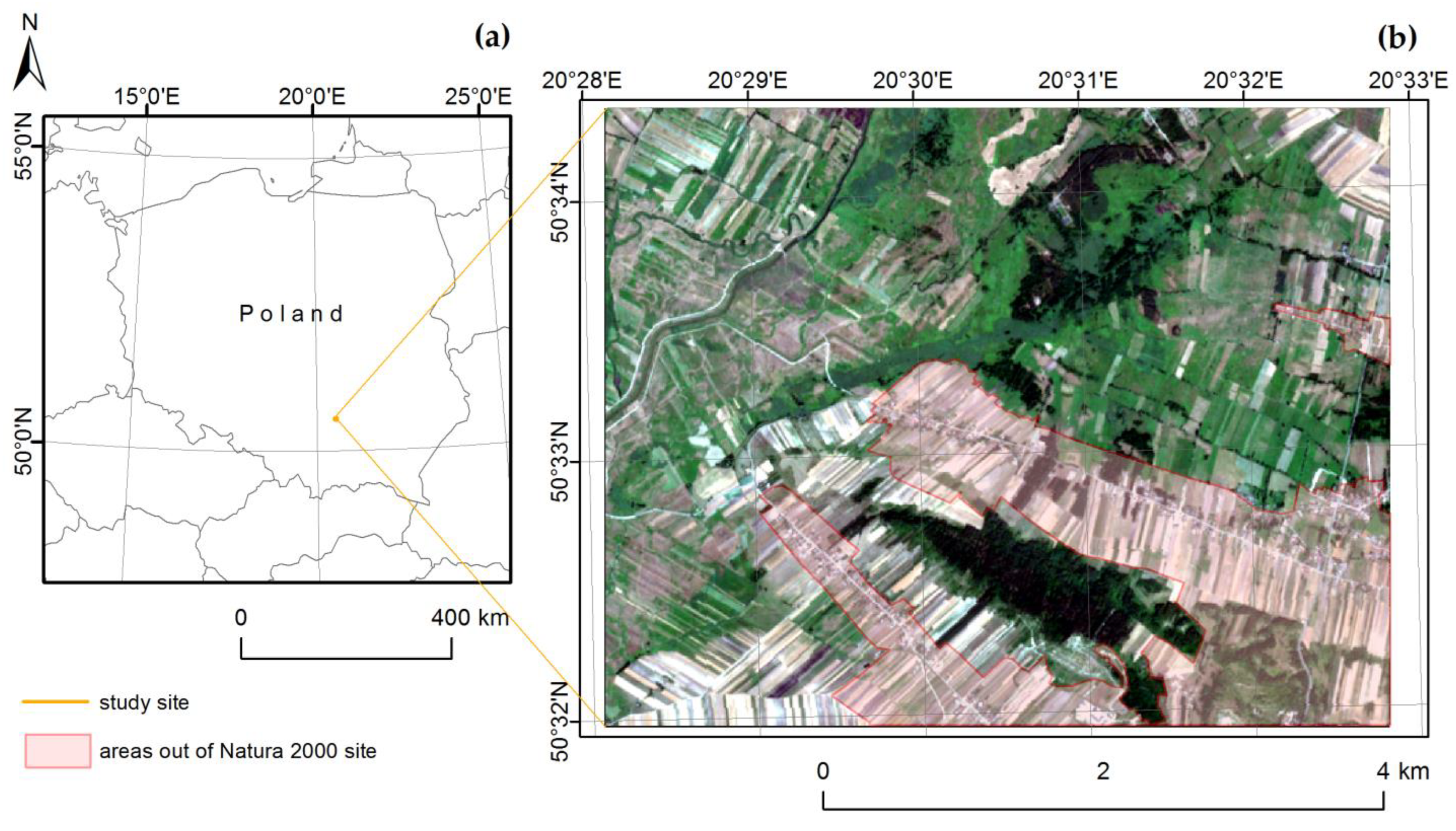
2.1. Study Site

The study area (2465 ha) is located in southern Poland. The “Ostoja Nidziańska” Natura 2000 site (code PLH260003) covers about 1894 ha, and the rest is covered mainly by built-up areas and agricultural land (about 571 ha; Figure 1).
Three grassland Natura 2000 habitats occur in this area: semi-natural dry grasslands and scrubland facies on calcareous substrates (Festuco-Brometalia, 6210 code); Molinia meadows on calcareous, peaty, or clay silt-laden soils (Molinion caeruleae, 6410 code); and lowland hay meadows (Alopecurus pratensis, Sanguisorba officinalis, 6510 code). A detailed description of them is provided in another study [7].

2.2. Ground Truth Data

The reference data came from the Habitats Airborne Remote Sensing (HabitARS) project, devoted to the use of the multisensor airborne platform to identify Natura 2000 habitats [28]. We collected the data for this study from three campaigns on 18 May, 30 July, and 27 September 2017. Measurements were performed using the Global Navigation Satellite System (GNSS) Spectra Precision GPS MobileMapper 120 receiver (Spectra Geospatial, Westminster, CA, USA). It covered three habitats and a “background” class including other non-forest vegetation communities. Detailed reference data collection for each field campaign in this area was described by the authors of another study [7]. However, because field data were initially collected for use with 1-m airborne data pixels (circle with a 3-m radius, inside the patch of the habitat), we adjusted them to the spatial resolution of Sentinel-2. In order to select only polygons that fit into the Sentinel-2 pixel grid, we visually assessed all reference data in terms of the placement of pixels (to avoid the use of mixed signals) and shadow occurrences (we excluded shadowed polygons from any date). Visual interpretation was supported with the use of 10 cm resolution aerial imagery collected synchronously with the collection of field data on 18 May, 30 July, and 27 September. Due to the fact that, apart from habitats and other communities, a substantial part of the area is covered with forests, we created an additional background class in the legend (due to small areas covered with buildings or water, we omitted these classes in the classification, assuming the possibility of imposing a vector layer presenting them from the national land cover database). We created the polygons of forests based on visual interpretations of image data. We list the number of polygons selected for each habitat and background class in Table 1.

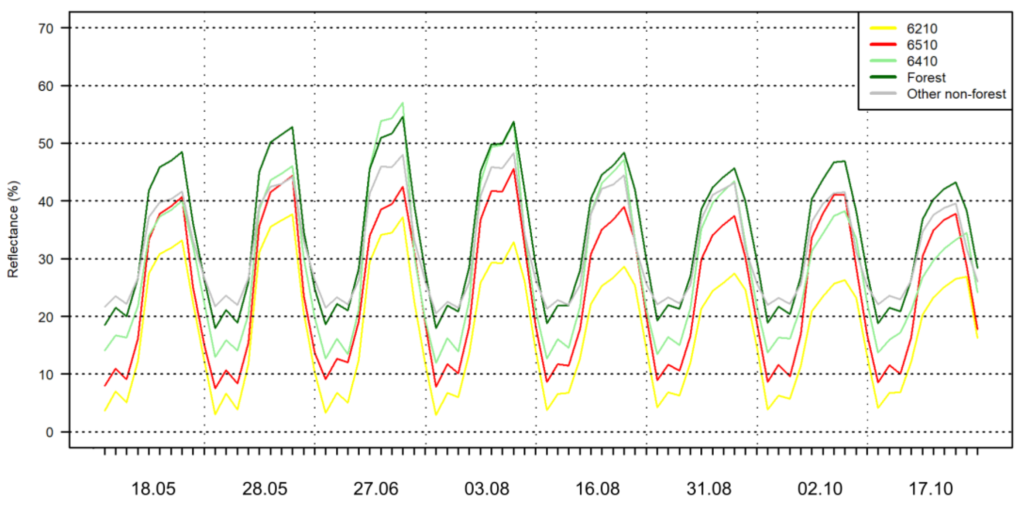
2.3. Sentinel-2 Images

We acquired Sentinel-2 scene tiles from the Copernicus Open Access Hub for the study area for the year 2017. The assumption was to use all cloudless data presenting seasonal changes for growing vegetation, which resulted in the collection of eight tiles. We present the exact dates and specific satellites (Sentinel-2A or B) in Table 2. Some vegetation studies have presented time series analyses for a whole year, including winter images [23,24,25]; however, at this latitude, the position of the sun as well as snow cover for these months affects the reflectance. Therefore, we did not apply it, and we only took the period of vegetation growth into account. As the researched habitats are semi-natural, they are mown (one or two times per year, between June and September), and we treated this feature as their specificity during the growing season. The actual mowing time of each patch varied because the studied grasslands belong to different owners.
Level-2A Bottom-Of-Atmosphere (BOA) reflectance products were available for most cases, and we only processed two downloaded images into Level-1C Top-Of-Atmosphere (TOA) products. Hence, atmospheric correction was necessary. We accomplished this using the Sentinel Application Platform (SNAP, Brockmann Consult, Skywatch, Sensar, and C-S) with the Sen2cor processor plugin [40]. Next, we removed three atmospheric bands (B1, B9, and B10) from the datasets, and we resampled the remaining 20-m bands to 10 m using the geometric operations ‘resampling’ tool in SNAP. We stacked all images into one dataset according to band order and time. We show the spectro-temporal patterns of habitats and backgrounds in Figure 2 (presenting data as a continuum across the temporal domain is motivated by the desire to exploit both the temporal and spectral domains simultaneously).

2.4. Classification and Accuracy Assessment
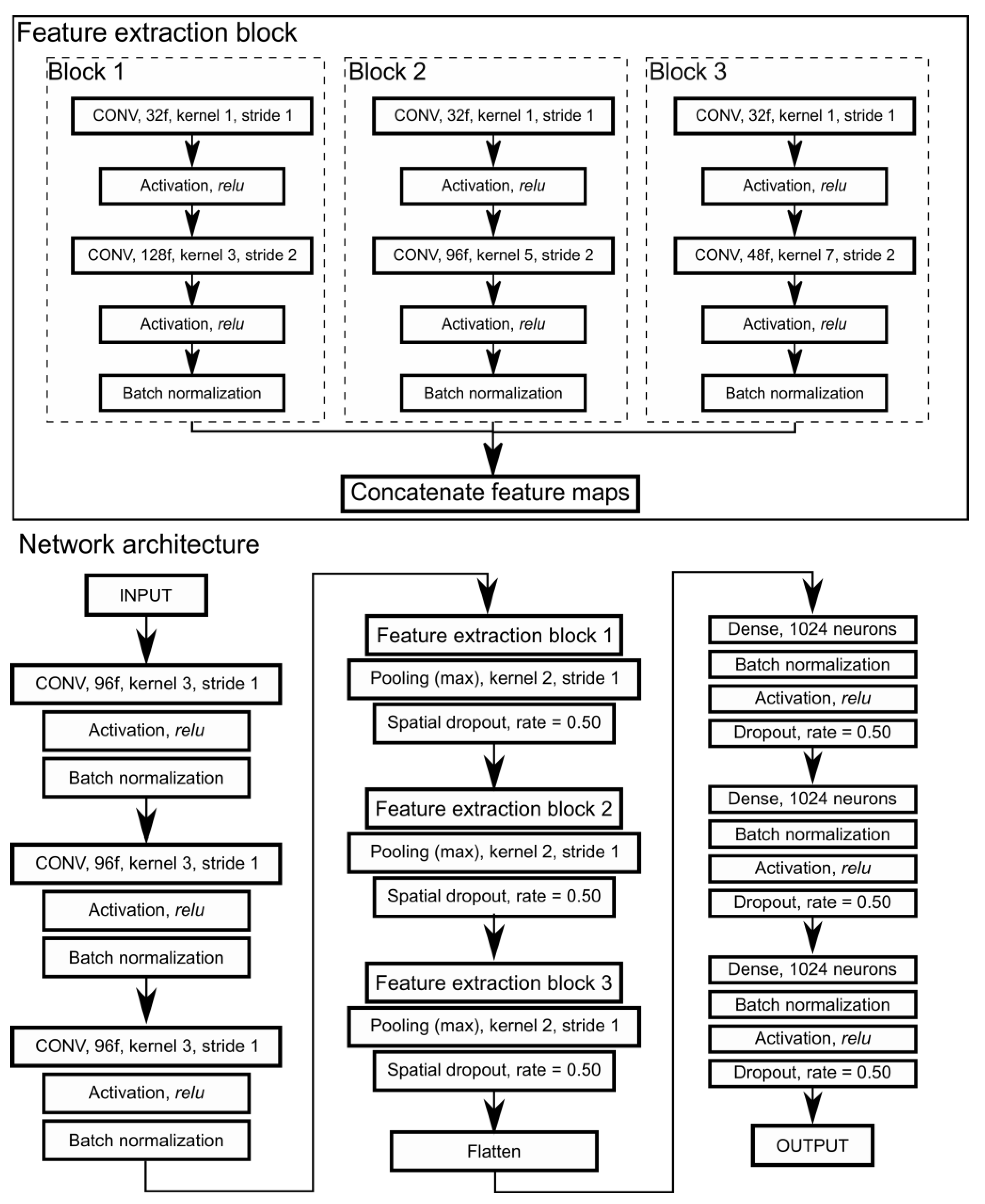
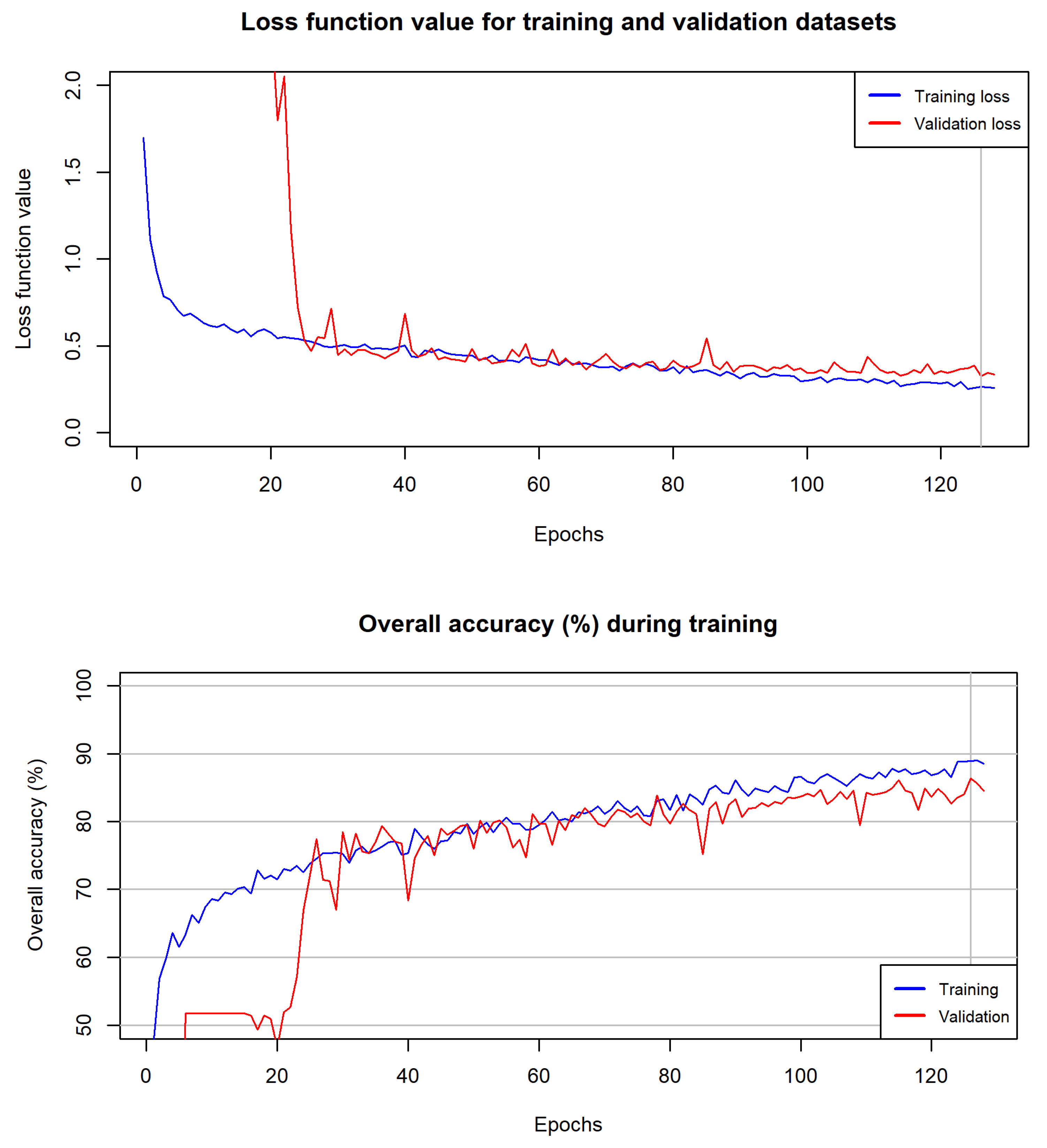
We classified the multitemporal spectral data into five classes (three habitats and two background classes) using three classification methods: Convolutional Neural Networks (CNNs), Random Forest (RF), and Support Vector Machine (SVM) (see next subsections) using the R environment [41] and a pixel-based approach. Moreover, the interactions between vector and raster data used the raster [42], rgdal [43], caret [44], and foreach [45] libraries. The hardware environment for the classifications was as follows: AMD Ryzen 2700x processor, NVIDIA GeForce GTX 1080 Ti graphics card, 16 GB of DDR 4 RAM@2933 mHz frequency, and we performed the calculations on the Samsung SSD 870QVO disc.
In order to objectively compare the tested algorithms, we used the iterative accuracy assessment technique [46]. The whole procedure repeats the algorithm training and validation process multiple times in order to reduce the influence of the training and validation datasets on the results. Typically, reference data are split into training and validation datasets either arbitrarily or randomly. Most often, this process happens only once; thus, the usefulness of randomized sampling is diminished. The iterative accuracy assessment technique splits reference data into training and validation sets 100 times using stratified random sampling. The training dataset contains 63.2% of the samples for each class, and the remaining samples are moved to the validation dataset (Table 3). Upon each iteration, each algorithm is trained using the same training dataset and is then validated using the validation dataset to assess accuracy [47]. To assess the accuracy of the obtained results, we determined the F1 accuracy for each class [48], as well as the overall accuracy (OA) for whole classified datasets [49]. We generated the final maps for each classifier using the trained model that achieved the highest mean F1 accuracy for all classes obtained from each classification.

2.4.1. CNNs

In order to simulate artificial neural networks, we used the tensorflow [50] and keras [51] libraries. We adapted the artificial neural network to use one-dimensional vectors symbolizing a time series, with the following shape: [number of samples; number of bands, 1]. We developed the CNN architecture by performing a series of experiments, and each used the same data but different architecture. We selected the most promising architecture for further work. Regarding the applied CNN architecture, the first input data was fed into three consecutive convolution layers with 96 filters each (Figure 3). The resulting data were fed into three feature extraction blocks, and each was followed by a pooling and spatial dropout layer. Lastly, the transformed data was fed into a deep neural network with three layers, each consisting of 1024 neurons, 1 normalization layer, and dropout layers. The feature extraction block is heavily inspired by Inception architecture [52], which, in principle, tries to extract both high-resolution and low-resolution patterns from the input.

2.4.2. RF

We selected the main RF parameters such as mtry, indicating the number of features selected for the best data split, and ntree, indicating the number of decision trees, based on tuning with the use of the tuneRF tool from the randomForest library, which we also used to perform the whole procedure [53]. The TuneRF procedure was controlled by parameter stepFactor equal to 1.2, starting mtry of 30 and minimum improvement over previous models was set to 0.001.

2.4.3. SVM

We performed classification with SVM using the e1071 package [54]. We performed the selection of the kernel function and training using the ‘tune.svm’ function. The following combinations of parameter C (cost) and gamma were tested: C from 10 to 1000 by 10; and gamma from 0.1 to 1 with a step of 0.1. Additionally linear, radial, polynomial, and sigmoid kernel functions were tested.

3. Results

3.1. Selected Parameters for Classifiers

For CNNs, the developed model was from the 126th epoch. The training loss function value was 0.27, and the validation loss function value was 0.32 (Figure 4).
The selected parameter values for the RF method were as follows: ntree, 500; and mtry, 36. The literature confirms that having the number of trees equal to 500 stabilizes the errors before this number is achieved [55].
For SVM, we chose RBF, and from parameter tuning, we determined that the best configuration was C equal to 1000 and gamma equal to 0.1.

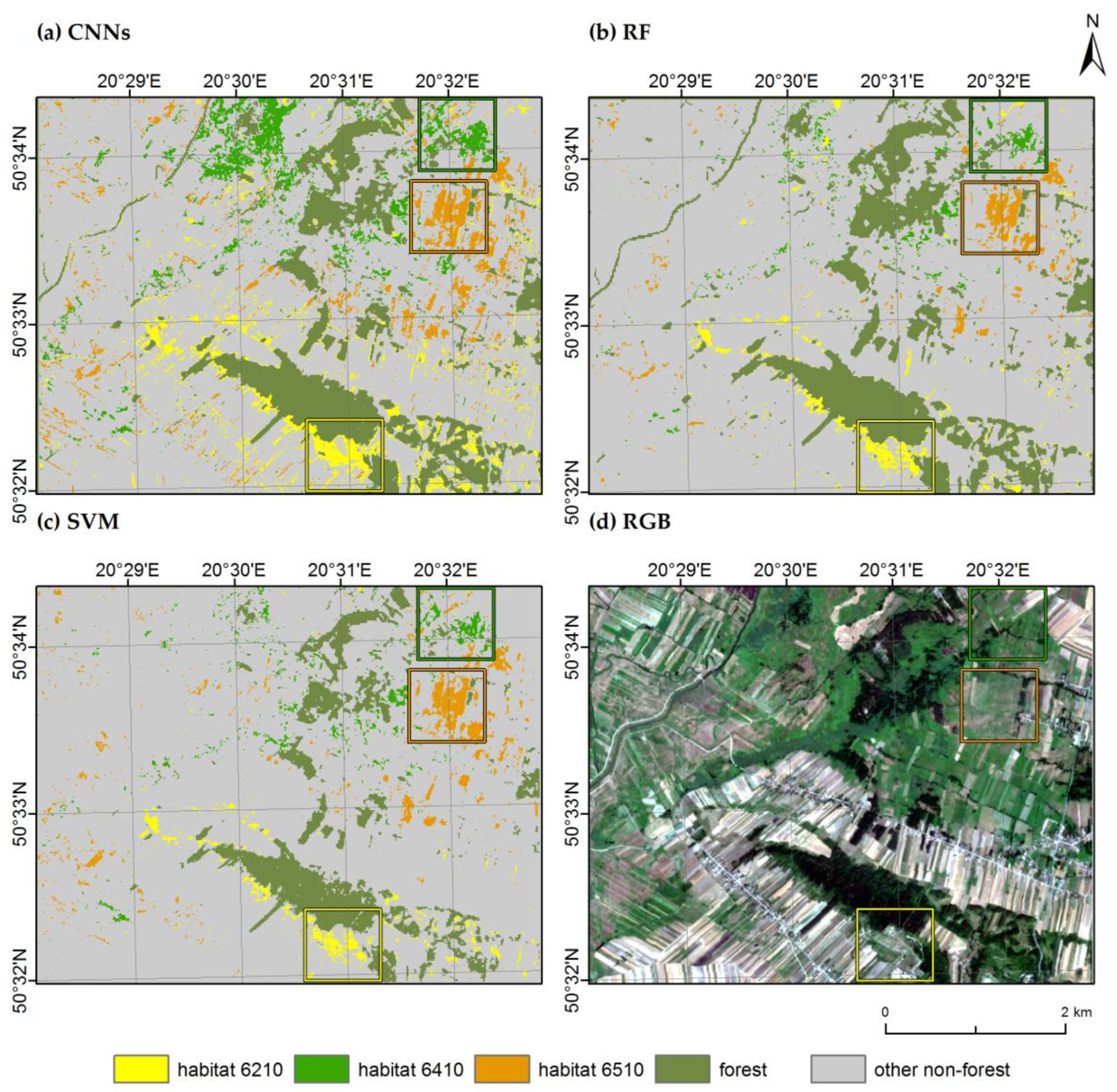
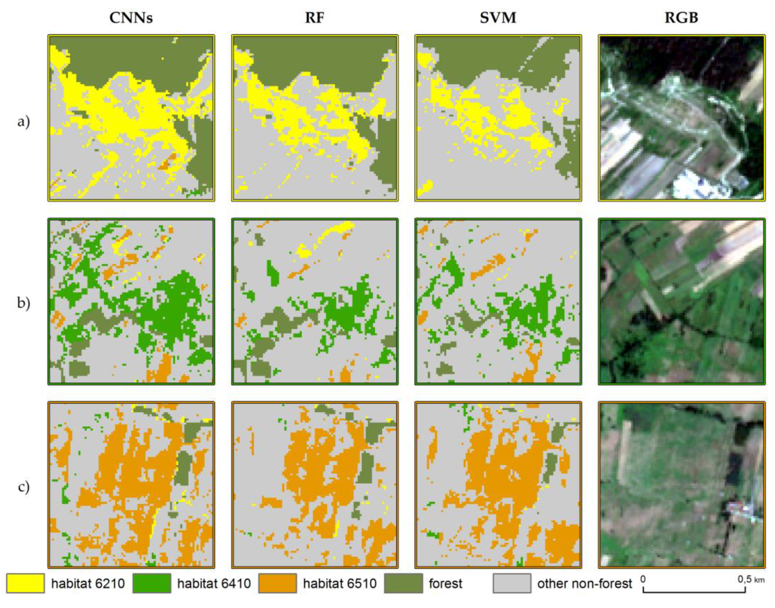
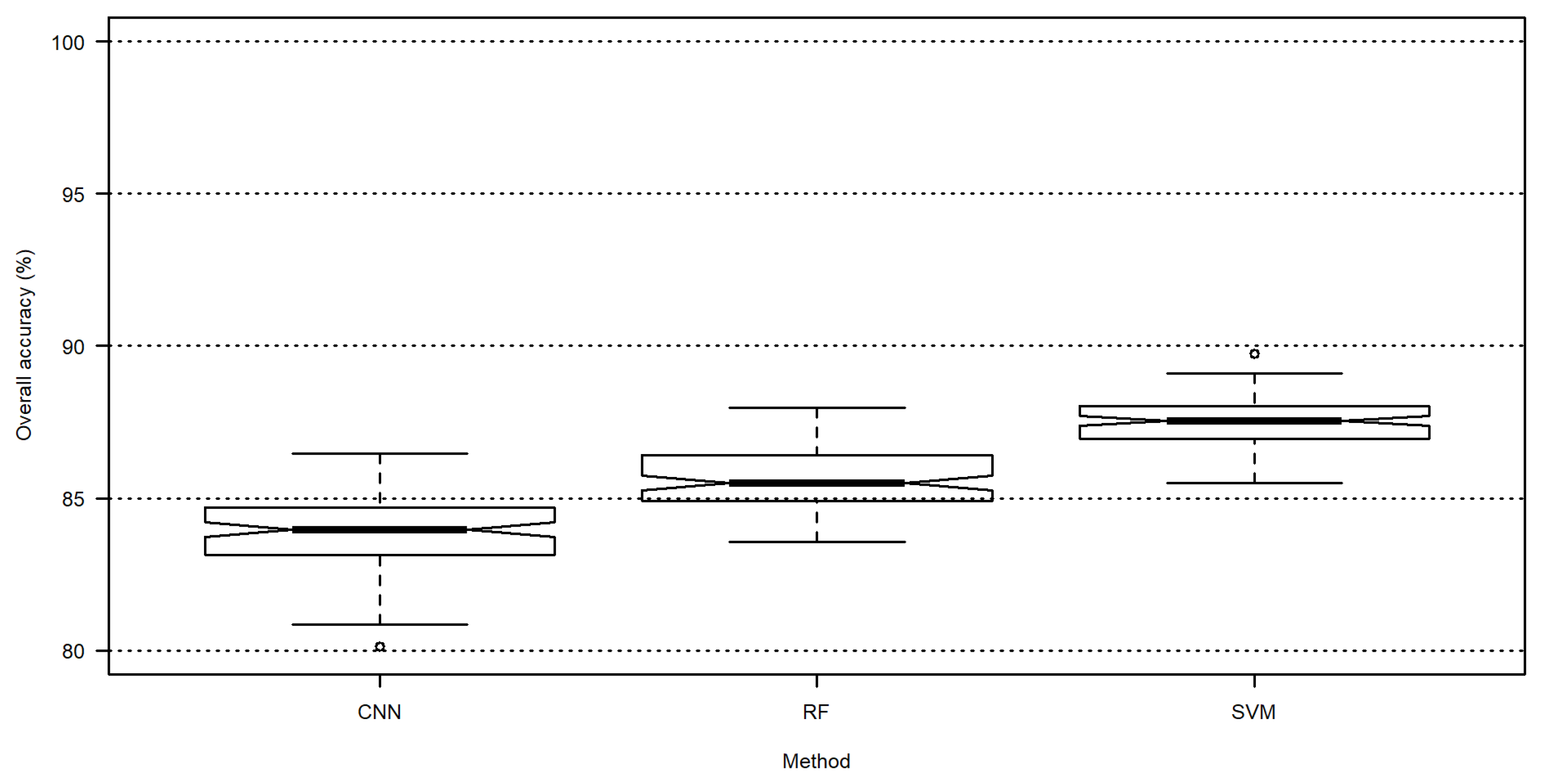
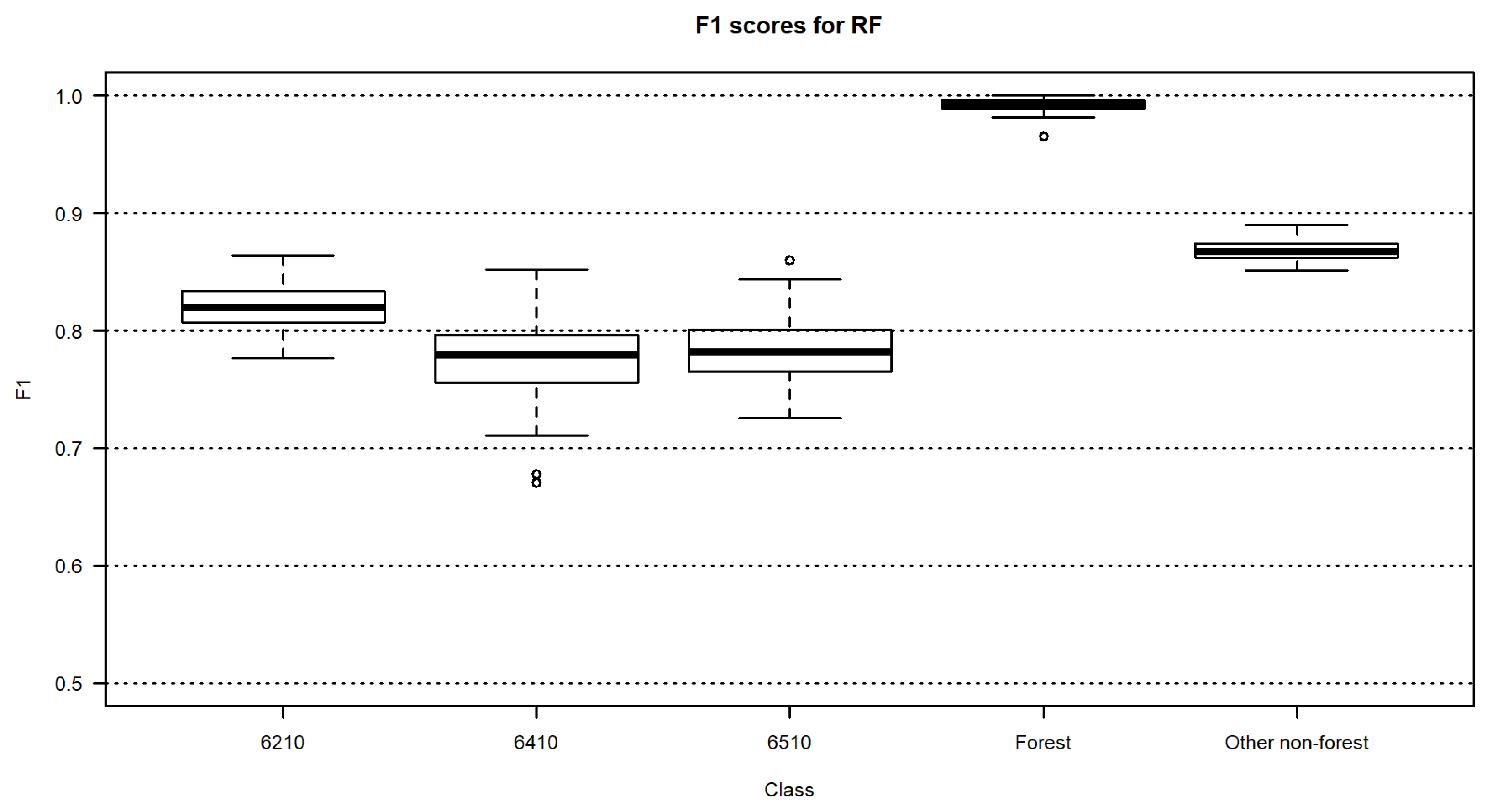
3.2. Habitat Maps and Accuracies

As a result of each classification, we obtained maps of the distribution of the five classes (Figure 5a–c and Figure 6a–c). Their qualitative assessment, in general, showed a similar distribution of habitats and background classes. By analyzing the algorithms’ performances, we observed that the map produced with CNNs appeared to be more detailed than that of RF and SVM, and some habitats were overestimated (in particular, habitat 6410 in the north part of the area where the floodplain actually is; Figure 5a). In addition, a slight mixing of the other non-forest background classes with habitat classes was noticeable (the habitats themselves did not mix with each other).
More specifically, habitat 6210, occurring on the slopes, was mainly classified along the hill covered with forests (Figure 6a). On the resulting maps from CNNs and RF, it is slightly overestimated, which also occurred in other parts of the image (e.g., Figure 6b,c), where no conditions were conducive to their occurrence. Many smaller patches of habitat 6410 along the roads were also overestimated on the CNN map. Habitat 6510 was quite similarly classified on three maps; however, most pixels classified as habitats were on the CNN map. The SVM maps, in all cases, seemed to overestimate habitats the least; however, forests could sometimes be underestimated (trees along the roads; Figure 6a–c). Larger parts of the area were covered by the class of other non-forests, which we used to determine the greatest amount of reference data to be able to distinguish them as much as possible from habitats.
In general, using the proposed methods, we were able to obtain high OAs (median values from the 100-fold accuracy assessment were higher than 0.84; Figure 7). Comparing the algorithms’ performances, the best OAs were reached for SVM (median value around 0.88), and the worst were for CNNs (0.84). As can be noticed, differences between median values did not exceed 4 percentage points (p.p.). Moreover, the minimum and maximum noted values were rather small (5 p.p. and 3 p.p., respectively). The values for RF and SVM were more stable, giving a difference between the minimum and maximum values of 4 p.p., but for CNNs, such a difference could be considered negligible.
We obtained more diverse results for individual classes, and we focused more on F1 accuracy for each habitat and background class. Boxplots with bolded median values below (Figure 8, Figure 9 and Figure 10) present the accuracies obtained for each classifier separately.
With CNNs, the median F1 accuracy for habitat 6210 was equal to 0.842, and for 6410 and 6510, the values were 0.758 and 0.768, respectively. For habitat 6410, we obtained the widest range of accuracy values. The median F1 was equal to 0.839 for other non-forest vegetation and 0.993 for forests.
With RF, the findings were similar; however, the median value of F1 was lower for habitat 6210 (0.819). For both 6410 and 6510, it was around 0.78, and we found the most varied values for 6410. Apart from the forest class (0.993), we recorded the highest median in this case for the other non-forest background class (0.867).
The habitat 6210 class achieved the highest possible accuracy with SVM (0.853), and a similar value was achieved by the 6510 class. For this classifier, apart from forests, the other non-forest class was classified the second-best, and we obtained the slowest value for the 6410 class (0.804). Compared with previously described results, forests reached a lower median F1 value (0.962), and the value range was wider.
In general, the trend was the same for all results obtained with the three classifiers. Among the three grassland habitats, we found the highest 100-fold F1 accuracy medians for habitat 6210, we found the lowest for habitat 6410, and they were very similar for habitat 6510. Both background classes (forest and other non-forest) had better discrimination, and the ranges of their values were more stable (particularly for the forest class) for each classification.
SVM allowed us to achieve the best results for the majority of cases, i.e., all habitats and other non-forest vegetation (F1 median values in the range of 0.844–0.962; Table 4). We noted the highest difference between median F1 values for the 6510 class, which, for SVM, was 8 p.p. more than that of CNNs. We found the most stable results between different algorithms for the 6210 and forest classes (3 p.p. between RF and SVM). For habitat 6410 and the other non-forest class, the difference between the lowest (CNNs) and the highest (SVM) was equal to 3 p.p.

4. Discussion

Research with Sentinel-2 data and their high temporal resolution, capable of supporting the retrieval of temporal features, was suggested by the authors of previous studies regarding habitat classification [3]. In studies of wetland habitats, multitemporal Sentinel-2 data led to obtaining higher accuracies than those for single-date collection data [22]. Moreover, Fenske et al. [13] suggested a direct comparison between hyperspectral and multitemporal data for the use of the same classification approach. It was further developed for different Natura 2000 habitats, including grasslands [10]. Our work can also be compared with results previously obtained from the same research area [7] using multitemporal hyperspectral data fused with topographic indices and an RF classifier (Table 5).
The combination of different terms of data acquisition leads to obtaining better accuracy than that with the use of single-date collection data [7]. Hence, in this study, we decided to use all possible images to capture phenology variations across the whole vegetative period. In general, the potential of multitemporal Sentinel-2 data in the classification of grassland Natura 2000 habitats, as presented in this article, is confirmed by its consistency within a previous study (especially for habitats 6210 and 6410) and its high accuracies for all classes (median F1 value greater than 0.70 in each case). For habitat 6510, with hyperspectral data, the F1 accuracies were worse than those obtained with multispectral data (the maximum obtained median value was approximately 0.70). This may be influenced by the co-occurrence of species forming it and species of the other non-forest vegetation class. In the case of a 1-m pixel, more possibilities are given to notice the transition zone between habitats and the background, and this information is generalized in a pixel of 10 m. Moreover, notably, we modified the reference data to the pixel size of Sentinel-2, so a direct comparison of the obtained accuracies should be treated carefully. However, by analyzing both spectral and temporal dimensions, we can conclude that, for these habitats, the discrimination of dense time series with even only the spectral index can be better than the use of several acquisitions with many spectral bands. In this case, the choice of bands is the key to performing the study as accurately as possible (e.g., Jarocińska et al. [10] found that the most useful spectral ranges for different Natura 2000 habitat discrimination are as follows: in VNIR, 0.416–0.442 µm and 0.502–0.522 µm; and in SWIR, 1.117–1.165 µm and 1.290–1.361 µm). From an operational point of view, utilizing access to Sentinel-2 data is a promising solution to monitoring Natura 2000 habitats.
In the work presented here, we did not utilize any additional data sources, e.g., Shuttle Radar Topography Mission (SRTM) and its derivatives, which could have potentially improved the accuracies. Such improvements can be seen in the work of Tarantino et al. [24], who also utilized the Sentinel-2 time series for mapping habitat 6210 in Italy. In research on hyperspectral data [7], LiDAR-based topographic indices were incorporated, which was important for improving the results of mapping habitats 6210 and 6410; however, the differences in accuracies obtained with and without them were negligible (Table 5). Hence, in this study, we wanted to explore the spectral-temporal dimension, and our assumed approach was also based on the conclusions of another study [23], which proved that phenological variations in the Sentinel-2 time series are more important than the topographic and lithological variables in the classification of forest habitats.
Habitats 6410 and 6510, analyzed in different sites in Poland, were the object of study in other research [10], where, with multispectral Sentinel-2 data, discrimination from background classes with Linear Discriminant Analysis (LDA) was assessed as lower than that of heaths and mires habitats (codes 4030 and 7140, respectively). However, the authors also underlined that the results were strictly dependent on the site and background classes. This also applies to our study because, in general, areas with high biodiversity are characterized by the fact that they are unique, and in each place, the background and combination of species are slightly different. Building knowledge in this case is based on the analysis of specific case studies and then checking the possibilities of using this knowledge in other research.
The application of iterative accuracy assessments or other alternatives allows one to investigate not only raw accuracy measures as a single number, but it can also allow one to see the distribution of obtained accuracy measures per class. This can greatly help with understanding how given classes are classified and allows for straightforward comparisons to be made between results coming from different algorithms or models built using differing sets of parameters. This approach was also presented in work on the Ostoja Nidziańska area [7], and the ranges of minimum and maximum values of F1 accuracies for habitat classes were comparable to those in this article (less than 15 p.p. for each habitat class). This is confirmed by the preparation of representative reference data for classification. When the number of samples is insufficient, or when data are less representative of a class, value distributions can be wide, such as above 30 p.p. for 3 out of 22 classes of the mappings of plant communities [56].
CNNs can utilize both spectral and spatial data in order to classify images. In this work, we refrained from using spatial data due to a low spatial resolution and the relative congestion of reference plots, considering the spatial resolution of underlying raster data. Utilizing the spatial domain would necessitate the inclusion of additional neighboring pixels, covered by a window of a given size (in pixels) and centered for each reference pixel. In summary, we are not able to provide a sufficiently large reference dataset, which would not result in an excessive number of samples containing partially the same data (spatial autocorrelation, [57]). If one considers utilizing both the spectral and spatial domains, more care and planning must be used while collecting reference data, with the critical parameter being sufficient spacing between them. Such a patch-wise approach tessellating training data in different square patches was presented in another work [25]. One of the habitats classified in that work in Italy was also in Poland (6210). The accuracy of F1 in the work for this habitat ranged from 62 to 100%, and notably, the highest was obtained for the largest patch (6 × 6), for which the smallest amount of training data was used. However, as mentioned in other research [23], the same species-forming habitats can have different behaviors in terms of phenology in a different geographic bioclimatic context, so we should not compare these results directly. In the future, reference data can be collected in the manner mentioned above, and a spatial approach can also be used in CNN classification.
In our work, we wanted to focus on the spectro-temporal dimension of Sentinel-2 data due to the comparison of different classifiers. The applied CNNs had approximately 4,200,000 trainable parameters, with about 2,500,000 used in the deep network part. Therefore, the training process lasted much longer than that for the RF and SVM methods. However, the results were comparable. The largest difference in the OA median was 4 p.p. in favor of SVM vs. CNNs. However, in the literature, CNNs have shown performance improvements over RF and SVM, e.g., utilizing the spatial dimension [58], based on UAV hyperspectral analysis [59], or in plastic greenhouse mapping based on dual-temporal Sentinel-2 data [60]. Considering the comparison between SVM and RF, SVM was better, with many more features [20,32], and this can be confirmed by our results, in which we incorporated 80 spectro-temporal features into our classifications. Some studies have reported that SVM performs better with imbalanced or small sample sets [29,56,61], making this algorithm unique in situations in which creating a balanced/large data set is not possible. In fact, due to operational issues such as speed and reliability, RF is most commonly used in habitat mapping [3,7,12,62]. Although we obtained a slightly lower habitat accuracy for CNNs, a conclusion should not be made in this regard. Its big advantage is that it extracts information during the classification itself, and with a larger number of variables (more terms of data acquisition), it is not as vulnerable to the curse of dimensionality that occurs sooner with a large number of variables in SVM or RF. Convolutional networks offer opportunities for modification on an ongoing basis (e.g., the number of features and the depth of the network), which we plan to explore more in future studies on habitats.

5. Conclusions

In this work, including the classification of Natura 2000 grassland habitats using Sentinel-2 spectro-temporal data, we showed that the algorithms used were sufficient for creating accurate maps of habitats. Notably, all the algorithms were able to properly classify habitat 6210, and we obtained slightly lower accuracies for habitats 6410 and 6510, which may have been caused by the spectral similarity of forming species with the other non-forest vegetation class. In general, SVM appeared to be better than RF and CNNs for mapping grassland habitats using mutitemporal Sentinel-2 datasets (OA and F1 for three habitats were the highest with SVM); however, the differences were very small. Researchers using CNNs should consider using a spectro-temporal dataset with a spatial domain in order to achieve better results. CNNs incorporate the spatial domain into their solutions in ways that are unavailable to other, more conventional algorithms, such as RF and SVM. Nevertheless, the spectral dimension can be analyzed even more deeply, and it can be considered for use in multiple endmember spectral mixture analysis (MESMA, [63]) to determine the likely composition of each image in a multitemporal dataset.
Although the trained models were not useful for creating new maps on the fly, the presented method is transferable to other areas. Another weakness is that it cannot be generalized enough to use any combination of spectro-temporal data. However, our presented workflow and choice of algorithms can be useful for other studies on grassland habitats. Additionally, regardless of the algorithm used, for the purpose of monitoring the work of grassland Natura 2000 habitats, Sentinel-2 is valuable and promising because it provides cost reductions and the possibility of quickly acquiring new data for updating existing maps.

Author Contributions

Conceptualization, A.M.-O., E.R. and A.O.; methodology, A.M.-O. and E.R.; software, E.R. and A.M.-O.; validation, A.O., E.R. and A.M.-O.; formal analysis, A.M.-O.; investigation, A.M.-O., E.R. and A.O.; resources, A.O., A.M.-O. and D.K.; data curation, A.O.; writing—original draft preparation, A.M.-O.; writing—review and editing, all; visualization, E.R., A.O. and A.M.-O.; supervision, A.M.-O. and D.K. All authors have read and agreed to the published version of the manuscript.

Funding

Field data collection were from the project funded by the Polish National Centre for Research and Development (NCBR) under the programme “Natural Environment, Agriculture and Forestry” BIOSTRATEG II.: The innovative approach supporting monitoring of non-forest Natura 2000 habitats, using remote sensing methods (HabitARS), grant number: DZP/BIOSTRATEG-II/390/2015.

Institutional Review Board Statement

Not applicable.

Informed Consent Statement

Not applicable.

Data Availability Statement

The Sentinel-2 data can be accessed at (https://scihub.copernicus.eu/, accessed on 20 December 2022). Ground truth data from HabitARS project are not publicly available.

Acknowledgments

Authors would like to thank to Beata Babczyńska-Sendek, Agnieszka Błońska, Agnieszka Kompała-Bąba, Teresa Nowak, Barbara Tokarska-Guzik and Beata Węgrzynek for ground truth data acquisition, and to Dominik Żmuda for consulting on habitats classification in this area. The authors also express their gratitude to three anonymous reviewers who contributed to the improvement of the manuscript through their experience.

Conflicts of Interest

The authors declare no conflict of interest.

References

  1. European Comission Council. European Comission Council Directive 92/43/EEC of 21 May 1992 on the conservation of natural habitats and of wild fauna and flora (OJ L 206 22.07.1992 p. 7). Doc. Eur. Community Environ. Law 2010, 206, 568–583. [Google Scholar] [CrossRef]
  2. Habel, J.C.; Dengler, J.; Janišová, M.; Török, P.; Wellstein, C.; Wiezik, M. European grassland ecosystems: Threatened hotspots of biodiversity. Biodivers. Conserv. 2013, 22, 2131–2138. [Google Scholar] [CrossRef] [Green Version]
  3. Buck, O.; Millán, V.E.G.; Klink, A.; Pakzad, K. Using information layers for mapping grassland habitat distribution at local to regional scales. Int. J. Appl. Earth Obs. Geoinf. 2015, 37, 83–89. [Google Scholar] [CrossRef]
  4. Schuster, C.; Schmidt, T.; Conrad, C.; Kleinschmit, B.; Förster, M. Grassland habitat mapping by intra-annual time series analysis -Comparison of RapidEye and TerraSAR-X satellite data. Int. J. Appl. Earth Obs. Geoinf. 2015, 34, 25–34. [Google Scholar] [CrossRef]
  5. Feilhauer, H.; Thonfeld, F.; Faude, U.; He, K.S.; Rocchini, D.; Schmidtlein, S. Assessing floristic composition with multispectral sensors-A comparison based: On monotemporal and multiseasonal field spectra. Int. J. Appl. Earth Obs. Geoinf. 2012, 21, 218–229. [Google Scholar] [CrossRef]
  6. Große-Stoltenberg, A.; Hellmann, C.; Werner, C.; Oldeland, J.; Thiele, J. Evaluation of continuous VNIR-SWIR spectra versus narrowband hyperspectral indices to discriminate the invasive Acacia longifolia within a mediterranean dune ecosystem. Remote Sens. 2016, 8, 334. [Google Scholar] [CrossRef] [Green Version]
  7. Marcinkowska-Ochtyra, A.; Gryguc, K.; Ochtyra, A.; Kopeć, D.; Jarocińska, A.; Sławik, Ł. Multitemporal Hyperspectral Data Fusion with Topographic Indices—Improving Classification of Natura 2000 Grassland Habitats. Remote Sens. 2019, 11, 2264. [Google Scholar] [CrossRef] [Green Version]
  8. Pérez-Carabaza, S.; Boydell, O.; O’Connell, J. Habitat classification using convolutional neural networks and multitemporal multispectral aerial imagery. J. Appl. Remote Sens. 2021, 15, 042406. [Google Scholar] [CrossRef]
  9. Demarchi, L.; Kania, A.; Ciezkowski, W.; Piórkowski, H.; Oświecimska-Piasko, Z.; Chormański, J. Recursive feature elimination and random forest classification of natura 2000 grasslands in lowland river valleys of poland based on airborne hyperspectral and LiDAR data fusion. Remote Sens. 2020, 12, 1824. [Google Scholar] [CrossRef]
  10. Jarocińska, A.; Kopeć, D.; Kycko, M.; Piórkowski, H.; Błońska, A. Hyperspectral vs. Multispectral data: Comparison of the spectral differentiation capabilities of Natura 2000 non-forest habitats. ISPRS J. Photogramm. Remote Sens. 2022, 184, 148–164. [Google Scholar] [CrossRef]
  11. Stenzel, S.; Feilhauer, H.; Mack, B.; Metz, A.; Schmidtlein, S. Remote sensing of scattered natura 2000 habitats using a one-class classifier. Int. J. Appl. Earth Obs. Geoinf. 2014, 33, 211–217. [Google Scholar] [CrossRef]
  12. Feilhauer, H.; Dahlke, C.; Doktor, D.; Lausch, A.; Schmidtlein, S.; Schulz, G.; Stenzel, S. Mapping the local variability of Natura 2000 habitats with remote sensing. Appl. Veg. Sci. 2014, 17, 765–779. [Google Scholar] [CrossRef]
  13. Fenske, K.; Feilhauer, H.; Förster, M.; Stellmes, M.; Waske, B. Hierarchical classification with subsequent aggregation of heathland habitats using an intra-annual RapidEye time-series. Int. J. Appl. Earth Obs. Geoinf. 2020, 87, 102036. [Google Scholar] [CrossRef]
  14. Sittaro, F.; Hutengs, C.; Semella, S.; Vohland, M. A Machine Learning Framework for the Classification of Natura 2000 Habitat Types at Large Spatial Scales Using MODIS Surface Reflectance Data. Remote Sens. 2022, 14, 823. [Google Scholar] [CrossRef]
  15. Grabska, E.; Hostert, P.; Pflugmacher, D.; Ostapowicz, K. Forest stand species mapping using the sentinel-2 time series. Remote Sens. 2019, 11, 1197. [Google Scholar] [CrossRef] [Green Version]
  16. Hościło, A.; Lewandowska, A. Mapping Forest Type and Tree Species on a Regional Scale Using Multi-Temporal Sentinel-2 Data. Remote Sens. 2019, 11, 929. [Google Scholar] [CrossRef] [Green Version]
  17. Pesaresi, S.; Mancini, A.; Quattrini, G.; Casavecchia, S. Mapping mediterranean forest plant associations and habitats with functional principal component analysis using Landsat 8 NDVI time series. Remote Sens. 2020, 12, 1132. [Google Scholar] [CrossRef] [Green Version]
  18. Praticò, S.; Solano, F.; Di Fazio, S.; Modica, G. Machine learning classification of mediterranean forest habitats in google earth engine based on seasonal sentinel-2 time-series and input image composition optimisation. Remote Sens. 2021, 13, 586. [Google Scholar] [CrossRef]
  19. Immitzer, M.; Neuwirth, M.; Böck, S.; Brenner, H.; Vuolo, F.; Atzberger, C. Optimal Input Features for Tree Species Classification in Central Europe Based on Multi-Temporal Sentinel-2 Data. Remote Sens. 2019, 11, 2599. [Google Scholar] [CrossRef] [Green Version]
  20. Rapinel, S.; Mony, C.; Lecoq, L.; Clément, B.; Thomas, A.; Hubert-Moy, L. Evaluation of Sentinel-2 time-series for mapping floodplain grassland plant communities. Remote Sens. Environ. 2019, 223, 115–129. [Google Scholar] [CrossRef]
  21. Wakulinśka, M.; Marcinkowska-Ochtyra, A. Multi-temporal sentinel-2 data in classification of mountain vegetation. Remote Sens. 2020, 12, 2696. [Google Scholar] [CrossRef]
  22. Le Dez, M.; Robin, M.; Launeau, P. Contribution of Sentinel-2 satellite images for habitat mapping of the Natura 2000 site ‘Estuaire de la Loire’ (France). Remote Sens. Appl. Soc. Environ. 2021, 24, 100637. [Google Scholar] [CrossRef]
  23. Pesaresi, S.; Mancini, A.; Quattrini, G.; Casavecchia, S. Functional Analysis for Habitat Mapping in a Special Area of Conservation Using Sentinel-2 Time-Series Data. Remote Sens. 2022, 14, 1179. [Google Scholar] [CrossRef]
  24. Tarantino, C.; Forte, L.; Blonda, P.; Vicario, S.; Tomaselli, V.; Beierkuhnlein, C.; Adamo, M. Intra-annual sentinel-2 time-series supporting grassland habitat discrimination. Remote Sens. 2021, 13, 277. [Google Scholar] [CrossRef]
  25. Fazzini, P.; Proia, G.D.F.; Adamo, M.; Blonda, P.; Petracchini, F.; Forte, L.; Tarantino, C. Sentinel-2 remote sensed image classification with patchwise trained convnets for grassland habitat discrimination. Remote Sens. 2021, 13, 2276. [Google Scholar] [CrossRef]
  26. Breiman, L. Random Forests LEO. Mach. Learn. 2001, 45, 5–32. [Google Scholar] [CrossRef] [Green Version]
  27. Osińska-Skotak, K.; Radecka, A.; Piórkowski, H.; Michalska-Hejduk, D.; Kopeć, D.; Tokarska-Guzik, B.; Ostrowski, W.; Kania, A.; Niedzielko, J. Mapping Succession in Non-Forest Habitats by Means of Remote Sensing: Is the Data Acquisition Time Critical for Species Discrimination? Remote Sens. 2019, 11, 2629. [Google Scholar] [CrossRef] [Green Version]
  28. Sławik, Ł.; Niedzielko, J.; Kania, A.; Piórkowski, H.; Kopeć, D. Multiple flights or single flight instrument fusion of hyperspectral and ALS data? A comparison of their performance for vegetation mapping. Remote Sens. 2019, 11, 913. [Google Scholar] [CrossRef] [Green Version]
  29. Burai, P.; Deák, B.; Valkó, O.; Tomor, T. Classification of herbaceous vegetation using airborne hyperspectral imagery. Remote Sens. 2015, 7, 2046–2066. [Google Scholar] [CrossRef] [Green Version]
  30. Sabat-Tomala, A.; Raczko, E.; Zagajewski, B. Comparison of Support Vector Machine and Random Forest Algorithms for Invasive and Expansive Species Classification Using Airborne Hyperspectral Data. Remote Sens. 2020, 12, 516. [Google Scholar] [CrossRef] [Green Version]
  31. Zagajewski, B.; Kluczek, M.; Raczko, E.; Njegovec, A.; Dabija, A.; Kycko, M. Comparison of random forest, support vector machines, and neural networks for post-disaster forest species mapping of the krkonoše/karkonosze transboundary biosphere reserve. Remote Sens. 2021, 13, 2581. [Google Scholar] [CrossRef]
  32. Sheykhmousa, M.; Mahdianpari, M.; Ghanbari, H.; Mohammadimanesh, F.; Ghamisi, P.; Homayouni, S. Support Vector Machine Versus Random Forest for Remote Sensing Image Classification: A Meta-Analysis and Systematic Review. IEEE J. Sel. Top. Appl. Earth Obs. Remote Sens. 2020, 13, 6308–6325. [Google Scholar] [CrossRef]
  33. Dabija, A.; Kluczek, M.; Zagajewski, B.; Raczko, E.; Kycko, M.; Al-Sulttani, A.H.; Tardà, A.; Pineda, L.; Corbera, J. Comparison of support vector machines and random forests for corine land cover mapping. Remote Sens. 2021, 13, 777. [Google Scholar] [CrossRef]
  34. Vapnik, V.N. An overview of statistical learning theory. IEEE Trans. Neural Netw. 1999, 10, 988–999. [Google Scholar] [CrossRef] [Green Version]
  35. LeCun, Y.; Bottou, L.; Bengio, Y.; Haffner, P. Gradient-based learning applied to document recognition. Proc. IEEE 1998, 86, 2278–2324. [Google Scholar] [CrossRef] [Green Version]
  36. Krizhevsky, A.; Sutskever, I.; Hinton, G.E. Imagenet classification with deep convolutional neural networks. In Advances in neural information. Commun. ACM 2017, 60, 84–90. [Google Scholar] [CrossRef] [Green Version]
  37. Krówczyńska, M.; Raczko, E.; Staniszewska, N.; Wilk, E. Asbestos-cement roofing identification using remote sensing and convolutional neural networks (CNNs). Remote Sens. 2020, 12, 408. [Google Scholar] [CrossRef] [Green Version]
  38. Guo, Z.; Chen, Q.; Wu, G.; Xu, Y.; Shibasaki, R.; Shao, X. Village building identification based on Ensemble Convolutional Neural Networks. Sensors 2017, 17, 2487. [Google Scholar] [CrossRef] [Green Version]
  39. GDOŚ. Available online: https://www.gov.pl/web/gdos/dostep-do-danych-geoprzestrzennych (accessed on 14 January 2023).
  40. Main-Knorn, M.; Pflug, B.; Louis, J.; Debaecker, V.; Müller-Wilm, U.; Gascon, F. Sen2Cor for Sentinel-2. Proc. SPIE 2017, 10427, 1042704. [Google Scholar]
  41. R Core Team. R: A Language and Environment for Statistical Computing; R Foundation for Statistical Computing: Vienna, Austria, 2020; Available online: https://www.R-project.org/ (accessed on 18 November 2022).
  42. Hijmans, R.J.; van Etten, J. raster: Geographic Analysis and Modeling with Raster Data. R Packag. Version 2.5-2. 2015. Available online: https://CRAN.R-project.org/package=raster (accessed on 20 November 2022).
  43. Bivand, R.; Keitt, T.; Rowlingson, B. Package ‘rgdal’—Bindings for the “Geospatial” Data Abstraction Library; 2019. Available online: http://www.tinyurl.com/h8w8n29 (accessed on 10 January 2023).
  44. Kuhn, M. Contributions from Jed Wing, Steve Weston, Andre Williams, Chris Keefer, Allan Engelhardt, Tony Cooper, Zachary Mayer, Brenton Kenkel, the R Core Team, Michael Benesty, Reynald Lescarbeau, Andrew Ziem, Luca Scrucca, Yuan Tang, Can Candan, and T. H. caret: Classification and Regression Training. R Packag. Version 6.0-79. 2018. Available online: https://www.machinelearningplus.com/machine-learning/caret-package/ (accessed on 10 January 2023).
  45. Weston, S. Getting Started with doSMP and Foreach. R Packag. Version. 2011; pp. 2–7. Available online: https://cran.r-project.org/web/packages/doMC/vignettes/gettingstartedMC.pdf (accessed on 10 January 2023).
  46. Raczko, E.; Zagajewski, B. Tree species classification of the UNESCO man and the biosphere Karkonoski National Park (Poland) using artificial neural networks and APEX hyperspectral images. Remote Sens. 2018, 10, 1111. [Google Scholar] [CrossRef] [Green Version]
  47. Ghosh, A.; Fassnacht, F.E.; Joshi, P.K.; Kochb, B. A framework for mapping tree species combining hyperspectral and LiDAR data: Role of selected classifiers and sensor across three spatial scales. Int. J. Appl. Earth Obs. Geoinf. 2014, 26, 49–63. [Google Scholar] [CrossRef]
  48. Van Rijsbergen, C.J. Information Retrieval, 2nd ed.; Butterworths: London, UK, 1979; Volume 208, pp. 374–375. [Google Scholar]
  49. Congalton, R.G. A review of assessing the accuracy of classifications of remotely sensed data. Remote Sens. Environ. 1991, 37, 35–46. [Google Scholar] [CrossRef]
  50. Abadi, M.; Barham, P.; Chen, J.; Chen, Z.; Davis, A.; Dean, J.; Devin, M.; Ghemawat, S.; Irving, G.; Isard, M.; et al. TensorFlow: A system for large-scale machine learning. In Proceedings of the 12th USENIX Symposium on Operating Systems Design and Implementation, OSDI 2016, Savannah, GA, USA, 2–4 November 2016. [Google Scholar]
  51. Allaire, J.; Chollet, F. keras: R Interface to “Keras.” Version 2.4.0. 2021. Available online: https://rdrr.io/cran/keras/ (accessed on 10 January 2023).
  52. Szegedy, C.; Vanhoucke, V.; Ioffe, S.; Shlens, J.; Wojna, Z. Rethinking the Inception Architecture for Computer Vision. In Proceedings of the IEEE Computer Society Conference on Computer Vision and Pattern Recognition, Las Vegas, NV, USA, 27–30 June 2016; pp. 2818–2826. [Google Scholar]
  53. Liaw, A.; Wiener, M. Classification and Regression by randomForest. R News 2002, 2, 18–22. [Google Scholar]
  54. Meyer, D.; Dimitriadou, E.; Hornik, K.; Weingessel, A.; Leisch, F.; Chang, C.-C.; Lin, C.-C. Misc Functions of the Department of Statistics, Probability Theory Group (Formerly: E1071); TU Wien: Vienna, Austria, 2019; ISBN 0805331700. [Google Scholar]
  55. Belgiu, M.; Drăgu, L. Random forest in remote sensing: A review of applications and future directions. ISPRS J. Photogramm. Remote Sens. 2016, 114, 24–31. [Google Scholar] [CrossRef]
  56. Marcinkowska-Ochtyra, A.; Zagajewski, B.; Raczko, E.; Ochtyra, A.; Jarocińska, A. Classification of high-mountain vegetation communities within a diverse Giant Mountains ecosystem using airborne APEX hyperspectral imagery. Remote Sens. 2018, 10, 570. [Google Scholar] [CrossRef] [Green Version]
  57. Karasiak, N.; Dejoux, J.F.; Monteil, C.; Sheeren, D. Spatial dependence between training and test sets: Another pitfall of classification accuracy assessment in remote sensing. Mach. Learn. 2022, 111, 2715–2740. [Google Scholar] [CrossRef]
  58. Xie, G.; Niculescu, S. Mapping and monitoring of land cover/land use (LCLU) changes in the crozon peninsula (Brittany, France) from 2007 to 2018 by machine learning algorithms (support vector machine, random forest, and convolutional neural network) and by post-classification comparison (PCC). Remote Sens. 2021, 13, 3899. [Google Scholar] [CrossRef]
  59. Sothe, C.; De Almeida, C.M.; Schimalski, M.B.; La Rosa, L.E.C.; Castro, J.D.B.; Feitosa, R.Q.; Dalponte, M.; Lima, C.L.; Liesenberg, V.; Miyoshi, G.T.; et al. Comparative performance of convolutional neural network, weighted and conventional support vector machine and random forest for classifying tree species using hyperspectral and photogrammetric data. GIScience Remote Sens. 2020, 57, 369–394. [Google Scholar] [CrossRef]
  60. Sun, H.; Wang, L.; Lin, R.; Zhang, Z.; Zhang, B. Mapping plastic greenhouses with two-temporal sentinel-2 images and 1d-cnn deep learning. Remote Sens. 2021, 13, 2820. [Google Scholar] [CrossRef]
  61. Dalponte, M.; Ørka, H.O.; Gobakken, T.; Gianelle, D.; Næsset, E. Tree species classification in boreal forests with hyperspectral data. IEEE Trans. Geosci. Remote Sens. 2013, 51, 2632–2645. [Google Scholar] [CrossRef]
  62. Raab, C.; Stroh, H.G.; Tonn, B.; Meißner, M.; Rohwer, N.; Balkenhol, N.; Isselstein, J. Mapping semi-natural grassland communities using multi-temporal RapidEye remote sensing data. Int. J. Remote Sens. 2018, 39, 5638–5659. [Google Scholar] [CrossRef]
  63. Franke, J.; Roberts, D.A.; Halligan, K.; Menz, G. Hierarchical Multiple Endmember Spectral Mixture Analysis (MESMA) of yperspectral imagery for urban environments. Remote Sens. Environ. 2009, 113, 1712–1723. [Google Scholar] [CrossRef]
Figure 1. Study site: (a) Location in Poland and neighboring borders; basemap: © EuroGeographics for administrative boundaries; (b) Sentinel-2 data of Ostoja Nidziańska Natura 2000 site from 16 August 2017 (RGB 432 composite); vector layer: [39].
Remotesensing 15 01388 g001
Figure 2. Mean reflectance curves extracted for each class from the spectro-temporal dataset. Curves present spectral band data across acquisition times with single-unit spacing, representing spectro-temporal data fed into classification algorithms. Curves offset for clarity (5 percentage points in reflectance).
Remotesensing 15 01388 g002
Figure 3. CNN architecture.
Remotesensing 15 01388 g003
Figure 4. Example of network training process (gray line means selected moment).
Remotesensing 15 01388 g004
Figure 5. Maps of habitats and backgrounds produced with different algorithms: (a) CNNs, (b) RF, (c) SVM, and (d) Sentinel-2 data from 16 August 2017 (RGB 432 composition). Squares represent examples of the larger share of the area occupied by each habitat (colors correspond to Figure 6).
Remotesensing 15 01388 g005
Figure 6. Parts of the maps produced with different algorithms, presenting examples of the larger share of the area occupied by each habitat: (a) 6210, (b) 6410, (c) 6510.
Remotesensing 15 01388 g006
Figure 7. Overall accuracies obtained for three algorithms (medians are bolded).
Remotesensing 15 01388 g007
Figure 8. F1 accuracies obtained for CNNs (medians are bolded).
Remotesensing 15 01388 g008
Figure 9. F1 accuracies obtained for RF (medians are bolded).
Remotesensing 15 01388 g009
Figure 10. F1 accuracies obtained for SVM (medians are bolded).
Remotesensing 15 01388 g010
Table 1. Number of reference polygons and pixels used for classification.
ClassNo. of PolygonsNo. of Pixels
habitats:
6210264548
6410172290
6510207438
background:
forest203365
other non-forest7711757
sum16173398
Table 2. Dates and main satellite data characteristics.
DateSatelliteProcessing Level
18 May 2017S2A2A
28 May 2017S2A2A
27 June 2017S2A2A
3 August 2017S2A2A
16 August 2017S2A2A
31 August 2017S2B1C
02 October 2017S2A2A
17 October 2017S2B1C
Table 3. Number of pixel samples in each class.
ClassTraining DatasetValidation Dataset
habitats:
6210347201
6410184106
6510277161
background:
forest231134
other non-forest1111646
sum21501248
Table 4. Median F1 and overall accuracies calculated for each classifier result.
AlgorithmHabitatBackgroundOA (%)OA 95% Conf.
Interval (%)
621064106510ForestNon-Forest
CNNs0.84 0.760.770.990.8484.083.7–84.2
RF0.82 0.78 0.780.990.8785.5 85.2–85.7
SVM0.850.800.840.960.8887.5 87.3–87.7
Table 5. F1 accuracies obtained in this work in relation to multitemporal hyperspectral data research.
HabitatHyperspectral [7]Multispectral [This Study]
Single-TermThree Terms/Three Terms with Topographic IndicesEight Terms
62100.74/0.80/0.780.84/0.850.85
64100.69/0.75/0.750.82/0.830.80
65100.52/0.60/0.610.70/0.690.84
Disclaimer/Publisher’s Note: The statements, opinions and data contained in all publications are solely those of the individual author(s) and contributor(s) and not of MDPI and/or the editor(s). MDPI and/or the editor(s) disclaim responsibility for any injury to people or property resulting from any ideas, methods, instructions or products referred to in the content.

