Deep-Learning-Based Low-Frequency Reconstruction in Full-Waveform Inversion

Abstract

Low frequencies are vital for full-waveform inversion (FWI) to retrieve long-scale features and reliable subsurface properties from seismic data. Unfortunately, low frequencies are missing because of limitations in seismic acquisition steps. Furthermore, there is no explicit expression for transforming high frequencies into low frequencies. Therefore, low-frequency reconstruction (LFR) is imperative. Recently developed deep-learning (DL)-based LFR methods are based on either 1D or 2D convolutional neural networks (CNNs), which cannot take full advantage of the information contained in 3D prestack seismic data. Therefore, we present a DL-based LFR approach in which high frequencies are transformed into low frequencies by training an approximately symmetric encoding-decoding-type bridge-shaped 3D CNN. Our motivation is that the 3D CNN can naturally exploit more information that can be effectively used to improve the LFR result. We designed a Hanning-based window for suppressing the Gibbs effect associated with the hard splitting of the low- and high-frequency data. We report the significance of the convolutional kernel size on the training stage convergence rate and the performance of CNN’s generalization ability. CNN with reasonably large kernel sizes has a large receptive field and is beneficial to long-wavelength LFR. Experiments indicate that our approach can accurately reconstruct low frequencies from bandlimited high frequencies. The results of 3D CNN are distinctly superior to those of 2D CNN in terms of precision and highly relevant low-frequency energy. FWI on synthetic data indicates that the DL-predicted low frequencies nearly resemble those of actual low frequencies, and the DL-predicted low frequencies are accurate enough to mitigate the FWI’s cycle-skipping problems. Codes and data of this work are shared via a public repository.

1. Introduction

Low-frequency (LF) information is vital to full-waveform inversion (FWI) [1] for retrieving reliable underground parameters from seismic data [2]. The lack of usable LF information in acquired seismic field data mostly causes the inaccurate retrieval of long-scale features when using FWI [3] because of intrinsic cycle skipping problems. FWI needs low frequencies to converge to a global optimal model if the starting model is insufficiently accurate [1]. Note that here it does not mean that the FWI starts from an inaccurate initial model and using data with low-frequency content guarantees the convergence of the data inversion process to a global optimum. If the starting model is not sufficiently accurate, low-frequency content is only a necessary condition rather than a sufficient condition because of the ill-posedness of the FWI. To some extent, pursuing the global optimum is utopian. In practice, what is derived is a subsurface model that describes the seismic data well, i.e., an informative (local) optimum. Although seismic acquisition technologies have been remarkably enhanced over the past decades, it is still challenging to acquire low frequencies that possess a proper signal-to-noise ratio (S/N). A seismic acquisition device is incapable of delivering adequate LF energy. Because of this limitation, the input dataset of FWI is generally restricted to a frequency band ≥3 Hz [4]. Conventional approaches have been tried to be used to retrieve LF signals, e.g., [5,6]. Chiu et al. [5] evaluated the feasibility and value of LF data collected using colocated 2-Hz and 10-Hz geophones. Chiu et al. [5] investigated the possibility of using the colocated data sets to enhance the LF signal of 10-Hz geophone data that include both experimental and production dataERROR: Failed to execute system command. Adamczyk et al. [6] showed a case study of FWI applied to conventional Vibroseis data recorded along a regional seismic profile located in southeast Poland. The acquisition parameters, i.e., the use of 10-Hz geophones and Vibroseis sweeps starting at 6 Hz, made Adamczyk et al. [6] design a non-standard data preconditioning workflow for enhancing low frequencies, including match filtering and curvelet denoising.

In recent years, low-frequency reconstruction (LFR) prior to FWI has attracted many researchers’ attention. Hu [7] proposed an FWI method coined beat-tone inversion for reliable velocity model building without LF data, which was inspired by interference beat tone (a phenomenon commonly utilized by musicians for tuning check). Hu [7] extracted low-wavenumber components from high-frequency (HF) data by using two recorded seismic waves with slightly different frequencies propagating through the subsurface. Hu [7] designed two algorithms for their method; one is the amplitude-frequency differentiation beat inversion, and the other is the phase-frequency differentiation beat inversion. Li and Demanet [2] explored the feasibility of compositing low frequencies from high frequencies based on a phase-tracking method. They reconstructed low frequencies by disassembling the chosen seismograms into elementary events through phase tracking each isolated arrival. Nevertheless, it is challenging to develop a method that can fully exploit intrinsic relations between low and high frequencies and between neighboring traces and shots [8].

In the new age of artificial intelligence (AI), many fundamental contributions have been made in all areas of science and technology by exploiting progress in deep learning (DL) [9,10]. DL is a powerful method for mining complex connections from data by utilizing artificial neural networks (ANNs). DL has also been introduced in numerous successful applications in exploration seismology, e.g., seismic fault segmentation [11], data reconstruction [12,13,14], velocity model building [15], FWI [16], microseismic monitoring [17], multitrace deconvolution [18], geophysics-steered self-supervised learning for deconvolution [19], seismic impedance inversion [20], polarity determination for surface microseismic data [21], inversion for shear-tensile focal mechanisms [22], array-based seismic phase picking on 3D microseismic data with DL [23], and seismic facies classification [24]. Please refer to Yu and Ma [10] for an overview of DL for geophysics and refer to Mousavi and Beroza [25] for a review of DL for seismology.

Studies on DL-based LFR have also been reported. Ovcharenko et al. [8] developed a method for extrapolating low frequencies from available high frequencies utilizing DL. A 2D convolutional neural network (CNN) was designed for LF extrapolation in the frequency domain. Through wavenumber analysis, Ovcharenko et al. [8] reported that reconstruction per shot possesses wider applicability in comparison to per-trace reconstruction. Ovcharenko et al. [8] tested their method on synthetic data only. By considering LFR as a regression problem, Sun and Demanet [4] adopted a 1D CNN to automatically reconstruct missing low frequencies in the time domain. Numerical examples demonstrated that a 1D CNN trained on the Marmousi model can be applied to LFR on the BP 2004 benchmark model. However, this method was only tested using synthetic data. Fang et al. [26] presented a DL-based LFR approach in the time domain. Different from Sun and Demanet [4]’s approach, Fang et al. [26] based their work on a 2D convolutional autoencoder. They used energy balancing and data patches to generate high- and low-frequency pairs to train a 2D CNN model. Their 2D CNN model was trained on the Marmousi dataset and tested on an overthrust model and a field dataset. Lin et al. [27] presented a DL-based LF data prediction scheme to solve the highly nonlinear inverse scattering problem with strong scatterers. In the scheme of Lin et al. [27], a 2D deep neural network (NN) was trained to predict the missing LF scattered field data from the measured HF dataset. Ovcharenko et al. [28] proposed to jointly reconstruct LF data and a smooth background subsurface model within a multitask DL framework instead of aiming to reach superior accuracy in LFR. Ovcharenko et al. [28] automatically balanced data, model, and trace-wise correlation loss terms in the loss function. Ovcharenko et al. [28] discussed the data splitting into high and low frequencies. Ovcharenko et al. [28] demonstrated that their approach improved the extrapolation capability of the network.

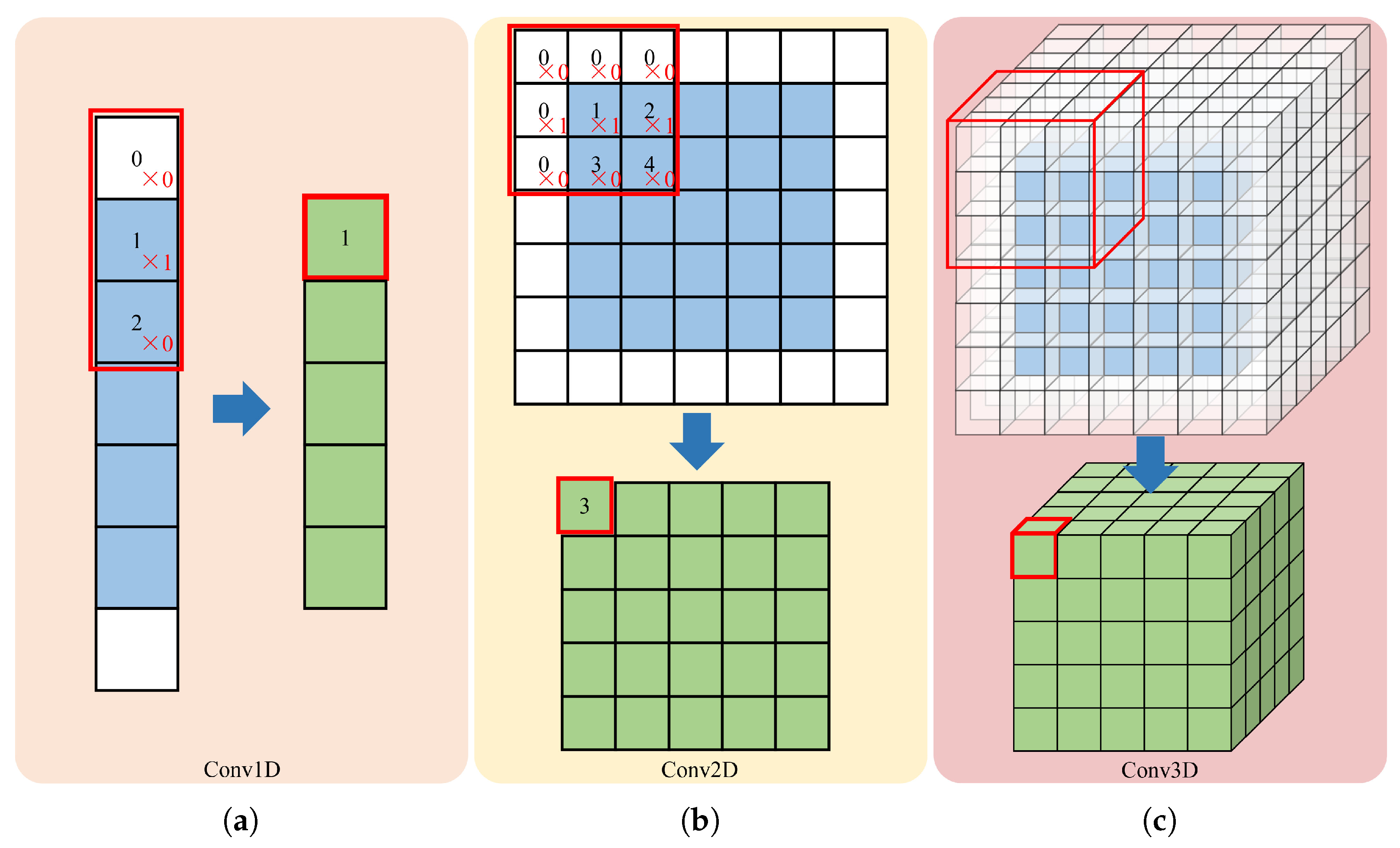
By formulating LFR as a DL-based regression problem, we evaluate a 3D CNN-based approach for LFR with the following motivations. Previous works are based on either 1D or 2D CNNs. Consequently, seismic data are processed slice-by-slice [8], trace-by-trace [4], or shot-by-shot [26]. However, shot gathers of a prestack line are 3D field seismic data. In this work, the 3D seismic data actually refers to the prestack line data (2D) with the source as the third axis, i.e., ($n_{time}$, $n_{rec}$, $n_{src}$), instead of the conventional 3D seismic data ($n_{time}$, $n_{rec}^x$, $n_{rec}^y$), where $n_{time}$, $n_{rec}$, and $n_{src}$ denote the number of the time sampling points, the receivers, and the sources, respectively. $n_{rec}^x$ and $n_{rec}^y$ represent the number of receivers along the space in the x- and y-directions, respectively. One drawback of previous DL-based 1D/2D reconstruction methods is that the stack of the prediction errors diminishes the correlation of events among slices/traces/shots. Previous 1D/2D reconstruction methods cannot fully exploit information that is available in 3D seismic data (see Figure 1). Three-dimensional reconstruction based on 3D CNN can overcome this problem by utilizing spatial information naturally available in 3D seismic data. Three-dimensional CNN can inherently use this additional information to produce better results with superior spatial consistency and accuracy. This work is thus closely related to the work of Ovcharenko et al. [8], Sun and Demanet [4], and Fang et al. [26]. In addition, suppressing the Gibbs effect associated with the hard splitting of the low- and high-frequency data is lightly discussed in the previous work. This work is essentially based on the works of Chai et al. [14], Chai et al. [18], and Chai et al. [19], where 3D CNN was applied to 3D data reconstruction, multitrace deconvolution, and geophysics-steered self-supervised learning for deconvolution, respectively. The work combines and extends the ideas proposed earlier. Open-source work in the LFR area is scarce. For reproducibility, we have made all materials related to this work open-source.

We organize the rest of the paper as follows. First, we describe how we split the low- and high-frequency data regarding the Gibbs effect. Then, we briefly describe the underlying DL methodology. Next, we detail the 3D CNN architecture used for LFR in this research, which is based on U-Net [29] and Bridge-Net [19,24]. Then, we provide the CNN training setup in detail. A three-dimensional CNN is trained to reconstruct missing low frequencies from raw high frequencies in the time domain. Then, we report the CNN training stage’s convergence and the impact of different convolutional kernel sizes. After testing CNN’s effectiveness on the Marmousi2 open dataset [30], we use a field dataset, which is invisible during the training stage, to check CNN’s generalization capability. We compare the result of 2D and 3D CNNs to show the benefits of our approach. We then assess the LFR results in terms of FWI with the aid of an open-source FWI code package PySIT [31], to check whether the predicted low frequencies are accurate enough to mitigate FWI’s cycle-skipping problems and to observe the impact of low frequencies on the FWI results.

2. Methods

2.1. Splitting the Low- and High-Frequency Data

For better understanding, we elaborate on how we split the low- and high-frequency data in detail with the aid of Figure 2 and Figure 3. For illustrative purposes, we split the data above 5 Hz and below 5 Hz. Taking the trace seismogram shown in Figure 2a as an example, we first transform the seismogram into the Fourier domain (see Figure 2b). Then, we set the high frequencies ≥5 Hz (and their conjugate symmetry components) of the Fourier spectra to be zero (see Figure 2d). We inverse transform the HF zero-filled spectra into the time domain to obtain the LF data (see Figure 2c). Similarly, we set the low frequencies <5 Hz (and their conjugate symmetry components) of the Fourier spectra to be zero (see Figure 2f). We inverse transform the LF zero-filled Fourier spectra into the time domain to obtain the HF data (see Figure 2e). We coined this splitting process as the “hard” splitting of the low- and high-frequency data.

We can clearly see the Gibbs effect associated with the hard splitting of the low- and high-frequency data in Figure 2c,e, which is lightly discussed in the previous work, e.g., [4,26]. When only part of the frequencies is used in the reconstruction, each edge shows ringing (decaying oscillations). This ringing phenomenon is known as the Gibbs effect. The ringing phenomenon in Figure 2c,e is undesirable for LFR. As a consequence, we designed a Hanning-based window for suppressing the Gibbs effect associated with the hard splitting of the low- and high-frequency data. The Hanning window [32] is a taper formed by using a weighted cosine. The Hanning window is defined as:

$$w\left(n\right)=0.5-0.5cos\left(\frac{2\pi n}{M-1}\right)0\le n\le M-1,$$

(1)

where M is an integer, denoting the number of points in the output window. Equation (1) returns the coefficients of the Hanning window, with the maximum value normalized to one, and the value one appears only if M is odd.

Figure 2g,h shows the designed Hanning-based window for suppressing the Gibbs effect. Figure 2j,l displays the Fourier amplitude spectra of the low- and high-frequency data after applying the designed Hanning-based window. Figure 2i,k shows the low- and high-frequency signals after applying the designed Hanning-based window. We can see that the Gibbs effect shown in Figure 2c,e is successfully suppressed in Figure 2i,k by the designed Hanning-based splitting window shown in Figure 2g,h. Figure 3 is provided for a shot gather 2D view of the Mobil AVO Viking Graben Line 12 dataset [33,34]. For the field dataset shown in Figure 3a, Mobil oil company released this 25 km line to the public in 1994. The seismic line dataset includes 1001 shot gathers; each shot gathers for 6 s on 120 receivers at a time, with a sampling interval of 4 ms. The shot and receiver intervals are 25 m, and the common-midpoint spacing is 12.5 m. The nearest offset is 262 m, and the farthest offset is 3237 m [33]. For more information about the dataset, please refer to Madiba and McMechan [33] and Keys and Foster [34]. Please note that the Gibbs effect shown in Figure 3b,c is also successfully eliminated in Figure 3d,e by the designed Hanning-based splitting window. We called this Hanning-based splitting process as the “soft” splitting of the low- and high-frequency data.

When doing “hard” splitting, we explicitly set zeros to the target parts of the spectrum, thus ensuring that no spectral leakage from input to targets occurs. When applying the “soft” filtering, we should also ensure that no signal leaks to the targets for training. Please note that there is no signal leakage from input (i.e., Figure 2a) to targets (i.e., Figure 2i,k) because after we generate the Hanning-based splitting window for HF (i.e., Figure 2h), we use one minus the Hanning-based splitting window for HF to yield the Hanning-based splitting window for LF (i.e., Figure 2h). Therefore, the sum of the target signals in Figure 2i,k can completely reconstruct the input signal in Figure 2a with no signal leakage. The designed Hanning-based window in Figure 2h can ensure that the input data to the network is cleared from target low-frequencies (e.g., 5 Hz). These are the merits of the designed Hanning-based window.

Figure 3. Splitting the low- and high-frequency data (shot gather 2D view). (a) A shot gather of the Mobil AVO Viking Graben Line 12 dataset [33,34]. (b) Hard split LF (<5 Hz) data in the time domain. (c) Hard split HF (≥5 Hz) data in the time domain. (d) Soft split LF data in the time domain. (e) Soft split HF data in the time domain. Panels (f–j) show the Fourier amplitude spectrum of the data shown in panels (a–e), respectively. Note that the Gibbs effect shown in panels (b,c) is successfully eliminated in panels (d,e) by the designed splitting window. There are artifacts formed at the bottoms of subfigures (b,d), which are caused by the sudden cutoff in the time domain. Those artifacts can be further suppressed by applying a smooth tapering calculated by Equation (1).

Figure 3. Splitting the low- and high-frequency data (shot gather 2D view). (a) A shot gather of the Mobil AVO Viking Graben Line 12 dataset [33,34]. (b) Hard split LF (<5 Hz) data in the time domain. (c) Hard split HF (≥5 Hz) data in the time domain. (d) Soft split LF data in the time domain. (e) Soft split HF data in the time domain. Panels (f–j) show the Fourier amplitude spectrum of the data shown in panels (a–e), respectively. Note that the Gibbs effect shown in panels (b,c) is successfully eliminated in panels (d,e) by the designed splitting window. There are artifacts formed at the bottoms of subfigures (b,d), which are caused by the sudden cutoff in the time domain. Those artifacts can be further suppressed by applying a smooth tapering calculated by Equation (1).

2.2. Basic Theory of DL

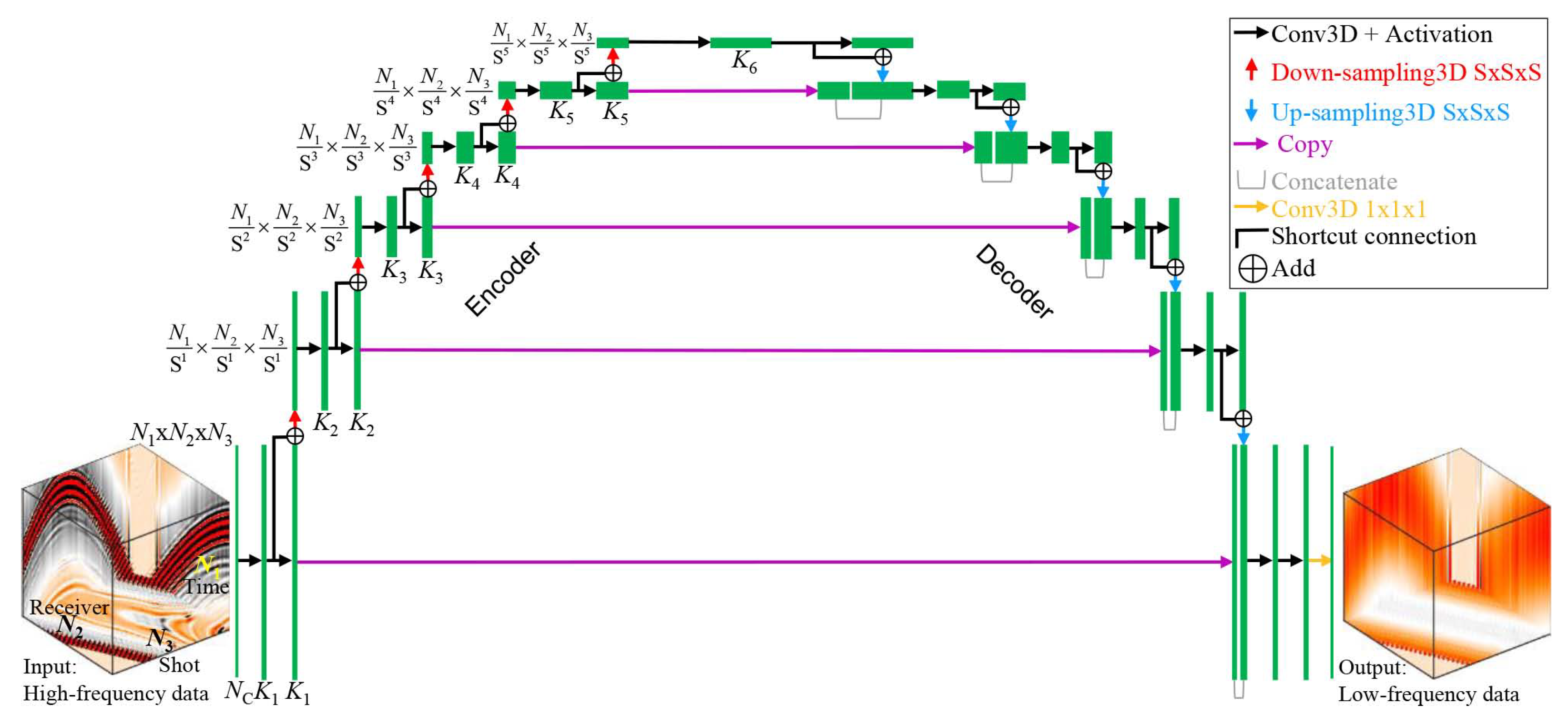
We regard CNN as a bridge linking the input $\mathbf{X}$ (e.g., HF data, see Figure 4, lower left) and the target ${\mathbf{Y}}_{\mathrm{ref}}$ (e.g., LF data, see Figure 4, lower right). For LFR, the input-output pairs are time-domain seismograms. CNN is a type of ANN in which some of the hidden layers are convolutional. CNN takes advantage of numerous transforming layers to extract features. Each convolution operator is applied to a subdomain of $\mathbf{X}$. Therefore, it is the summation of a part of the input weighted by the convolutional kernel. After numerous transformations, CNN integrates learned feature maps in the last layer to predict ${\mathbf{Y}}_{\mathrm{pre}}$. For the sake of brevity, DL is approximated as function f

$${\mathbf{Y}}_{\mathrm{pre}}=f_{\theta }\left(\mathbf{X}\right),$$

(2)

where $\theta$ denotes CNN parameters (i.e., weights, biases). The universal approximation theorem implies that CNN can express an arbitrary function up to the target precision when it possesses enough hidden layers and parameters [4].

CNN’s parameters are optimized for regressing low frequencies from high frequencies. CNN evolves by updating $\theta$ to minimize a loss function $\varphi \left(\theta \right)$ that measures how close ${\mathbf{Y}}_{\mathrm{pre}}$ is to ${\mathbf{Y}}_{\mathrm{ref}}$. The parameters are updated by backpropagation of the errors utilizing automatic differentiation [35] and optimization algorithms, e.g., the Adam optimization algorithm [36]. For a complete elaboration of CNN, ANN, or DL, please refer to an excellent textbook written by Goodfellow et al. [37].

2.3. The CNN Architecture

Figure 4 shows the 3D CNN architecture for LFR of shot gathers of a prestack line. Similarly, we replace the 3D convolutional/pooling/upsampling layers of 3D CNN with their 2D counterparts to build 2D CNN trained for LFR of a shot gather (i.e., a 2D matrix). The architecture of the to-be-trained ANNs is mature since it has been widely used in our previous works, e.g., [13,14,18,24]. The CNN architecture in Figure 4 is employed for irregular and regular missing 3D seismic data interpolation [14], multitrace deconvolution [18], and geophysics-steered self-supervised learning for deconvolution [19]. A two-dimensional CNN was adopted by Chai et al. [13] for 2D seismic data reconstruction and Chai et al. [24] for seismic facies classification. The architecture in Figure 4 is mostly the same as the one evaluated in Chai et al. [24], except for the final output layer. For completeness of this paper, we briefly transcribe some key information about the architecture from Chai et al. [24]. For more details, please refer to Chai et al. [24]. In Figure 4, the green boxes denote extracted features. The green boxes possessing the same width have the same number of features. The green boxes possessing the same height have the same height, width, and depth sizes of features. CNN includes an encoder and a decoder, where the encoder uses the available high frequencies as input and gradually calculates multilevel features, and the decoder successively composes the LFR counterparts starting from the large-scale features and continuing to fine-scale features. The arrows with different colors delegate different operators. The encoder comprises repetitive applications of padded convolutional layers, where each convolutional layer is followed by an activation layer (black arrow). The decoder contains an upsampling layer (blue arrow), followed by a concatenation layer with the copied encoding features (purple arrow), and repetitive convolutional layers, where each convolutional layer is followed by an activation layer. Finally, we use a $1\times 1\times 1$ convolutional layer (green arrow) for projecting features to the LFR target.

Inspired by the ResNet proposed by [38], Chai et al. [24] enhanced the standard U-Net [29] by adding shortcuts immediately before each pooling/upsampling operation, which can theoretically ease the notorious problem of vanishing/exploding gradients. For practical implementation, we write our code in Python and use Keras with a TensorFlow backend. Based on our previous experience with the evaluated CNN architecture [13,14,18,19,24], we use max-pooling for the pooling layer and a rectified linear unit (ReLU) for the activation layer, yielding elementwise $max(\mathbf{x},0)$, where $\mathbf{x}$ represents a tensor. Moreover, we can also utilize strode convolution instead of max pooling, which is proven to deliver better results since no information is lost during downsampling.

3. Experiments on Low-Frequency Reconstruction

3.1. Training Setup

3.1.1. Computing Environment

Owing to the specifications of the CNN model (e.g., convolutional kernel number $K_{i,i\in [1,6]}$ in Figure 4) and training settings that are limited by hardware, e.g., graphics processing unit (GPU), our computational resources are summarized as follows: an Intel(R) Xeon(R) W-2223 3.60 GHz CPU, an NVIDIA TITAN RTX 24 GB GPU, and RAM 128 GB. The number of convolutional kernels ($K_i$) increases (e.g., $K_1$ = 16, $K_2$ = 32, $K_3$ = 64, $K_4$ = 128, $K_5$ = 256) after each downsampling operation.

3.1.2. Synthetic Data Generation and Pre-Processing

Preparing training data implies gathering/simulating seismic datasets with various geological models. For field data, we have no actual LFR labels. Hence, we prepare training pairs only using synthetic datasets. For good generalization, the models employed to generate training data pairs should be capable of representing numerous underground conditions containing various structures. This will ensure that the CNN is capable of finding representative parameters for addressing datasets from various scenarios/regions. The publicly available Marmousi2 synthetic dataset [30] is a good candidate. We directly use the open-source Marmousi2 shot gathers. To address geometry, the grid size of the velocity model is 2801 × 13,601 and the grid space $dx$ = $dz$ = 1.25 m. The source is a synthetic air gun, and the firing depth is 10 m. The source interval is 25 m [30]. The source is a 5-10-60-80 Ormsby zero-phase wavelet. “Streamer” cables measure the hydrophone pressure at 1361 positions, and the group interval is 12.5 m. The cable is fixed at a depth of 5 m and is also fixed in space during acquisition. Martin et al. [30] simulated 480 shots, 1361 receivers per shot, and 2500 points per trace. The time interval $dt$ is 2 ms, and the record duration of the raw data is 5 s, which is adequate to record reflections and other waves that arrive earlier than direct arrivals at far offsets. For more details about this dataset, please see Martin et al. [30].

Because seismic data amplitudes range broadly, they should be balanced. The reflection energy is weaker compared to that of direct arrivals. When we immediately feed normalized data into CNN, contributions of reflections to CNN’s training are relatively weak, reducing CNN’s accuracy. Consequently, the first arrivals are muted before splitting into high and low frequencies. For first-arrival removal, we build the muting mask by picking water bottom bounces, which is relatively easy for the Marmousi2 model since its water bottom is flattened. As a result, we muted the first arrivals before performing the LFR test. Currently, other strategies to balance the amplitude are not employed.

To generate enough data pairs, we divide the entire dataset into substantial small datasets of a fixed shape (e.g., $64\times 64\times 64$, $n_{time}\times n_{rec}\times n_{src}$, the equivalent dimensions in seconds and meters are 0.256 s × 800 m × 1600 m). The time sampling is not too sparse (4 ms). However, the recording duration is slightly short (256 ms). The cube size is inspired by the size used in the work of Fang et al. [26], where the size of the input data patches is $64\times 64$. There is an overlap of 10 between two of the small datasets. Next, we split seismograms above 5 Hz and below 5 Hz for synthesizing CNN’s input-output pairs. Because forward and inverse Fourier transforms are intensively computed while splitting low and high frequencies, we recommend the CuPy package for fast Fourier transform (FFT), which can significantly accelerate the splitting process. CuPy is a library compatible with NumPy multi-dimensional array implemented on compute unified device architecture (CUDA). CuPy contains the complete FFT functions available in NumPy and a subset in SciPy. It is a great use case of GPU computation, and the readers can see this from the shared code.

The training sample size is $64\times 64\times 64$ along the time ($n_{time}$), receiver ($n_{rec}$), and shot ($n_{src}$) axes, respectively (see Figure 5) and the batch size is 40. Finally, we prepare a total of 8000 data pairs that are used as a training dataset and 465 data pairs that are used as a validation dataset. To sum up, we used the public data ($n_{time}$, $n_{rec}$, $n_{src}$) for the Marmousi2 model and split it into 8000 cubes of ($64\times 64\times 64$). Figure 5 displays six input-output training pairs. Normalizing input-output pairs within the dataset is important for the successful training of many DL models. Appropriate normalization of training pairs expedites training and balances the contributions of each data pair. We scale each of the input-output training data pairs individually with the maximum absolute value of the corresponding shot gathers. We save the scaling coefficients for restoring amplitudes to the raw scale to facilitate subsequent processes.

3.1.3. Evaluation Metrics

During the training stage, a mean squared error (MSE) loss function is used. We train CNN utilizing the Adam algorithm. The learning rate is 0.0001. We utilize the early stopping strategy to prevent overfitting. We use S/N, which is defined as

$$\mathrm{S}/\mathrm{N}\left(\mathrm{dB}\right)=-20{log}_{10}\frac{{∥{\mathbf{Y}}_{\mathrm{ref}}-{\mathbf{Y}}_{\mathrm{pre}}∥}_2}{{∥{\mathbf{Y}}_{\mathrm{ref}}∥}_2},$$

(3)

to evaluate the quality of the LFR result, where ${∥\mathbf{X}∥}_2$ returns the 2-norm of $\mathbf{X}$. In addition, we also use MSE, which is explicitly defined as

$$\mathrm{MSE}=\mathrm{mean}\left({∥{\mathbf{Y}}_{\mathrm{ref}}-{\mathbf{Y}}_{\mathrm{pre}}∥}_2\right),$$

(4)

to evaluate the error of the LFR result, where $\mathrm{mean}\left(\mathbf{X}\right)$ returns the mean value of the elements in $\mathbf{X}$.

3.2. Convergence of the CNN Training Stage

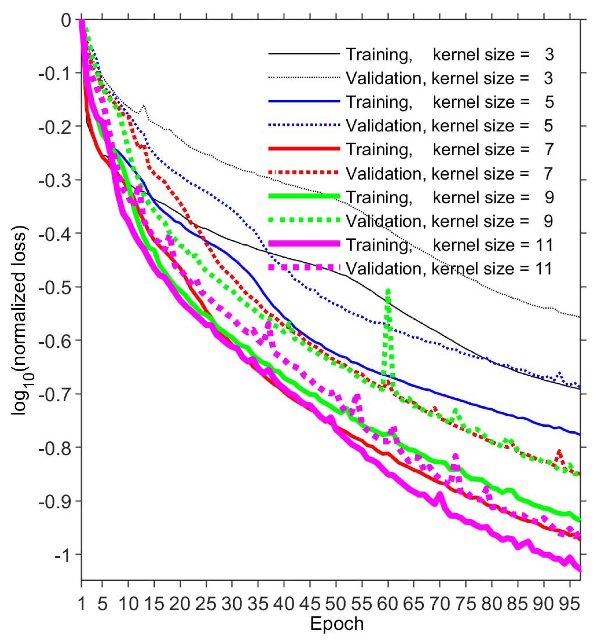
Convergence is the first and foremost issue for CNN’s training stage. Therefore, Figure 6 is provided, indicating that the training stage’s convergence rate is influenced by convolutional kernel size. Training and validation losses for different kernel sizes decay with the training epochs, which indicates CNN training’s convergence and that CNN is not overfitting the data. It is anticipated that the loss values of the training dataset are smaller compared to those of the validation dataset (In Figure 6, this is represented by solid curves versus dotted curves) because the training stage is driven by the training data fitting. The validation data do not contribute to the CNN’s update. It looks like training is not complete in Figure 6. However, the validation accuracy is acceptable. Therefore, we use the early stopping strategy to prevent overfitting.

For all of the shown cases, we observe a meaningful phenomenon. That is, the larger the kernel size is, the faster the convergence rate (see Figure 6). That is, a large kernel size helps convergence during training. We provide the following explanations. A neuron’s receptive field is an essential hyperparameter for LFR with DL, which corresponds to the input data’s local region impacting this neuron’s response. This connectivity’s spatial extent is associated with the size of the convolutional kernel. We can employ a larger convolutional kernel to enlarge the CNN’s receptive field. Reasonably larger kernels enable CNN sufficient freedom for the reconstruction of long-wavelength low frequencies. Thus, we have valid reasons to expect that CNNs with a reasonably larger kernel size should generate better LFR results. This point is partly supported by the following Figure 7 and Figure 8. However, we need to underline that employing a large kernel size helps convergence during training at the cost of a higher computational cost.

3.3. Training and Validation on Synthetic Open Datasets

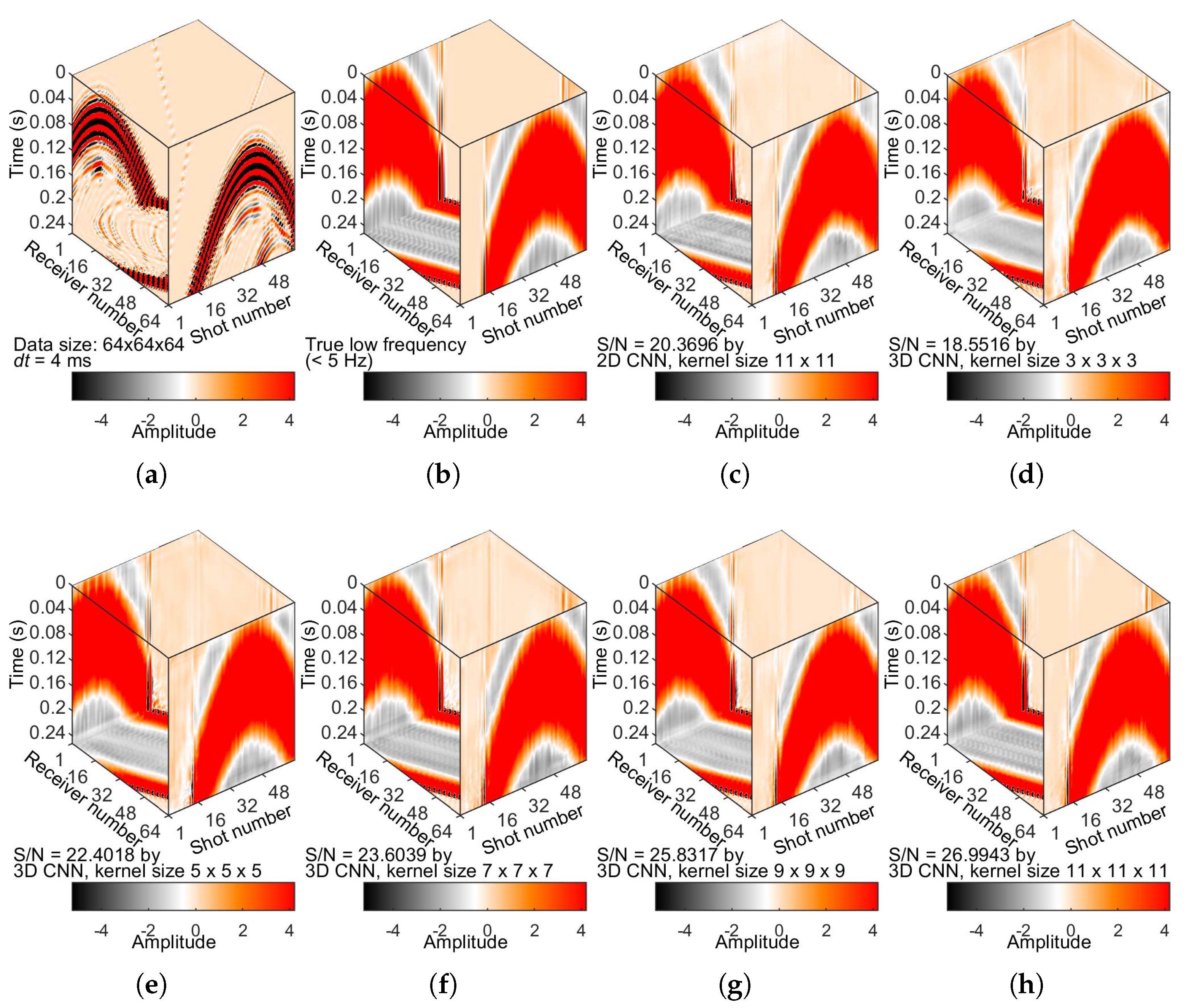
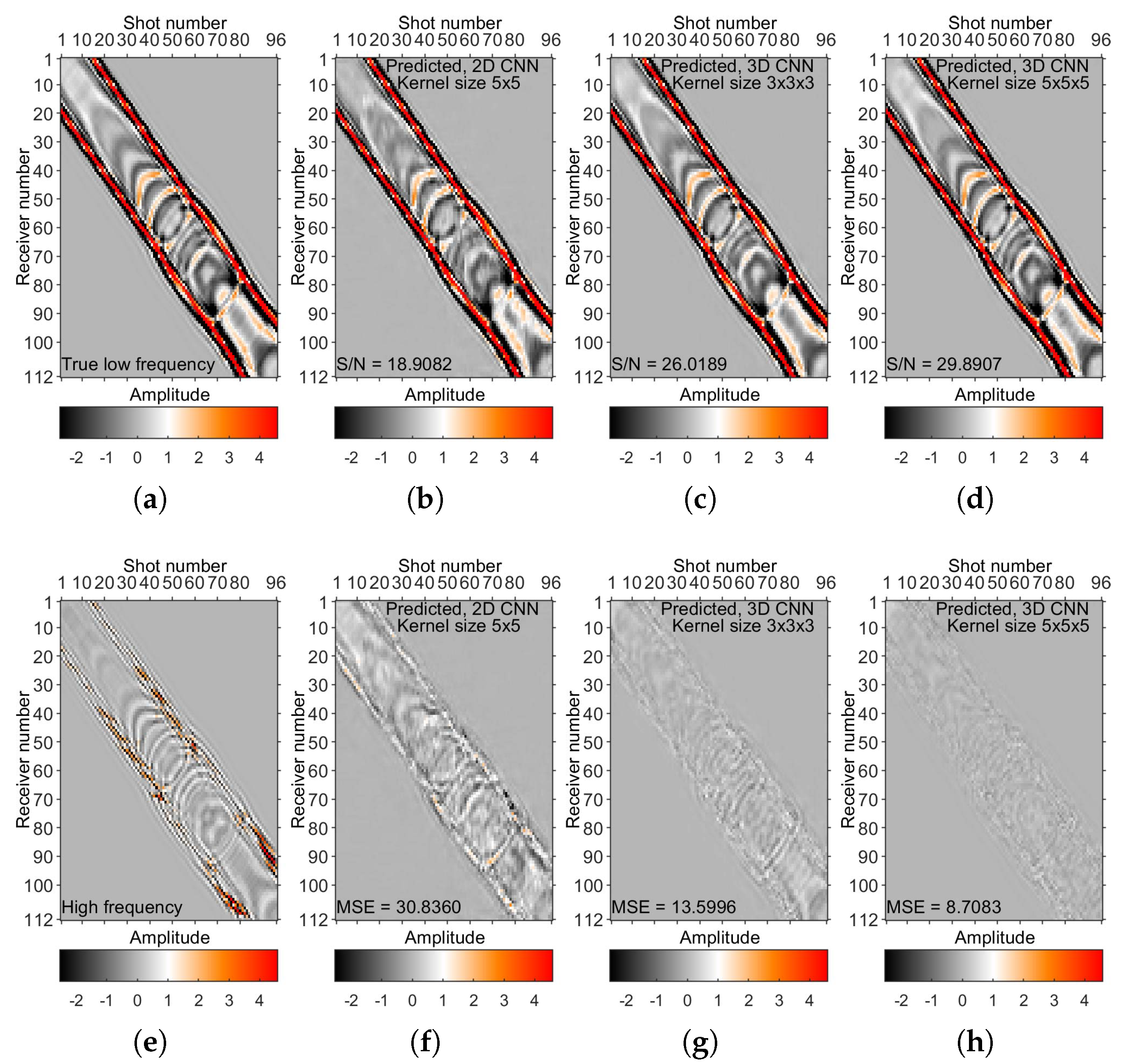
We validate CNN’s ability to reconstruct low frequencies on the Marmousi2 open dataset (Figure 7). In the training stage, the CNN’s input is confined to a fixed size of $64\times 64\times 64$. However, this restriction no longer exists for tests. Shot gathers of a prestack line can be fed into the 3D CNN directly. The dataset in Figure 7 is unseen in the training stage. In Figure 7b,h, the LFR data are in accordance with the actual low frequencies. The reconstructed results in Figure 7h show that the trained CNN model is capable of precisely predicting seismograms in the LF band. CNN is able to mine intricate relations between low and high frequencies.

Figure 7 also demonstrates that 3D CNN works better than 2D CNN in terms of accuracy for LFR of shot gathers of a prestack line. For 2D experiments, we did not apply 2D CNN to 3D volumes. Instead, we use 2D samples in 2D CNN experiments. To generate the 2D CNN prediction in Figure 7c (and in Figure 9c), we feed each shot gather into the trained 2D CNN model one by one using the same settings as the 3D model. That is, shot gathers of a prestack line are processed by 2D CNN in a shot-by-shot manner. A comparison of Figure 7c,h reveals the disadvantages of the DL-based 2D CNN LFR method and, thus, the benefits of the DL-based 3D CNN LFR method by considering additional information. Three-dimensional CNN is capable of adequately exploiting seismic data’s 3D nature, and extra-dimensional information is beneficial to LFR.

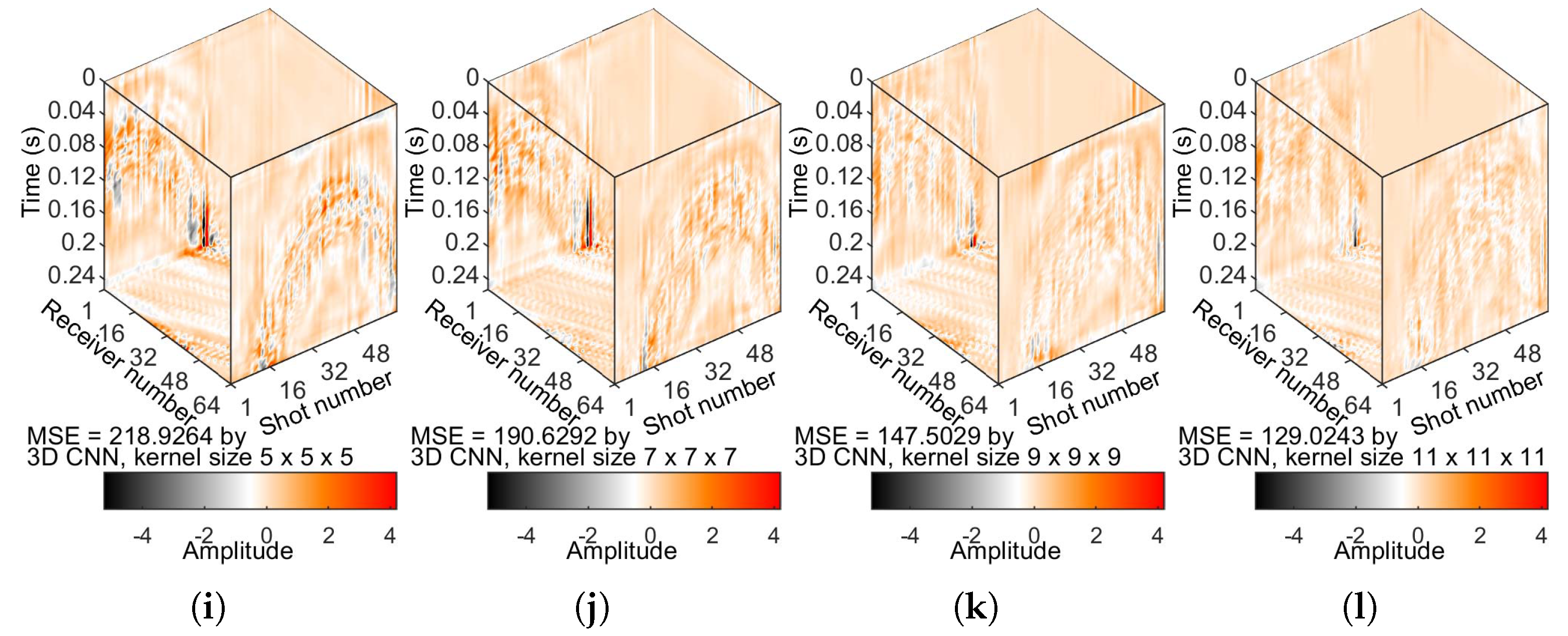
Comparing the SNRs (and the MSE values) in Figure 7 and Figure 8, our hypothesis that CNN with a reasonably larger kernel size generates a better LFR result in terms of accuracy is supported. In general, larger convolutional kernels imply a stronger learning ability because larger kernels extend the receptive field. Generalization performance is thus improved to some extent. However, we need to emphasize that the bouncing phenomena of the curves for kernel sizes of $9\times 9\times 9$ and $11\times 11\times 11$ imply that larger kernel sizes (i.e., larger trainable parameters) increase the difficulty of training CNN. The stability of the training process is affected by the convolutional kernel size.

3.4. Test on a Field Dataset

For verifying whether CNN is capable of really generalizing “out of sample”, where training and test scenarios are significantly disparate, we train the model using data pairs gathered from the Marmousi2 open dataset. However, we now test the model on a field dataset, i.e., the Mobil AVO Viking Graben Line 12 dataset [33,34] (see Figure 9). This dataset is completely unseen in the CNN’s training stage. This dataset contains 256 shots, 32 receivers for every shot, and 96 points for every trace. Both the shot and receiver intervals are 25 m, $dt=$ 4 ms [34]. Usually, we have to apply similar pre-processing of the training process to enable “domain adaptation/transfer learning” for an unseen dataset. For field data applications, we did not pre-process the downloaded field data, except for muting the first arrivals on field data and normalizing the data by the max value of the absolute value of the data to fit the range [−1, 1]. How to accurately deal with new source wavelet remains an open issue. For the spectral plots shown in Figure 10, the power spectra in dB are calculated by

$$\mathrm{Spec}\left(\mathrm{dB}\right)=20{log}_{10}\frac{\mathbf{x}}{\mathrm{mean}\left(\mathbf{x}\right)},$$

(5)

where $\mathbf{x}$ denotes the Fourier spectral amplitude of a signal.

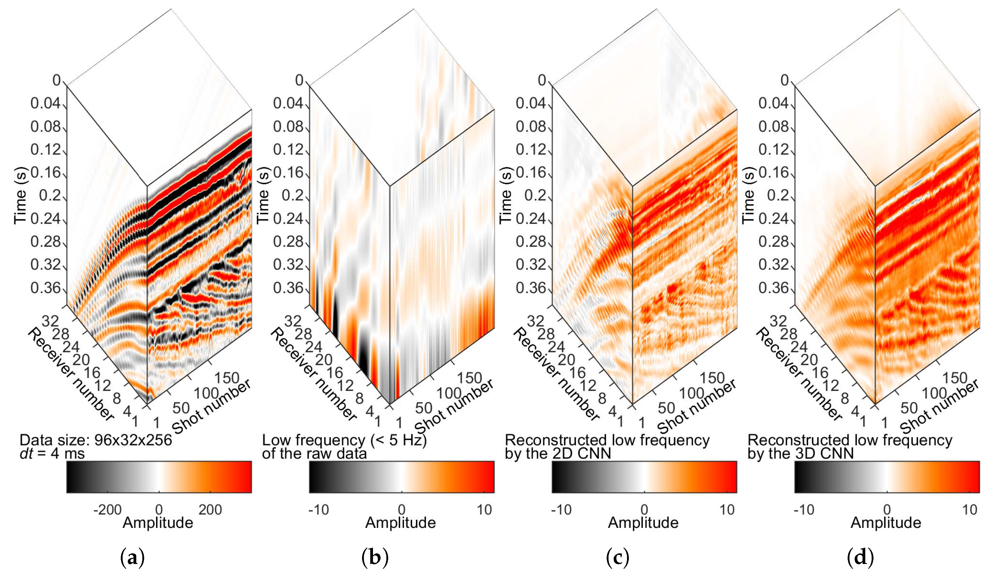
There are almost no LF events in the raw data (see Figure 9b). From the spectra of the bandlimited data (Figure 10a), records in low frequencies are almost completely missing. Low frequencies (e.g., <5 Hz) are relatively weak, as shown in Figure 10a. We observe from Figure 9d that the trained 3D CNN predicts highly relevant low frequencies from raw data. The low frequencies are extended, as shown in Figure 10b. We think the spectrum shown in Figure 10b is reasonable. The results imply that the trained 3D CNN model can recover low frequencies from high frequencies. Comparisons of Figure 9c,d suggest the disadvantage of the 2D CNN LFR method and the advantage of the 3D CNN LFR method. Although we do not have the true answer for field data, we believe the LFR result of 3D CNN outperforms that of 2D CNN in terms of the highly relevant LF events. The additional dimension contributes to the LFR result. The evaluated architecture has sufficient generalizability to reconstruct low frequencies of waves that are fully absent in the training phase.

For field data, we do not have an initial model for FWI and do not have a reference FWI solution to understand how good the predicted low frequencies are. Therefore, we cannot show the FWI results. We rely on synthetic data to evaluate the LFR quality in terms of FWI.

4. Low-Frequency Reconstruction for Full-Waveform Inversion

Now, we evaluate the quality of the reconstructed low frequencies in terms of FWI, which is the key motivation of LFR. We evaluate the LFR quality by running FWI on a benchmark Marmousi model [39]. The default Marmousi model is not modified. We take advantage of the open-source FWI code package PySIT [31] to accomplish this task. For technical aspects, the wave equation used is the time-domain constant-density acoustic wave equation. In the wave equation forward modeling process, the spatial accuracy order is six. The used codes evaluate the least squares objective function over a list of shots. Therefore, the used code package belongs to the ${\ell }_2$ norm-based FWI. In this work, we used the FWI method developed by Hewett et al. [31], and we did not work on proposing a new FWI method. We mainly focus on achieving low-frequency reconstruction via deep learning. As a consequence, comparing our FWI results with traditional approaches, such as another ${\ell }_2$ norm-based FWI [40], is not in the scope of this paper. We used the limited-memory BFGS (LBFGS) method [41] for the large-scale optimization process. That is, for the calculations of adjoint sources, the codes compute the L-BFGS update for a set of shots.

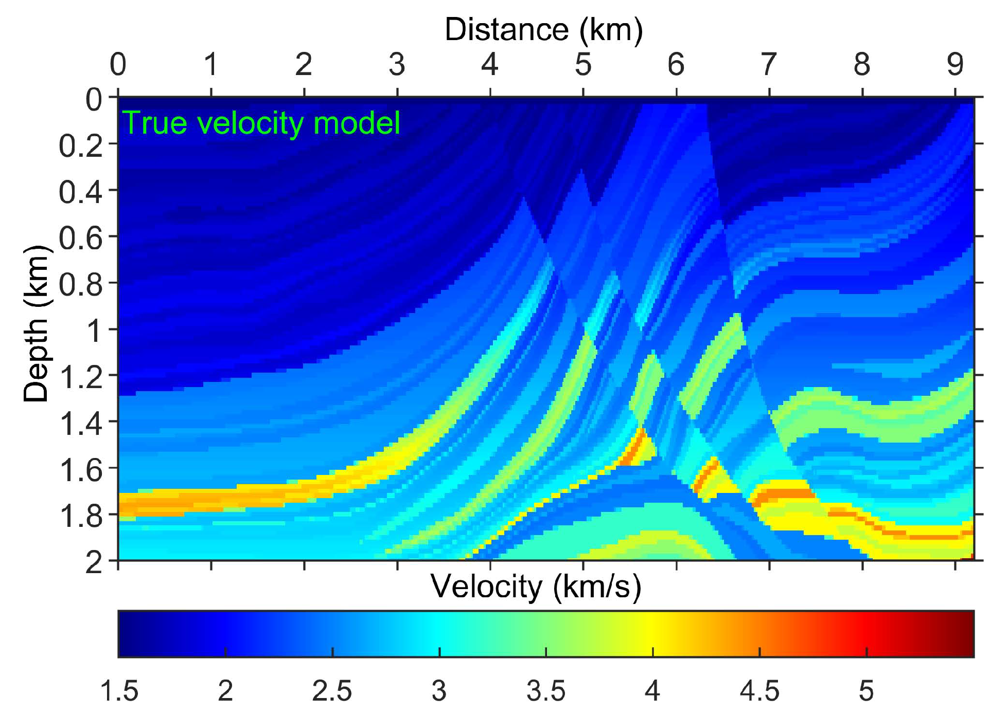
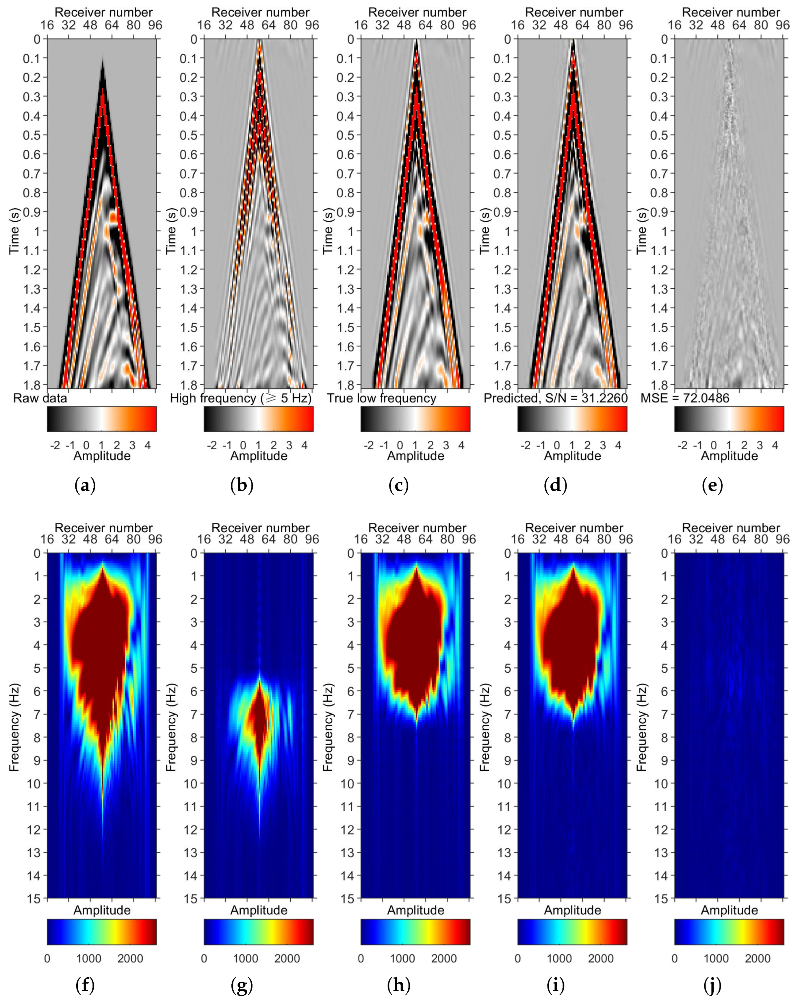
We simulate the shot gathers (Figure 11a) on the Marmousi model (Figure 12). For data modeling and FWI, we use the default settings implemented in PySIT [31]. The grid size of the velocity model is $151\times 461$, and the grid space is $dx$ = $dz$ = 20 m. We use a 10-Hz Ricker wavelet. The source depth is 15 m, and the receiver depth is 0 m. We finally simulate 96 shots, 112 receivers per shot, with an equispaced geometry. There are 3008 points per trace, $dt\approx$ 0.0006 ms. We divide the complete data volume with a size of $3008\times 112\times 96$ into smaller datasets with a size of $1504\times 96\times 96$. There is an overlap of eight between two small samples.

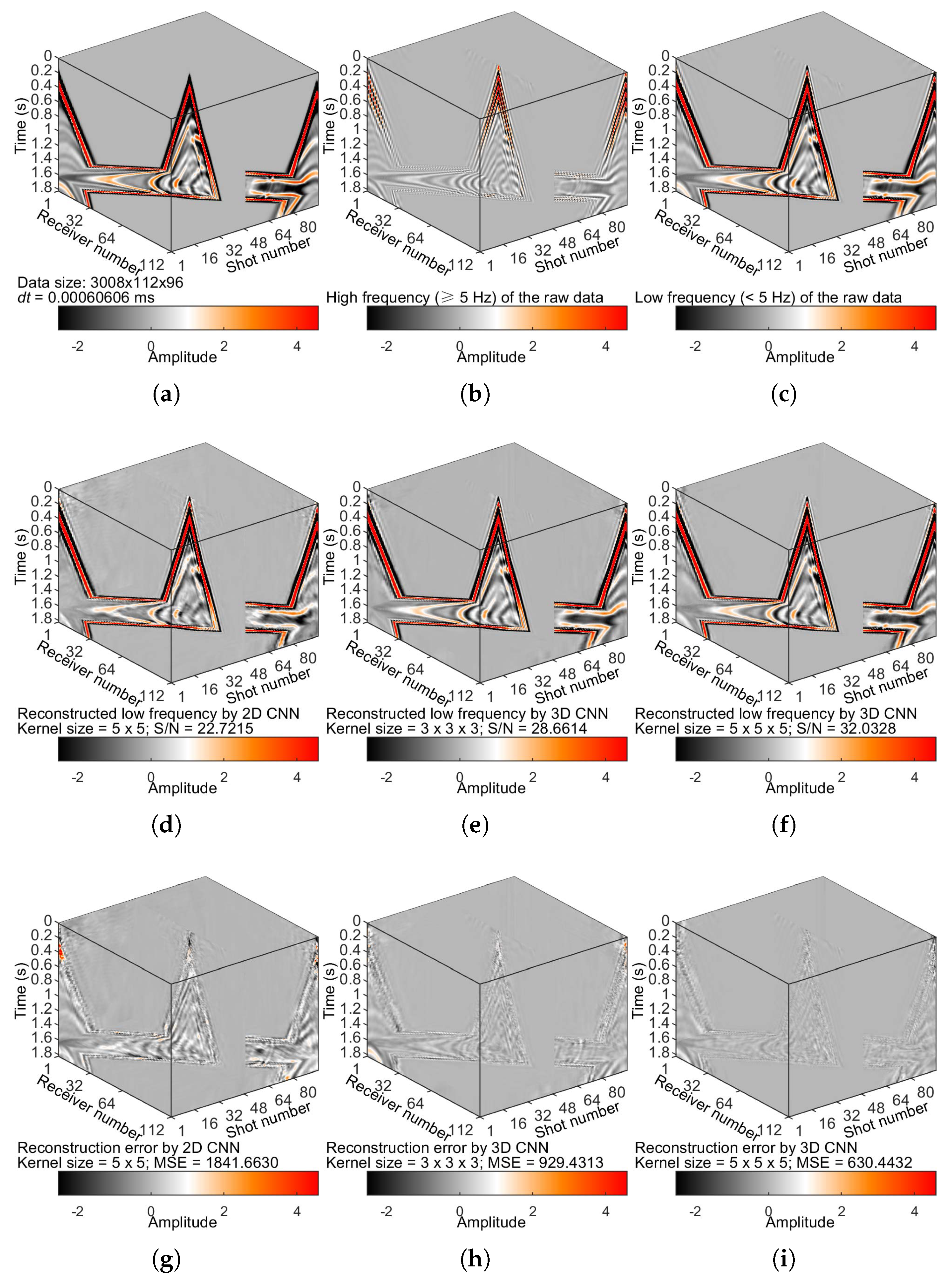
Figure 13 shows the S/N and MSE values. Figure 11e,f shows the DL-predicted low frequencies by 3D CNN with different kernel sizes. Figure 14 shows a time slice view at 1.2121 s of the 3D data volumes shown in Figure 11. Figure 15 displays a shot gather view of the 3D data volumes shown in Figure 11. The DL-predicted low frequencies with a kernel size of $5\times 5\times 5$ (Figure 11f) are superior to the results of $3\times 3\times 3$ (Figure 11e), reflected in the S/N and MSE values (see also Figure 13). Figure 11d,f shows the DL-predicted low frequencies by 2D CNN and 3D CNN, respectively. The DL-predicted low frequencies by 3D CNN (Figure 11f) are superior to the results of 2D CNN (Figure 11d), embodied in the S/N and MSE values. We reconfirmed the importance of a larger kernel size to capture low frequencies.

As a bandwidth extension method, we also compare the reconstructed and actual low frequencies in the frequency domain for shot comparison (Figure 15). We show the result with far offsets and later arrival times in Figure 15. The results in Figure 11 and Figure 15 show that the developed method has adequate accuracy. Figure 16 shows the frequency-wavenumber (F-K) amplitude spectra of the data shown in Figure 15a, which indicates these plots in Figure 15 are not aliased.

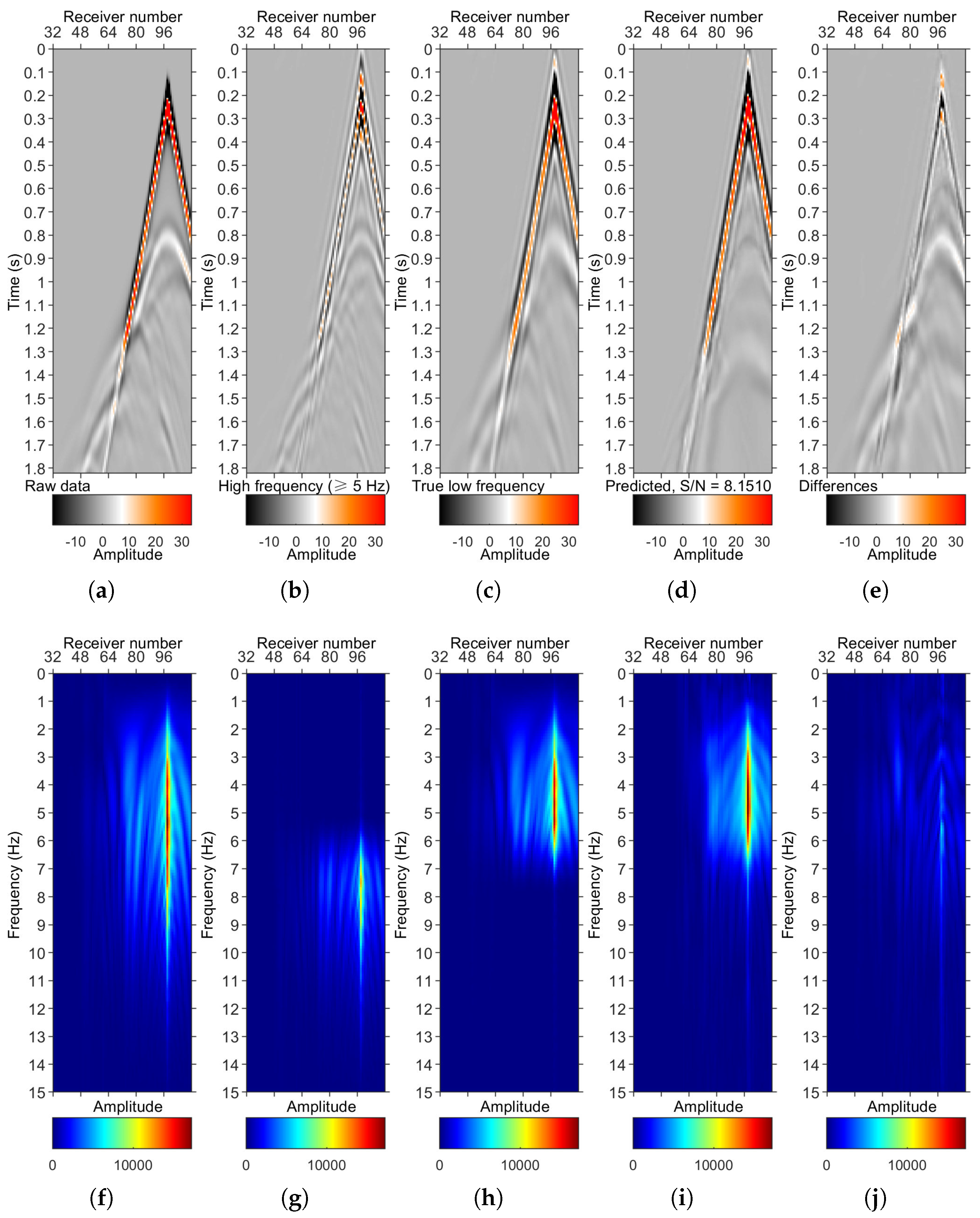
Figure 17 shows the test of the method on another completely unseen BP 2004 benchmark model [42] other than the Marmousi1 model, which is already used in the training process. It is more helpful to sustain the generalization ability of the proposed method. We observe that the accuracy of the LFR result of the unseen BP 2004 benchmark model is lower than that of the Marmousi1 model used in the training process. This is as expected. The main reasons are as follows. It is likely due to the lack of diversity in the training dataset, which is built of crops from the Marmousi model. The training is biased toward the Marmousi1 model since the NN was trained on data generated on patches of this model. Even when crops are randomly sampled from the data/model, they still encode proper geological contrasts present in the Marmousi1 benchmark model. This partly supports the generalization ability of DL. It raises concerns about the sufficiency of the training dataset to enable the inference of previously unseen data. It also indicates the significance of augmenting the training dataset’s diversity for supervised-learning-based methods because exposing CNN to a wider scope of situations is the most effective way to enhance the generalization ability of DL. Moreover, the generalization capability (or aiming to reach superior generalizability in LFR) is undoubtedly important. However, it is not the core task of this work. The generalization ability of nearly all of the supervised-learning-based methods is limited. The data generation mechanism can be enhanced. Training the CNN on a larger dataset generated from tremendous various models is a sound approach, which is left as future work.

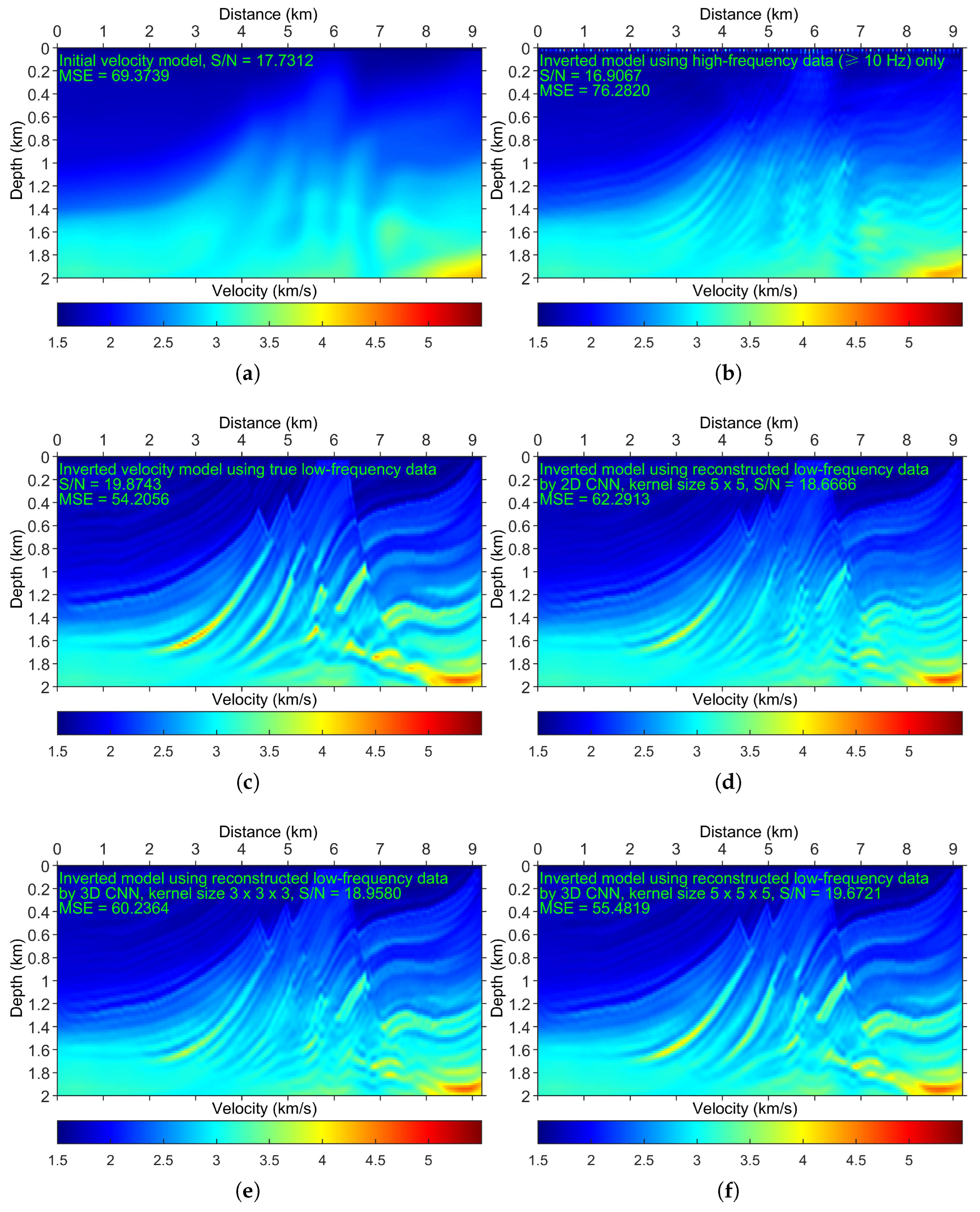
Figure 18 displays the results of low frequencies applied to FWI. The initial model shown in Figure 18a is not accurate enough. A comparison of Figure 18b (the FWI result using only high frequencies) and Figure 18c (the FWI result using true low frequencies) indicates that low frequencies are vital for FWI. The FWI result without using low frequencies (Figure 18b) is even worse than the initial model (Figure 18a) (see the S/N and MSE values). Figure 18b,c shows the impact of low frequencies on the FWI results. The FWI result using the DL-predicted low frequencies by 3D CNN (Figure 18b), as expected, outperforms that of 2D CNN (Figure 18d). A comparison of Figure 18c,f (the FWI result using the DL-predicted low frequencies with a kernel size of $5\times 5\times 5$) indicates that the FWI result of the DL-predicted low frequencies nearly resembles that of the true low frequencies. The FWI result using the DL-predicted low frequencies with a kernel size of $5\times 5\times 5$ (Figure 18f), as expected, outperforms that of a $3\times 3\times 3$ kernel size (Figure 18e). Figure 18d,f shows the impact of DL predictions when running FWI, where a more accurate LFR generates better FWI results. The above results imply that LFR is accurate enough to mitigate the cycle-skipping problem of FWI.

5. Discussion

For the results in Figure 9 and Figure 11, CNN predicted only once and directly output the whole volume with a dimension of $96\times 32\times 256$ in Figure 9 and a dimension of $3008\times 112\times 96$ in Figure 11. That is, we can directly feed a trained CNN (trained with a specific input size, e.g., $1504\times 96\times 96$) with a different input size (e.g., $3008\times 112\times 96$). The explanation is that while coding, we set CNN’s input shape as “None” instead of a specific shape, which makes it adequately flexible for addressing the arbitrary input shape. To be more concrete, when programming with Python based on Keras, we define CNN’s input layer as “Input (shape = (None, None, None, $N_C$ ))”. Please see the shared code “FlexibleBridgeNet_Keras.py” for the actual implementation. A different size will damage the CNN’s performance to some extent. However, it is difficult to quantize how much generalization gap will be introduced due to the different sizes. We have checked the learned features (by looking at the trained kernels) of 2D and 3D CNNs to see which benefits are obtained by using 3D seismic volume. The trained kernels are mainly random numbers/weights. Currently, it is difficult to judge the benefits.

One practical limitation of this approach is the efficiency. The biggest concern of using 3D convolution is the computational cost for both training and testing. In theory, the 3D data volume does contain more information than 2D data but requires more computational resources. The computational cost of 3D networks is significantly more expensive than that of 2D networks, especially for the training process. To obtain the current result shown in Figure 11f, we trained the 3D network in approximately 25 min per epoch. It takes about 2.4 min per epoch to train the 2D network. However, the performance of the 2D network (Figure 11d) is obviously worse than that of the 3D network (Figure 11f). Once trained, the computational cost for the network’s prediction process is comparatively inexpensive. For example, the network prediction of a dataset of size $3008\times 112\times 96$ takes approximately 5 s on our machine using the GPU. With the development of advanced hardware (e.g., GPU), the computational cost will not be a concern. One common limitation of the DL-based approach is the CNN’s generalization ability. It is a significant challenge to train a CNN model that is widely applicable to all field datasets. The LFR results shown above can be further enhanced by augmenting the training dataset’s diversity since exposing CNN to a wider scope of situations is capable of strengthening DL’s generalization ability. We can synthesize the training dataset by utilizing numerous scenarios of underground models, sources, and wave equation forward modeling operators.

In the above examples, the DL network is trained by utilizing data from the Marmousi model, which has fixed acquisition parameters (time interval, source and receiver intervals, etc.), but testing on a field dataset, which has different acquisition parameters. That is, when we applied CNNs trained on synthetic data, we did not adjust the geometry of the test data (field data) to “fit” the training data. One explanation is that the DL-based method is learning the essence of transforming the high frequencies into the corresponding low-frequency components. It has some tolerances to different acquisition parameters. However, in theory, there is a requirement or limitation on the acquisition geometry when using the developed DL-based LFR method. It is theoretically better to account for a different geometry. It is also better to address the situation that occurs when the shot and/or receiver distance is much larger than in the training data set. To obtain the optimal prediction result of the trained CNNs, the geometry of the test data should better approximate the geometry of the training data. In other words, we anticipate the choice of the time interval, the receiver interval, as well as the source interval plays an important role in improving the accuracy. It is optimal for the reconstruction result if the time/receiver/source interval of the trained data and test data remain the same. It is generally difficult to adjust the geometry of the test field data. However, it is relatively easier for us to adjust the geometry of the synthetic training data. The proposed CNN is trained with the synthetic “streamer” pressure dataset. The method can work well for land datasets and for seismic data in the component of velocity after we improve the corresponding training datasets.

For how to deal with the irregular dataset, e.g., missing traces and irregular geometry, with our previous experience working on the irregularly missing data reconstruction, i.e., [14,43], we think the presented framework after improvement can handle the dataset with irregular geometry by preparing the training datasets of the CNN with irregular geometry. We mean that the training inputs of the CNN are HF data with irregular geometry, while the training labels of the CNN are LF data with regular geometry. This is achievable since we generally prepare the training datasets with seismic wave forward-modeling tools. In this way, we may realize LFR and irregularly missing data reconstruction simultaneously.

Application of the evaluated method to a field dataset with LF content (ground truth) available is meaningful. It is important to test the generalization capability of a trained CNN. For the application to the field data, it could be more convincing if the trained CNN is tested on a field dataset with LF ground truth available. However, currently, we do not have a proper dataset with LF ground truth available in hand. Therefore, application to a field dataset with LF ground truth available is left as future work.

It is difficult to give a specific answer to the question of what the limit frequency that the developed method can reconstruct in terms of FWI is. Here, we assume that the lower band of the bandlimited data is 5 Hz. If we increase the lower band (so that an increased number of low frequencies are missing), the method may reach its limit and fail to reconstruct useful low frequencies for mitigating the cycle-skipping problem of FWI. For field data applications, we believe that the limit frequency relies on the quality of the available frequency band of the bandlimited data (i.e., how much effective information can be used) and the power of the DL-based LFR method. For a specific problem, the DL-based LFR method can be designed for a specific target by upgrading the CNN architecture, enhancing the training data preparation, and improving the training strategies.

6. Conclusions

We have assessed a framework for seismic data’s LFR based on DL, where HF traces are shifted to their LF counterparts by training an encoder-decoder-type bridge-shaped 3D CNN. Because forward and inverse Fourier transforms are intensively computed when splitting low and high frequencies, we recommend the CuPy package to compute FFT, which can vastly speed up the splitting process. We designed a Hanning-based window for suppressing the Gibbs effect associated with the hard splitting of the low- and high-frequency data. We report the importance of the convolutional kernel’s size to CNN’s training stage’s convergence rate and the performance of CNN’s generalization ability. Even though there is a wide range from which to select the architectural parameters of CNN, CNN with reasonably large kernel sizes (a large receptive field) is partly beneficial for LFR. Tests indicate that the approach can accurately reconstruct low frequencies from HF data. The LFR result generated by 3D CNN is evidently superior to that of 2D CNN in terms of precision and highly relevant LF events. The core reason is that the additional dimension information can be effectively used to make contributions to LFR. Benchmarking experiments on LFR for FWI indicates that the FWI result of DL-predicted low frequencies nearly resembles that of the true low frequencies. In addition, the DL-predicted low frequencies are accurate enough to mitigate FWI’s cycle-skipping problems. We shared the data and codes of this work for reproducible research and hope that they can help facilitate more research in related fields.

References

1. Virieux, J.; Operto, S. An overview of full-waveform inversion in exploration geophysics. Geophysics 2009, 74, WCC1–WCC26. [Google Scholar] [CrossRef]
2. Li, Y.E.; Demanet, L. Full-waveform inversion with extrapolated low-frequency data. Geophysics 2016, 81, R339–R348. [Google Scholar] [CrossRef] [Green Version]
3. Bunks, C.; Saleck, F.M.; Zaleski, S.; Chavent, G. Multiscale seismic waveform inversion. Geophysics 1995, 60, 1457–1473. [Google Scholar] [CrossRef]
4. Sun, H.; Demanet, L. Extrapolated full-waveform inversion with deep learning. Geophysics 2020, 85, R275–R288. [Google Scholar] [CrossRef] [Green Version]
5. Chiu, S.K.; Eick, P.; Howell, J.; Malloy, J. The feasibility and value of low-frequency data collected using colocated 2-Hz and 10-Hz geophones. Lead. Edge 2013, 32, 1366–1372. [Google Scholar] [CrossRef]
6. Adamczyk, A.; Malinowski, M.; Górszczyk, A. Full-waveform inversion of conventional Vibroseis data recorded along a regional profile from southeast Poland. Geophys. J. Int. 2015, 203, 351–365. [Google Scholar] [CrossRef] [Green Version]
7. Hu, W. FWI without low frequency data—Beat tone inversion. In SEG Technical Program Expanded Abstracts 2014; Society of Exploration Geophysicists: Houston, TX, USA, 2014; pp. 1116–1120. [Google Scholar] [CrossRef]
8. Ovcharenko, O.; Kazei, V.; Kalita, M.; Peter, D.; Alkhalifah, T. Deep learning for low-frequency extrapolation from multioffset seismic data. Geophysics 2019, 84, R989–R1001. [Google Scholar] [CrossRef] [Green Version]
9. Kong, Q.; Trugman, D.T.; Ross, Z.E.; Bianco, M.J.; Meade, B.J.; Gerstoft, P. Machine learning in seismology: Turning data into insights. Seismol. Res. Lett. 2018, 90, 3–14. [Google Scholar] [CrossRef] [Green Version]
10. Yu, S.; Ma, J. Deep learning for Geophysics: Current and future trends. Rev. Geophys. 2021, 59, e2021RG000742. [Google Scholar] [CrossRef]
11. Wu, X.; Liang, L.; Shi, Y.; Fomel, S. FaultSeg3D: Using synthetic data sets to train an end-to-end convolutional neural network for 3D seismic fault segmentation. Geophysics 2019, 84, IM35–IM45. [Google Scholar] [CrossRef]
12. Wang, B.; Zhang, N.; Lu, W.; Wang, J. Deep-learning-based seismic data interpolation: A preliminary result. Geophysics 2019, 84, V11–V20. [Google Scholar] [CrossRef]
13. Chai, X.; Tang, G.; Wang, S.; Peng, R.; Chen, W.; Li, J. Deep learning for regularly missing data reconstruction. IEEE Trans. Geosci. Remote Sens. 2020, 58, 4406–4423. [Google Scholar] [CrossRef]
14. Chai, X.; Tang, G.; Wang, S.; Lin, K.; Peng, R. Deep learning for irregularly and regularly missing 3-D data reconstruction. IEEE Trans. Geosci. Remote Sens. 2021, 59, 6244–6265. [Google Scholar] [CrossRef]
15. Wang, W.; Ma, J. Velocity model building in a crosswell acquisition geometry with image-trained artificial neural networks. Geophysics 2020, 85, U31–U46. [Google Scholar] [CrossRef]
16. Sun, J.; Niu, Z.; Innanen, K.A.; Li, J.; Trad, D.O. A theory-guided deep-learning formulation and optimization of seismic waveform inversion. Geophysics 2020, 85, R87–R99. [Google Scholar] [CrossRef]
17. Chen, Y.; Saad, O.M.; Savvaidis, A.; Chen, Y.; Fomel, S. 3D microseismic monitoring using machine learning. J. Geophys. Res. Solid Earth 2022, 127, e2021JB023842. [Google Scholar] [CrossRef]
18. Chai, X.; Tang, G.; Lin, K.; Yan, Z.; Gu, H.; Peng, R.; Sun, X.; Cao, W. Deep learning for multitrace sparse-spike deconvolution. Geophysics 2021, 86, V207–V218. [Google Scholar] [CrossRef]
19. Chai, X.; Yang, T.; Gu, H.; Tang, G.; Cao, W.; Wang, Y. Geophysics-steered self-supervised learning for deconvolution. Geophys. J. Int. 2023; in press. [Google Scholar] [CrossRef]
20. Wang, Y.; Wang, Q.; Lu, W.; Li, H. Physics-constrained seismic impedance inversion based on deep learning. IEEE Geosci. Remote Sens. Lett. 2022, 19, 1–5. [Google Scholar] [CrossRef]
21. Tian, X.; Zhang, W.; Zhang, X.; Zhang, J.; Zhang, Q.; Wang, X.; Guo, Q. Comparison of single-trace and multiple-trace polarity determination for surface microseismic data using deep learning. Seismol. Res. Lett. 2020, 91, 1794–1803. [Google Scholar] [CrossRef]
22. Zhang, H.; Innanen, K.A.; Eaton, D.W. Inversion for shear-tensile focal mechanisms using an unsupervised physics-guided neural network. Seismol. Res. Lett. 2021, 92, 2282–2294. [Google Scholar] [CrossRef]
23. Chen, G.; Li, J. CubeNet: Array-based seismic phase picking with deep learning. Seismol. Res. Lett. 2022, 93, 2554–2569. [Google Scholar] [CrossRef]
24. Chai, X.; Nie, W.; Lin, K.; Tang, G.; Yang, T.; Yu, J.; Cao, W. An open-source package for deep-learning-based seismic facies classification: Benchmarking experiments on the SEG 2020 open data. IEEE Trans. Geosci. Remote Sens. 2022, 60, 1–19. [Google Scholar] [CrossRef]
25. Mousavi, S.M.; Beroza, G.C. Deep-learning seismology. Science 2022, 377, eabm4470. [Google Scholar] [CrossRef]
26. Fang, J.; Zhou, H.; Li, Y.E.; Zhang, Q.; Wang, L.; Sun, P.; Zhang, J. Data-driven low-frequency signal recovery using deep-learning predictions in full-waveform inversion. Geophysics 2020, 85, A37–A43. [Google Scholar] [CrossRef]
27. Lin, Z.; Guo, R.; Li, M.; Abubakar, A.; Zhao, T.; Yang, F.; Xu, S. Low-frequency data prediction with iterative learning for highly nonlinear inverse scattering problems. IEEE Trans. Microw. Theory Tech. 2021, 69, 4366–4376. [Google Scholar] [CrossRef]
28. Ovcharenko, O.; Kazei, V.; Alkhalifah, T.A.; Peter, D.B. Multi-task learning for low-frequency extrapolation and elastic model building from seismic data. IEEE Trans. Geosci. Remote Sens. 2022, 60, 1–17. [Google Scholar] [CrossRef]
29. Falk, T.; Mai, D.; Bensch, R.; Çiçek, Ö.; Abdulkadir, A.; Marrakchi, Y.; Böhm, A.; Deubner, J.; Jäckel, Z.; Seiwald, K.; et al. U-Net: Deep learning for cell counting, detection, and morphometry. Nat. Methods 2019, 16, 67–70. [Google Scholar] [CrossRef]
30. Martin, G.S.; Wiley, R.; Marfurt, K.J. Marmousi2: An elastic upgrade for Marmousi. Lead. Edge 2006, 25, 156–166. [Google Scholar] [CrossRef]
31. Hewett, R.J.; Demanet, L.; The PySIT Team. PySIT: Python Seismic Imaging Toolbox; European Organization for Nuclear Research: Geneva, Switzerland, 2020. [Google Scholar] [CrossRef]
32. Oppenheim, A.V.; Schafer, R.W.; Buck, J.R. Discrete-Time Signal Processing, 2nd ed.; Prentice-Hall, Inc.: Hoboken, NJ, USA, 1999. [Google Scholar]
33. Madiba, G.B.; McMechan, G.A. Processing, inversion, and interpretation of a 2D seismic data set from the North Viking Graben, North Sea. Geophysics 2003, 68, 837–848. [Google Scholar] [CrossRef]
34. Keys, R.G.; Foster, D.J. A data set for evaluating and comparing seismic inversion methods. In Comparison of Seismic Inversion Methods on a Single Real Data Set; SEG Books: Houston, TX, USA, 2012; pp. 1–12. [Google Scholar] [CrossRef]
35. Baydin, A.G.; Pearlmutter, B.A.; Radul, A.A.; Siskind, J.M. Automatic differentiation in machine learning: A survey. J. Mach. Learn. Res. 2018, 18, 1–43. [Google Scholar]
36. Kingma, D.; Ba, J. Adam: A method for stochastic optimization. arXiv 2014, arXiv:1412.6980. [Google Scholar]
37. Goodfellow, I.; Bengio, Y.; Courville, A. Deep Learning; MIT Press: Cambridge, MA, USA, 2016. [Google Scholar]
38. He, K.; Zhang, X.; Ren, S.; Sun, J. Deep residual learning for image recognition. In Proceedings of the 2016 IEEE Conference on Computer Vision and Pattern Recognition (CVPR), Las Vegas, NV, USA, 27–30 June 2016; pp. 770–778. [Google Scholar] [CrossRef] [Green Version]
39. Versteeg, R. The Marmousi experience: Velocity model determination on a synthetic complex data set. Lead. Edge 1994, 13, 927–936. [Google Scholar] [CrossRef]
40. Chai, X.; Tang, G.; Peng, R.; Liu, S. The linearized Bregman method for frugal full-waveform inversion with compressive sensing and sparsity-promoting. Pure Appl. Geophys. 2017, 175, 1085–1101. [Google Scholar] [CrossRef]
41. Liu, D.C.; Nocedal, J. On the limited memory BFGS method for large scale optimization. Math. Program. 1989, 45, 503–528. [Google Scholar] [CrossRef] [Green Version]
42. Billette, F.; Brandsberg-Dahl, S. The 2004 BP velocity benchmark. In Proceedings of the 67th EAGE Conference & Exhibition, Madrid, Spain, 13–16 June 2005. [Google Scholar]
43. Chai, X.; Gu, H.; Li, F.; Duan, H.; Hu, X.; Lin, K. Deep learning for irregularly and regularly missing data reconstruction. Sci. Rep. 2020, 10, 3302. [Google Scholar] [CrossRef] [Green Version]
Figure 1. Panels (ac) show 1D, 2D, and 3D convolutional operations implemented in the Keras DL platform, respectively.
Remotesensing 15 01387 g001
Figure 2. Splitting the low- and high-frequency data (single trace 1D view). (a) 5-Hz Ricker wavelet. (b) Fourier amplitude spectrum of (a). (c) Corresponding LF (<5 Hz) data in the time domain, i.e., inverse fast Fourier transform (IFFT) of the LF data in (d). (d) Low-frequency (<5 Hz) amplitude spectrum of (b). (e) Corresponding HF (≥5 Hz) data in the time domain, i.e., IFFT of the HF data in (f). (f) High-frequency (≥5 Hz) amplitude spectrum of (b). (g) Designed LF window for suppressing the Gibbs effect shown in (d). (h) Designed HF window for suppressing the Gibbs effect shown in (f). (i) Corresponding LF data in the time domain, i.e., IFFT of the LF data in (j). (j) Windowed LF amplitude spectrum of (d). (k) Corresponding HF data in the time domain, i.e., IFFT of the HF data in (l). (l) Windowed HF amplitude spectrum of (f). Note that the Gibbs effect shown in panels (c,e) is successfully suppressed in panels (i,k) by the designed splitting window shown in panels (g,h).
Remotesensing 15 01387 g002
Figure 4. Illustration of the employed 3D CNN architecture, where N 1 , N 2 , and N 3 denote the sizes of the time, receiver, and shot axes of the input HF seismic data X (≥5 Hz), respectively, S is the pooling size by which N 1 , N 2 , and N 3 are downscaled, N C is the number of channels of the input X , and N C = 1 . Each green box represents feature maps, and the number of convolutional kernels ( K i , i [ 1 , 6 ] ) is marked. The CNN’s output (lower right) is the LF target Y (<5 Hz).
Remotesensing 15 01387 g004
Figure 5. An illustration of six randomly chosen training data pairs. Each pair consists of an input 3D data volume (≥5 Hz) in the top row and an output LF volume Y (<5 Hz) in the bottom row. The cube size is 64 × 64 × 64 along the time, receiver, and shot axes, respectively, i.e., n t i m e × n r e c × n s r c .
Remotesensing 15 01387 g005
Figure 6. Variation in log 10 (normalized loss) with epoch for 3D CNN’s training (solid curve) and validation (dotted curve) processes using various sizes of the convolutional kernel.
Remotesensing 15 01387 g006
Figure 7. Tests on the Marmousi2 open dataset. (a) Prestack seismic data. (b) True LF data (<5 Hz). (c) The best LFR result (within 50 epochs) predicted by 2D CNN with a kernel size of 11 × 11 . To generate the 2D CNN results in panel (c) (and in the following Figure 9c), we feed each shot (i.e., a 2D matrix) into a trained 2D CNN in a one-by-one manner using the same settings as the 3D CNN method. That is, shot gathers of a line are processed by the 2D CNN method in the shot-by-shot manner. Panels (dh) show the best LFR result (within 50 epochs) predicted by the 3D CNN method with kernel sizes of 3 × 3 × 3 , 5 × 5 × 5 , 7 × 7 × 7 , 9 × 9 × 9 , and 11 × 11 × 11 , respectively. Panels (il) show the LFR residuals generated by the 3D CNN method with kernel sizes of 5 × 5 × 5 , 7 × 7 × 7 , 9 × 9 × 9 , and 11 × 11 × 11 , respectively.
Remotesensing 15 01387 g007aRemotesensing 15 01387 g007b
Figure 8. Variation in the S/N values of the DL prediction result with the number of epochs for 3D CNN’s validation processes with different sizes of the convolutional kernel.
Remotesensing 15 01387 g008
Figure 9. Experiments on the Mobil AVO Viking Graben Line 12 data. (a) Prestack seismic data. (b) Low-frequencies (<5 Hz) of the raw data shown in (a). (c) Predicted low-frequencies by 2D CNN. (d) Predicted low-frequencies by 3D CNN.
Remotesensing 15 01387 g009
Figure 10. (a) Fourier spectral amplitude of the raw data shown in Figure 9a. (b) Fourier spectral amplitude of the predicted LF data shown in Figure 9d. (c) Fourier power spectra in dB of the raw data shown in Figure 9a. (d) Fourier power spectra in dB of the predicted LF data shown in Figure 9d.
Remotesensing 15 01387 g010
Figure 11. LFR on the Marmousi [39] synthetic dataset generated by PySIT [31]. (a) Simulated shot gathers. (b) HF data (≥5 Hz) of (a). (c) True LF data (<5 Hz) of (a). Panel (d) shows the predicted LF data by 2D CNN with a convolutional kernel size of 5 × 5 . Panels (e,f) show the predicted LF data by 3D CNN with convolutional kernel sizes of 3 × 3 × 3 and 5 × 5 × 5 , respectively. Panels (gi) show the LFR residuals for the results in panels (df), respectively. For how we plot these cubes (and those in Figure 4, Figure 5, Figure 7 and Figure 9), we use the slice function in MATLAB. slice(X, Y, Z, V, Sx, Sy, Sz) draws slices along the x-, y-, and z-directions at the points in the vectors Sx, Sy, and Sz. The arrays X, Y, and Z define the coordinates for V. The sharp truncations in the middle, e.g., in panel (a), are not because of the short recording time.
Remotesensing 15 01387 g011
Figure 12. Marmousi velocity model [39].
Remotesensing 15 01387 g012
Figure 13. (a) Variation in log 10 (normalized loss) with epoch for 3D CNN’s training process using different kernel sizes. (b) Variation of the S/N values of the DL prediction result with the number of epochs for 3D CNN’s validation processes with different kernel sizes.
Remotesensing 15 01387 g013
Figure 14. A time slice view at 1.2121 s of the 3D data volumes shown in Figure 11. (a) The time slice of the true LF data (<5 Hz) of Figure 11c. (b) The time slice of predicted LF data by 2D CNN of Figure 11d. (c) The time slice of predicted LF data by 3D CNN (kernel size = 3 × 3 × 3 ) of Figure 11e. (d) The time slice of predicted LF data by 3D CNN (kernel size = 5 × 5 × 5 ) of Figure 11f. (e) The time slice of the HF data (≥5 Hz) of Figure 11b. Panels (fh) show the LFR residuals for the results in panels (bd), respectively.
Remotesensing 15 01387 g014
Figure 15. LFR on the Marmousi [39] synthetic dataset generated by PySIT (shot comparison). (a) A shot gather (shot number 49) of Figure 11a. (b) High-frequencies (≥5 Hz) of (a). (c) Low-frequencies of (a). (d) Predicted low-frequencies by the proposed method. (e) Difference between (c,d), i.e., (e) = (c)-(d). Panels (fj) correspondingly show the amplitude spectra of the Fourier transformed data (along the time direction) of the data shown in panels (ae).
Remotesensing 15 01387 g015
Figure 16. Frequency-wavenumber (F-K) amplitude spectra of the data shown in Figure 15a.
Remotesensing 15 01387 g016
Figure 17. Test of the trained CNN on the completely unseen BP 2004 benchmark model [42]. (a) A shot gather simulated with the BP 2004 benchmark model. (b) High-frequencies (≥5 Hz) of (a). (c) Low-frequencies of (a). (d) Predicted low-frequencies by the proposed method. (e) Differences between (c,d). Panels (fj) correspondingly show amplitude spectra of the Fourier transformed data (along the time direction) of the data shown in panels (ae).
Remotesensing 15 01387 g017
Figure 18. LFR for FWI: Experiments on the Marmousi [39] synthetic dataset generated by PySIT. (a) Starting model. (b) FWI result for using HF data only. (c) FWI result for utilizing the true low frequencies. (d) FWI result for using the DL-predicted low-frequencies by 2D CNN, where the kernel size is 5 × 5 . (e) FWI result for using the DL-predicted low-frequencies by 3D CNN, where the kernel size is 3 × 3 × 3 . (f) FWI result using the DL-predicted low-frequencies by 3D CNN, where the kernel size is 5 × 5 × 5 . For a difference plot highlighting the effectiveness of the reconstruction, please see Figure 19.
Remotesensing 15 01387 g018
Figure 19. Difference plots for the result shown in Figure 18. (a) Difference plot for FWI result of using HF data only. (b) Difference plot for FWI result of using the DL-predicted low-frequencies by 2D CNN, where the kernel size is 5 × 5 . (c) Difference plot for FWI result of using the DL-predicted low-frequencies by 3D CNN, where the kernel size is 3 × 3 × 3 . (d) Difference plot for FWI result of using the DL-predicted low-frequencies by 3D CNN, where the kernel size is 5 × 5 × 5 .
Remotesensing 15 01387 g019
Disclaimer/Publisher’s Note: The statements, opinions and data contained in all publications are solely those of the individual author(s) and contributor(s) and not of MDPI and/or the editor(s). MDPI and/or the editor(s) disclaim responsibility for any injury to people or property resulting from any ideas, methods, instructions or products referred to in the content.