Abstract
Dams are essential structures in the growth of a region due to their ability to store large amounts of water and manage it for different social activities, mainly for human consumption. The study of the structural behavior of dams during their useful life is a fundamental factor for their safety. In terms of structural monitoring, classic terrestrial techniques are usually costly and require much time. Interferometric synthetic aperture radar (InSAR) technology through the persistent scatterer interferometry (PSI) technique has been widely applied to measure millimeter displacements of a dam crest. In this context, this paper presents an investigation about the structural monitoring of the crest of the Sanalona dam in Mexico, applying two geodetic satellite techniques and mathematical modeling to extract the risk of the dam–reservoir system. The applicability of the InSAR technique for monitoring radial displacements in dams is evaluated and compared with both GPS systems and an analytical model based on the finite element method (FEM). The radial displacements of the Sanalona dam follow a seasonal pattern derived from the reservoir level, reaching maximum radial magnitudes close to 13 mm in November when the rainy season ends. GPS recorded and FEM simulated maximum displacements of 7.3 and 6.7 mm, respectively. InSAR derived radial displacements, and the reservoir water level presented a high similarity with a correlation index equal to 0.8. In addition, it was found that the Sanalona dam presents the greatest deformation in the central zone of the crest. On the other hand, based on the reliability analysis, the probability of failure values lower than 8.3 × was obtained when the reservoir level was maximum, which means that the radial displacements did not exceed the limit states of the dam–reservoir system in the evaluated period. Finally, the extracted values of the probability of failure demonstrated that the Sanalona dam does not represent a considerable risk to society.
1. Introduction
Dams are structures that play an essential role in the socio-economic growth of a region because they help in storing and/or managing water resources. In general, such structures store water coming upstream from natural flow, which is mainly used to supply water for different activities of the population, to generate electricity, to irrigate large areas of farmland, and to provide the optimum conditions to perform sports activities that may be carried out in some dams [1,2,3]. In this sense, it may be considered that the safety of dams is guaranteed once they are completely built and start operations; however, during their service life, dams are subjected to different loads, such as hydrostatic thrust, dead weight of the structure, seismic actions, sediment thrust, effect of waves, and temperature variations [4,5,6]. It has been documented that these loads may cause displacements in the vertical and horizontal components of the dam crest, being critical in the radial direction [5]. Then, monitoring displacements in dams is crucial to detect possible failures in the structure, helping in making an objective decision about possible rehabilitation, or in the worst scenario, the destruction of the dam, obviously, if it represents a real risk to society [6]. Therefore, even if the displacements of dams are below permissible thresholds, they must be regularly monitored to guarantee their long-term stability. However, carrying out structural health monitoring (SHM) processes on dams during their useful life is a complex job [7]. The structure of a dam can be monitored with different sensors, such as strain gauges, accelerometers, inclinometers, photogrammetry, InSAR, Global Navigation Satellite Systems (GNSS), total stations, and leveling [1,6]. Commonly, campaigns for deformation measurements of dam structures are made based on strategically distributed control points. One of the first monitoring studies about the structural condition of dams consisted of developing a geodetic control network to measure displacements of the dam crest depending mainly on the reservoir level, with reference to measurements of angles and distances [8,9,10,11]. However, the traditional geodetic techniques used in the above studies were very complex and time-consuming since they required expert personnel to carry out measurements for days in each measurement campaign [7]. Furthermore, high-precision leveling is used to measure vertical displacements in various studies; however, this technique is limited by high human resources and material and the high costs derived from deploying long leveling campaigns on points in the crest of the dams [12].
As an option for the above-mentioned approaches and because of technological advances, new automatic data acquisition and transmission systems have been developed, providing an opportunity to perform the more precise monitoring of displacements on the crest of dams. For example, the GPS system can detect horizontal displacements in the order of millimeters over long observation periods. Due to this, GPS has been widely used to measure horizontal displacements in dams [2,13,14,15,16,17,18]. Unfortunately, the measurement density with GPS is limited by the distribution of expensive receivers located on the dam crest. Therefore, rapid large-scale monitoring with GPS technology is difficult [19] and is focused on the horizontal component due to the low accuracy achieved in the vertical direction [20].
On the other hand, the spatial geodetic measurement technique called Interferometric Synthetic Aperture Radar (InSAR) has numerous advantages, including the ability to acquire measurements over large areas in all weather conditions with high precision and high spatial resolution [19]. Within this context, InSAR has recently been considered one of the most used techniques to monitor landslides [21], earthquakes [22], and subsidence [23], etc. Furthermore, InSAR has proven to be an attractive alternative technique to high-precision leveling [19], in particular, in those cases where any monitoring system or geodetic control is established. In recent years, Multi-Temporal InSAR (MT-InSAR) technology has proven its efficiency in monitoring critical infrastructure, such as dams from space, especially those earthfill or rockfill types, where the large extension of the dam body is favorable for the detection of permanent scatterers (PSs) [24,25,26,27].
Most of the current dam-deformation monitoring studies are based only on geodetic satellite methodologies, such as MT-InSAR and GPS, and in some cases, high-precision leveling. In general, they only compare the measured displacements with the reference ones (in situ); however, this analysis strategy by itself does not determine the safety condition of the dam. Thus, determining the structural safety of dams is necessary to quantify the risk of the dam–reservoir system. In other words, for an initial state of the system and different failure modes, it is necessary to determine the risk related to loading events and the system response for a given load condition. Due to the last issue, which has been detected in several dams in Mexico, the National Water Commission (known as CONAGUA in Mexico) inspected several dams around the country detecting some damage and deterioration conditions in various ones; therefore, it was necessary to replace or rehabilitate some structural part of the dams, which resolved problems of recurring operations and allowed a more straightforward operation with lower maintenance costs.
Consequently, to quantify the risk of the dam–reservoir system, it would be necessary to estimate the probability of failure using a model representing the uncertainty of the structural and load parameters [4,5]. In general terms, the probability of failure can be defined as the probability of exceeding a limit state during a given period of time [28]. Within this frame of reference, some scholars have proposed a method to estimate the probability of failure of the reservoir level responses in a dam using the dam-foundation joint [5]. In this sense, the uncertainty of random variables defining the limit state function is considered. This method is based on the Monte Carlo Simulation (MCS) technique. Currently, in Harriri-Ardebili et al. [29], a state-of-the-art review is reported where a list of numerical modeling methods/techniques is adopted for dams, and the FEM is reported as one of the most popular techniques due to its ability to handle complex geometries.
Based on the above discussion, in this paper, the radial displacements of the Sanalona earthfill dam, located in the northwest of Mexico, are obtained and analyzed with the help of MT-InSAR (2014–2021), GPS (2016–2022), and a mathematical model using the FEM theory. Then, the probability of failure due to a landslide is calculated and related to the maximum and minimum levels of the reservoir and the displacements caused on the crest of the dam.
In summary, the main objective was to determine the radial displacements at different reservoir levels of the Sanalona dam crest using three techniques, namely MT-InSAR, FEM, and GPS, and subsequently quantify the probability of failure in terms of the response of the dam for a given load event (reservoir).
The other sections of this paper are organized as follows. Section 2 describes the case study area where the Sanalona dam is located. The strategies of acquisition, analysis, and processing of geospatial data and the method for calculating the probability of failure are documented in Section 3. Section 4 summarizes the results, and the discussion of the research is provided in Section 5. Finally, in Section 6, some conclusions are presented.
2. Case Study: The Sanalona Dam
The Sanalona dam is located in the northwestern part of Mexico. Such a structure stores water principally obtained from the Tamazula and Sianori rivers that descend from the “Sierra Madre Occidental”. The location of the Sanalona dam is illustrated in Figure 1a. The construction of the Sanalona dam lasted about eight years, starting in 1940 and ending on 2 April 1948. Fifteen years later, a hydroelectric plant capable of generating 14 MW of electricity started operations. The Sanalona dam is a gravity-type dam with a rock-fill built mainly with hauled materials and reinforced concrete. The storage area capacity of the dam extends approximately 5420 ha and it may store up to 970 hm3 of water; however, for safety reasons, only 673 hm3 are recommended to be stored by the dam [2].
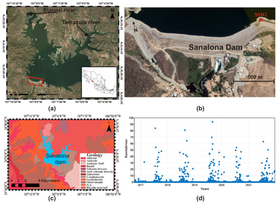
Figure 1.
Location of the Sanalona Dam (red rectangle) taken from Google Earth: (a) general location of the Sanalona Dam in the Tamazula and Sianori rivers; (b) detailed image of the crest of the Sanalona Dam. The red triangle is the location of the GPS station, SSIG; (c) geological setting of the Sanalona dam; (d) hydrological cycle of the study area. The blue dots represent the rainfall measurements in mm.
The Sanalona dam has a crest length and width of 1031 m and 10 m, respectively, a height of 81 m and a base of 415 m (see Figure 1b). It was the first dam to be built in the Sinaloa state region, triggering an economy in the Culiacan valley, where approximately 60,000 ha of farmland are currently irrigated with the help of the water contained by the Sanalona dam. In addition, the dam is about to turn 75 years in constant operation, exceeding its 50-year safety period of life recommended by CONAGUA.
The geological structure of the area under consideration is composed of andesite, rhyolite–acid tuff, basalt, and intermediate tuff from the Tertiary period, as well as alluvial and conglomerate from the Quaternary period, both belonging to the Cenozoic era. Figure 1c illustrates the geological configuration of the Sanalona dam. On the other hand, the rainy season in the region plays an essential role in filling the reservoir since it reaches its maximum capacity in a short time. The highest rainfall of the year is recorded in July, August, and September, as shown in Figure 1d.
3. Methodology
3.1. MT-InSAR Displacements
InSAR analysis was carried out using MT-InSAR measurements considering Sentinel-1 data. For that, all the available Sentinel-1A/B scenes until the end of 2021 were processed in order to derive the vertical and E–W horizontal displacements. In particular, the ascending track was composed of 152 SLC IW scenes (20 Sentinel-1A and 132 Sentinel-1B) from 14 October 2014 to 18 December 2021, with an incidence angle of 39.0486° and a ground sampling of 3.70 and 13.97 m, respectively, for the range and azimuth direction. This included 162 scenes (Sentinel-1A) composed the descending track, with an incidence angle of 39.4565° and a similar ground sampling to the ascending track.
The processing methodology was the classical PS-InSAR analysis using SARPROZ [30] software where a master image is selected for each track, and all the connections between this master and the rest of the images in the stack are computed. The master images were automatically selected by the software in the middle of the stacks, the image of 16 August 2016, for the ascending track and 9 January 2017, for the descending one. Once co-registering all the images with respect to the master scene, the reflectivity map is computed and a ground control point is selected for geocoding the results. Then, the Atmospheric Phase Screen (APS) is computed over a large area around the dam and removed from the final phase estimates. Finally, the PSs are obtained by deriving for each one the Line-of-Sight (LOS) displacements for each track. After the ascending and descending tracks are computed, both LOS displacements are combined to decompose the movements in the vertical and E–W velocities. First, the software computes possible shifts between the ascending/descending datasets estimating the offsets in longitude, latitude, and height. Precise offsets are then estimated using points with distances closer than the range specified as a maximum planar distance and with height differences closer than a maximum height distance. For processing the ascending/descending pairs, a maximum planar distance and maximum height distance are used, as well to identify the corresponding points in the two datasets. Once offsets have been estimated and ascending/descending pairs are identified (in the case of ascending and descending dataset pairs), the decomposed movement can be computed, plotted, and exported. Several options are available for that. For example, all points, ascending/descending pairs, or a grid created on overlapping areas can be generated.
To combine the LOS displacements of the ascending and descending mode, first, the PSs were identified on the crest of the Sanalona dam that corresponded to the same PSs but observed at different angles and from opposite directions (ascending and descending). Subsequently, it was necessary to establish the same evaluation period for each track, since the analysis period of the ascending mode begins and ends before the descending mode; for this, a timeline was defined for both modes, and the LOS data were interpolated every 12 days. In this way, the PSs located on the crest of the Sanalona dam in both modes contain the same period to be evaluated, from 5 October 2016 to 18 December 2021, every 12 days. On the other hand, due to the studied dam’s long service, its settlement process decreased decades ago. Therefore, the vertical displacements in the dam are insignificant. Consequently, the observed displacements are entirely attributed to horizontal displacements [2].
It is necessary to project the displacements from E–W to N–S. Subsequently, the N–S component must be rotated and converted into radial displacement, since the displacements caused by the thrust of the reservoir on the crest of the dam have a greater effect on the transversal component (radial displacement). Therefore, the mathematical model of the Sanalona dam was used to estimate the crest orientation and use this angle to extract radial displacements following the strategies proposed by Jänichen et al. [1]. Radial displacements are considered positive towards the downstream direction.
3.2. Finite Element Model of the Sanalona Dam
To obtain the structural response of the Sanalona Dam, the SAP2000 finite element software was implemented in the study [31]. In general, SAP2000 is a finite element software with an object-oriented 3D graphical interface, prepared to carry out, in an integrated way, the modeling, analysis, and dimensioning of the most comprehensive sets of structural engineering problems. SAP2000 is well-known for its capabilities to easily analyze structures and its visually friendly data interpretation. Moreover, this software is one of the most used by structural engineers around the world. The versatility in modeling structures allows its use in the dimensioning of bridges, buildings, stadiums, dams, industrial structures, maritime structures, and all types of infrastructure that need to be analyzed and dimensioned [31]. The geometric dimensions and the composition of the different materials of the Sanalona dam are illustrated in Figure 2.
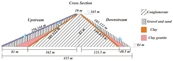
Figure 2.
Geometry of the cross-section of the Sanalona Dam.
Table 1 summarizes the mechanical and physical properties of the materials used in the finite element analysis performed by SAP2000. On the other hand, due to the computational complexity that a solid-based three-dimensional model would require, it was decided to model the cross-section of the Sanalona dam through plate-type (Shell-thick) elements. The model represents a unit strip (1 m) of the dam crest. Figure 3 shows the finite element model implemented in SAP2000 software. Each color of the model corresponds to a different type of material. In turn, the coordinate axis adopted for the analysis is indicated in Figure 3; “x” is the direction of interest when representing the deformation caused by the pushing force of the water, “Y” is the direction parallel to the height, and finally, “Z” is parallel to the longitudinal direction of the dam. Regarding the boundary conditions, the cross-section base was considered restricted to the displacements.

Table 1.
Mechanical and physical properties of the Sanalona dam materials. is the density, V is the Poisson ratio, E is the elastic modulus, is the angle of friction, and C is the cohesion.
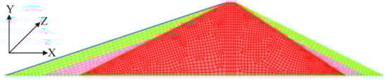
Figure 3.
Cross-section FEM model of the Sanalona dam.
3.3. GPS Displacements
3.3.1. Data Acquisition
A continuous-monitoring GPS station for seismic purposes was instrumented on the right-hand side of the Sanalona dam (see Figure 1b, red triangle tagged as SSIG). The GPS station is located approximately 670 m from the center of the crest, as can be seen in Figure 1b as well. The station comprises a TRM57971.00 antenna and a TRIMBLE NETRS receiver. It started operations on 24 June 2016 and is still working at present. The station is compatible only with the GPS constellation and has a sample rate of 1 Hz configured. Unfortunately, due to the remote access to the SSIG station, it is complex to solve technical problems, resulting in a data gap that may be present in the response time series. The binary files sampled at 1 Hz were shared by the National Seismological Service of Mexico (known as SSN in Mexico) corresponding to the measurement period from 24 June 2016 to 23 March 2022 and were converted to RINEX (Receiver INdependent EXchange) and decimated to 30 s with the help of TEQC software [32].
3.3.2. GPS Processing Strategies
The GPS observation files in RINEX 2.11 format corresponding to the evaluation period were processed in the CSRS-PPP service using the absolute precise point positioning (PPP) method in static mode. CSRS-PPP is a free online service developed and maintained by the Geodetic Survey Division of Natural Resources Canada [33]. The Canadian Spatial Reference System (CSRS) allows users to send their GPS observation files from a single receiver over the internet and achieve precise positioning. CSRS-PPP can process dual-frequency PPP solutions with GPS L1 and L2 and GLONASS L1 and L2 frequency bands. Integer ambiguity resolution is available for data collected on or after 1 January 2018. Data collected before this date will continue to be processed with the IGS final products without integer ambiguity resolution [34]. Additionally, Table 2 summarizes the processing parameters used by the CSRS-PPP service.
Table 2.
CSRS-PPP Service’s processing parameter summary.
The ECEF (XYZ) coordinates resulting from the processing were transformed to the NEU (North, East, Up) topocentric coordinate system since the ECEF coordinates cannot be applied to interpret horizontal and vertical displacements on the dam due to their origin [35]. On the other hand, the NEU coordinates were transformed to local coordinates of the dam using the methodology proposed in [2], where the dam’s crest represents the longitudinal axis and perpendicular to it, the transverse axis. The origin of the time series was obtained by subtracting the mean of the time series from each datum that makes it up.
3.4. Probability of Failure Calculation Considering Dam Sliding
The concept of probability of failure and the approaches to obtain it are maturing, and they are widely reported in the literature [36,37,38]. In general, the safety of structures is computed using deterministic approaches based on safety factors. However, since the risk depends on the uncertainty of load and resistance parameters of the structure under consideration, approaches based on safety factors may fail to convey the actual margin of safety. Therefore, more rational techniques must be used to explicitly compute the margin of safety considering uncertainties related to load and resistance variables. In this sense, since uncertainties in load and resistance variables must be considered in risk analysis, it may be hard to satisfy the basic design requirements during the evaluation. A basic case of risk analysis is illustrated in Figure 4. It can be observed that two variables are considered, one related to the demand on the system (e.g., loads acting in a structure, ) and the other related to the capacity of the system (e.g., the resistance of the structure, ). Both and are random variables. Thus, they are randomly characterized based on mean values ( and . ), standard deviations ( and ), and corresponding probability density functions [ and ]. The deterministic or nominal values of load and resistance are illustrated in Figure 4 as and , respectively. and are factors related to the safety that the structure is expected to have and depend on the structural system to be evaluated. Thus, the position of and , respectively, depends on the values of and . Therefore, the value of the probability of failure will also depend on the values and . In this context, if and are very large, then, will be small because and will be far apart. For example, in problems related to calculating the safety of critical structures, such as nuclear power plants, and are expected to be large.
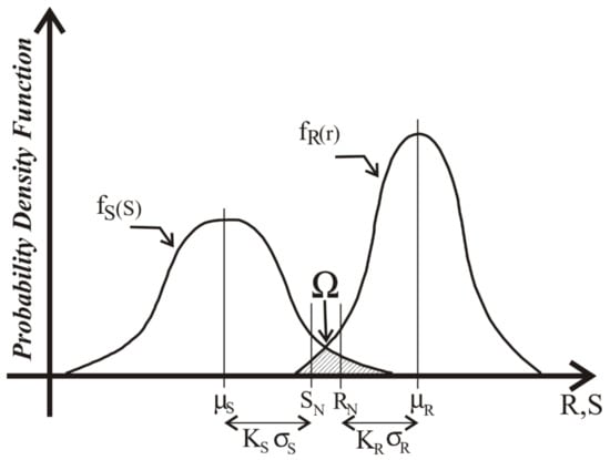
Figure 4.
Illustration of risk analysis of structures.
It is important to mention as well that the intent of conventional approaches can be explained by considering the overlapped or shaded area between both curves and as illustrated in Figure 4. The shaded/overlapped area presented in Figure 4 represents the probability of failure (pf), which depends on three factors of the two curves: the (1) relative position between them depending on the mean values ( and ), (2) dispersion among curves given by the standard deviations ( and ), and (3) shapes of the two curves represented by the corresponding Probability Density Function (PDF). Hence, deterministic design procedures achieve safety by selecting design variables in such a way that the overlapped area between and is kept minimum. Then, deterministic approaches generally shift the position of and using safety factors. Unfortunately, a more rational approach would be to calculate the underling risk by considering the above three factors (, and PDF). Thus, design variables would be selected satisfying an acceptable risk. To clarify this concept, the failure state of structural systems can be expressed as [29]:
where is the mathematical representation of the relationship of Random Variables (RVs).
The failure event or pf represents the shaded area () in Figure 4. It can be calculated by computing the overlapped area () between and as:
where is the joint PDF of the random variables related to resistance and load.
The integration of Equation (2) is performed over the failure region (). Generally, random variables related to and are a function of several other variables as gravity, lateral, and accidental loads and/or sectional and material properties. Hence, Equation (2) can be expressed in terms of multiple random variables as:
where is a vector that represents the load and resistance random variables (), and k is the total number of them.
Based on the above discussion, the limit state function can be defined as . This represents the boundary between the safe and unsafe region in the design parameter space, i.e., the state of a structure representing the limit between the appropriate and inappropriate performance. The limit state function and safe and unsafe regions are illustrated in Figure 5 in terms of and . The limit state function plays an important role in the calculation of reliability or risk. Combining Equations (2) and (3) and considering that failure occurs when , the pf can be calculated as:
where is the joint PDF related to the basic random variables represented by the vector .
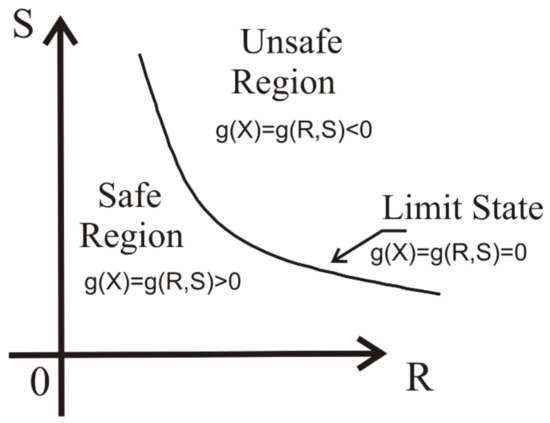
Figure 5.
Limit state concept.
The integration represented by Equation (4) is performed over the failure region []. If the random variables are statistically independent, the joint PDF can be replaced in Equation (4) by the product of individual PDFs. However, PDFs of random variables are difficult to obtain, and even if they were available, solving multiple integrals as presented in Equation (4) can be extremely complicated. Hence, an alternative is to use analytical approximations to solve the integral represented by Equation (4). Unfortunately, analytical approximations are often restricted to use only the mean () and coefficient of variation (VC) because the information about random variables may only be sufficient to evaluate and VC. As an alternative, the well-known Monte Carlo Simulation (MCS) can be implemented to solve it. In this sense, MCS can extract the probability of failure in the following way:
where is the estimate of the probability of failure, is the number of simulations where the failure occurred, and is the total number of simulations.
The Monte Carlo method requires a large enough number of simulations to find the desired value of . The limit state function was selected, established from the Mohr–Coulomb model. The Mohr–Coulomb criterion is used to evaluate the resistance to sliding of two rigid bodies in contact separated by a flat cemented layer. Based on this criterion, the sliding resistance fails when the sum of the intrinsic resistance of the intermediate layer plus the frictional resistance between the two contact surfaces is overpassed by the demands acting on the surface. If the normal stress () applied perpendicular to the contact plane increases, the shear strength () increases, as defined by a linear law that depends on a parameter known as the friction angle (). However, the intrinsic resistance (or cohesion, ) does not depend on the tension level, although it does depend on the properties and condition of the surface under consideration.
If is considered as the total normal force between bodies, is the cohesion and is the compressed length of the contact. The following expression may represent the Mohr–Coulomb criterion for the sliding stability of the Sanalona dam [4]:
where (reservoir thrust force) is the tangential destabilizing force parallel to the sliding plane, and is the internal friction angle, so that if is greater than the right-hand side of Equation (6), sliding will occur. In addition, in terms of structural safety, it must be stated that represents the resistance (R) and the load (S). Therefore, the limit state function that describes the performance of the dam, in terms of some essential random variables, is expressed as:
where is the area of the dam section in ; and are the density of the dam material and the density of the water in respectively; is the acceleration due to gravity in ; corresponds to the length of the base of the dam in ; is the height of the water in the reservoir in ; is the contact friction angle in degrees; and is the cohesion in contact in .
Analysis of Variables
Eight variables define the limit state function of the Sanalona Dam. They were presented in Equation (6). Based on previous studies, it was decided to consider only three of them as random variables. Random variables used in MCS are summarized in Table 3. These variables take commonly used distributions since certain information is available on the site of the Sanalona dam. On the other hand, considering the Mohr–Coulomb model, the shear strength parameters follow the normal distribution for the friction angle and the log-normal distribution for cohesion. For the selection of the probability distributions and parameters for each of the variables, we followed the publication of [4].
Table 3.
Selected random variables.
4. Results
This Section divides the results into three parts. First, the calculation of the radial displacements of the dam derived from the MT-InSAR technique is documented. Then, the simulated displacements coming from the FEM approach are reported. Afterwards, the measurements using GNSS GPS technology are presented. In addition, the analysis of the comparison between the reservoir level and the displacements is illustrated. Finally, the failure probability results for different reservoir levels are documented. In this sense, there are two main objectives of the following numerical analysis: (1) to measure the radial displacements of the dam with different methodologies, and (2) to extract the probability of failure of the dam using MCS.
4.1. Displacements
4.1.1. MT-InSAR Displacements
The Sanalona dam is located in a very vegetated area, which prevents the detection of many measurement points. Relatively few PSs were identified through both the ascending and descending processing, but their density was sufficient to sample the behavior of the dam crest using MT-InSAR. Figure 6 shows the mean LOS velocity maps for the ascending and descending processing together with the decomposed vertical and E–W mean velocity maps using a 5 × 5 m grid over the overlapping areas for a better visualization. Final displacements were estimated for 13 MT-InSAR PSs selected in the combined ascending and descending orbits along the Sanalona Dam. The location of the 13 PSs is presented in Figure 7. The ascending and descending LOS displacements were first combined and then converted into radial displacements, as explained in Section 3.1. The radial displacements for the 13 PSs follow a seasonal trend derived mainly from the reservoir filling at different times. Figure 8 illustrates the seasonal trend for point 148, located in the center of the crest, which presents the largest displacements, as expected due to its location. This trend is due to the beginning of the rainy season in the region, which is at the beginning of June and commonly reaches maximum displacements in November when the reservoir level is close to 100%. The radial displacements generally reach a maximum of up to 4 mm in November and decrease in the following months to −10 mm when the reservoir decreases in May. The PS located on the edges of the crest obey the behavior of the reservoir level but with maximum and minimum displacements lower than those obtained at the central points, within the precision range of the MT-InSAR technique.
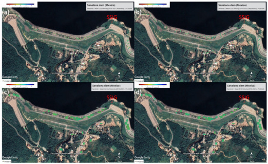
Figure 6.
Mean velocity maps for the MT-InSAR analysis of the Sanalona dam. (a) Ascending dataset in the LOS direction. (b) Descending dataset in the LOS direction. (c) Decomposed vertical direction. (d) Decomposed E–W direction.
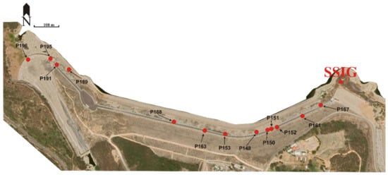
Figure 7.
Location of the 13 PSs identified along the Sanalona dam in the MT-InSAR analysis.
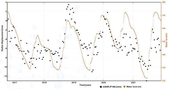
Figure 8.
Comparison between the radial displacements from MT-InSAR measurements at PS no. 148, located at the center of the crest, and the water level of the Sanalona dam.
On the other hand, the seasonal behavior of the displacements is correlated with the changes in the reservoir level, as seen in Figure 8. The radial displacements and the water level present a high similarity with a correlation index (r2) of 0.88. Therefore, it is shown that the water level is the main factor that generates the driving force of the deformation on the crest of the Sanalona dam.
4.1.2. FEM Displacements
The finite element analysis was carried out considering 100% of the capacity of the Sanalona dam (level of the spillway: 156.2 m). The pressure forces generated by the water were evaluated in terms of a triangular distribution of forces with respect to water depth. The forces were assigned to the model through distributed loads on the crest (rock layer element). Figure 9 illustrates the displacement contours of the model. In summary, it is observed that the displacements obtained in the crest width of the dam were 7.7 mm in the “X” direction and 0.7 mm in the “Y” direction.
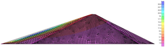
Figure 9.
Displacement contours in mm of the mathematical model of the Sanalona dam.
With the help of the finite element model of the Sanalona dam, it was possible to estimate the displacements produced by the pushing force of the water at different reservoir levels from 2016 to 2022. It was also possible to generate a regression model with a correlation of to calculate the displacements (“y”) from the reservoir level in meters (“x”). Equation (8) describes the regression model:
The radial displacements simulated by the FEM were determined using Equation (8) from the reservoir level for the evaluation period ranging from 5 October 2016 to 18 December 2022. Figure 10 represents the radial displacements obtained with the FEM and its relationship with the reservoir level. It is visible that these radial displacements presented the highest correlation with the reservoir level compared to GPS and MT-InSAR. The FEM modeling presented the highest correlation with the reservoir level. This last was considered a reference since the FEM represents, in a more detailed way, the structural performance of the dam. This is justified because FEM modeling considers the mechanical behavior of the materials that compose the dam when it is subjected to static and dynamic loads.
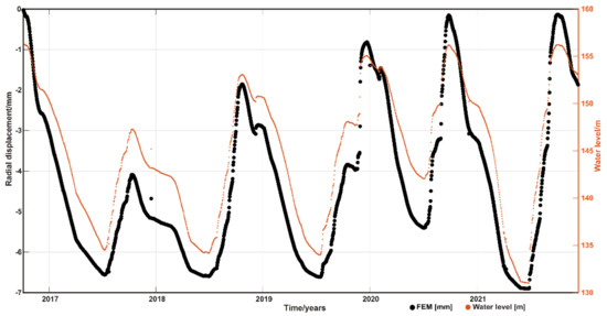
Figure 10.
Comparison of the simulated radial displacements with the mathematical model of the dam and the reservoir level.
4.1.3. GPS Displacements
The daily radial displacements of the Sanalona dam were extracted with the help of GPS observations by transforming them to local displacements of the structure. A low-pass digital filter commonly known as moving average with a 10-day window was applied to smooth the time series. This was performed with the objective of visualizing its long-term trend (See Figure 11). Once the low-pass filter was applied to the time series, they were shortened to the analysis period. Figure 11 shows a similar behavior between the reservoir level and the radial displacements measured with GPS. In addition, Figure 11 illustrates the deviation between the time series and the water level in the middle of the series. Thus, it is mainly due to the location of the SSIG station, which is not placed on the crest of the Sanalona dam (See Figure 1). However, the effects of the thrust force of the water are reflected in the zone of the SSIG station.
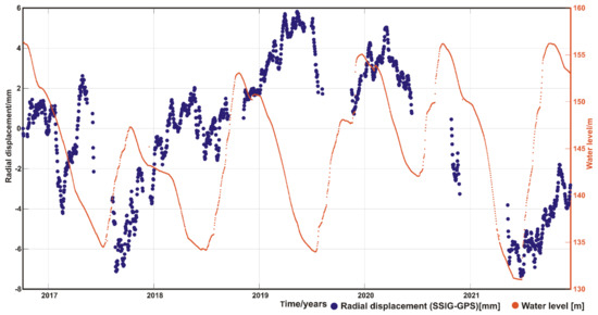
Figure 11.
Local radial displacements of the Sanalona dam through GPS measurements at the SSIG station.
It is observed in Figure 11 that the radial displacements of the area where the SSIG station is located increased in the rainy season due to the rise in the reservoir level of the dam. In this sense, the maximum deformation was on 12 May 2019, at 5.8 mm, which corresponds to the top level of the reservoir. When the reservoir decreases, the radial deformation also decreases; however, the minimum displacements are within the noise of the GPS measurements.
4.2. Accuracy Analysis of Radial Displacements
Considering the radial displacements obtained from the mathematical model of the Sanalona dam as the reference, the accuracy of the radial displacement measurements with MT-InSAR and GPS was analyzed. Figure 12 illustrates the displacements corresponding to over 5 years of four PSs. Due to the extensive vegetation in the area where the SSIG station is located, it was impossible to identify a nearby PS. Moreover, the radial displacements of GPS and FEM are observed and simulated, respectively, with the latter considered the reference. GPS observations were measured daily. However, there are certain gaps (lack of information) in the data that were not measured. MT-InSAR and FEM measurements have an observation frequency of 12 days. In this sense, the visual comparison among the three methods is visible in Figure 12.
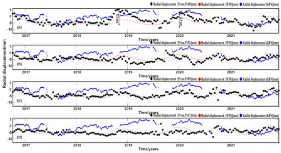
Figure 12.
Visual analysis of four InSAR (black dots) radial displacement zones and those obtained with GPS (blue line) and FEM (red dots). (a) PS no. P148 located in the central zone of the crest. (b) PS no. P152 situated in the center of the crest. (c) PS no. P189 located in the western zone of the crest. (d) PS no. P167 located in the eastern zone of the crest and close to the GPS station.
Figure 12a illustrates the radial displacements of PS no. P148, which is located in the central area of the Sanalona dam crest, where the greatest displacements are expected due to the thrust force of the reservoir. There are differences in magnitude in the time series of each methodology due to the errors of each one and the location of monitoring on the dam. PS no. P148 has better visual behavior than GPS when compared to FEM. This means that the observations on PS no. P148 from the ascending and descending satellites were highly precise at the acquisition time. The maximum displacements that PS no. P148 presents were in the order of 5 mm in one of the times when the reservoir is close to 100%. However, considering the origin of the displacements when the level of the reservoir is minimum, the maximum radial displacement that the crest has suffered corresponds to the year 2018 (see the first arrow in Figure 12a), reaching radial displacements of 12.4 mm during May (origin) and November (maximum). To determine the accuracy of the GPS and InSAR methods, it was necessary to generate Table 4, where the maximum displacements are observed for each reservoir level of 100% (or near) in the evaluated period. In the first three fills, the GPS and InSAR dam displacements obtained differences of less than 5 and 8 mm with respect to the FEM, respectively.
Table 4.
Maximum radial displacements at different filling times of the Sanalona dam.
The values of the GPS measurements have a time lag with respect to the InSAR and FEM measurements. This is because the radial displacements measured via InSAR and FEM presented a peak earlier, while the GPS values fall behind and showed a peak later. On the other hand, the displacements on PS no. P152 were lower, although it is located on the central zone of the crest as well. The maximum displacements recorded on PS no. P152 were 8.37 mm corresponding to 100% of the reservoir, as illustrated in Figure 12b. PS no. P189 is located towards the west of the dam, as illustrated in Figure 7. This PS has maximum displacements of 8.2 mm, caused mainly by the level of the reservoir, as seen in Figure 12c. On the other hand, PS no. P167, located on the eastern side of the crest and closest to the SSIG station, presented smaller radial displacements than the three previous PSs, with magnitudes of less than 5 mm. The seasonal trend of PS no. P167 does not follow a pattern similar to that of the FEM; that is, the radial displacements are little affected when the reservoir level is 100%. The reservoir level had less effect on PS no. P167 than GPS, even though they were in a similar area of the dam curtain with a separation of 115 m. The first half of the evaluation period of PS no. P167 presented variations of ± 2.5 mm, that is, the uncertainty range of InSAR, which is observed in Figure 12d. In summary, the push force of the water has a greater impact on the western part of the curtain than on the eastern one. This phenomenon can be derived from the location of the body of the dam to the total reservoir and the construction design. Consequently, the area where PS no. P167 is located can be considered stable, and these displacement values are used to measure the accuracy of the InSAR technique. InSAR is the best technique to evaluate the radial and vertical displacements in the dams caused by the reservoir level. It represents an alternative to high-precision leveling due to the precision achieved.
4.3. Probability of Failure by Sliding
For the calculation of the probability of failure by sliding of the Sanalona dam, six reservoir levels were identified, which represent the minimum level, average level, and maximum level of the reservoir, as well as the level of the spillway, the level of the crest, and a level above the crest (See Table 5). These levels are within the evaluation period. In this context, 100 million simulations were performed for each reservoir level using the MCS. Figure 13 illustrates the probability of failure obtained for each reservoir level.
Table 5.
Probability of failure for different reservoir levels.
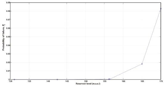
Figure 13.
Estimation of the probability of failure by sliding for different reservoir levels applying the Monte Carlo simulation method.
For the minimum reservoir level, is never reached out due to the low magnitude of the elevation of the stored water in the dam. Considering that the low levels of the reservoir correspond to lower load states than those with the high levels, the estimation of the probability of failure makes mathematical sense for this study. The minimum value of corresponds to the minimum level of the reservoir, and the maximum value of pf corresponds to the maximum level of the reservoir. When the reservoir levels are low, the is 0; that is, the structural safety of the Sanalona dam is high, and it does not present any risk to society and/or users. However, based on and according to the results of Table 4 and Figure 13, the reservoir levels equal to or above the level of the crest do represent a risk to the safety of the dam due to the high load demand.
5. Discussion
It is important to apply different measurement methodologies to consider a complete study of monitoring displacements on a dam. The MT-InSAR technique is used to study structures with slow and long-range movements, such as dams. On the other hand, one of the most common methods for the mathematical study of structures is the FEM approach since it allows a more detailed analysis of the structure and establishes its integrity. The most accurate satellite technology to measure specific displacements is GPS since it allows permanent monitoring of a structure regardless of environmental conditions. However, most of the reported studies of displacement on the dam crest were based on MT-InSAR and GPS; these approaches only report the magnitudes and the precision with which they were obtained. It is important to mention that SHM goes beyond just quantifying the magnitudes of different variables on a structure. Identifying the structural integrity of a dam based on risk analysis methodologies considering the quantification of the dam–reservoir system is one of the objectives of the SHM. In particular, in this study, the probability of failure for a system response is calculated for a given load event and the case of an earthfill dam.
To ensure precise monitoring with MT-InSAR, it is necessary to identify many PSs on the dam crest. However, the physical properties of the objects located near the crest, such as the variation in the vegetation during the year, means that some PSs are only observed from geometry. In this study, 13 common PSs were selected for the ascending and descending geometry over the crest of the Sanalona dam. For the processing, 152 scenes from the ascending geometry corresponding to 14 October 2014 to 18 December 2021 and 162 scenes for the descending geometry were used. The classical PS-InSAR processing methodology was used in the SARPROZ software. The LOS measurements of both geometries were spatially interpolated, and the vertical and horizontal E–W displacements were later estimated from the combination of satellite geometries. Horizontal displacements were converted to radial displacements using the dam crest azimuth. The 13 MT-InSAR PSs are distributed along the 1031 m of the concrete crest. The 13 common PSs presented displacements with different magnitudes, mainly those located in the center and outside the crest. The PS that presented the highest correlation with the reservoir level was PS no. P148, located in the center of the crest. The area where PS no. P148 is located presented a displacement of close to 13 mm in the filling from May to November 2018, when the dam reached 81% of the reservoir level. The displacements of the central area of the crest are caused by force generated by the level of the reservoir on the structure. On the other hand, the PSs located outside the central zone of the crest do not have a high correlation with the level of the reservoir. However, these areas also present radial displacements, but in periods when the reservoir level is low. Possibly, these alterations are due to variations in temperature and vegetation.
To evaluate the use of MT-InSAR technology in the structural monitoring of dams, it was necessary to make a comparison between the displacements obtained by this technique with those simulated by a FEM and those measured by the GPS technique. The displacements simulated by FEM obey a mathematical model created from the geometry and properties of the materials contained in the evaluated dam. Material properties can commonly be fitted to a probability density function with a history of in situ measurements. However, it is essential to know precisely the magnitudes of the physical properties of the materials because they are input parameters for the FEM and the calculation of the probability of failure. In the case of GPS measurements, these are affected by different sources of error that cause the studied phenomenon to be altered. It is important to consider theoretical models of corrections and precise products. For this study, the GPS continuous monitoring station was not instrumented for structural monitoring but for seismic studies of the region. Therefore, the station is located outside the central zone of the dam crest, where the displacements are fewer due to the little effect of the push force of the water on the structure. Therefore, the radial displacements measured with MT-InSAR and those simulated with FEM for the central area of the crest were not expected to be the same as those measured via GPS. Identifying a trend derived from the reservoir level in the three evaluated techniques was what was sought. The FEM is considered the reference technique due to its high correlation with the reservoir level ( 1). Therefore, the radial displacements measured with MT-InSAR in the evaluation period should have a similar behavior to those simulated with the FEM but with a different magnitude, due to the measurement principle of each technique. The PS no. P148, located in the central zone of the studied dam’s crest, registered the greatest radial displacements. When the reservoir level is minimal, the dam structure is not subjected to load; therefore, its body does not suffer deformations, and the dam is at repose. When the reservoir level increases due to the rainy season, the radial displacements increase until they reach a maximum due to the applied load in the crest. The effect of the load on the dam crest is visible in Figure 12a. The maximum radial displacement of the crest was 12.4 mm for the year 2018 and 11.9 for 2020. PS no. P152, located approximately 100 m from PS no. P148, presents the same trend, but a different magnitude in the displacements. PS no. P152 reached maximum magnitudes of displacements close to 9 mm. PS no. P189, located on the left side of the crest, showed greater radial displacements than those measured on PS no. P167, located at the other end of the crest (right side). The maximum radial displacements achieved on PS no. P189 and PS no. P167 were 8.2 mm and about 5 mm, respectively. These differences in the extreme zones of the crest are due to the design of the dam and the orientation it has regarding the total reservoir; therefore, the forces of the reservoir are distributed in an inhomogeneous way over the body of the Sanalona dam.
The radial displacements of PS no. P148 InSAR and the reservoir level presented a high similarity, with a correlation coefficient of 0.88, demonstrating the high precision of the InSAR technique in tracking movements over dams. Finally, the risk assessment of the dam–reservoir system through the calculation of the probability of failure shows that for a maximum historical level of the reservoir (101.5%), a is obtained, a probability that does not represent a structural risk for the dam. On the other hand, a simulation of a 151.2% reservoir is made, representing a water level 5 m above the curtain of the dam, possibly a phenomenon that will never happen. However, the risk to the structure is high due to the applied load and the slight resistance that the dam will oppose.
The radial displacements measured on the crest of the Sanalona dam with the InSAR technique presented high accuracy when compared with those simulated by the FEM, In [1], the authors analyze the radial displacements and compare them with those measured by a pendulum located in the center of the curtain of the Moehne dam, reaching displacements above 4 mm. On the other hand, the radial displacements in the Sanalona dam presented magnitudes greater than 10 mm, with magnitudes 4 times the uncertainty achieved by InSAR [39,40]. Additionally, in [6], the authors compared the PS-InSAR results with those obtained with GPS and found a similar behavior; that is, InSAR has the capacity to reach precisions similar to those of GPS. In general, in this investigation, the results achieved with InSAR were similar in precision to those published in other studies. Additionally, this article contains a risk assessment. It can be presented as one of the first studies where radial displacements on the crest of an earthfill dam are monitored with three different methods and giving it a probabilistic approach to extract the risk represented by the level of the reservoir on the structure of a dam.
6. Conclusions
In this study, two satellite geodesy techniques were applied to monitor the radial displacements of the Sanalona dam located in northwest Mexico and compare them with those simulated from the dam’s finite element model. Likewise, an analysis of the probability of failure by sliding for different reservoir levels was carried out. Maximum radial displacements of 12.4 mm were detected with InSAR, with 6.7 mm for FEM and 7.3 mm for GPS. The InSAR technique presented a seasonal trend similar to the reservoir level and a correlation close to 0.9. On the other hand, the behavior of the radial displacements simulated with the FEM and measured with InSAR presented a similar trend with differences in magnitude in the order of 5 mm. GPS presented a different trend due to the location of the station. The InSAR results showed that it is a good and precise technique for monitoring movements in earthfill dams. In addition, many InSAR points distributed over the dam curtain were identified, which represented a better understanding of the structural behavior of the dam when it is subjected to different levels of load caused by the reservoir. The central zone of the crest presented the greatest displacements and the extreme zones the least. Indeed, the radial displacements of the dam are mainly caused by the reservoir. When the reservoir level of the Sanalona dam reaches its maximum, the structural risk increases inversely, and when the reservoir level decreases due to the absence of rain, the risk of a possible failure of the dam–reservoir system is null. The results of the probability of failure represent the risk of a possible failure of the reservoir–dam system; therefore, based on the for a 100% reservoir, it does not represent a risk for society since the performance of the Sanalona dam, for such a case, would be similar to the risk presented for the original design.
Author Contributions
Conceptualization, J.R.V.-O., A.M.R.-A. and M.C.d.L.; methodology, J.R.V.-O., A.M.R.-A., M.C.d.L. and J.R.G.-C.; software, J.R.V.-O., A.M.R.-A., M.C.d.L., J.R.G.-C. and M.A.-D.; validation, J.R.V.-O., A.M.R.-A., M.C.d.L., J.R.G.-C. and M.A.-D.; formal analysis, J.R.V.-O., A.M.R.-A., M.C.d.L., J.R.G.-C. and M.A.-D.; investigation, J.R.V.-O., A.M.R.-A., M.C.d.L., J.R.G.-C. and G.E.V.-B.; data curation, J.R.V.-O., A.M.R.-A. and M.C.d.L.; writing—original draft preparation, J.R.V.-O., A.M.R.-A., M.C.d.L. and J.R.G.-C.; writing—review and editing, J.R.V.-O., A.M.R.-A., M.C.d.L., J.R.G.-C. and G.E.V.-B.; supervision, A.M.R.-A., M.C.d.L., J.R.G.-C. and G.E.V.-B.; project administration, A.M.R.-A. and M.C.d.L. All authors have read and agreed to the published version of the manuscript.
Funding
This research was funded by CUMex-AUIP 2022.
Data Availability Statement
Data can be made available on request.
Acknowledgments
Research was supported by SIAGUA project PID2021-128123OB-C21 and PID2021-128123OB-C22 (AEI/FEDER, UE), POAIUJA 2023-24, and CEACTEMA, from the University of Jaén (Spain), and the RNM-282 research group from the Junta de Andalucía (Spain). “The seismological data were obtained by the National Seismological Service in Mexico. We are grateful to SSN staff for station maintenance and the acquisition and distribution of data”.
Conflicts of Interest
The authors declare no conflict of interest.
References
- Jänichen, J.; Schmullius, C.; Baade, J.; Last, K.; Bettzieche, V.; Dubois, C. Monitoring of Radial Deformations of a Gravity Dam Using Sentinel-1 Persistent Scatterer Interferometry. Remote Sens. 2022, 14, 1112. [Google Scholar] [CrossRef]
- Vazquez-Ontiveros, J.R.; Martinez-Felix, C.A.; Vazquez-Becerra, G.E.; Gaxiola-Camacho, J.R.; Melgarejo-Morales, A.; Padilla-Velazco, J. Monitoring of local deformations and reservoir water level for a gravity type dam based on GPS observations. Adv. Space Res. 2022, 69, 319–330. [Google Scholar] [CrossRef]
- Alcay, S.; Yigit, C.O.; Inal, C.; Ceylan, A. Analysis of displacements response of the Ermenek dam monitoring by an integrated geodetic and pendulum system. Int. J. Civ. Eng. 2017, 16, 1279–1291. [Google Scholar] [CrossRef]
- Altarejos-Garcia, L. Contribution to the Estimation of the Probability of Failure of Concrete Gravity Dams in the Risk Analysis Context. Ph.D. Thesis, Universidad Politécnica de Valencia, Valencia, Spain, 2009. [Google Scholar]
- Altarejos-Garcia, L.; Escuder-Bueno, I.; Serrano-Lombillo, A.; Membrillera-Ortuño, M.G. Methodology for estimating the probability of failure by sliding in concrete gravity dams in the context of risk analysis. Struct. Saf. 2012, 36, 1–13. [Google Scholar] [CrossRef]
- Maltese, A.; Pipitone, C.; Dardanelli, G.; Capodici, F.; Muller, J.P. Toward a comprehensive dam monitoring: On-site and remote-retrieved forcing factors and resulting displacements (gnss and ps–insar). Remote Sens. 2021, 13, 1543. [Google Scholar] [CrossRef]
- Scaioni, M.; Marsella, M.; Crosetto, M.; Tornatore, V.; Wang, J. Geodetic and remote-sensing sensors for dam deformation monitoring. Sensors 2018, 18, 3682. [Google Scholar] [CrossRef]
- Pytharouli, S.I.; Stiros, S.C. Ladon dam (Greece) deformation and reservoir level fluctuations: Evidence for a causative relationship from the spectral analysis of a geodetic monitoring record. Eng. Struct. 2005, 27, 361–370. [Google Scholar] [CrossRef]
- Guler, G.; Kilic, H.; Hosbas, G.; Ozaydin, K. Evaluation of the Movements of the Dam Embankments by Means of Geodetic and Geotechnical Methods. J. Surv. Eng. 2006, 132, 31–39. [Google Scholar] [CrossRef]
- Casaca, J.; Braz, N.; Conde, V. Combined adjustment of angle and distance measurements in a dam monitoring network. Surv. Rev. 2015, 47, 181–184. [Google Scholar] [CrossRef]
- Barzagui, R.; Cazzaniga, N.E.; De Gaetani, C.I.; Pinto, L.; Tornatore, V. Estimation and comparing dam deformation using classical and gnss techniques. Sensors 2018, 18, 756. [Google Scholar] [CrossRef]
- De Lacy, M.C.; Ramos, M.I.; Gil, A.J.; Franco, O.D.; Herrera, A.M.; Aviles, M.; Dominguez, A.; Chica, J.C. Monitoring of vertical displacements by means high-precision geodetic levelling. Test case: The Arenoso dam (South of Spain). J. Appl. Geod. 2017, 11, 31–41. [Google Scholar] [CrossRef]
- Xi, R.; Zhou, X.; Jiang, W.; Chen, Q. Simultaneous estimation of dam displacements and reservoir level variation from GPS measurements. J. Int. Meas. Confed. 2018, 122, 247–256. [Google Scholar] [CrossRef]
- Yigit, C.O.; Alcay, S.; Ceylan, A. Displacement response of a concrete arch dam to seasonal temperature fluctuations and reservoir level rise during the first filling period: Evidence from geodetic data. Geomat. Nat. Hazards Risk 2016, 7, 1489–1505. [Google Scholar] [CrossRef]
- Acosta, L.E.; De lacy, M.C.; Ramos, M.I.; Cano, J.P.; Herrera, A.M.; Aviles, M.; Gil, A.J. Displacements study of an earth fill dam based on high precision geodetic monitoring and numerical modeling. Sensors 2018, 18, 1369. [Google Scholar] [CrossRef]
- Xiao, R.; Shi, H.; He, X.; Li, Z.; Jia, D.; Yang, Z. Deformation monitoring of reservoir dams using GNSS: An aplication to south-to-north water diversion proyect, China. IEEE Access 2019, 7, 54981–54992. [Google Scholar] [CrossRef]
- Reguzzoni, M.; Rossi, L.; Gaetani, C.L.; Caldera, S.; Barzaghi, R. GNSS-based dam monitoring: The application of a statistical approach for time series analysis to a case study. Appl. Sci. 2022, 12, 9981. [Google Scholar] [CrossRef]
- Montillet, J.-P.; Szeliga, W.M.; Melbourne, T.I.; Flake, R.M.; Schrock, G. Critical infrastrcture monitoring with global navigation satellite systems. J. Surv. Eng. 2016, 142, 4016014. [Google Scholar] [CrossRef]
- Zhang, S.; Chen, B.; Gong, H.; Lei, K.; Shi, M.; Zhou, C. Three-dimensional surface displacement of the eastern beijing plain, china, using ascending and descending sentinel-1a/b images and levelling data. Remote Sens. 2021, 13, 2809. [Google Scholar] [CrossRef]
- Macias-Valadez, D.; Santerre, R.; Larochelle, S.; Landry, R. Improving vertical GPS precision with a GPS-over fiber architecture and real-time relative delay calibration. GPS Solut. 2012, 16, 449–462. [Google Scholar] [CrossRef]
- Guilhot, D.; Martinez del Hoyo, T.; Bartoli, A.; Ramakrishnan, P.; Leemans, G.; Houtepen, M.; Salzer, J.; Metzger, J.S.; Maknavicius, G. Internet-of-things-based geotechnical monitoring boosted by satellite insar data. Remote Sens. 2021, 13, 2757. [Google Scholar] [CrossRef]
- Qu, C.; Qiao, X.; Shan, X.; Zhao, D.; Zhao, L.; Gong, W.; Li, Y. InSAR 3-D coseismic displacement field of the 2015 Mw 7.8 Nepal earthquake: Insights into complex fault kinematics during the event. Remote Sens. 2020, 12, 3982. [Google Scholar] [CrossRef]
- Pawluszek-Filipiak, K.; Borkowski, A. Monitoring mining-induced subsidence by integrating differential radar interferometry and persistent scatterer techniques. Eur. J. Remote Sens. 2021, 54, 18–30. [Google Scholar] [CrossRef]
- Ruiz-Armenteros, A.M.; Marchamalo-Sacrsitán, M.; Bakon, M.; Lamas-Fernández, F.; Delgado, J.M.; Sánchez-Ballesteros, J.P.; González-Rodrigo, B.; Lazecky, M.; Perissin, D.; Sousa, J.J. Monitoring of an embankment dam in southern Spain based on Sentinel-1 time-series InSAR. Procedia Comput. Sci. 2021, 181, 353–359. [Google Scholar] [CrossRef]
- Xiao, R.; He, X. Deformation monitoring of reservoirs and dam using time-series InSAR. Geo. Inf. Sci. Wuhan Univer. 2019, 44, 1334–1341. [Google Scholar] [CrossRef]
- Tomas, R.; Cano, M.; Garcia-Barba, J.; Vicente, F.; Herrera, G.; Lopez-Sanchez, J.M.; Mallorqui, J.J. Monitoring an earthfill dam using differential SAR interferometry: La Pedrera dam, Alicante, Spain. Eng. Geol. 2013, 157, 21–32. [Google Scholar] [CrossRef]
- Milillo, P.; Perissin, D.; Salzer, J.T.; Lundgren, P.; Lcava, G.; Milillo, G.; Serio, C. Monitoring dam structural health from space: Insights from novel InSAR techniques and multi-parametric modeling applied to the pertusillo dam basilicata, Italy. Int. J. Earth Obs. Geoinf. 2016, 52, 221–229. [Google Scholar] [CrossRef]
- Maierhifer, C.; Reinhard, H.W.; Dobmann, G. Non-Destructive Evaluation of Reinforced Concrete Structural; Woodhead Publishing CRC Press: Cambridge, UK, 2010. [Google Scholar]
- Hariri-Ardebili, M.A. Risk, Reliability, Resilience (R3) and deyond in dam engineering: A state-of-the-art review. Int. J. Dis. Risk Reduct. 2018, 31, 806–831. [Google Scholar] [CrossRef]
- Perissin, D. Sarproz Software Manual. 2009. Available online: https://www.sarproz.com/software-manual/ (accessed on 1 November 2022).
- CSI. SAP2000 Integrated Software for Structural Analysis and Design; Computers and Structures Inc: Berkeley, CA, USA, 2013. [Google Scholar]
- Estey, L.H.; Meertens, C.M. TEQC: The Multi-Purpose Toolkit for GPS/GLONASS Data. GPS Solut. 1999, 3, 42–49. [Google Scholar] [CrossRef]
- CSRS-PPP. Canadian Spatial Reference System Precise Point Positioning. 2022. Available online: https://webapp.csrs-scrs.nrcan-rncan.gc.ca/geod/tools-outils/ppp.php?locale=en (accessed on 8 October 2022).
- Banville, S. CSRS-PPP Version 3: Tutorial. 2020. Available online: https://webapp.csrs-scrs.nrcan-rncan.gc.ca/geod/tools-outils/sample_doc_filesV3/NRCanCSRS-PPP-v3_TutorialEN.pdf (accessed on 8 October 2022).
- Yigit, C.O. Experimental assessment of post-processed kinematic Precise Point Positioning method for structural health monitoring. Geomat. Nat. Hazards Risk. 2016, 7, 360–383. [Google Scholar] [CrossRef]
- Gaxiola-Camacho, J.R.; Azizsoltani, F.J.; Villegas-Mercado, F.J.; Haldar, A. A novel reliability technique for implementation of Performance-Based Seismic Design of structures. Eng. Struct. 2017, 142, 137–147. [Google Scholar] [CrossRef]
- Haldar, A.; Mahadevan, S. Probability, Realibility and Statistical Methods in Engineering Design; Wiley: New York, NY, USA, 2000. [Google Scholar]
- Melchers, R.E.; Beck, A.T. Structural Reliability Analysis and Prediction, 3rd ed.; Wiley: New York, NY, USA, 2018. [Google Scholar]
- Selvakumaran, S.; Plank, S.; GeiB, C.; Rossi, C.; Middleton, C. Remote monitoring to predict bridge scour failure using Interferometric Synthetic Aperture Radar (InSAR) stacking techniques. Int. J. Appl. Earth Obs. Geoinf. 2018, 73, 463–470. [Google Scholar] [CrossRef]
- Milillo, P.; Giardina, G.; Perissin, D.; Milillo, G.; Coletta, A.; Terranova, C. Pre-collapse space geodetic observations of critical infrastructure: The morandi bridge, genoa, italy. Remote Sens. 2019, 11, 1403. [Google Scholar] [CrossRef]
Disclaimer/Publisher’s Note: The statements, opinions and data contained in all publications are solely those of the individual author(s) and contributor(s) and not of MDPI and/or the editor(s). MDPI and/or the editor(s) disclaim responsibility for any injury to people or property resulting from any ideas, methods, instructions or products referred to in the content. |
© 2023 by the authors. Licensee MDPI, Basel, Switzerland. This article is an open access article distributed under the terms and conditions of the Creative Commons Attribution (CC BY) license (https://creativecommons.org/licenses/by/4.0/).