Some Key Issues on Pseudorange-Based Point Positioning with GPS, BDS-3, and Galileo Observations

Abstract

Nowadays, BDS-3 and Galileo are still developing and have global service capabilities. This study aims to provide a comprehensive analysis of pseudorange-based/single point positioning (SPP) among GPS, BDS-3, and Galileo on a global scale. First, the positioning accuracy distribution of adding IGSO and GEO to the MEO of BDS-3 is analyzed. The results show that after adding IGSO and GEO, the accuracy of 3D in the Asia-Pacific region is significantly improved. Then, the positioning accuracy of the single-system and single-frequency SPP was validated and compared. The experimental results showed that the median RMS values for the GPS, Galileo, and BDS-3 are 1.10/1.10/1.30 m and 2.57/2.69/2.71 m in the horizontal and vertical components, respectively. For the horizontal component, the GPS and Galileo had better positioning accuracy in the middle- and high-latitude regions, while BDS-3 had better positioning accuracy in the Asia-Pacific region. For the vertical component, poorer positioning accuracy could be seen near the North Pole and the equator for all three systems. Meanwhile, in comparison with the single-system and single-frequency SPP, the contribution of adding pseudorange observations from the other satellite system and frequency band was analyzed fully. Overall, the positioning accuracy can be improved to varying degrees. Due to the observation of noise amplification, the positioning errors derived from dual-frequency SPP were much noisier than those from single-frequency SPP. Moreover, the positioning performance of single-frequency SPP with the ionosphere delay corrected with CODE final (COD), rapid (COR), 1-day predicted (C1P), and 2-day predicted (C2P) global ionospheric map (GIM) products was investigated. The results showed that SPP with COD had the best positioning accuracy, SPP with COR ranked second, while C1P and C2P were comparable and slightly worse than SPP with COR. SPP with GIM products demonstrated a better positioning accuracy than that of the single- and dual-frequency SPP. The stability and variability of the inter-system biases (ISBs) derived from the single-frequency and dual-frequency SPP were compared and analyzed, demonstrating that they were stable in a short time. The differences in ISBs among different receivers with single-frequency SPP are smaller than that of dual-frequency SPP.

1. Introduction

With the fast development of the global navigation satellite system (GNSS), GNSS has been widely used in the military, disaster prevention and mitigation, engineering construction, transportation, and urban management, and can provide positioning, navigation, and timing services with different levels of accuracy [1,2,3,4,5,6]. Pseudorange-based/single point positioning (SPP), as one of the most basic modes of GNSS, is used by users in various fields for its computational power, low cost, and fast positioning. The first one that can be used for SPP is the GPS. First of all, only the GPS is capable of SPP, and due to the influence of multiple error sources, the positioning accuracy of GPS SPP has an error of tens of meters [7]. Therefore, some researchers worked on improving the C/A code measurement accuracy and the signal-in-space ranging error (SISRE) of the broadcast ephemeris and improved the accuracy of both of them to 0.3 m and 0.7 m, respectively [8]. At present, the positioning accuracy of GPS SPP in horizontal and vertical components is limited to 1–2 m and 2–3 m, respectively [9]. Galileo had four available satellites in orbit in 2012 and was able to solve SPP independently. In recent years, Galileo satellites have been increasing, and there are now 30 satellites in orbit, with a positioning accuracy of 2–3 m for Galileo SPP in the horizontal component and different frequencies in the vertical component (2–3 m for E1 and 5–7 m for E5a, E5b, and E5 (ab)) [10]. Currently, BDS-3 has 30 satellites providing navigation, positioning, and timing services, including 24 medium earth orbit (MEO), 3 inclined geosynchronous satellite orbit (IGSO), and 3 geosynchronous earth orbit (GEO) satellites [11,12]. BDS SPP, using only the B1 frequency, can provide a positioning accuracy within 10 meters [13]. The positioning accuracy of single-frequency BDS SPP is better than 2 m and 5 m in horizontal and vertical components, respectively, if group delay and code deviation correction are incorporated into the error correction [14]. In addition, the estimated TEC noise proxies (for elevations higher than 60 deg.)—a 100 s root mean square (RMS) of TEC—were: 0.05 TECU for the Galileo E5 AltBOC, 0.09 TECU for the GPS L5, 0.1 TECU for the Galileo E5a/E5b BPSK, and 0.85 TECU for the Galileo E1 CBOC. Dual-frequency combinations provide RMS values of 0.03 TECU for the Galileo E1E5 and 0.03/0.07 TECU for the GPS L1L2/L1L5. At low elevations, E5 AltBOC provides at least twice as little single-frequency TEC noise as compared with the data obtained from E5a or E5b [15].

Since the data accuracy of broadcast ephemeris itself is poor, far below the accuracy of precision ephemeris and precision clock error products, and SPP is based on the data provided by broadcast ephemeris to calculate the satellite 3D position and satellite clock error, the positioning accuracy of SPP is limited to the level of meters [16]. To improve the positioning accuracy of SPP, some GNSS researchers have contributed to the research on improving mathematical models, error model correction, and accuracy improvement for GNSS broadcast ephemeris products. Firstly, regarding the mathematical model, a weighted least squares method based on least squares, with the satellite altitude cut-off angle as the weight, has remarkably improved the positioning accuracy. In addition, iterative least squares with the user-equivalent range error (UERE) as the weight, enhances the positioning accuracy of single-frequency SPP of four single systems, GPS, GLONASS, BDS, and Galileo, to 1/3/1.5/1.5 m, 1.5/3/1.5/1.5 m, and 2.5/6/ 2.5/3 m in E, N, and U components [17,18]. In terms of the error correction model, the effect of ionospheric delay is an essential error source for single-frequency SPP. Meanwhile, single-frequency receivers can only weaken the impact of ionospheric delay by various models. The commonly used ionospheric correction model is Klobuchar, which is widely used because of its simple algorithm [19]. Some researchers have improved the basic Klobuchar model and have developed the GPS Klobuchar model (GPSK8) and the BDS Klobuchar model (BDSK8), which are able to eliminate 64.8% and 65.4% of the ionospheric delay, respectively [20]. Except for the K8 model, some scholars have studied the BDS Global Broadcast Ionospheric Delay Correction Model (BDGIM), under which the global 3D positioning accuracy of BDS SPP can reach 3.5 m, which is better than the BDSK8 model in the mid-latitude region of the Northern hemisphere [21,22]. In addition, the accuracy of the predicted GIMs generated by three different IAACs (CODE, UPC, and ESA) has been evaluated. It was found that the accuracy of the predicted GIMs from CODE was better than that of the predicted GIMs from UPC and ESA, providing a reference for single-frequency GNSS [23].

Although the positioning accuracy of SPP has improved in the case of various mathematical models and error model corrections, the available satellites for a single system have been drastically reduced in areas with complex environments and severe occlusions, where the positioning accuracy is poor or even impossible. In order to obtain the positioning performance of SPP under different environments, the positioning performance of single GPS SPP under 10°, 20°, 30° and 40° satellite cut-off angles is solved by simulating different environments with different satellite cut-off angles. The results show that when the satellite altitude angle reaches more than 30 degrees, the number of GPS satellites decreases from 7 to 4, the PDOP value increases from about 3 to more than 6, and the 3D accuracy decreases from about 2 m to more than 4 m [24]. Therefore, some scholars have conducted multi-system combination SPP. The first multi-system combination was the GPS and GLONASS combination, which increased the number of available satellites and provided more stable positioning results in complex areas [25]. With the development of Galileo and BDS, the study of the combination of GPS and Galileo or BDS has also received attention [26]. When the GPS and four Galileo In-Orbit Validation (IOV) satellites are used for simultaneous positioning, the results are improved by 2% and 10% in the horizontal and vertical components, respectively [27]. The combination of GPS and BDS was first studied in the Australian region, where the combination of BDS and GPS can produce better positioning accuracy and position stability in areas with few available GPS satellites [28]. In the Asia-Pacific region, the combination of GPS and BDS-2 has dramatically improved the positioning accuracy by about 10% better than the case of GPS-only. The combination of multiple systems SPP not only improves the accuracy of navigation and positioning but also improves the integrity of positioning [29]. However, since different navigation and positioning systems have different time and coordinate bases, and the hardware delays between systems are receiver-dependent, all these factors may lead to systematic bias when making observations. Therefore, the time, coordinate base, and receiver hardware delay must be considered when performing multi-system fusion positioning [30]. This is the inter-system bias (ISB), and this error must be dealt with when performing multi-system SPP [31]. Calculating the ISB of the GPS and Galileo is easier because the GPS and Galileo have the same frequency (e.g., L1/L5 for the GPS and E1/E5a for Galileo). The ISB of the GPS and Galileo is discussed, and it is found that the value of ISB depends on the receiver type and can be up to hundreds of seconds, according to the data provided by The Cooperative Network for GIOVE Observation (CONGO) [32]. The effect of ISB must also be considered when performing the combined GPS and BDS SPP. The intra-day stability of the ISB of the GPS and BDS was evaluated using a hypothesis testing method. The result proves that ISB is stable in a short time and can be used as an a priori value [33].

In the last two decades, numerous scholars have studied the status accuracy of single-system SPP, but there are fewer studies on the positioning excellence of different systems within different regions. Meanwhile, some scholars have studied multi-system SPP, but there are fewer studies on the combination of BDS-3 and Galileo, while there are fewer studies on the addition of other systems to the current system in different regions. Based on the above, this paper first analyzes the status of three satellite systems, GPS, BDS-3, and Galileo, regarding the number of available satellites and PDOP. The following three single systems, GPS, BDS-3, and Galileo, are solved for single-frequency SPP at an elevation cut-off of 7°, respectively, to analyze the global distribution of the positioning accuracy in horizontal and vertical components and to compare the accuracy of the three systems. Additionally, we analyzed the dual-frequency single-system SPP. The gain of the combination of GPS with BDS-3 or Galileo, BDS-3 with GPS or Galileo, and Galileo with GPS or BDS-3 in relation to the single system was then examined. Meanwhile, using several ionospheric products, we evaluated the SPP’s accuracy. Finally, the stability and variability of ISB are explored.

2. Methodology of SPP

2.1. Pseudorange Observation Equations

For a specific satellite-receiver link, the general equations of pseudorange observations $P$ can be described as:

$$P_{r,j}^s={\rho }_r^s+c\left[\left(\delta t_r+d_{r,j}\right)-\left(\delta t^s+d_j^s\right)\right]+T_r^s+I_{r,j}^s+{\epsilon }_{r,j}^s$$

(1)

where $s$, $r$, and $j$ denote the satellite, receiver, and frequency band; ${\rho }_r^s$ represents the geometric distance; $\delta t_r$ and $\delta t^s$ are the receiver and satellite clock offsets; $c$ is the speed of light in vacuum; $T_r^s$ is the slant tropospheric delay along the direction from satellite $s$ to receiver $r$; $I_{r,j}^s$ is the slant ionospheric delay; $d_{r,j}$ and $d_j^s$ denote the receiver- and satellite-specific pseudorange hardware delays/biases; ${\epsilon }_{r,j}^s$ represents the unmodelled errors, such as the pseudorange observation noise and multipath effect, etc. It is noteworthy that $\delta t_r$ and $d_{r,j}$ are high-correlated, and so are $\delta t^s$ and $d_j^s$.

In SPP processing, the satellite position and clock offsets are calculated with broadcast ephemeris in advance. The tropospheric delays are corrected with empirical models, i.e., Saastamoinen. For single-frequency SPP, the ionospheric delays are also modeled with empirical models, such as the Klobuchar model for GPS, the BDGIM model for BDS-3, and the Nequick-G model for Galileo. For dual-frequency SPP, the ionospheric delays are usually eliminated by ionospheric-free (IF) combined observables. The corrections of the satellite-specific pseudorange hardware delays for single- and dual-frequency SPP can refer to the Interface Control Document of the specific satellite system.

2.2. Single-Frequency SPP

By taking the pseudorange observation on the first frequency as an example, the linearization of Equation (1) can be written as:

$$p_{r,1}^s={\mathit{g}}_r^s\cdot \mathit{x}+c\delta {\overline{t}}_r+{\epsilon }_{r,1}^s$$

(2)

where $p_{r,1}^s$ is observed, minus the computed value of the pseudorange observation; ${\mathit{g}}_r^s$ is the unit vector of the component from the receiver to the satellite; $\mathit{x}$ is the vector of the receiver position increments relative to the a priori position; $\delta {\overline{t}}_r$ is the reparameterized receiver clock offset that absorbs the receiver-specific pseudorange hardware delay, and $\delta {\overline{t}}_r=\delta t_r+d_{r,1}$.

2.3. Dual-Frequency SPP

For dual-frequency SPP, the linearized IF combined pseudorange observables are actually formed as:

$$p_{r,\mathrm{I}\mathrm{F}}^s={\mathit{g}}_r^s\cdot \mathit{x}+c\delta {\tilde{t}}_r+{\epsilon }_{r,\mathrm{I}\mathrm{F}}^s$$

(3)

with

$$\{\begin{array}{l}{p}_{r,\mathrm{I}\mathrm{F}}^s=\alpha \cdot p_{r,1}^s+\beta \cdot p_{r,2}^s\\ \delta {\tilde{t}}_r=\delta t_r+(\alpha \cdot d_{r,1}+\beta \cdot d_{r,2})\\ {\epsilon }_{r,\mathrm{I}\mathrm{F}}^s=\alpha \cdot {\epsilon }_{r,1}^s+\beta \cdot {\epsilon }_{r,2}^s\end{array}$$

(4)

2.4. The Handling of Receiver Clock Offsets in Multi-GNSS SPP

There are two schemes for the handling of receiver clock offsets in multi-GNSS SPP. The first method is that an independent receiver clock offset per GNSS is introduced. The second one only estimates the GPS-specific receiver clock offset, while for the other satellite system, the inter-system bias (ISB) is employed. In fact, the receiver clock offset for the other system is the sum of the GPS-specific receiver clock offset and ISB. Both methods are equivalent. In this study, the first method is adopted.

3. Data Sets and Processing Strategies

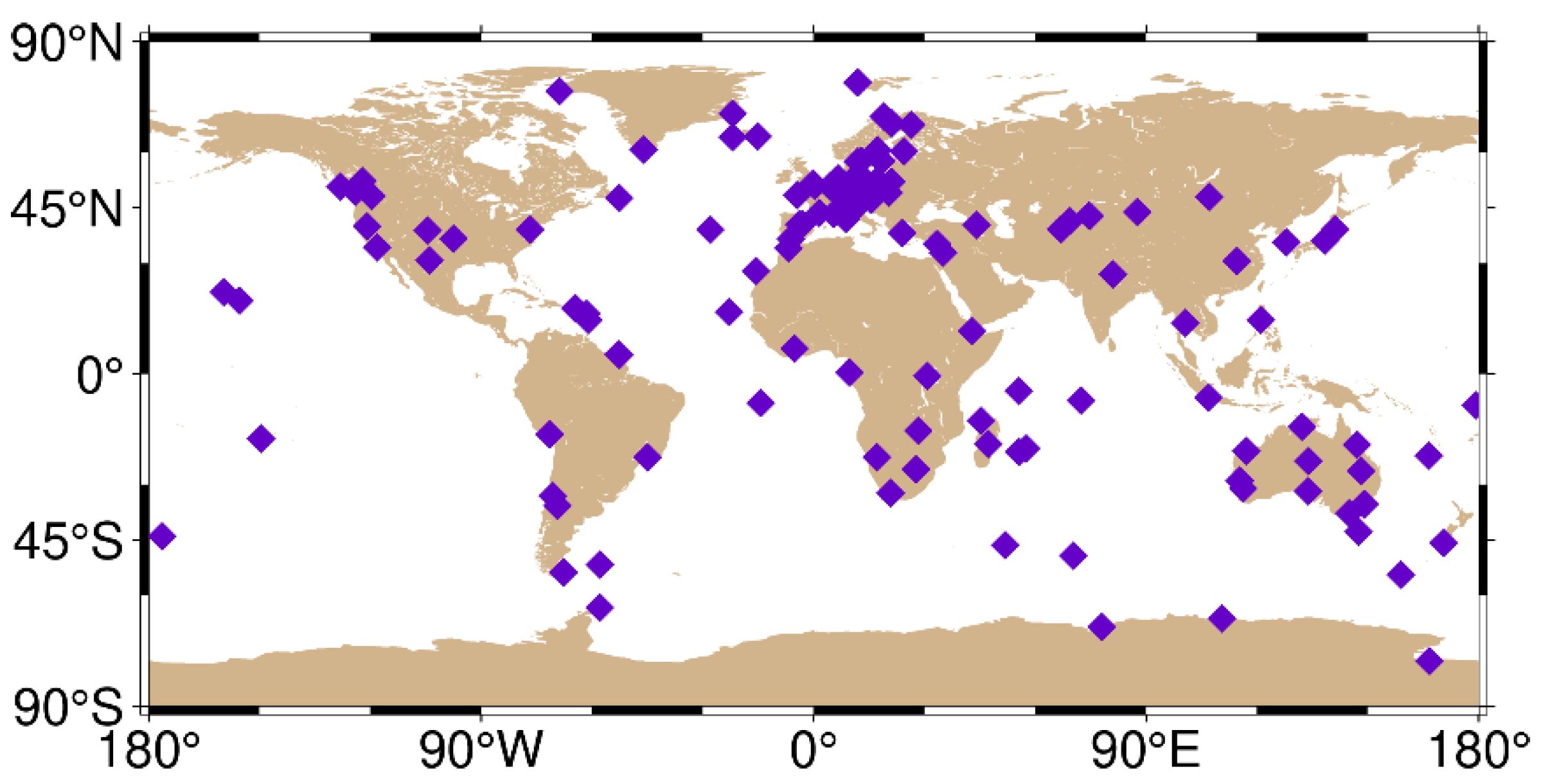
3.1. Data

In this paper, the observation files of 145 MGEX tracking stations with a sampling interval of 30 s for a total of 28 days from 1 February 2022 to 28 February 2022 (See: ftps://gdc.cddis.eosdis.nasa.gov/pub/gnss/data/daily accessed on 27 November 2022), and the broadcast ephemeris files provided by IGS (See: ftps://gdc.cddis.eosdis.nasa.gov/pub/gnss/data/daily/2022/brdc accessed on 2 June 2022) were selected for the solution. Figure 1 displays the geographical distribution of 145 tracking stations equipped with geodetic-type receivers, all of which can receive dual-frequency observations from three navigation satellites, namely GPS (L1/L2), BDS-3 (B1/B3), and Galileo (E1/E5a). The SPP was solved by using the open-source GAMP software, and the IGS SINEX weekly solution was used as the reference coordinates [34]. The specific processing strategies are provided in

Table 1. The strategy of SPP processing.

Items	Strategies
Number of tracking stations	145
Number of satellites	GPS(32), BDS-3(30), Galileo(30)
Signal selection	GPS(L1, L2), BDS-3(B1, B3), Galileo(E1, E5a)
Sampling rate	30 s
Satellite elevation cut-off	7°
Weight of observation value	Prior standard deviation of measurement error
Tropospheric delay	Saastamoinen delay model
Ionospheric delay	Single frequency and IF combination

.

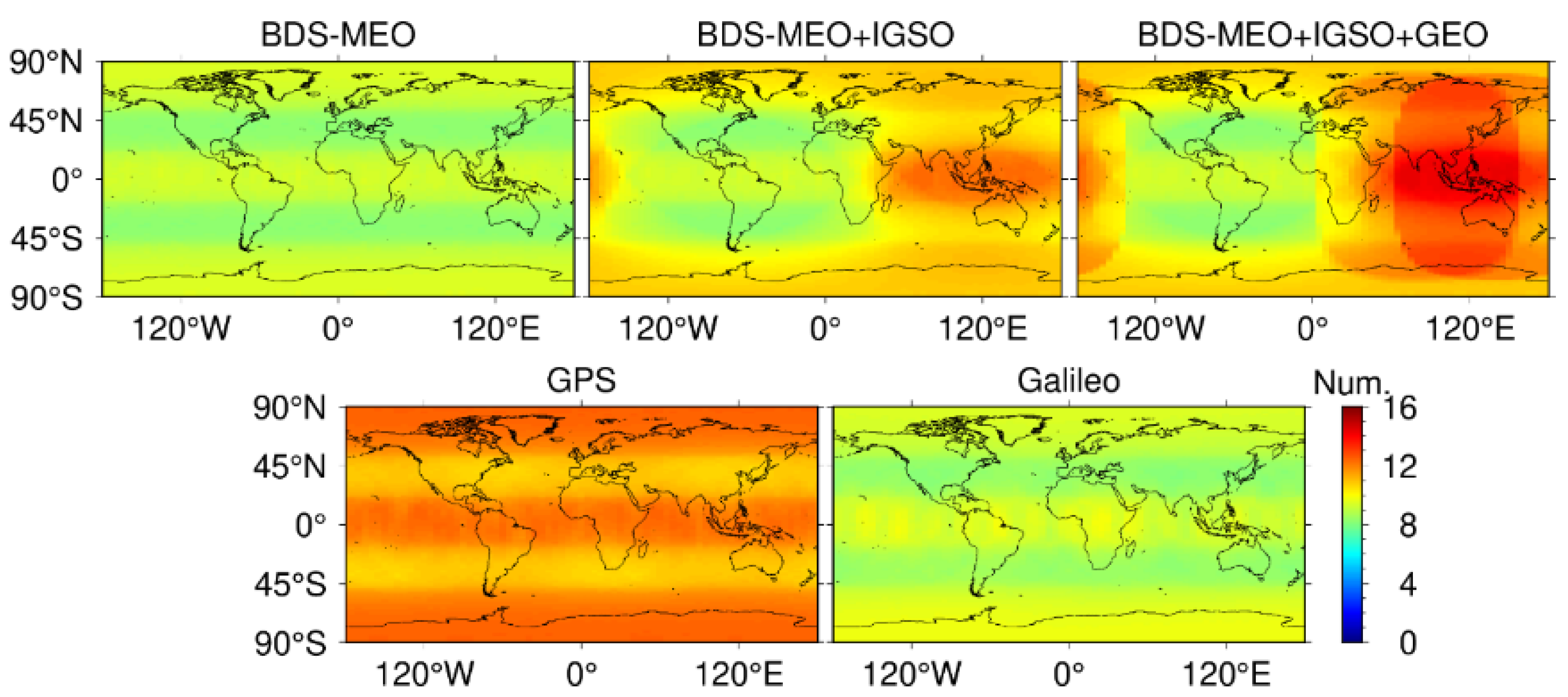
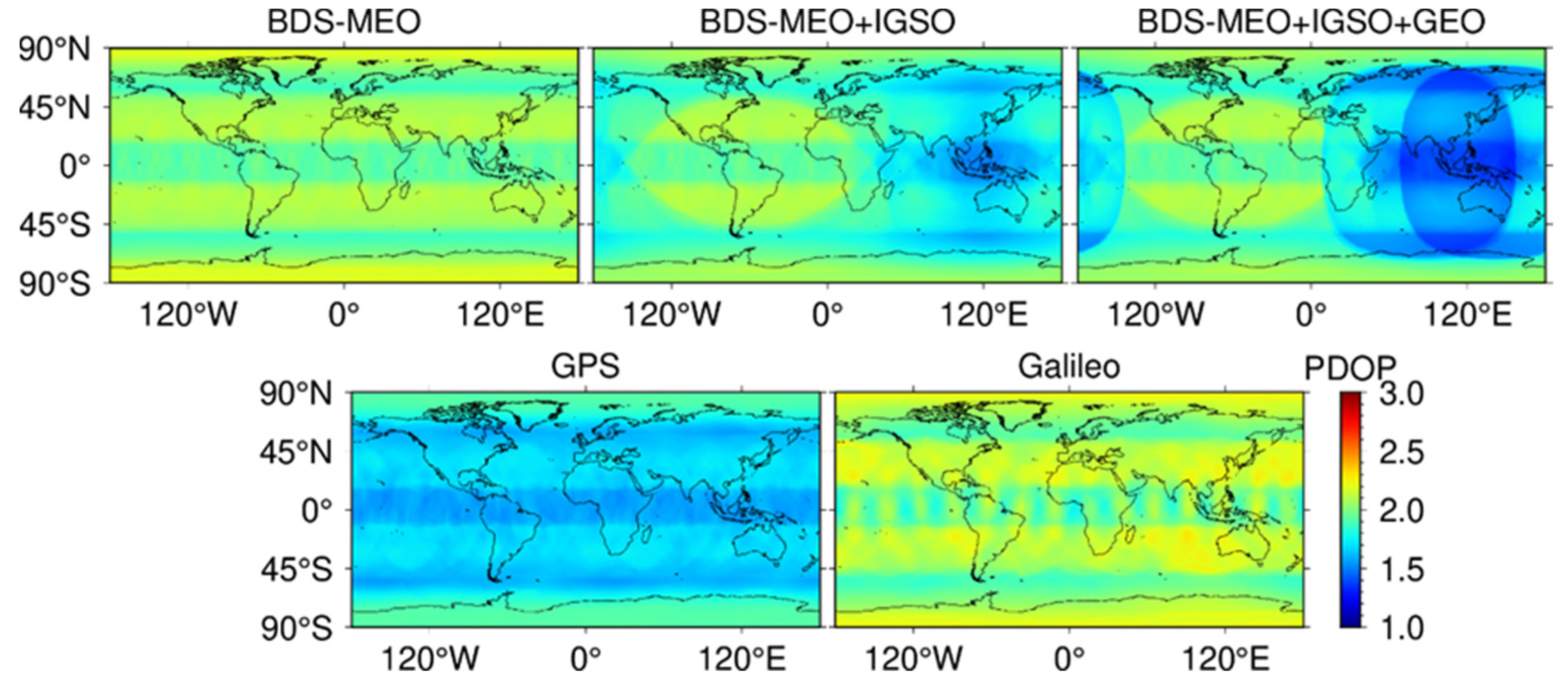
3.2. Availability Analysis of GNSS Constellations

This subsection mainly analyzes the number of visible satellites and position dilution of precision (PDOP) values for the GPS, Galileo, BDS-3-MEO, BDS-3-MEO+IGSO, and BDS-3-MEO+IGSO+GEO in any global location. Through a hypothetical simulation, we divide the world into 72 × 90 grids with 5° longitude and 2° latitude and assume that there is a receiver that can receive data from the GPS, BDS-3, and Galileo in the center of each grid [35]. The satellite cut-off elevation angle of the receiver is set to 7°, and the geodetic height is set to 100 m. In addition, whether a satellite can be used for positioning depends on the geometric relationship between the satellite and the receiver. This is because the satellite position accuracy calculated by the broadcast ephemeris and precision ephemeris differs by meter level, and the precision ephemeris provided by GFZ includes not only all available GPS and Galileo satellite data but also data from three types of BDS-3 satellites (MEO, IGSO, and GEO). Therefore, this paper calculates the satellite position using the precision ephemeris, with a sampling interval of 5 minutes, provided by GFZ.

Figure 2 displays the average number of visible satellites at different locations worldwide for the GPS, Galileo, BDS-3-MEO, BDS-3-MEO+IGSO, and BDS-3-MEO+IGSO+GEO on DOY 32 of 2022. The figure instructions consider that the GPS and Galileo have more visible satellites near the equator and at the poles, while fewer satellites are available in the mid-latitudes. In the case of GPS-only, there are 10–11 visible satellites at 20°–50°S and 20°–50°N and 12–13 visible satellites at other latitudes. The number of visible satellites for Galileo reached 10 in the low- and high-latitude regions. However, it is reduced to 8–9 at mid-latitudes. Since BDS-3 has three different orbits of satellites, the number of available satellites in the global region varies not only in latitude but also in the Eastern and Western hemispheres. For MEO alone, the number of visible satellites increases after an initial decrease from the low latitudes to the high latitudes, similar to the GPS and Galileo systems, with visible satellites at about eight at 20°–50°S and 20°–50°N, and about nine at other latitude regions. The visible satellites of BDS-3 will be strongly enhanced by the addition of GEO and IGSO. When IGSO is added, the number of visible satellites increases to 10–11 at high latitudes and 12 near the equator in the Eastern hemisphere, while when GEO is added, the number of visible satellites in the range of 40–180 E will increase dramatically. The number will reach 14 in the lower latitudes of the Eastern hemisphere. Thus, BDS-3 can better serve the Asia-Pacific region.

Figure 3 presents the global average PDOP values for the single-system situation for one day on 1 February 2022. The GPS has an average PDOP of 1.5–1.7 at the latitudes of 10°N–10°S, 40°–60°N, and 40°–60°S, and 1.7–1.9 at other latitudes. For Galileo, the average PDOP is 1.9–2.0 at 15°N–15°S, 50°–70°N, and 50°–70°S, and 2.0–2.3 at other latitudes. In the BDS-3-MEO case, similar to the GPS and Galileo, the PDOP increases from 1.9 to 2.1 and then decreases to 1.9 between 70°S and 70°N and is 2.0–2.2 at high latitudes. When the IGSO and GEO satellites are inserted, the DPOP in the Eastern hemisphere decreases dramatically between the longitudes 60° and 160°E. The PDOP ranged from 1.4 to 1.8 and even dropped to 1.3 near the equator.

4. Results Validation and Discussion

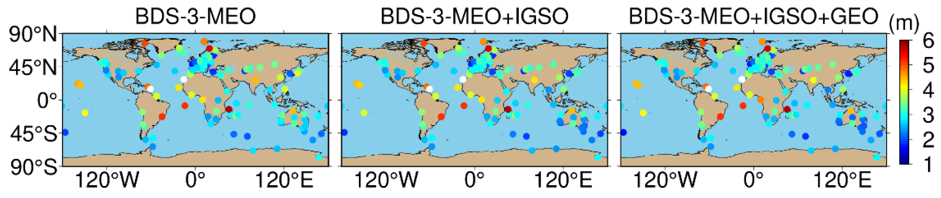
4.1. The Impact of Adding MEO, IGSO, and GEO Satellites for BDS-3 SPP

The orbital trajectories of the three satellite types of BDS-3 result in different positioning accuracies at different locations. Figure 4 shows that after adding IGSO to MEO, the positioning accuracy of the stations distributed in the Asia-Pacific region is significantly improved, and the RMS of 3D is increased from 3–4 m to 2.5–3 m. Adding GEO to MEO and IGSO, the accuracy improvement is not obvious.

Table 2. The number of accuracy improvements of adding IGSO in MEO and GEO in MEO and IGSO.

Satellite Type Added	Number Of Stations with Gain	Number of Stations with Reduced
MEO+IGSO	50	53
MEO+IGSO+GEO	40	30

lists the accuracy gains and decreases of 145 stations with IGSO in MEO and GEO in MEO and IGSO. Adding IGSO to MEO increases the accuracy by 4.7%, and adding GEO to MEO and IGSO increases the accuracy by 3.6%.

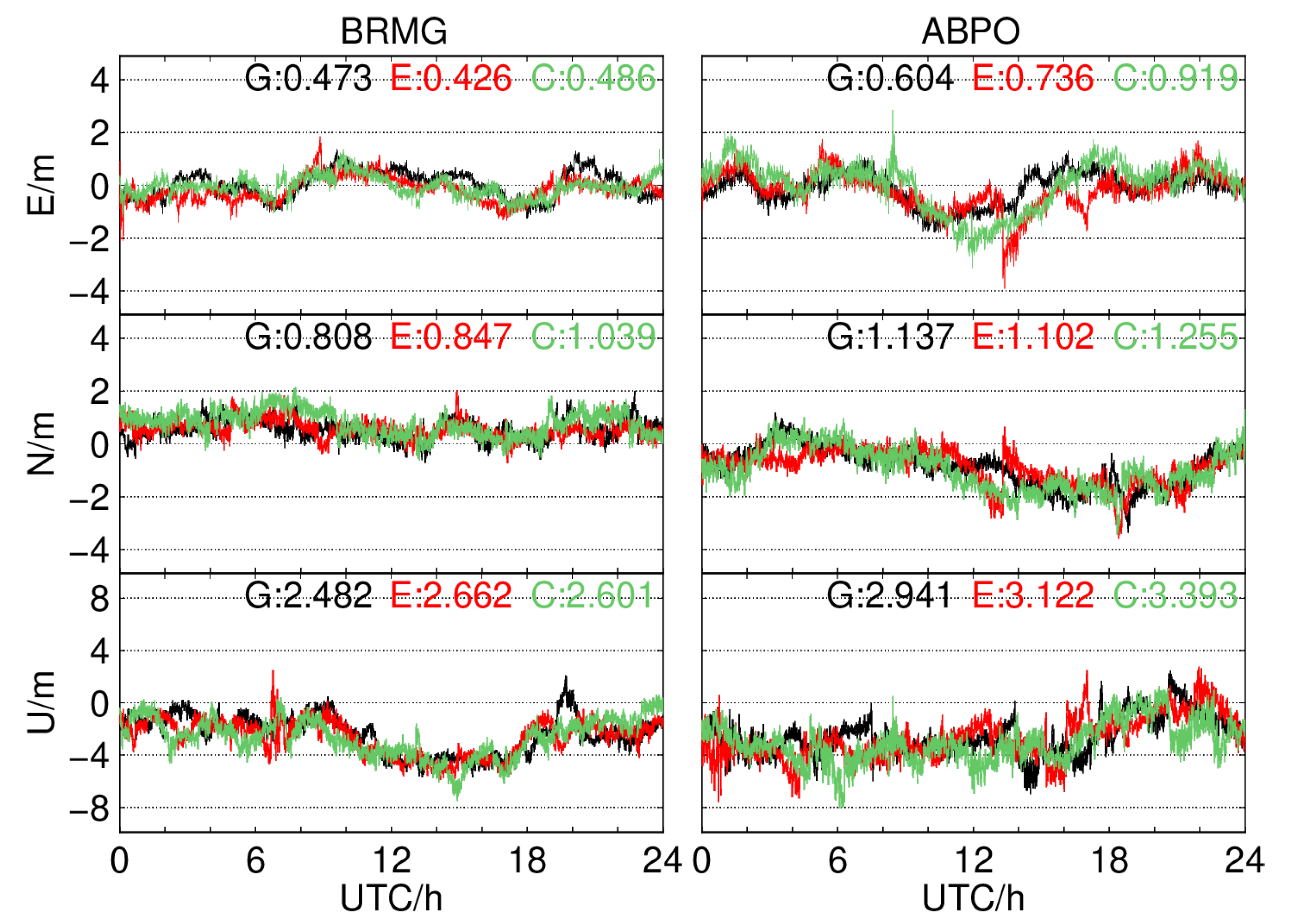
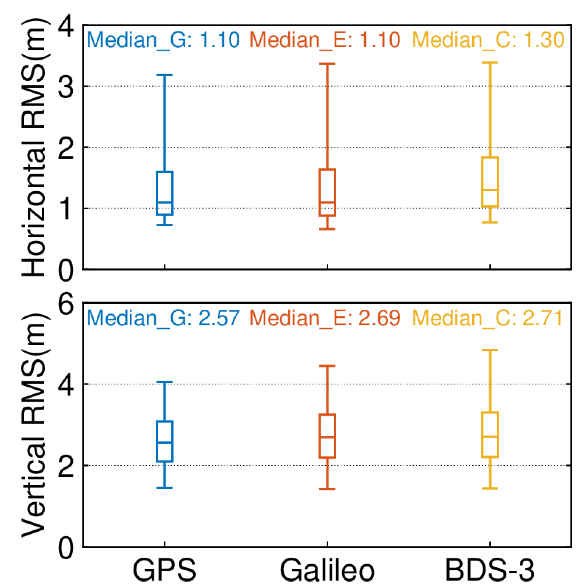
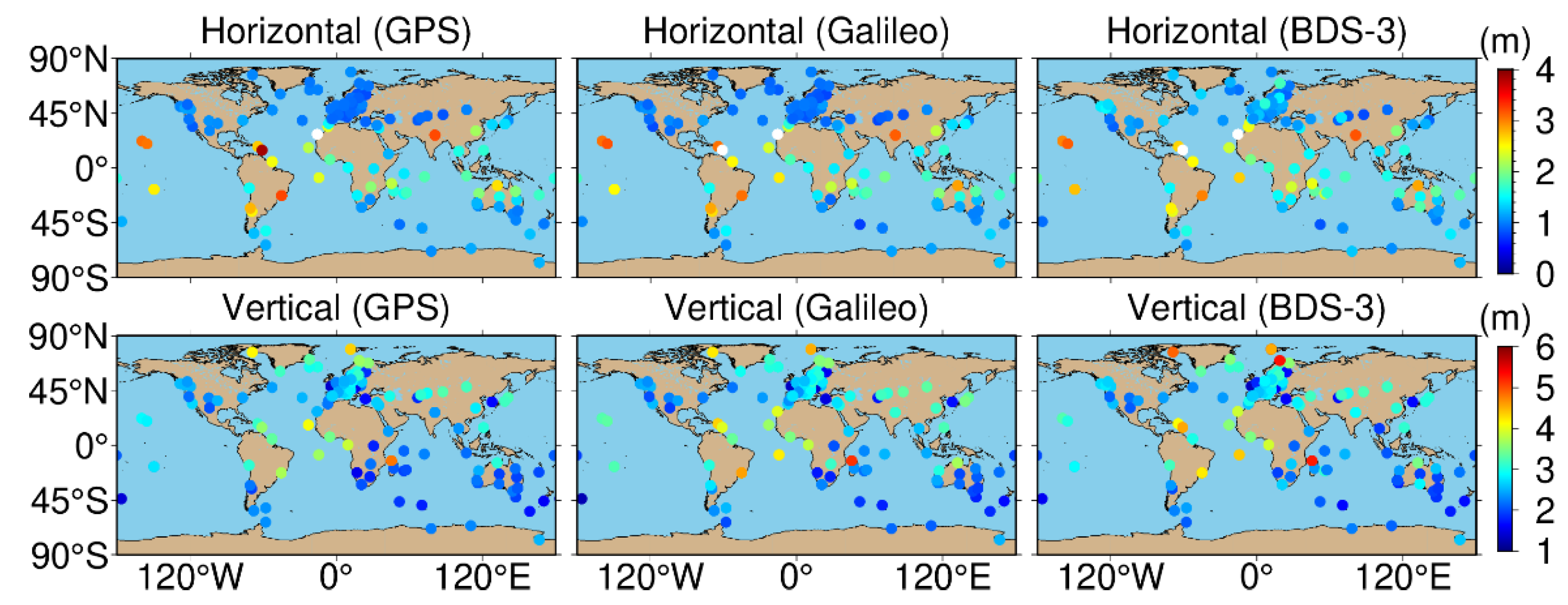
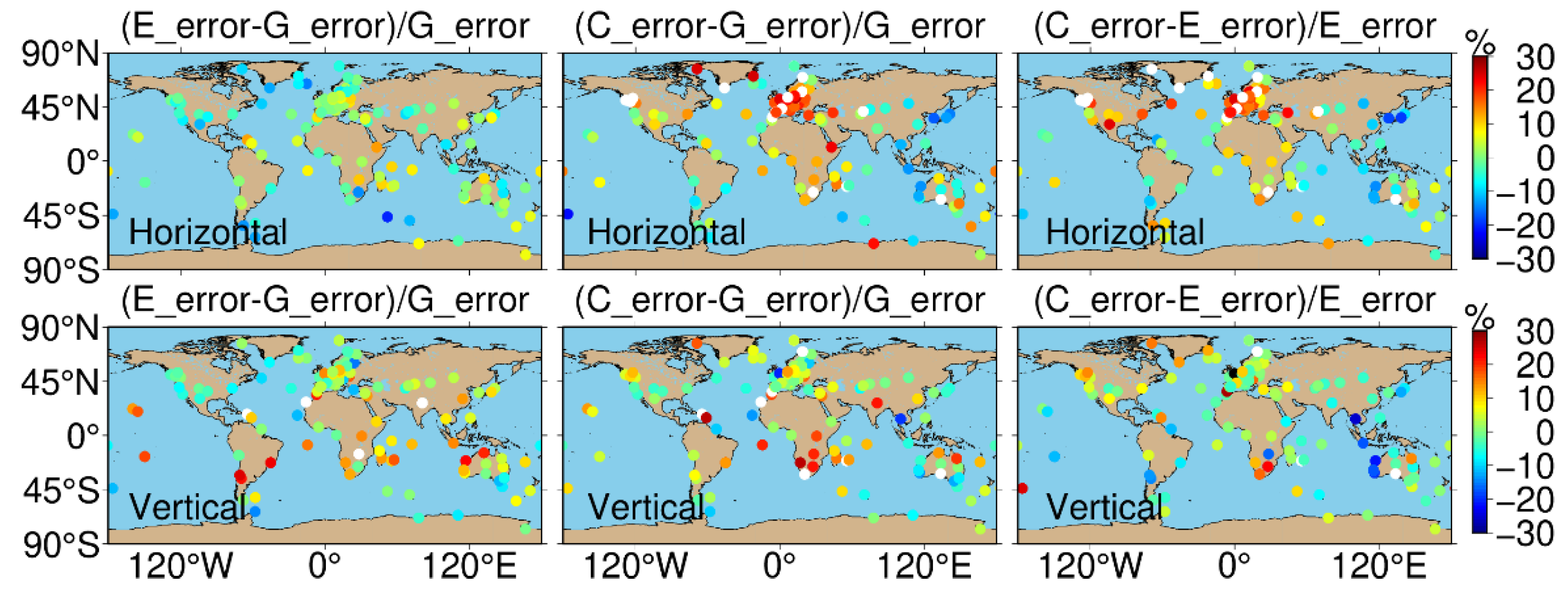
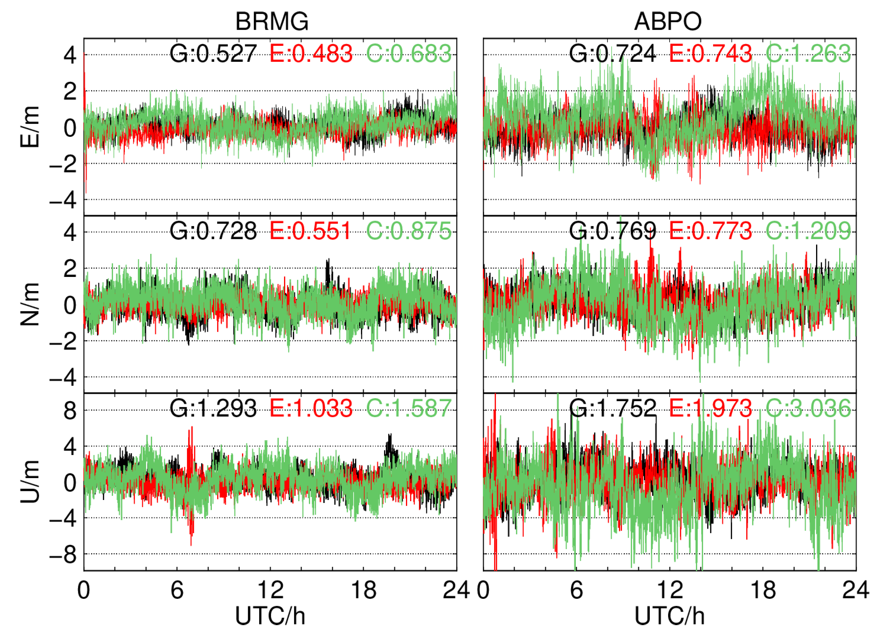
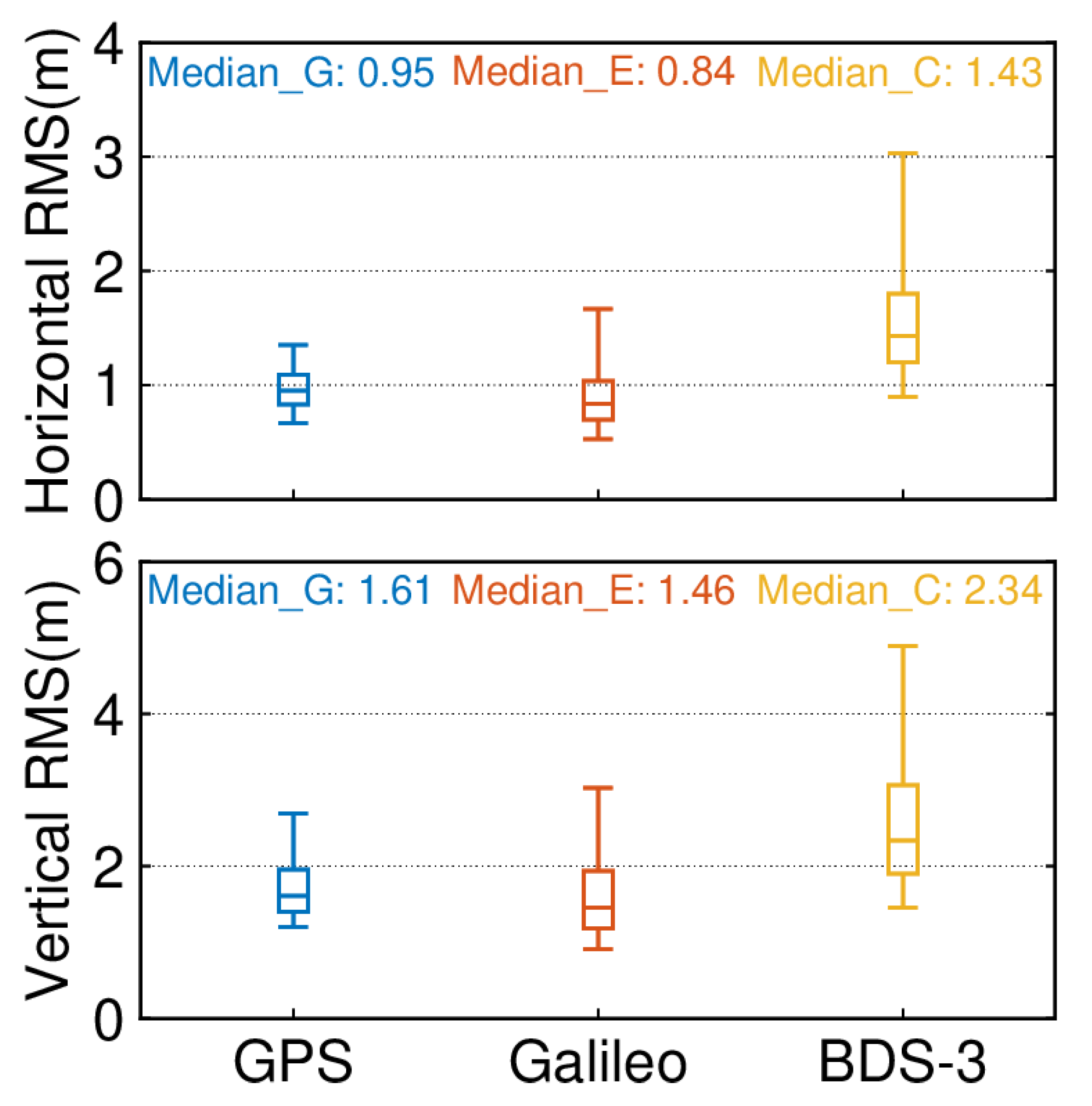
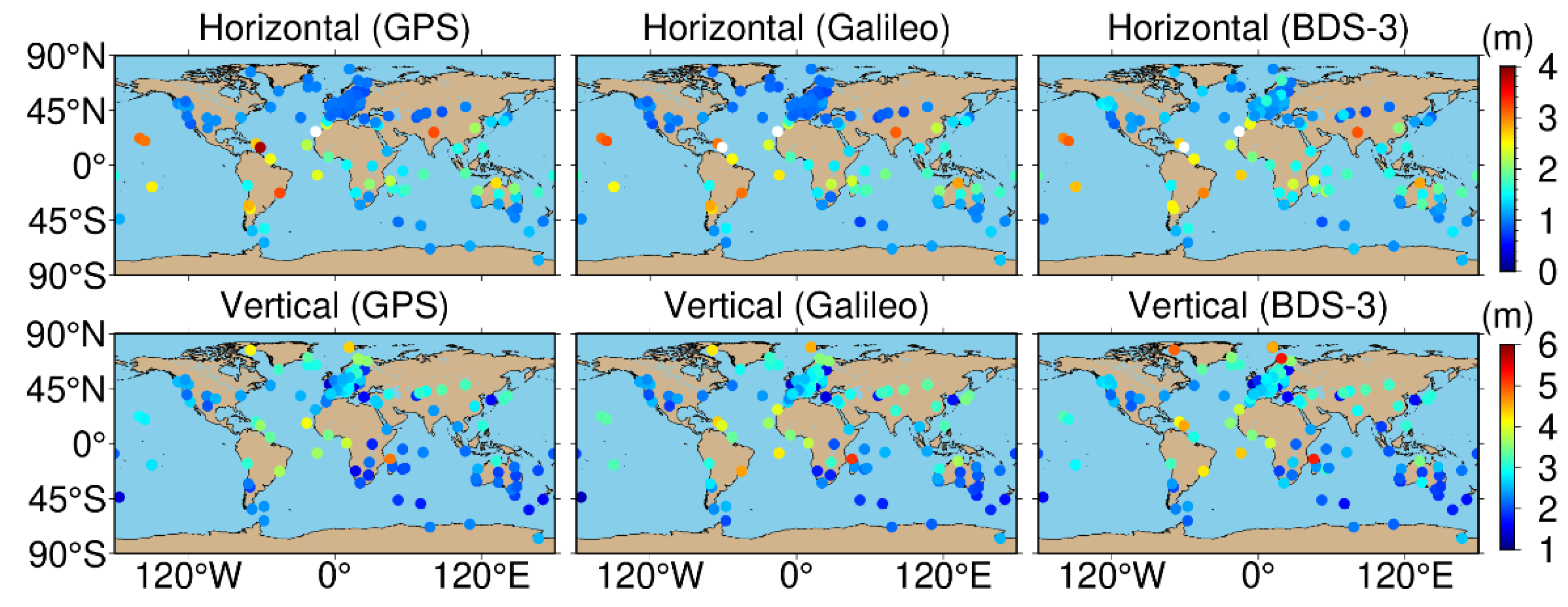
4.2. Single-System and Single-Frequency SPP (G, C, E)

This section primarily examines the positioning performance of single-frequency single systems (G, C, and E). We first selected the BRMG in the Southern hemisphere and the ABPO tracking station in the Northern hemisphere for SPP. Figure 5 shows the single-frequency positioning errors for 2880 epochs for each station. The error varies with roughly the same trend within 1 day for all three systems, and they all have varying levels of systematic error. In addition, the error values of the GPS and Galileo are relatively close, while the error of BDS-3 fluctuates more.

Figure 6 shows the number of visible satellites and PDOP values for the three systems during one day for the BRMG and ABPO tracking stations. Both stations are able to observe 7–11 GPS satellites and 5–9 Galileo satellites. BRMG is able to observe 7–19 BDS-3 satellites, while ABPO is able to observe 8–12 satellites. The PDOP values are between 2 and 3.

We then analyzed the overall positioning accuracy of the 145 tracking stations. Figure 7 presents the quartiles of the positioning errors (5%, 25%, 50%, 75%, and 95%) for the three single systems with an elevation cut-off of 7°. In the horizontal component, the median RMS of GPS-only and Galileo-only are the same, both at 1.10 m. The median RMS of BDS-3-only is larger than that of GPS-only and Galileo-only, at 1.30 m. In the vertical component, the GPS-only solution is the best, Galileo-only is the second best, and BDS-3-only is the worst. The median RMS of all three of them is 2.57/2.69/2.71 m. In both components, the 95% quantile RMS of the single system is less than 3.5 and 5 m.

Figure 8 exhibits the geographical distribution of the positioning accuracy for the 145 tracking stations of GPS, Galileo, and BDS-3, where white means exceeding the highest value of the ribbon, and black means less than the lowest value of the ribbon [36]. As shown in the figure, the geographic distribution of positioning accuracy is approximately the same for GPS-only and Galileo-only due to the similar distribution of the number of visible satellites around the world for these two systems. In the horizontal component, there is a significant difference in latitude between the GPS and Galileo tracking station accuracy distributions. The stations located at the middle and high latitudes in North America and Europe have a root mean square (RMS) value of about 1–1.2 m, but the RMS value increases to about 2 m for the tracking stations in the areas between 30° and 30°S and even reaches more than 3 m at low latitudes in South America and Africa. The geographical distribution of the positioning accuracy of BDS-3 varies not only in latitude but also in the Eastern and Western hemispheres. The RMS is 1–1.4 m in the middle and high latitudes of the Western hemisphere and reaches 3–4 m in the low latitudes; however, in the low latitudes of the Eastern hemisphere, especially in the Asia-Pacific region, the RMS remains around 1.5–2 m. In the vertical component, all three systems are less accurate at low latitudes and in the Arctic, where the RMS reaches 4–6 m, and in other regions, the RMS is 1.8–3 m. The accuracy of the Arctic region is lower than that of the Antarctic region, which may be due to systematic errors or to the influence of the ionosphere, which will be further analyzed by adding dual-frequency observations to eliminate the ionospheric errors below.

The former describes the geographic distribution of the positioning accuracy for a single system. This subsection provides a more visual comparison of the geographic distribution of the positioning accuracy between the single systems (including Galileo versus GPS, BDS-3 versus GPS, and BDS-3 versus Galileo). As shown in Figure 9, the difference between the overall positioning accuracy of Galileo and the GPS is relatively small in the horizontal component, with a difference of −10% to 10%. The positioning accuracy of Galileo is better than the GPS in South America and Europe, while the GPS is slightly better than Galileo in Africa and Australia. In the vertical component, Galileo’s positioning accuracy is stronger than GPS-only in Europe and low-latitude South America and slightly worse than the GPS in other regions. The geographical distribution of positioning accuracy of BDS-3 versus GPS and BDS-3 versus Galileo is similar. In the horizontal component, the positioning accuracy of BDS-3 in the Eastern hemisphere is 10–20% higher than that of the GPS or Galileo, while in the Asia–Pacific region, it is about 25% higher. In the vertical component, BDS-3 outperforms both by 10–20% in the Asia-Pacific region, and the positioning accuracy is inferior to the GPS and Galileo in other regions. In summary, the positioning accuracy of the GPS and Galileo is comparable, and BDS-3 outperforms the GPS and Galileo in the Asia-Pacific region.

4.3. Single-System and Dual-Frequency SPP (G, C, E)

Figure 10 shows the dual-frequency positioning errors of each station. With the addition of the dual-frequency observations, the effect of the ionosphere is eliminated, the system error is removed, and the positioning accuracy of both the N and U components is improved. The single-frequency systematic error in the E component is small, and the addition of the dual-frequency observations increases the observation noise and thus reduces the accuracy.

The difference between the dual-frequency ionosphere-free combined SPP and single-frequency SPP is that single-frequency SPP uses an a priori model to weaken the ionospheric effects, and the commonly used a priori model is the Klobuchar model, while dual-frequency SPP uses ionosphere-free combined to eliminate the ionospheric errors. Figure 11 shows the boxplot of the positioning accuracy of the dual-frequency, ionosphere-free combined SPP. In the horizontal component, the median RMS of 145 tracking stations of GPS and Galileo dual-frequency ionosphere-free combination SPP are 0.95 m and 0.84 m, respectively, which is a smaller improvement compared to single-frequency SPP; however, the 95th percentile of the RMS is reduced from over 3 m to less than 2 m, which reduces the dispersion value and keeps the accuracy within 2 m. The positioning accuracy of the BDS-3 dual-frequency ionosphere-free SPP is not significantly improved compared to the single-frequency SPP. In the vertical component, the median and 95th percentiles of RMS for both the GPS and Galileo dual-frequency SPP were greatly decreased, from 2.57 and 2.69 m to 1.61 and 1.46 m for RMS, respectively, and from more than 4 m to about 3 m for both 95th percentiles. The median RMS of the dual-frequency ionosphere-free combination of BDS-3 is reduced from 2.71 m to 2.34 m. The addition of dual-frequency observation can effectively reduce the dispersion value and improve positioning accuracy.

Figure 12 provides the geographical distribution of the accuracy of the dual frequency. In the horizontal component, the RMS of the 145 tracking stations is between 0.8 and 1.4 m for GPS-only, and Galileo-only has a larger RMS span than the GPS, between 0.6 and 1.8 m. BDS-3-only has a larger RMS, between 1 and 3 m. In the vertical component, the RMS values of GPS-only and Galileo-only are evenly distributed with no system error, and the positioning accuracy of BDS-3-only is better in the Asia-Pacific region.

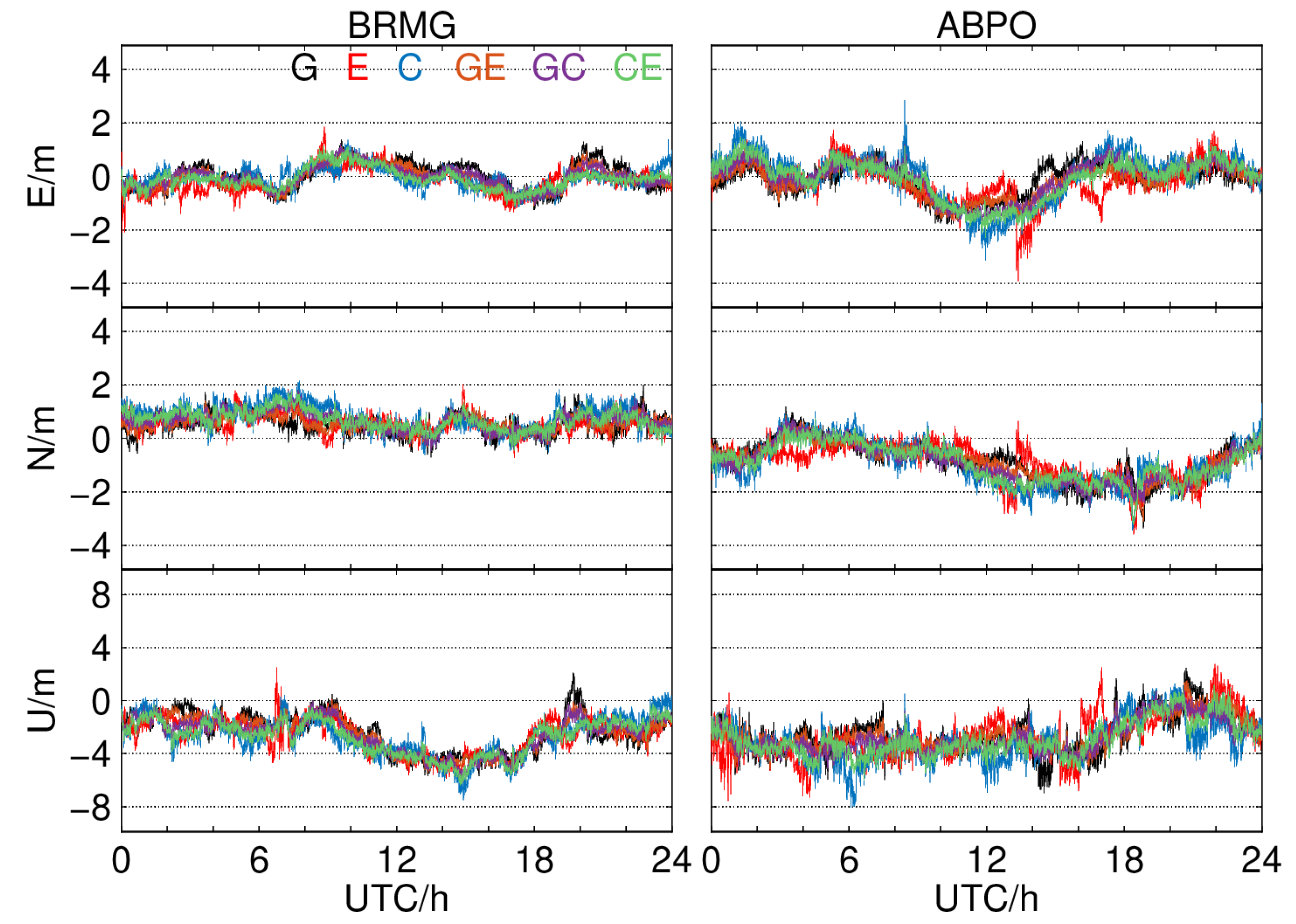
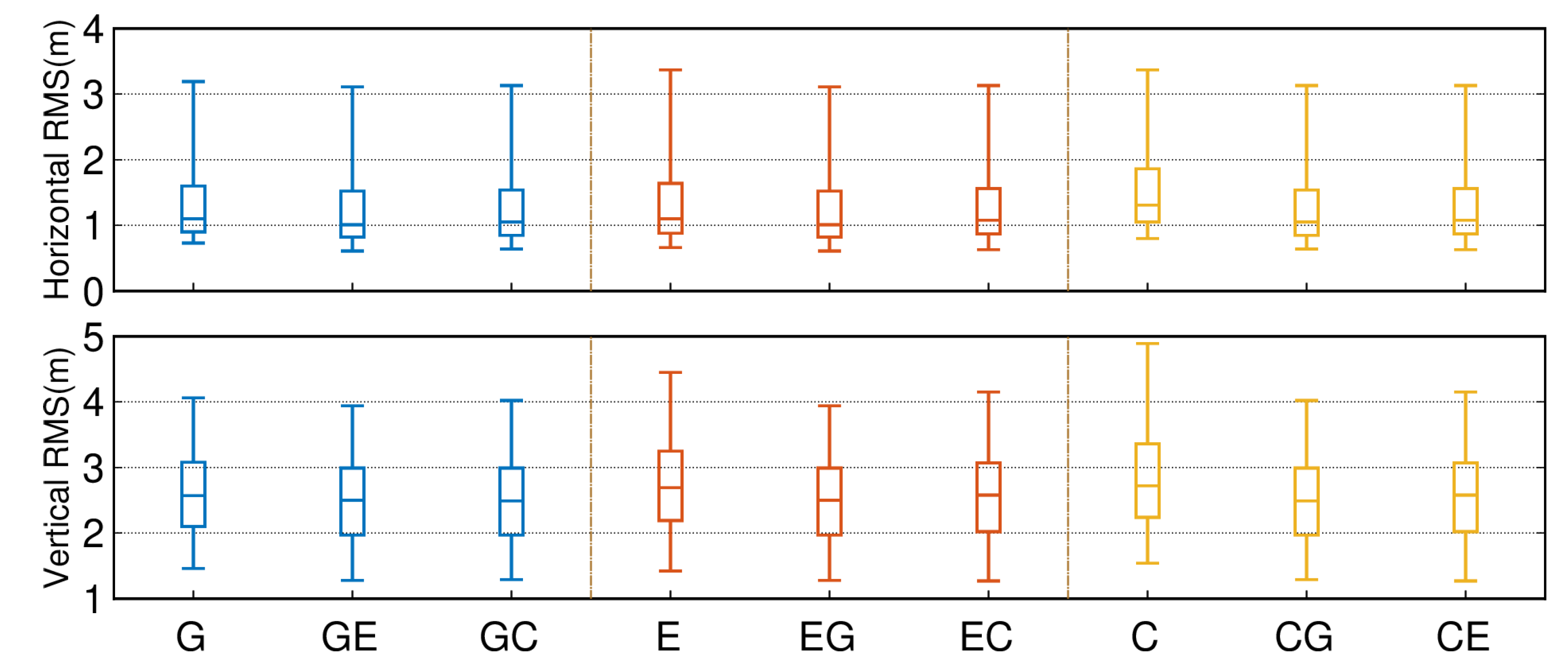
4.4. Dual-System and Single-Frequency SPP (GE, GC, CE)

Due to the few available satellites in a single system, the positioning accuracy of a single-system SPP sometimes cannot match the needs of the users, especially in areas with complex environments. Therefore, to improve the accuracy of the positioning, we added the other systems to the current system separately, using a dual system for SPP. First, we analyzed the positioning errors of the BRMG and ABPO tracking stations GE, GC, and CE for one day. As shown in Figure 13, the error trends of the single and dual systems are similar within one day, and both have system errors. The system error in the E component is not obvious regarding both stations, while the system error in the N component is about 1 m, and the system error in the U component is 2–3 m. In addition, although the trends are similar, the dual system has fewer error fluctuations and fewer coarse differences in one day compared to the single system.

Then, we discussed the overall RMS of the dual system for the 145 tracking stations and the geographic distribution of the gain cases. The boxplot of the positioning accuracy for the dual system combination is displayed in Figure 14.

Table 3. Gain of positioning accuracy of other systems to the current system.

Component	Sys	Negative Gain	Median	Positive Gain	Median
Horizontal	GE	13	−3.2%	132	7.4%
	GC	14	−3.6%	131	14.2%
	EG	2	−2.0%	143	7.2%
	EC	17	−1.2%	128	12.2%
	CG	20	−1.6%	125	5.5%
	CE	51	−3.0%	94	5.4%
Vertical	GE	24	−2.2%	121	6.9%
	GC	20	−2.9%	125	8.4%
	EG	28	−1.0%	117	5.2%
	EC	24	−4.2%	121	7.3%
	CG	28	−1.7%	117	4.6%
	CE	30	−1.9%	115	5.2%

provides the number of tracking stations with the positive and negative gains from other systems for the current system, as well as the median value of the specific gain percentages for the 145 tracking stations. In the horizontal component, the addition of the GPS and Galileo to BDS-3 resulted in accuracy gains for 131 and 128 tracking stations, respectively, with median percentage gains of 14.2% and 12.2%, respectively. The stations with the largest improvements are mainly in Europe and South America. On the contrary, with the addition of BDS-3 to GPS and Galileo, the stations with greater accuracy improvements are mainly in the Asia-Pacific region, and with the addition of Galileo to GPS, only two stations have reduced accuracy, with a percentage improvement of 7.2%. In the vertical component, the GPS provides the largest contribution to BDS-3 with 125 improvements, and the median improvement is 8.3%. The improvements of BDS-3 to GPS and Galileo are mainly concentrated in the Asia-Pacific region and near the equator. In summary, GE has the best positioning accuracy, GC is the second best, and CE is the worst; the GPS has the largest gain on BDS-3, and the number of tracking stations whose accuracy has been improved by adding Galileo to GPS is the largest.

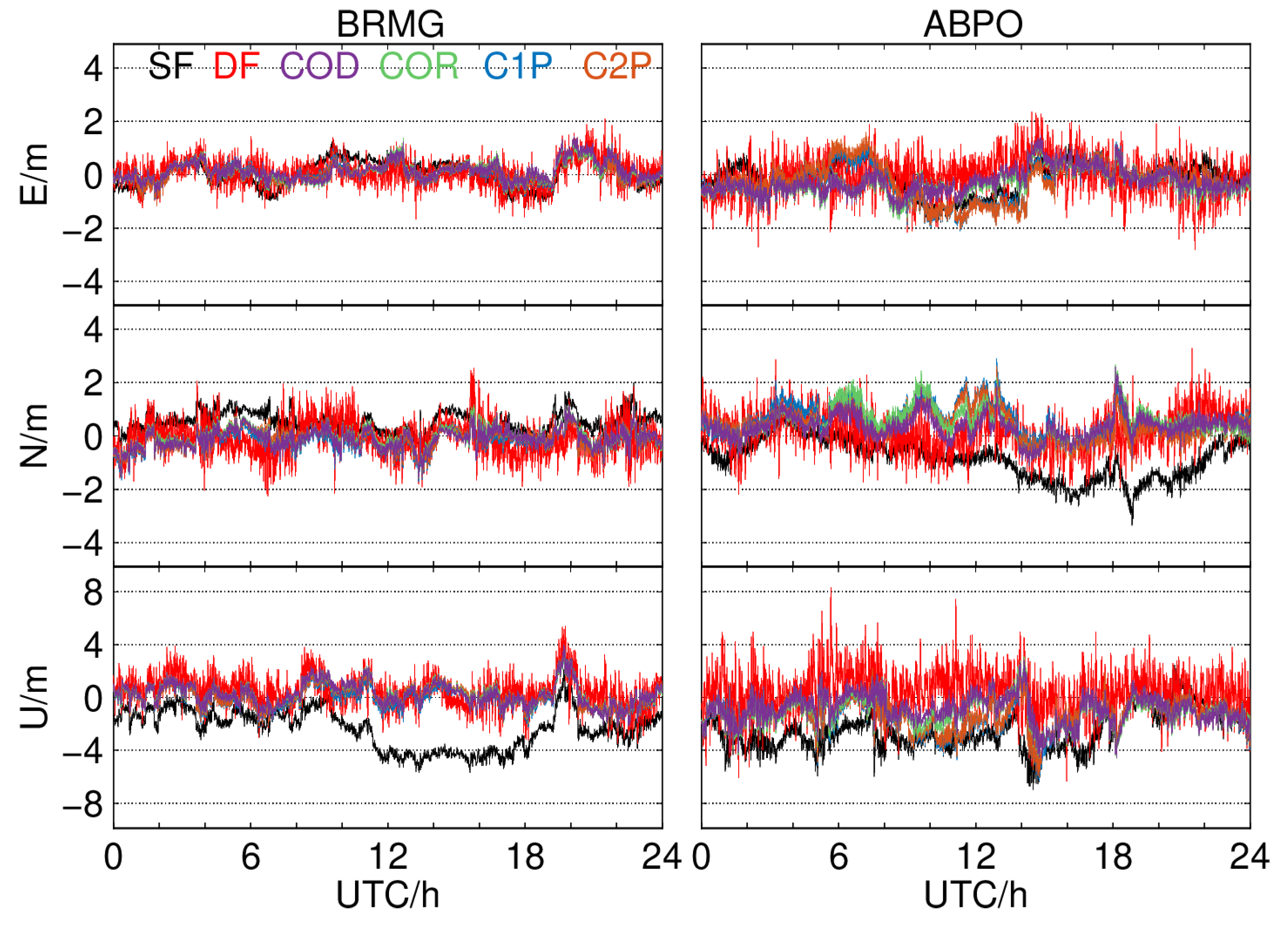
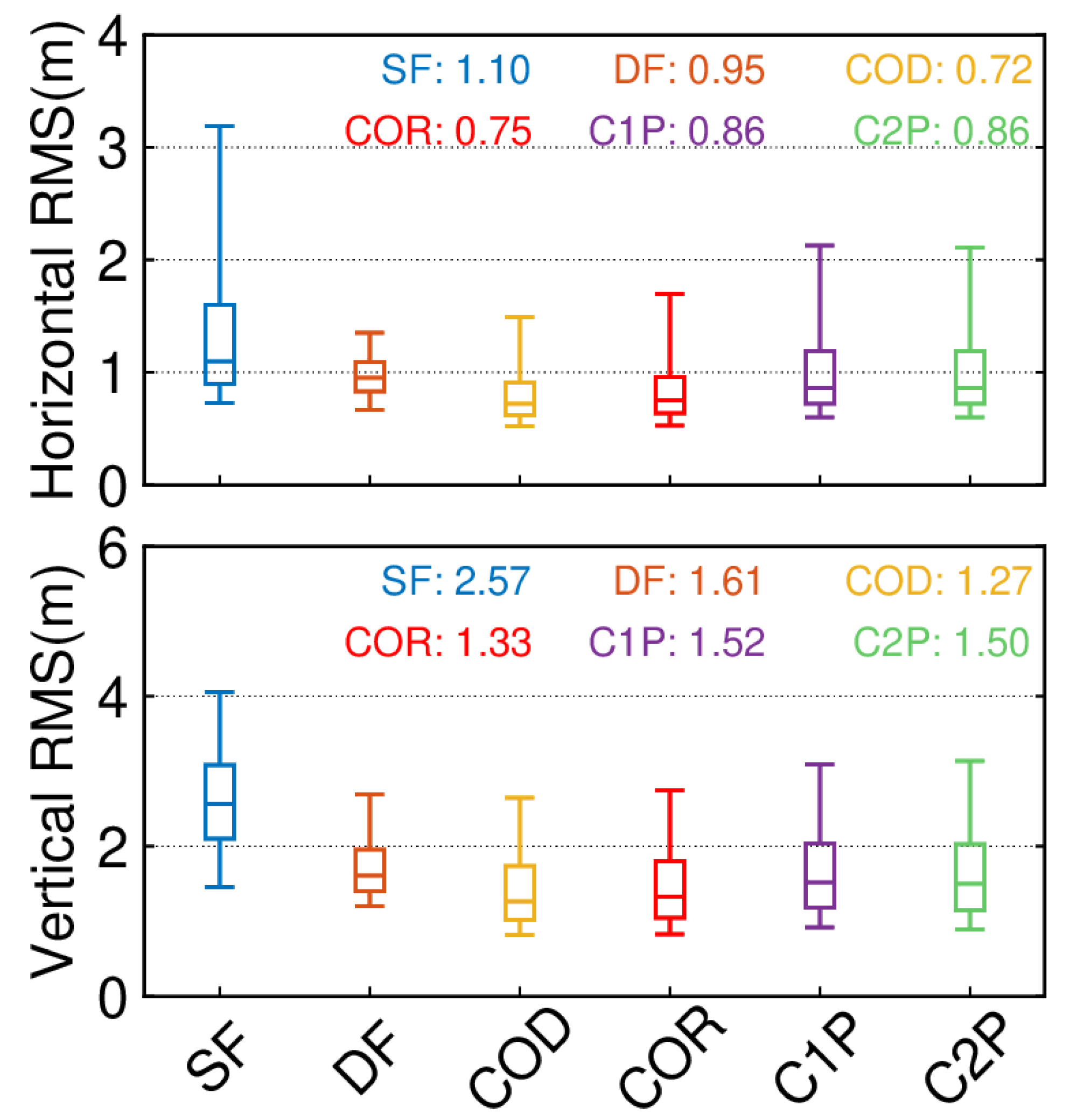
4.5. SPP with GIM Products

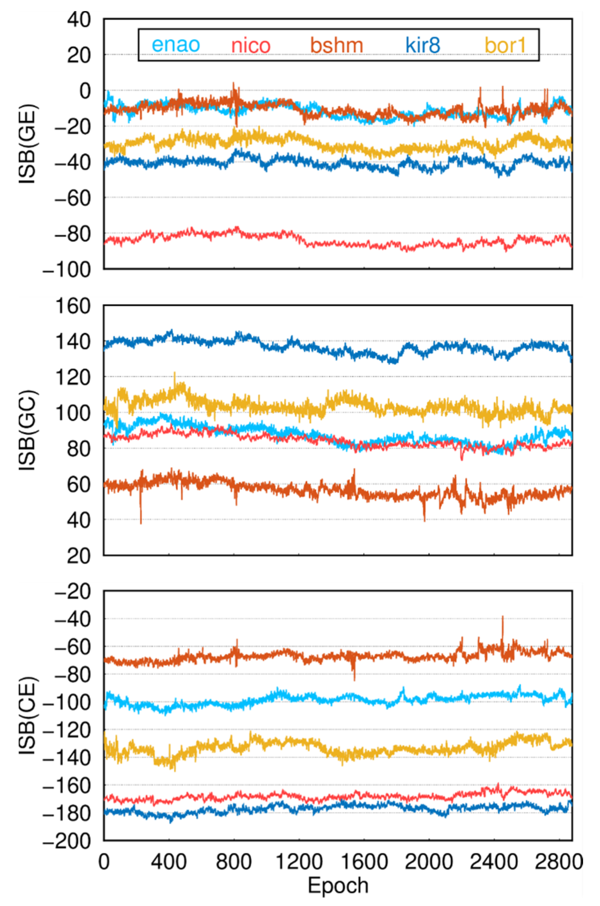
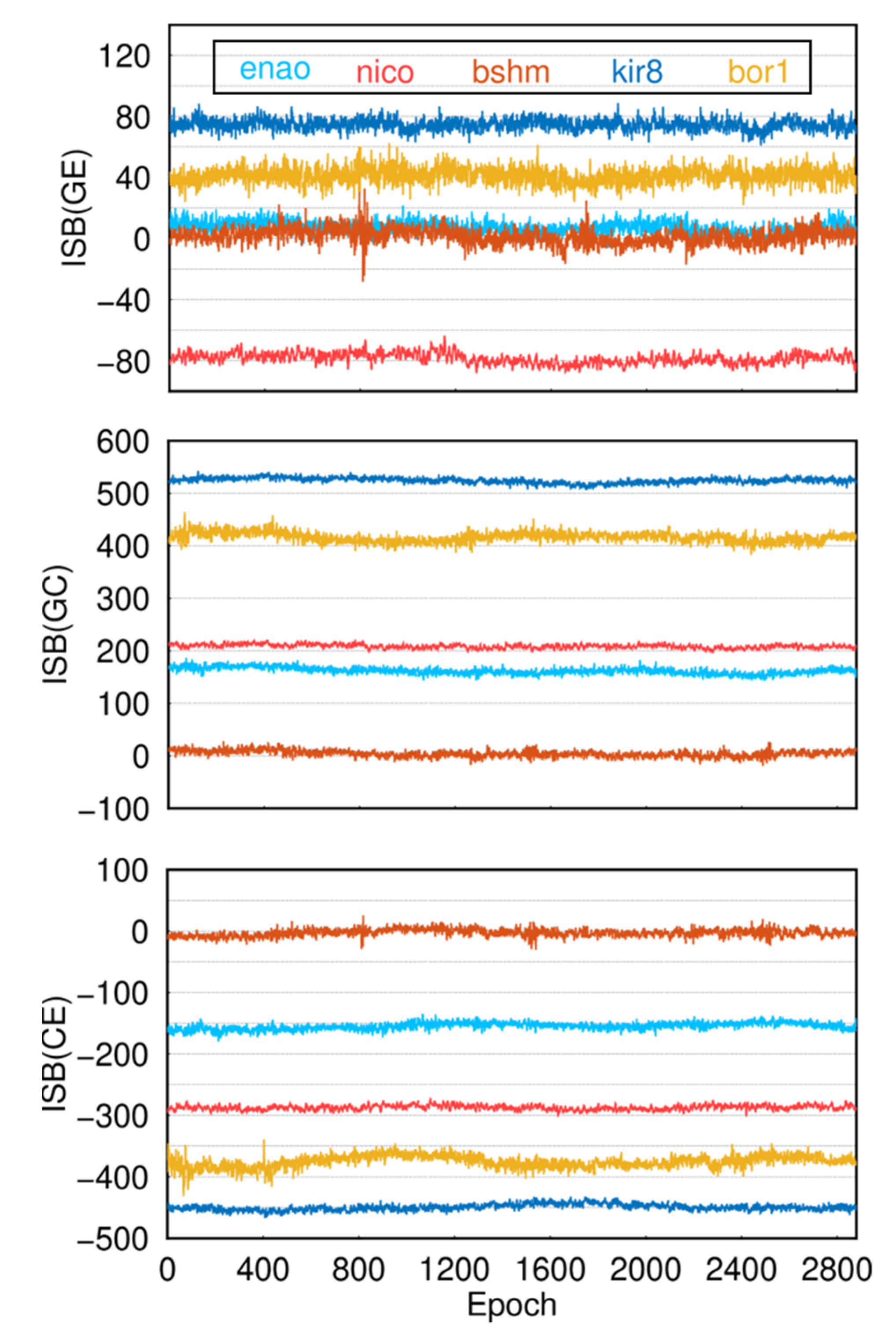
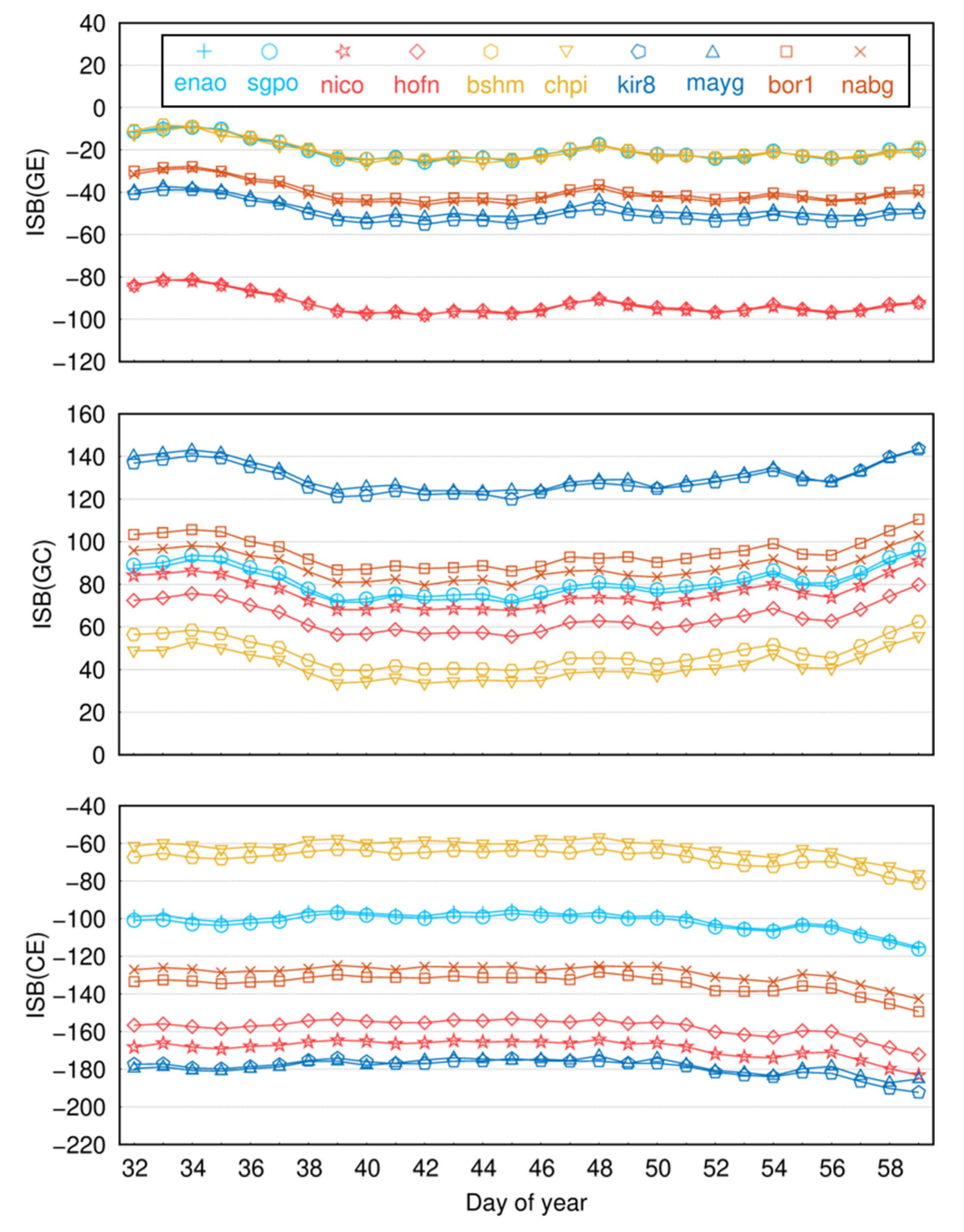
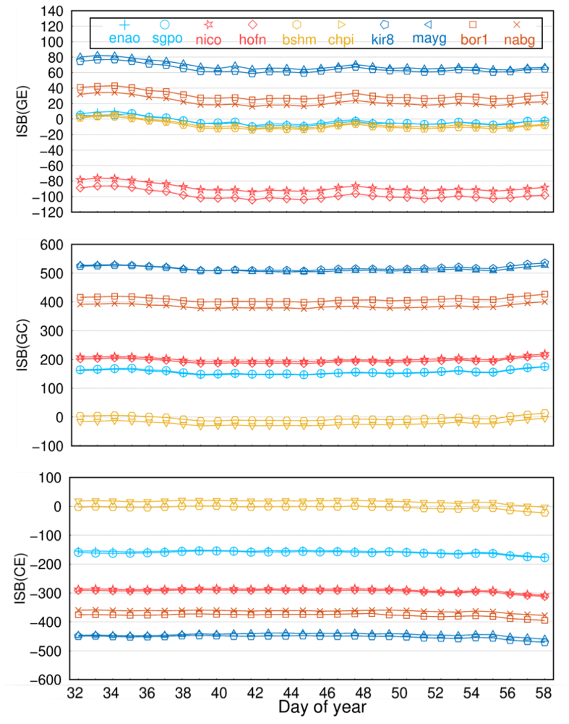
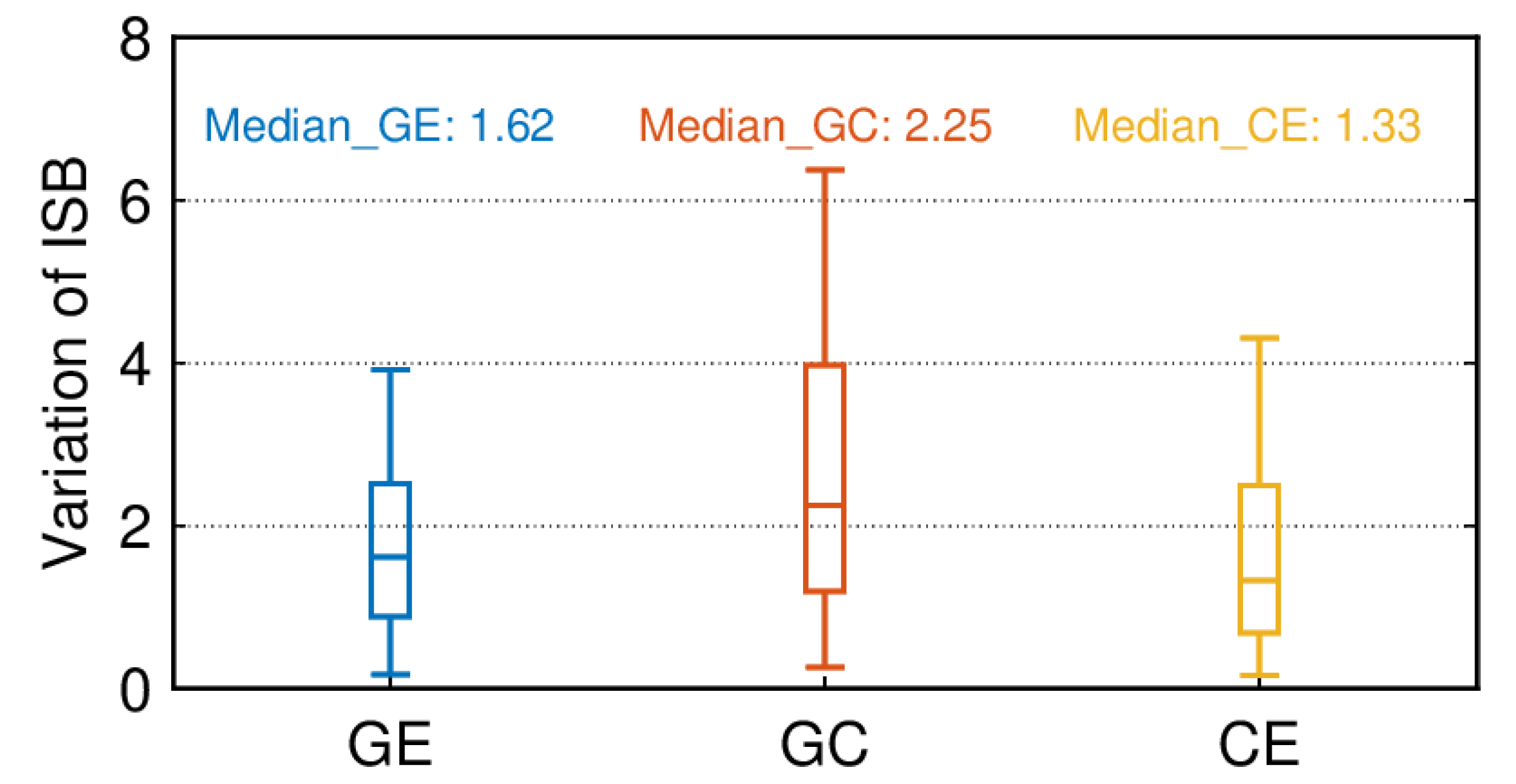
This subsection analyzes the SPP positioning accuracy using different ionospheric products. We used a total of four ionospheric products, COD is the CODE (Center for Orbit Determination in Europe, University of Berne, Switzerland) final global ionospheric map (GIM), COR is the CODE rapid GIM, and C1P and C2P are 1- and 2-day vertical TEC (VTEC) maps produced by CODE (European Centre for Orbitometry, University of Bern, Switzerland), respectively. Figure 15 shows a one-day positioning error sequence for the BRMG and ABPO tracking stations, with large error fluctuations and systematic errors for the single frequency. The error variation trends of COD, COR, C1P, and C2P are similar and have high accuracy.

Figure 16 presents the boxplot of the positioning accuracy for 145 stations using different ionospheric products. In the horizontal component, the median RMSs of SF/DF/COD/COR/C1P/C2P are 1.10/0.95/0.72/0.75/0.86/0.86 m, respectively, and several products have different degrees of median RMS improvements compared with single-frequency and dual-frequency. Additionally, the 95% quantile of C1P and C2P has decreased from more than 3 m to within 2.2 m for a single frequency. COD and COR are even reduced to within 2 m. In the vertical component, the median RMSs of SF/DF/COD/COR/C1P/C2P are 2.57/1.61/1.27/1.33/1.52/1.50 m, respectively. Furthermore, for a single frequency, the 95% quantile of SF, DF, COD, C1P, and C2P is reduced from more than 4 m to less than 3 m. In summary, the highest accuracy is achieved using COD, followed by COR, and C1P and C2 are comparable but slightly worse than COR.

4.6. ISB

The value of ISB can be as high as several thousand nanoseconds, which has a powerful influence on the positioning accuracy of SPP. Therefore, the influence of ISB must be considered in multi-system fusion localization, and this subsection analyzes the stability and variability of ISB. We processed data for a total of 28 days in February 2022 to estimate the ISBs for the GPS with the Galileo combination (GE), the GPS with the BDS-3 combination (GC), and the BDS-3 with the Galileo combination (CE). A total of five receiver types—JAVAD, LEIKA, SEPT, TRIMBLE ALLOY, and TRIMBLE NETR9—were selected for the experimental analysis, and the specific receiver types and numbers are shown in

Table 4. Type and number of receivers.

Receiver	Model	Number
JAVAD	TRE_3	7
	TRE_3 DELTA	17
LEICA	LEICA GR50	8
SEPT	ASTERX4	4
	POLARX5	61
	POLARX5TR	19
TRIMBLE	ALLOY	23
TRIMBLE	NETR9	4

.

First, to analyze the stability of single-frequency and dual-frequency ISBs over a short period, five tracking stations equipped with different receiver types were selected for this paper, and the data selected were for one day on 1 February 2022. As shown in Figure 17 and Figure 18, the single-frequency and dual-frequency ISBs of the five stations vary very little within a day, fluctuating within a certain range, and there is variability in the ISBs of different receivers. To further analyze the variability of ISB, two stations from each of the five receivers were selected to calculate the mean value as well as the standard deviation of the ISB for 28 days in February 2022, and the specific values are displayed in

Table 5. Median and STD of the 28-day single-frequency ISB for the 10 tracking stations (1 February 2022–28 February 2022).

Station	Receiver	G-E		G-C		C-E
		Mean	STD	Mean	STD	Mean	STD
enao	JAVAD TRE_3	−20.51	±4.90	80.24	±6.83	−100.68	±4.68
sgpo	JAVAD TRE_3	−20.49	±4.81	81.43	±6.90	−102.14	±4.51
nico	LEICA GR50	−93.23	±4.89	75.64	±6.66	−169.13	±4.61
yebe	LEICA GR50	−93.44	±4.87	73.9	±6.85	−167.84	±4.76
bshm	SEPT POLARX5	−20.16	±4.89	47.53	±6.69	−67.61	±4.44
chpi	SEPT POLARX5	−20.77	±4.64	41.93	±6.42	−62.12	±4.53
kir8	TRIMBLE ALLOY	−50.15	±4.91	129.33	±6.66	−179.35	±4.62
mayg	TRIMBLE ALLOY	−47.44	±4.41	131.27	±6.46	−178.75	±4.14
bor1	TRIMBLE NETR9	−39.5	±4.96	95.19	±6.75	−134.78	±4.76
nabg	TRIMBLE NETR9	−40.69	±5.02	88.29	±6.39	−128.8	±4.28

and

Table 6. Median and STD of the 28-day dual-frequency ISB for the 10 tracking stations (1 February 2022–28 February 2022).

Station	Receiver	G-E		G-C		C-E
		Mean	STD	Mean	STD	Mean	STD
enao	JAVAD TRE_3	−2.58	±4.13	155.14	±5.78	−157.67	±5.76
sgpo	JAVAD TRE_3	−3.61	±3.95	157.55	±5.50	−161.17	±5.34
nico	LEICA GR50	−88.49	±3.49	201.12	±4.03	−289.62	±4.32
yebe	LEICA GR50	−98.42	±4.03	195.31	±5.09	−293.75	±5.10
bshm	SEPT POLARX5	−8.41	±5.01	−4.26	±6.60	−4.16	±6.64
chpi	SEPT POLARX5	−6.61	±4.02	−22.36	±5.50	−15.86	±5.67
kir8	TRIMBLE ALLOY	−64.94	±4.11	517.59	±5.10	−452.53	±5.01
mayg	TRIMBLE ALLOY	−69.06	±5.16	514.02	±6.33	−444.76	±6.49
bor1	TRIMBLE NETR9	−30.79	±5.57	408.88	±9.74	−377.68	±12.74
nabg	TRIMBLE NETR9	−22.25	±3.82	385.06	±8.44	−386.85	±8.21

.

Figure 19 and Figure 20 show the average ISB values of the single frequency and dual frequency for 10 tracking stations equipped with five receiver types every day of the month. The single-frequency and dual-frequency ISB values of the same receiver type are very close, which may mean that the ISB value is closely related to the hardware delay. The single-frequency ISBs of two tracking stations of the same receiver of GE, GC, and CE are less than 3 ns, 7 ns, and 6 ns, respectively. The dual-frequency ISBs of two tracking stations of the same receiver of GE, GC, and CE are less than 10 ns, 23 ns, and 11 ns, respectively. The ISB value of the dual-frequency SPP is larger, and the ISB of the KIR8 tracking station GC reaches 517.59 ns. Additionally, the ISB difference in stations with the same receiver is also larger than that of the single-frequency ISB, and the ISB difference between the BOR1 and NABG tracking station GC reaches 23 ns; thus, we recommend using single-frequency receivers. In parallel, we used GIM products to estimate the ISB. The difference between the estimated result and the ISB value estimated by a single frequency is very small and can be controlled within 10 ns. In order to verify the stability of the ISBs in the long term, the difference in ISBs for every two adjacent days in a 28-day period is calculated for all tracking stations. The boxplot demonstrating the difference in the ISBs of GE, GC, and CE for two adjacent days is shown in Figure 21, and the difference in the ISBs of GE, GC, and CE for two adjacent days are within 4 ns, 7 ns, and 5 ns (95th percentile), respectively.

5. Conclusions

GNSS was an emerging field in the 20th century, among which SPP has the features of low cost, a fast solution speed, and small hardware size, which can be installed on small devices, such as cell phones and receivers, and has been widely used in car navigation, cell phone terminal positioning, earthquake mitigation and detection, agriculture and forestry, and other fields. In this paper, 145 tracking stations were selected to analyze the positioning theory of SPP and its positioning performance, and the following conclusions were obtained:

(1) First, we analyzed the satellite availability and PDOP values of the GPS, Galileo, BDS-3-MEO, BDS-3-MEO+IGSO, and BDS-3-MEO+IGSO+GEO. The results indicate that the global satellite availabilities of the GPS, Galileo, and BDS-3-MEO have similar global distributions, all of which first decrease and then increase from the equator to the poles. In the mid and low latitudes, the number of available satellites is 11/8/9, respectively. In other regions, the number of available satellites increases to 13, 10, and 10, respectively. However, when the IGSO and GEO satellites are added, the number of available satellites increases to 12 for BDS-3 and reaches 13 near the equator in the Eastern hemisphere. The number of available satellites in the Eastern hemisphere is strongly enhanced.

(2) The accuracy of the global distribution of the GPS, BDS-3, and Galileo single-frequency SPP is analyzed, while the accuracy distribution characteristics of the three systems are compared globally. The results show that in the horizontal component, the GPS and Galileo have the best positioning accuracy of 1–1.2 m in Europe and North America and 2–3 m at low latitudes, while BDS-3 has the highest positioning accuracy of about 1.2 m in the Asia-Pacific region, and the overall Eastern hemisphere is better than the Western hemisphere. In the vertical component, the accuracy of all three systems gradually deteriorates from south to north, probably due to system bias and perhaps due to the influence of the ionosphere. After the comparison of the three systems, the positioning accuracy of the GPS and Galileo is comparable, and BDS-3 outperforms the GPS and Galileo by 30% and 20% in the Asia-Pacific region on the horizontal and vertical components, respectively.

(3) We combined BDS-3 or Galileo with GPS, GPS or Galileo with BDS-3, and GPS or BDS-3 with Galileo and analyzed the percentage gain of the combined SPP with respect to the single system. The conclusions drawn are as follows: For the combination of the GPS and Galileo with BDS-3, the accuracy of the Asia-Pacific region in the horizontal and vertical components will be improved by 30% and 20%, respectively. When the GPS and Galileo are combined with BDS-3, the accuracy in North America and Europe will improve by 30–40% in the horizontal component, and the global accuracy will improve by 10–20% in the vertical component. The combination of Galileo and the GPS or BDS-3 can effectively improve the accuracy of the vertical component in the middle and low latitudes by about 15–20%.

(4) We analyzed the positioning accuracy using different ionospheric products, and the results showed that the median RMS of COD, COR, C1P, and C2P were 0.72/0.75/0.86/0.86 m and 1.27/1.33/1.52/1.50 m, respectively, with the highest accuracy using COD, followed by COR, and C1P and C2P being comparable and slightly lower than COR, thus providing a reference to facilitate the selection of products for single-frequency GNSS users.

(5) We analyzed the positioning accuracy using different ionospheric products, and the results showed that the single-frequency positioning accuracy was the worst, with the highest accuracy using COD, followed by COR, and C1P and C2P being equivalent and slightly lower than COR.

(6) Finally, we analyzed the single-frequency and dual-frequency ISBs of five receiver types, and the results showed that the ISBs are stable in a short time. At the same time, the ISB is related to the receiver type, and the difference between the single-frequency ISB of the same receiver type is smaller than that of the dual-frequency ISB; thus, it is recommended to use the single-frequency receiver.

The results of this paper clearly illustrate the positioning accuracy of three single-system SPP solutions—GPS, BDS-3, and Galileo—in different regions. As well as being able to analyze the positioning superiority of different system combinations in different regions, this provides a reference for choosing the optimal combination for different regions, while the ISB analysis provides more possibilities for the multi-system combination SPP.

References

1. Zheng, F.; Gu, S.; Gong, X.; Lou, Y.; Fan, L.; Shi, C. Real-time single-frequency pseudorange positioning in China based on regional satellite clock and ionospheric models. GPS Solut. 2020, 24, 6. [Google Scholar] [CrossRef]
2. Hu, J.; Li, P.; Zhang, X.; Bisnath, S.; Pan, L. Precise point positioning with BDS-2 and BDS-3 constellations: Ambiguity resolution and positioning comparison. Adv. Space Res. 2022, 70, 1830–1846. [Google Scholar] [CrossRef]
3. Zhou, F.; Li, X.; Li, W.; Chen, W.; Dong, D.; Wickert, J.; Schuh, H. The Impact of Estimating High-Resolution Tropospheric Gradients on Multi-GNSS Precise Positioning. Sensors 2017, 17, 756. [Google Scholar] [CrossRef]
4. Ma, H.; Psychas, D.; Xing, X.; Zhao, Q.; Verhagen, S.; Liu, X. Influence of the inhomogeneous troposphere on GNSS positioning and integer ambiguity resolution. Adv. Space Res. 2021, 67, 1914–1928. [Google Scholar] [CrossRef]
5. Paziewski, J.; Wielgosz, P. Assessment of GPS + Galileo and multi-frequency Galileo single-epoch precise positioning with network corrections. GPS Solut. 2014, 18, 571–579. [Google Scholar] [CrossRef] [Green Version]
6. Liu, J.; Cao, C. Development status and trend of global navigation satellite system. J. Navig. Position. 2020, 8, 1–8. [Google Scholar] [CrossRef]
7. Yang, Z.; Xue, B. The developed procedures and developing trends of the American navigation satellites. J. Navig. Position. 2021, 9, 1–12. [Google Scholar] [CrossRef]
8. Montenbruck, O.; Steigenberger, P.; Hauschild, A. Broadcast versus precise ephemerides: A multi-GNSS perspective. GPS Solut. 2015, 19, 321–333. [Google Scholar] [CrossRef]
9. Xu, Y.; Ji, S. Data quality assessment and the positioning performance analysis of BeiDou in Hong Kong. Surv. Rev. 2015, 47, 446–457. [Google Scholar] [CrossRef]
10. Robustelli, U.; Pugliano, G. Galileo Single Point Positioning Assessment Including FOC Satellites in Eccentric Orbits. Remote Sens. 2019, 11, 1555. [Google Scholar] [CrossRef]
11. CSNO. The Current Constellation of the BDS System. China Satellite Navigation Office. 2021. Available online: http://www.csno-tarc.cn/system/constellation (accessed on 2 June 2022).
12. Yang, Z.; Xue, B. The developed procedures and developing trends of BeiDou satellite navigation system. J. Navig. Position. 2022, 10, 1–14. [Google Scholar] [CrossRef]
13. Yang, Y.; Li, J.; Wang, A.; Xu, J.; He, H.; Guo, H.; Shen, J.; Dai, X. Preliminary assessment of the navigation and positioning performance of BeiDou regional navigation satellite system. Sci. China Earth Sci. 2014, 57, 144–152. [Google Scholar] [CrossRef]
14. Guo, F.; Zhang, X.; Wang, J. Timing group delay and differential code bias corrections for BeiDou positioning. J. Geod. 2015, 89, 427–445. [Google Scholar] [CrossRef]
15. Padokhin, A.M.; Mylnikova, A.A.; Yasyukevich, Y.V.; Morozov, Y.V.; Kurbatov, G.A.; Vesnin, A.M. Galileo E5 AltBOC Signals: Application for Single-Frequency Total Electron Content Estimations. Remote. Sens. 2021, 13, 3973. [Google Scholar] [CrossRef]
16. Luo, X.; Lou, Y.; Gong, X.; Gu, S.; Chen, B. Benefit of Sparse Reference Network in BDS Single Point Positioning with Single-Frequency Measurements. J. Navig. 2018, 71, 403–418. [Google Scholar] [CrossRef]
17. Zhang, Z.; Pan, L. Current performance of open position service with almost fully deployed multi-GNSS constellations: GPS, GLONASS, Galileo, BDS-2, and BDS-3. Adv. Space Res. 2022, 69, 1994–2019. [Google Scholar] [CrossRef]
18. Blanco-Delgado, N.; Nunes, F.D. Satellite selection based on WDOP concept and convex geometry. In Proceedings of the 2010 5th ESA Workshop on Satellite Navigation Technologies and European Workshop on GNSS Signals and Signal Processing (NAVITEC), Noordwijk, The Netherlands, 8–10 December 2010; pp. 1–8. [Google Scholar] [CrossRef]
19. Klobuchar, J.A. Ionospheric Time-Delay Algorithm for Single-Frequency GPS Users. IEEE Trans. Aerosp. Electron. Syst. 1987, 3, 325–331. [Google Scholar] [CrossRef]
20. Wu, X.; Hu, X.; Wang, G.; Zhong, H.; Tang, C. Evaluation of COMPASS ionospheric model in GNSS positioning. Adv. Space Res. 2013, 51, 959–968. [Google Scholar] [CrossRef]
21. Yang, C.; Guo, J.; Geng, T.; Zhao, Q.; Jiang, K.; Xie, X.; Lv, Y. Assessment and Comparison of Broadcast Ionospheric Models: NTCM-BC, BDGIM, and Klobuchar. Remote Sens. 2020, 12, 1215. [Google Scholar] [CrossRef]
22. Li, Q.; Su, X.; Xu, Y.; Ma, H.; Liu, Z.; Cui, J.; Geng, T. Performance Analysis of GPS/BDS Broadcast Ionospheric Models in Standard Point Positioning during 2021 Strong Geomagnetic Storms. Remote Sens. 2022, 14, 4424. [Google Scholar] [CrossRef]
23. Li, M.; Yuan, Y.; Wang, N.; Li, Z.; Huo, X. Performance of various predicted GNSS global ionospheric maps relative to GPS and JASON TEC data. GPS Solut. 2018, 22, 55. [Google Scholar] [CrossRef]
24. Pan, L.; Cai, C.; Santerre, R.; Zhang, X. Performance evaluation of single-frequency point positioning with GPS, GLONASS, BeiDou and Galileo. Surv. Rev. 2017, 49, 197–205. [Google Scholar] [CrossRef]
25. Ryan, S.; Petovello, M.; Lachapelle, G. Augmentation of GPS for Ship Navigation in Constricted Water Ways. In Proceedings of the 1998 National Technical Meeting of The Institute of Navigation, Long Beach, CA, USA, 21–23 January 1998; pp. 459–467. [Google Scholar]
26. Cai, C.; Gao, Y.; Pan, L.; Dai, W. An analysis on combined GPS/COMPASS data quality and its effect on single point positioning accuracy under different observing conditions. Adv. Space Res. 2014, 54, 818–829. [Google Scholar] [CrossRef]
27. Cai, C.; Luo, X.; Liu, Z.; Xiao, Q. Galileo Signal and Positioning Performance Analysis Based on Four IOV Satellites. J. Navig. 2014, 67, 810–824. [Google Scholar] [CrossRef] [Green Version]
28. Odolinski, R.; Teunissen, P.J.G.; Odijk, D. First combined COMPASS/BeiDou-2 and GPS positioning results in Australia. Part I: Single-receiver and relative code-only positioning. J. Spat. Sci. 2014, 59, 3–24. [Google Scholar] [CrossRef]
29. Yang, Y.; Xu, J. GNSS receiver autonomous integrity monitoring (RAIM) algorithm based on robust estimation. Geod. Geodyn. 2016, 7, 117–123. [Google Scholar] [CrossRef] [Green Version]
30. Wang, J.; Knight, N.L.; Lu, X. Impact of the GNSS Time Offsets on Positioning Reliability. J. Glob. Position. Syst. 2011, 10, 165–172. [Google Scholar] [CrossRef] [Green Version]
31. Teng, Y.; Wang, J. New Characteristics of Geometric Dilution of Precision (GDOP) for Multi-GNSS Constellations. J. Navig. 2014, 67, 1018–1028. [Google Scholar] [CrossRef]
32. Montenbruck, O.; Hauschild, A.; Hessels, U. Characterization of GPS/GIOVE sensor stations in the CONGO network. GPS Solut. 2011, 15, 193–205. [Google Scholar] [CrossRef]
33. Zeng, A.; Yang, Y.; Ming, F.; Jing, Y. BDS–GPS inter-system bias of code observation and its preliminary analysis. GPS Solut. 2017, 21, 1573–1581. [Google Scholar] [CrossRef]
34. Zhou, F.; Dong, D.; Li, W.; Jiang, X.; Wickert, J.; Schuh, H. GAMP: An open-source software of multi-GNSS precise point positioning using undifferenced and uncombined observations. GPS Solut. 2018, 22, 33. [Google Scholar] [CrossRef]
35. Yang, Y.; Li, J.; Xu, J.; Tang, J.; Guo, H.; He, H. Contribution of the Compass satellite navigation system to global PNT users. Chin. Sci. Bull. 2011, 56, 2813–2819. [Google Scholar] [CrossRef] [Green Version]
36. Geng, J.; Meng, X.; Dodson, A.H.; Teferle, F.N. Integer ambiguity resolution in precise point positioning: Method comparison. J. Geod. 2010, 84, 569–581. [Google Scholar] [CrossRef]
Figure 1. Geographical distribution of 145 tracking stations.
Remotesensing 15 00797 g001
Figure 2. Number of visible satellites for GPS, Galileo, BDS-3-MEO, BDS-3-MEO+IGSO, and BDS-3-MEO+IGSO+GEO.
Remotesensing 15 00797 g002
Figure 3. The PDOP for GPS, Galileo, BDS-3-MEO, BDS-3-MEO+IGSO, and BDS-3-MEO+IGSO+GEO.
Remotesensing 15 00797 g003
Figure 4. Geographical distribution of positioning accuracy of 145 tracking stations in 3D with IGSO and GEO satellites added to MEO.
Remotesensing 15 00797 g004
Figure 5. Single-frequency positioning errors for the E, N, and U components of the two tracking stations of BRMG and ABPO.
Remotesensing 15 00797 g005
Figure 6. Number of visible satellites and PDOP values for the two tracking stations, BRMG and ABPO.
Remotesensing 15 00797 g006
Figure 7. Boxplot of position accuracy of single-frequency SPP with an elevation cut-off of 7° for GPS, Galileo, and BDS-3.
Remotesensing 15 00797 g007
Figure 8. Geographical distribution of positioning accuracy of 145 tracking stations in horizontal and vertical components with an elevation cut-off of 7° for GPS, Galileo, and BDS-3.
Remotesensing 15 00797 g008
Figure 9. Geographical distribution of the single-frequency positioning accuracy of 145 tracking stations in the horizontal and vertical sections of GPS, Galileo and BDS-3.
Remotesensing 15 00797 g009
Figure 10. Dual-frequency positioning errors for the E, N, and U components of the two tracking stations of BRMG and ABPO.
Remotesensing 15 00797 g010
Figure 11. Boxplot of position accuracy of dual-frequency ionosphere-free combined SPP with an elevation cut-off of 7° for GPS, Galileo, and BDS-3.
Remotesensing 15 00797 g011
Figure 12. Geographical distribution of the dual-frequency positioning accuracy of 145 tracking stations in the horizontal and vertical sections of GPS, Galileo and BDS-3.
Remotesensing 15 00797 g012
Figure 13. Dual system positioning errors for the E, N, and U components of the two tracking stations of BRMG and ABPO.
Remotesensing 15 00797 g013
Figure 14. Boxplot of position accuracy of dual system with an elevation cut-off of 7°.
Remotesensing 15 00797 g014
Figure 15. SPP positioning accuracy of different ionospheric products for BRMG and ABPO tracking stations.
Remotesensing 15 00797 g015
Figure 16. Boxplot of positioning accuracy of 145 tracking stations for different ionospheric products.
Remotesensing 15 00797 g016
Figure 17. One-day single-frequency ISB of 5 tracking stations equipped with different receivers (1 February 2022).
Remotesensing 15 00797 g017
Figure 18. One-day dual-frequency ISB of 5 tracking stations equipped with different receivers (1 February 2022).
Remotesensing 15 00797 g018
Figure 19. Average value of daily single-frequency ISB for 10 tracking stations of 5 receivers.
Remotesensing 15 00797 g019
Figure 20. Average value of daily dual-frequency ISB for 10 tracking stations of 5 receivers.
Remotesensing 15 00797 g020
Figure 21. Boxplot of variation of ISB for two days adjacent to all tracking stations (1 February 2022 to 28 February 2022).
Remotesensing 15 00797 g021