Article

Comparisons of Convolutional Neural Network and Other Machine Learning Methods in Landslide Susceptibility Assessment: A Case Study in Pingwu

1
School of National Safety and Emergency Management, Beijing Normal University, 19 Xinjiekou Wai Ave., Beijing 100875, China
2
Faculty of Geographical Science, Beijing Normal University, 19 Xinjiekou Wai Ave., Beijing 100875, China
*
Author to whom correspondence should be addressed.
Remote Sens. 2023, 15(3), 798; https://doi.org/10.3390/rs15030798
Submission received: 14 December 2022 / Revised: 18 January 2023 / Accepted: 24 January 2023 / Published: 31 January 2023

Abstract

:
Landslide is a natural disaster that seriously affects human life and social development. In this study, the characteristics and effectiveness of convolutional neural network (CNN) and conventional machine learning (ML) methods in a landslide susceptibility assessment (LSA) are compared. Six ML methods used in this study are Adaboost, multilayer perceptron neural network (MLP-NN), random forest (RF), naive Bayes, decision tree (DT), and gradient boosting decision tree (GBDT). First, the basic knowledge and structures of the CNN and ML methods, and the steps of the LSA are introduced. Then, 11 conditioning factors in three categories in the Hongxi River Basin, Pingwu County, Mianyang City, Sichuan Province are chosen to build the train, validation, and test samples. The CNN and ML models are constructed based on these samples. For comparison, indicator methods, statistical methods, and landslide susceptibility maps (LSMs) are used. The result shows that the CNN can obtain the highest accuracy (86.41%) and the highest AUC (0.9249) in the LSA. The statistical methods represented by the mean and variance of TP and TN perform more firmly on the possibility of landslide occurrence. Furthermore, the LSMs show that all models can successfully identify most of the landslide points, but for areas with a low frequency of landslides, some models are insufficient. The CNN model demonstrates better results in the recognition of the landslides’ cluster region, this is also related to the convolution operation that takes the surrounding environment information into account. The higher accuracy and more concentrative possibility of CNN in LSA is of great significance for disaster prevention and mitigation, which can help the efficient use of human and material resources. Although CNN performs better than other methods, there are still some limitations, the identification of low-cluster landside areas can be enhanced by improving the CNN model.

1. Introduction

Landslide is one of the most common natural disasters worldwide. Landslide refers to the natural phenomenon in which the soil or rock mass on the slope slides down [1]. They are usually triggered by heavy rainfall [2,3] or earthquakes [4]. When landslides occur, it has an important impact on the safety of people [5], social and economic development [6], and regional design and planning [7]. In recent years, landslides have gradually attracted the attention of the government and many scholars due to their great harm to society. A large number of studies have been carried out on the occurrence mechanism [8], risk analysis [9], and susceptibility assessment [10] of landslides. The disaster-causing process and efficient disaster prevention and mitigation work are of great significance [11,12].
Landslide susceptibility assessment (LSA) refers to the use of some methods to assess the spatial distribution of the possibility of landslide occurrence in an area, based on historical landslide events and related conditioning factors. Traditional research on landslide susceptibility mainly includes the expert experience method and statistical analysis methods [13,14]. Experts can make judgments about the susceptibility of landslides, based on their experience working with landslides and in conjunction with the physical mechanisms of landslides. Statistical analysis refers to the use of correlation analysis [14], frequency analysis [15], analytic hierarchy [13], and other methods to find the relationship between landslide conditioning factors and landslides [16]. According to the contribution rate of these conditioning factors and landslide points, the landslide susceptibility of an area can be assessed.
In recent years, the rapid development of computer technology and the continuous innovation of hardware and software have greatly promoted the development of deep learning (DL) and machine learning (ML). Because of its powerful data processing, feature extraction, and autonomous learning capabilities [17,18,19], DL is not only regarded as the core to promote the future development of artificial intelligence (AI) but has also been introduced into many disciplines, such as medicine [20], astronomy [21], and geography [22]. ML and DL simulate human thinking, based on mathematical statistics methods to gain more knowledge and finally achieve many functions, based on this knowledge. Based on ML, DL [23] provides a more in-depth study of the relevant information within the data, such as convolutional neural network (CNN) [17], long short-term memory neural network (LSTM) [24], and deep neural network (DNN) [25]. In the case of big data samples, the DL can gain more in-depth and rich knowledge than ML. In the field of natural disasters [22,26,27], ML and DL have been used, and good results have been obtained in disaster detection [28], susceptibility analysis [22], disaster forecasting [29], and so on.
There are many studies in LSA using ML or DL methods. Related studies can be mainly divided into three categories, the comparison of several ML methods, comparison of ML and DL methods, and using improved ML or DL methods in LSA. Previous studies have focused more on the performance of the model. In this study, focus is on the differences between CNN and ML results, as well as the reasons for such differences, by comparing the spatial distribution of landslide susceptibility and some statistical features derived from CNN and ML methods. The DL method used is CNN [17]. CNN is a classic DL method, it is also relatively mature, and can represent the idea of DL to a certain extent. Conventional ML methods used for comparison are Adaboost, multilayer perceptron neural network (MLP-NN), random forest (RF), naive Bayes, decision tree (DT), and gradient boosting decision tree (GBDT). These six ML methods have been used extensively and have demonstrated that they can obtain good results when dealing with geographic problems [30,31,32]. The principle of CNN and ML in LSA is to learn more about the relationship of the conditioning factors and landslide points. However, the CNN also takes the information of the conditioning factors around the landslide points into consideration, which is more consistent with the geographical characteristics. Hongxi River Basin in Pingwu County, Mianyang City, Sichuan Province, China, is chosen as a case study for this comparison.

2. Materials and Methods

2.1. Study Area

The case study area is located in the Hongxi River Basin, Pingwu County, Mianyang City, Sichuan Province, China (Figure 1). The climate is mild and the rainfall is sufficient. This area is dominated by mountains, with elevations between 674 m and 2256 m. It is located in the seismic zone of the Qinghai-Tibet Plateau, and earthquakes occur frequently, which has also led to a high frequency of landslides over the past several years. This area is also prone to rainfall, and the materials produced by landslides accumulate in rivers or valleys. This also leads to the formation of landslides again by the loose materials and landslide-prone points after subsequent earthquakes or rainfall [33]. The occurrence of long-term landslides has seriously affected the development of the local economy and threatened the lives of residents.

2.2. Data

The data used in this study include landslide points data and 11 landslide conditioning factors. Following the 2008 Wenchuan earthquake, many landslides occurred in the study area. The landslide areas in this study are obtained through visual interpretation of remote sensing images, and landslide points are generated from the landslide area. In this way, 962 landslide points are used. For comparison, the same number of non-landslide points are randomly generated in the study area outside the landslide area through ArcGIS. These landslides are earthquake-induced landslides and not rainfall-induced landslides, despite the relatively frequent rainfall in this study area.
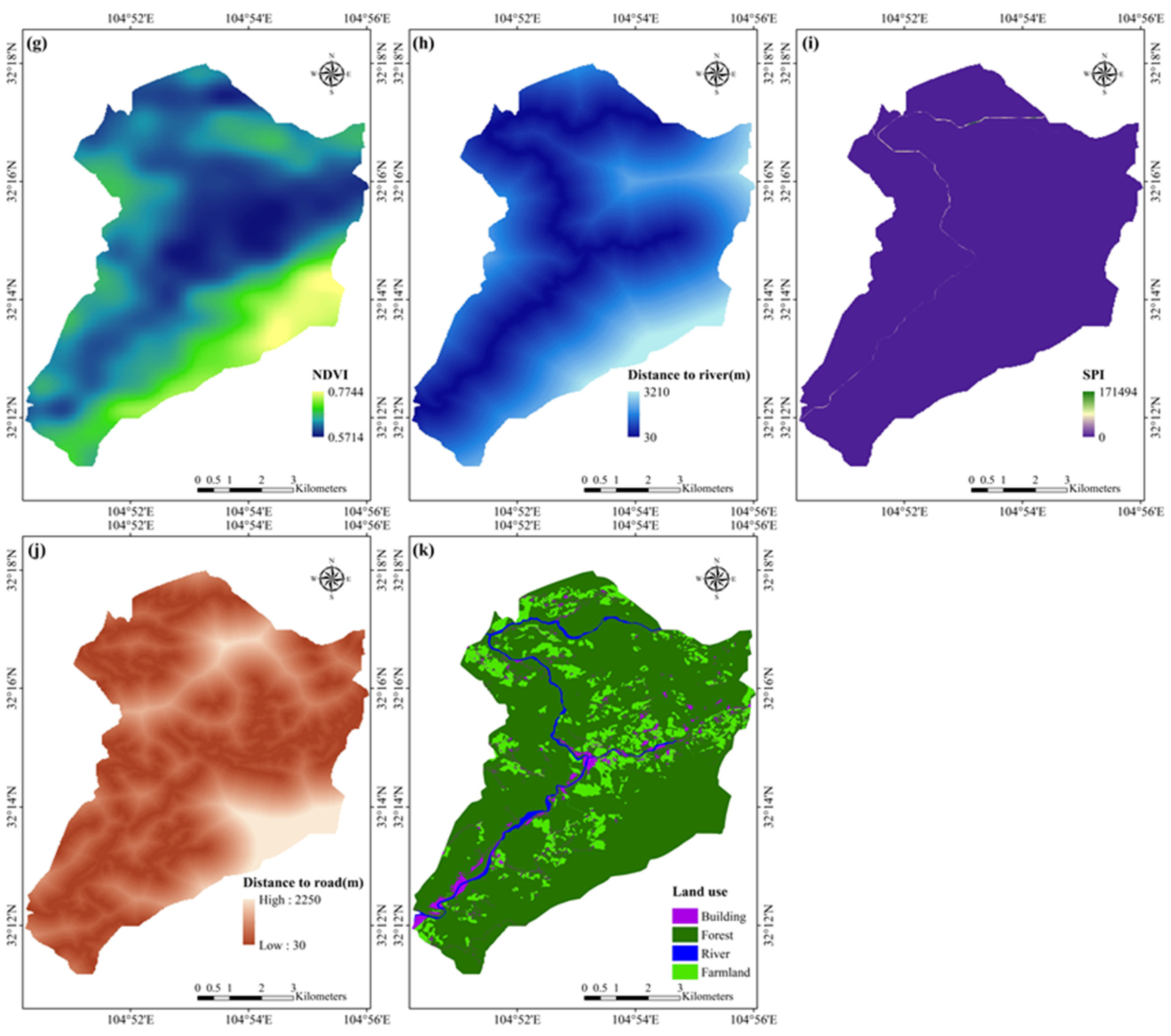
The occurrence of landslides is closely related to environmental factors and artificial factors. To effectively evaluate the landslide susceptibility of the Hongxi River Basin, conditioning factors must be taken into consideration. According to research on the conditions and landslide mechanism in the past few decades, there are many landslide conditioning factors [34,35,36] to choose from. This study selects 11 landslide conditioning factors, which can be divided into three major categories: geological and environmental conditions [37], topography conditions, and human activities conditions [38]. The geological and environmental conditions are related to lithology, normalized difference vegetation index (NDVI), distance to river, and land use. The topography conditions are related to elevation, slope angle, slope aspect, total curvature, surface roughness, and stream power index (SPI). Human activity conditions related to the distance to road (Figure 2). And the NDVI and SPI, are calculated as follows:
N D V I = N I R R N I R + R S P I = S C A × tan S L O P E
where NIR represents the near-infrared band reflectance, and R represents red band reflectance. The SCA is the specific catchment area, and SLOPE is the slope gradient.
Lithology is an important factor related to landslides, different rock types have different properties, which are the basic material conditions for landslides. Elevation, slope angle, slope aspect total curvature, and surface roughness reflect the topographic relief of an area and the smoothness of the surface, which is closely related to the movement and accumulation of landslides. NDVI and land use represent the distribution of land cover and they can affect the degree of loosening of rock and soil, which in turn affects the generation of landslides. SPI represents the erosive ability of water flow, when the river moves, it scours the landscape and may wash away or create deposits [39], which can affect the generation of landslides. So, the SPI and distance to river are also selected as conditioning factors. In recent years, human activities have also had an impact on the geographical environment, and the impact of some projects on the terrain will make the area more prone to landslides. In this study, we use distance to road to represent human activities.
The sources and data format of all conditioning factors data are listed in Table 1 The conditioning factors of landslides have different formats and different spatial resolutions. The data formats include vector data and raster data, and the spatial resolutions are 90 m and 500 m. All conditioning factors data are unified through vector-raster conversion, resampling, and normalization and finally unified to 30 m raster data. To avoid the effect of differences between different data magnitudes on the model, all conditioning factors are normalized to 0–1.

2.3. Method

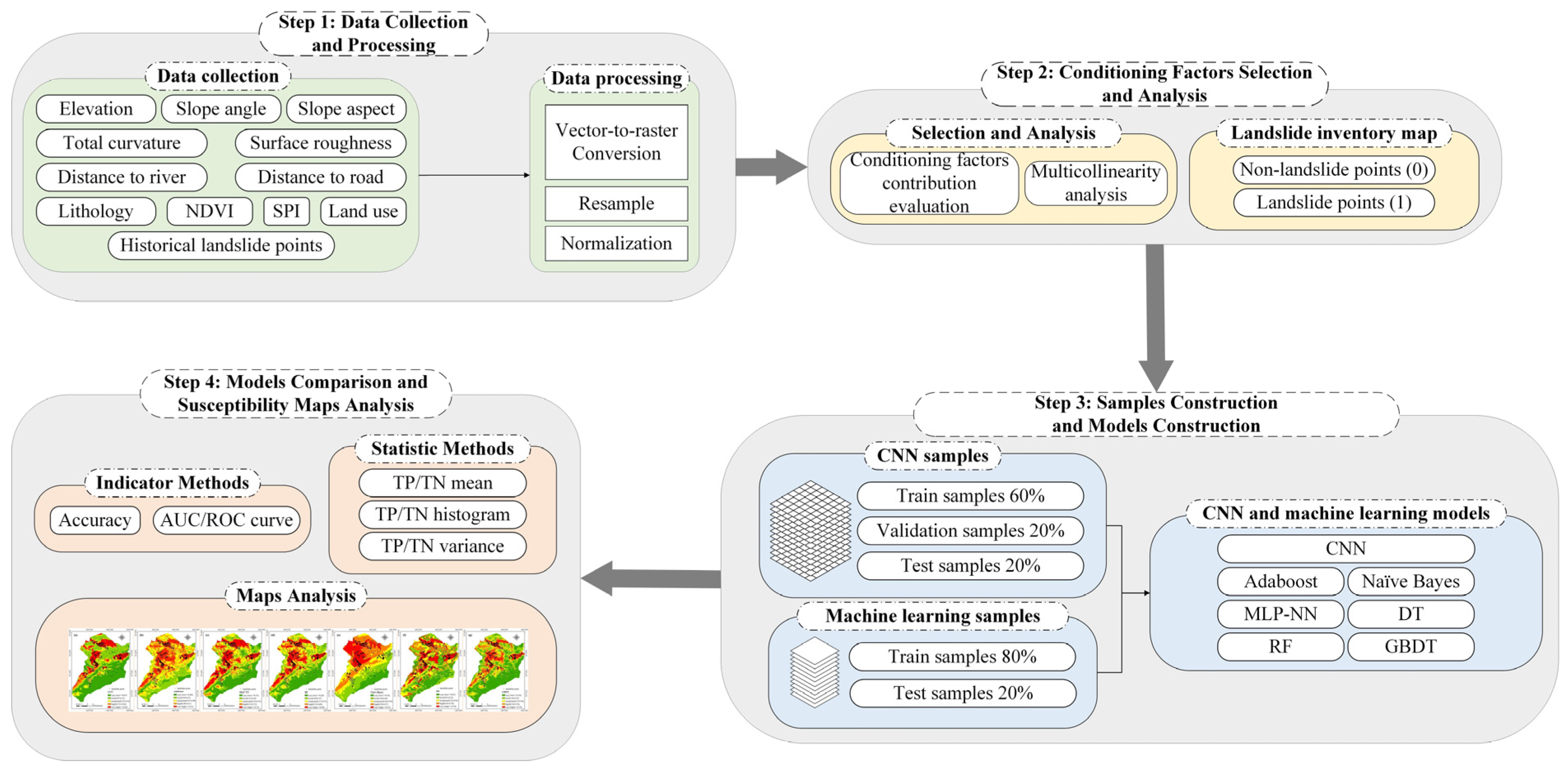
The CNN and six ML methods—Adaboost, naive Bayes, MLP-NN, DT, RF and GBDT are applied to the LSA and their results are compared. The workflow of the LSA is shown in Figure 3 and four steps are described as follows.
(1) All conditioning factors data and history landslide points are collected. These data are unified to the same spatial resolution and format through vector-to-raster conversion, resample and normalization;
(2) Multicollinearity analysis and contribution analysis are used to select and analysis conditioning factors. They can calculate the correlation and contribution rate of each conditioning factor, and determine whether every factor is suitable for LSA. Furthermore, the same number of non-landslide points are generated randomly, then the landslide inventory map is created by combining landslide and non-landslide points;
(3) CNN and ML samples are constructed for model training and testing. For the CNN, samples of 7*7 size are constructed centered on each landslide/non-landslide point, and the samples of 1*1 size are built for machine learning. All samples are divided into train, validation, and test of the ratio 6:2:2 for the CNN, and 8:2 for ML. ML methods used in this study are Adaboost, naive Bayes, MLP-NN, DT, RF and GBDT. All samples are used to train and test the LSA model;
(4) All LSA models are evaluated by the indicator method, statistic method and maps analysis. Indicators used in this study are accuracy, AUC value, and ROC Curve. Statistic methods are represented by the mean, variance, and histogram of TP and TN. Susceptibility maps are made in ArcGIS. Indicator and statistic methods are used to compare the performance and characteristic of the CNN and ML methods, and the maps can represent the spatial distribution difference in the results.

2.3.1. Multicollinearity Analysis and Contribution Rate Analysis

Conditioning factors cannot be directly applied to LSA. Taking into account the possible high correlation between them, it is necessary to select the conditioning factors through multicollinearity analysis. In addition, the contribution rate of each conditioning factor to the landslide is calculated using feature importance ranking in RF.
The possible high linear correlation between conditioning factors will increase the dimensionality of the data, reduce the calculation speed when training and assessing, and may even reduce the final accuracy or make wrong assessment result [39]. Therefore, it is necessary to use multicollinearity analysis [40] to analyze the correlation between the 11 conditioning factors. There are two indicators used to evaluate the correlation, they are tolerance (TOL) and variance inflation factor (VIF). When TOL is greater than 0.1 or VIF is less than 10, there is no strong linear correlation among these factors. The multicollinearity method is achieved via SPSS software.
In addition, it is necessary to consider the contribution rate of each conditioning factor to the landslide. It is achieved by feature importance rank in RF, which is implemented, based on the Gini index. The Gini index represents the probability that a randomly selected sample in the sample set is misclassified [41]. The smaller the Gini index, the purer the sample set. The greater the contribution rate, the greater impact the factor has on the landslide.

2.3.2. CNN

The CNN is the most commonly used DL method [18]. It mainly extracts the information and deep features of the input data through convolution and pooling, and finally achieves classification [42] or regression [43] by matching labels and updating parameters using stochastic gradient descent.
The CNN usually consists of convolution layers, pooling layers, and fully connected layers. The convolution layer not only considers the features of the current position, but also takes into account the features within a certain range of the surrounding neighbors [44]. This is very consistent with the first law of geography, that is, everything is related to everything else, but things that are near each other, are more related to each other [45], which is also the reason why the CNN performs well in many geographic problems. Then, the pooling layers further extract the important information from the features extracted by the convolution layers [46]. The fully connected layers [47] finally stretch the deep features after convolution and pooling. It corresponds to the label of the samples and finally determines the mapping relationship between samples and labels by updating the weight within the network.
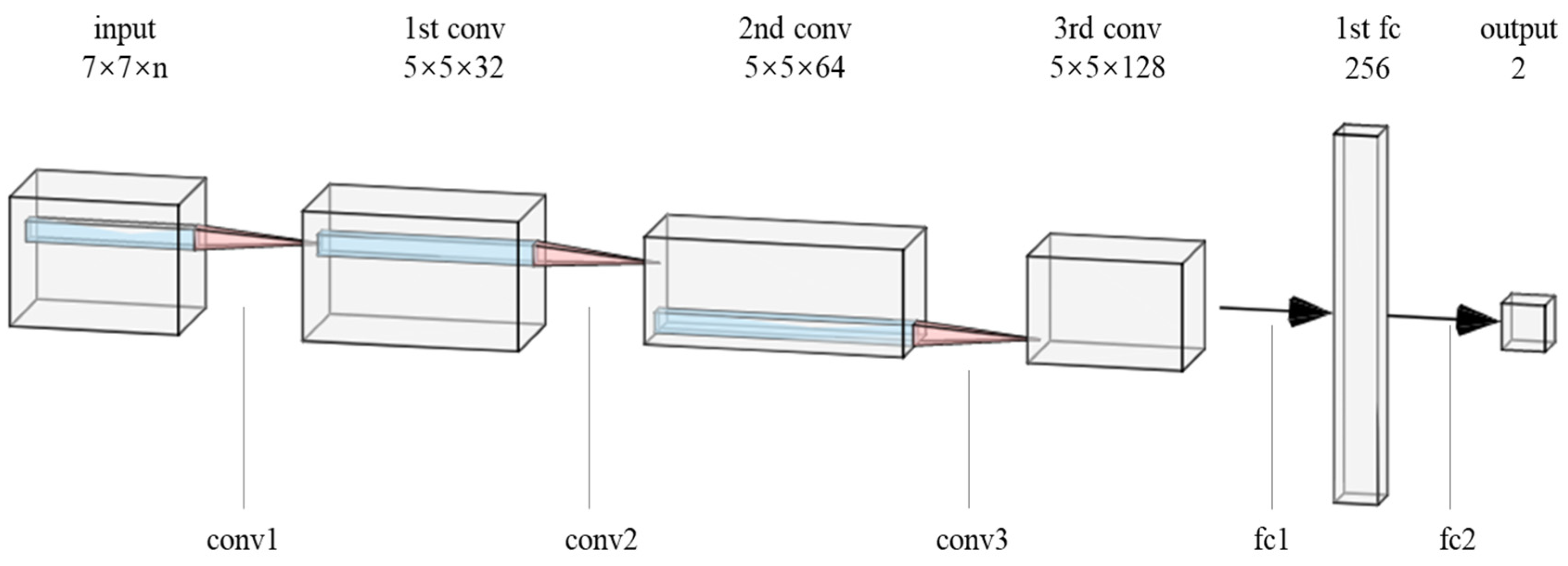
In the process of the development of the CNN, some excellent network structures have been produced [18,19]. The CNN structure referenced in this study is AlexNet [17]. AlexNet has the following characteristics: (1) data augmentation is used; (2) ReLU function is employed as the activation function [48]; (3) dropout is utilized to prevent overfitting [49]; (4) overlapping pooling is used; (5) multiple GPUs are used for training. Based on the above, in this study, AlexNet is employed to build a CNN model suitable for the LSA in the study area.

2.3.3. Adaboost

Adaboost is an iterative algorithm. Its core idea is to train multiple weak classifiers through multiple iterations and finally form a strong classifier [50]. In the process of each iteration, the new weak classifier will pay attention to the data samples that the previous classifier misclassified, and the parameters are updated. Each weak classifier focuses on a part of the data in the dataset, so when the weak classifiers are combined, the result will be a strong classifier [51]. In the final judgment of the category, it is necessary to perform weighted voting, according to the weight of each weak classifier.

2.3.4. MLP-NN

The MLP-NN is the simplest neural network structure. It only contains three network structures: the input layer, hidden layer, and output layer [52]. Each layer of the network is fully connected. Each neuron uses a linear activation function to calculate the value, and the weight is continuously updated through training to obtain the final result [53]. The greatest advantage of the MLP-NN is its simple structure and fast calculation speed, but because the network uses a linear activation function, overfitting can easily occur.

2.3.5. RF

RF is a classifier composed of multiple trees for the training and prediction of samples [54]. The core of RF is to randomly select multiple sets of features from the dataset and build a decision tree for each set of features. Then, the final classification result is obtained by voting according to the judgment result of each decision tree. Compared with other methods, the RF has several advantages. First, because of its randomness when selecting samples and features, the RF is not prone to overfitting. RF can also obtain the contribution rate of each input feature [41]. In addition, the RF has a faster calculation speed, which is superior to DL.

2.3.6. Naive Bayes

Naive Bayes is a classification method, based on the Bayes theorem and the independence assumption of the feature conditions [55]. The core of naive Bayes is to calculate category probabilities and conditional probabilities from the input training data. Then, the Bayes theorem is used to make predictions about the new data [56]. Naive Bayes is based on the input joint probability distribution between the feature and the output label, and then the result is obtained according to the concept of conditional probability. The naive Bayes method is very simple and intuitive, easy to understand, and easy to implement.

2.3.7. DT

DT uses a hierarchical structure from the top to the bottom of the tree, and the final prediction is achieved through nodes at different levels [57]. Its basic principle is that starting from the root node of the tree, a certain characteristic value of the input is judged, and a threshold is generated. The judgment result is divided into two leaf nodes, according to the threshold, and then the leaf node is used to attain a certain characteristic value [58]. This process goes back and forth, and finally, a tree structure that can judge the data is generated.

2.3.8. GBDT

GBDT is an integrated model, based on regression trees and gradient iteration as the framework [59]. Its core idea is to generate a residual regression tree for each iteration, and each regression tree learns the results and residuals of all previous trees. Finally, a gradient boosting tree is generated by accumulating the regression tree generated in each iteration, and finally, the classification function is realized [60]. GBDT is a complex method that is more suitable for low-dimensional data. When dealing with high-dimensional data, it is usually necessary to carefully adjust the parameters to obtain better results. This method takes longer than other ML methods when training and predicting.

2.3.9. Samples Construction

To train the LSA model, it is necessary to construct training samples, validation samples, and test samples. The training samples are used to train and evaluate the model, the validation samples are used to verify the training results during the training process, and the test samples are used to evaluate models. The construction of the CNN model samples and ML model samples is different. The CNN considers the information around landslide/non-landslide points. The landslide/non-landslide point is the center of the 7*7 window size, and the information of 11 conditioning factors is extracted to form a 7*7*11 sample. The window size of the input data is determined, based on the area size of the study area and multiple tests. Each sample is labeled, and landslide/non-landslide points are marked 1/0. For six ML samples, only 11 conditioning factors of landslide/non-landslide points need to be extracted to construct a 1*1*11 sample, which is also labeled 1/0.
Once the sample construction is completed, for the CNN, the landslide samples and non-landslide samples are randomly divided into training samples, validation samples, and test samples at a ratio of 6:2:2. For the six ML methods, the landslide/non-landslide samples are randomly divided according to an 8:2 ratio [61].

2.3.10. Models Construction

In this research, the CNN, AdaBoost, MLP-NN, RF, naive Bayes, DT, and GBDT models are constructed. The structure and parameters of the CNN are adjusted to be suitable to the study area. The structure of the CNN is shown in Figure 4 and the parameters are shown in Table 2. Six ML models are constructed via the scikit-learn package using Python language. These models have been adjusted many times and performed well on the training samples.

3. Results

This section first shows the result of multicollinearity analysis and contribution rate analysis. Then, the result of the indicator method, statistical methods, and LSMs are shown. Finally, the performance and characteristics of these methods are compared and discussed.

3.1. Analysis of the Conditioning Factors

The results (Table 3) show that the VIFs of the 11 conditioning factors are all less than 10, and the TOLs are all greater than 0.1, which means all of these conditioning factors are independent and can be used for the LSA.
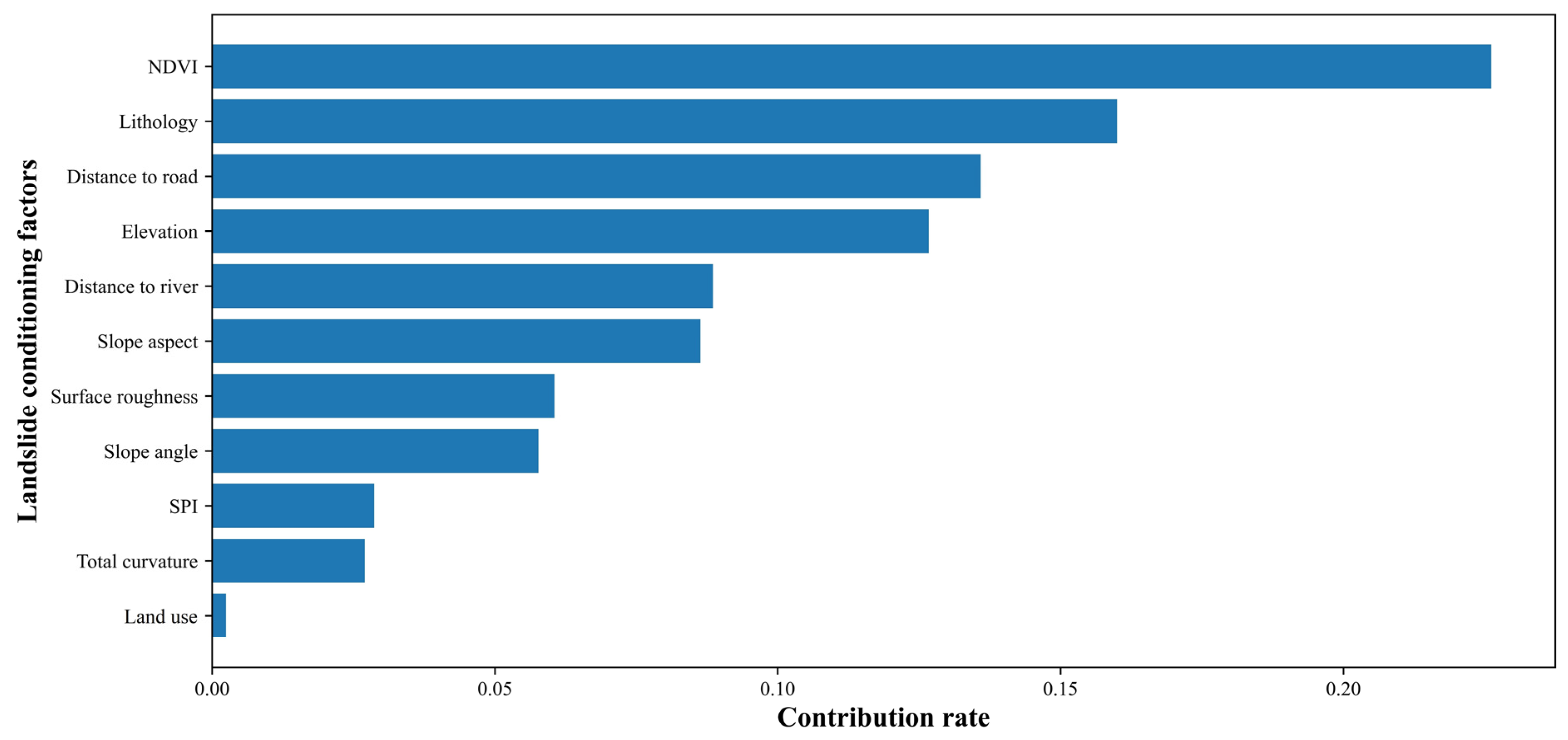
By contribution analysis, Figure 5 shows that the NDVI, lithology, distance to road, and elevation have the greatest influence on the landslide, which shows that the local rock and soil properties, geological structure, topography, and human activities have a relatively important impact on the landslide. Land use has the least impact on landslides, which is related to the small difference in land use spatial distribution. Most of the land use in the study area is forestland, so the impact of land use on local landslides is minimal. From Figure 2, it can be found that landslides mostly occur in areas with NDVI values less than 0.65, especially 0.6–0.65, very few landslides occur in areas with NDVI values greater than 0.65. This means the differences in NDVI have a large effect on landslides, so the contribution of the NDVI is the highest among all conditioning factors.

3.2. LSMs

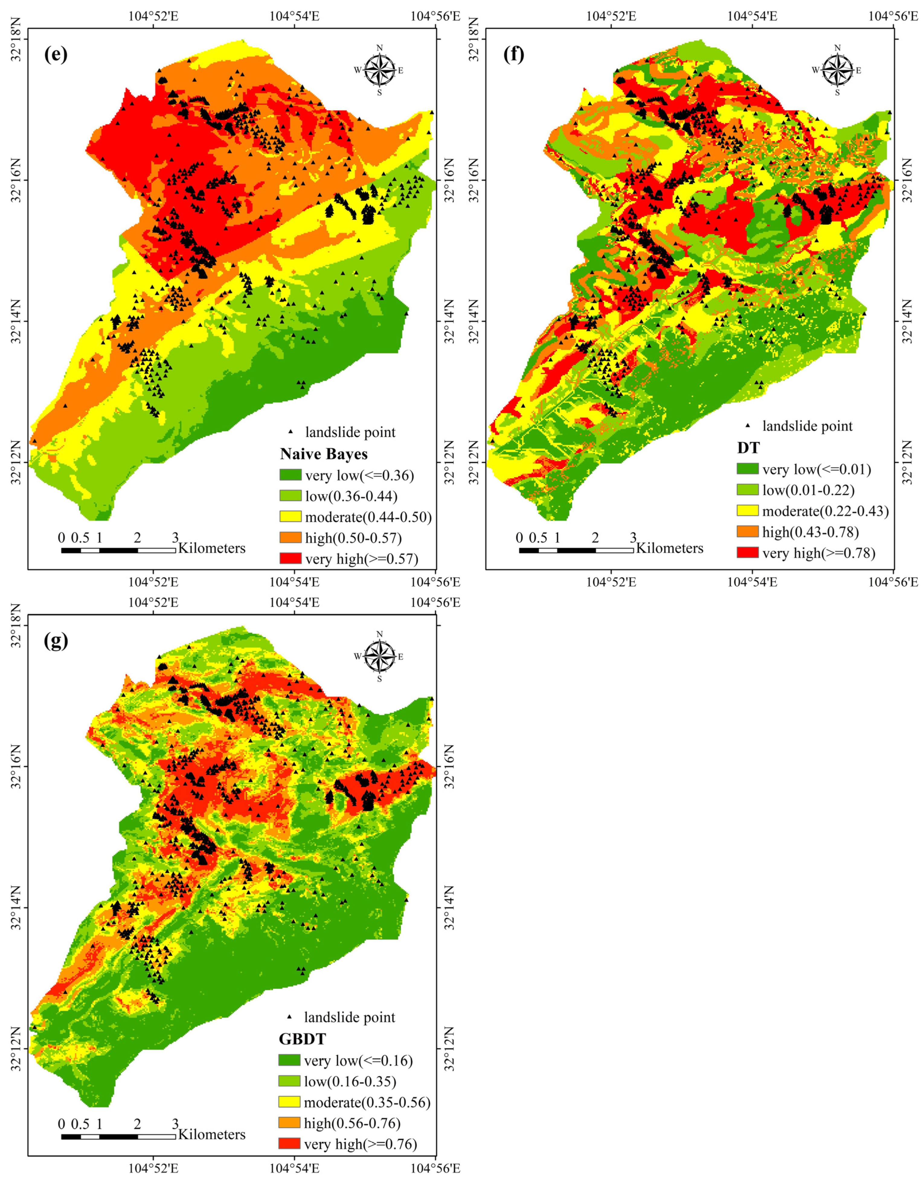
LSMs are made to analyze the differences and characteristics between the CNN and six ML models from the perspective of spatial distribution. The natural break method is used to classify the susceptibility levels and the maps are shown in Figure 6. It can be seen from the LSMs that all methods can identify most of the landslide points. The LSM of the CNN is more concentrated on the very high and very low susceptibility, and the ML methods have high, moderate, and low levels. The CNN cannot identify some scattered landslide points in the study area, while other ML methods can. This may be related to the convolution operation in the CNN. The convolutional operation takes into account the surrounding information of the ground feature. This is its advantage in geography, but it may also be its disadvantage. In areas with a high frequency of landslides, the surrounding environment is prone to cause landslides, and landslide information is highlighted and strengthened. This phenomenon will make the CNN judgment of landslide points more accurate and certain, but for scattered landslide occurrence points, the surrounding environment does not easily cause landslides, so through the convolution operation, it is possible to weaken the conditioning factors information and make it difficult to identify landslide points. These scattered landslide points need to be considered in the actual disaster prevention and mitigation.

3.3. Method Comparison

The method comparison uses the indicator method and statistical method. The indicators used in the indicator method are the accuracy, area under curve (AUC), and ROC curves [10,22,62]. The accuracy is the proportion of the number of correctly discriminated samples to the total number of test samples; the larger the value, the higher the accuracy of the model. The AUC represents the area under the ROC curve; the closer the value is to 1, the better the evaluation result of the model. The accuracy is calculated as follows:
a c c u r a c y = T P + T N T P + T N + F P + F N
where TP is true positive samples, TN is true negative samples, FP is false positive samples, and FN is false negative samples.
The results are shown in Figure 7 and Table 4. The results show that the accuracy and AUC of the CNN are the highest among all models, which can explain how the CNN outperforms other ML methods. The performance of GBDT is better than other ML methods and it is close to the CNN. The MLP-NN and the naive Bayes cannot obtain a good accuracy and AUC, as other methods.
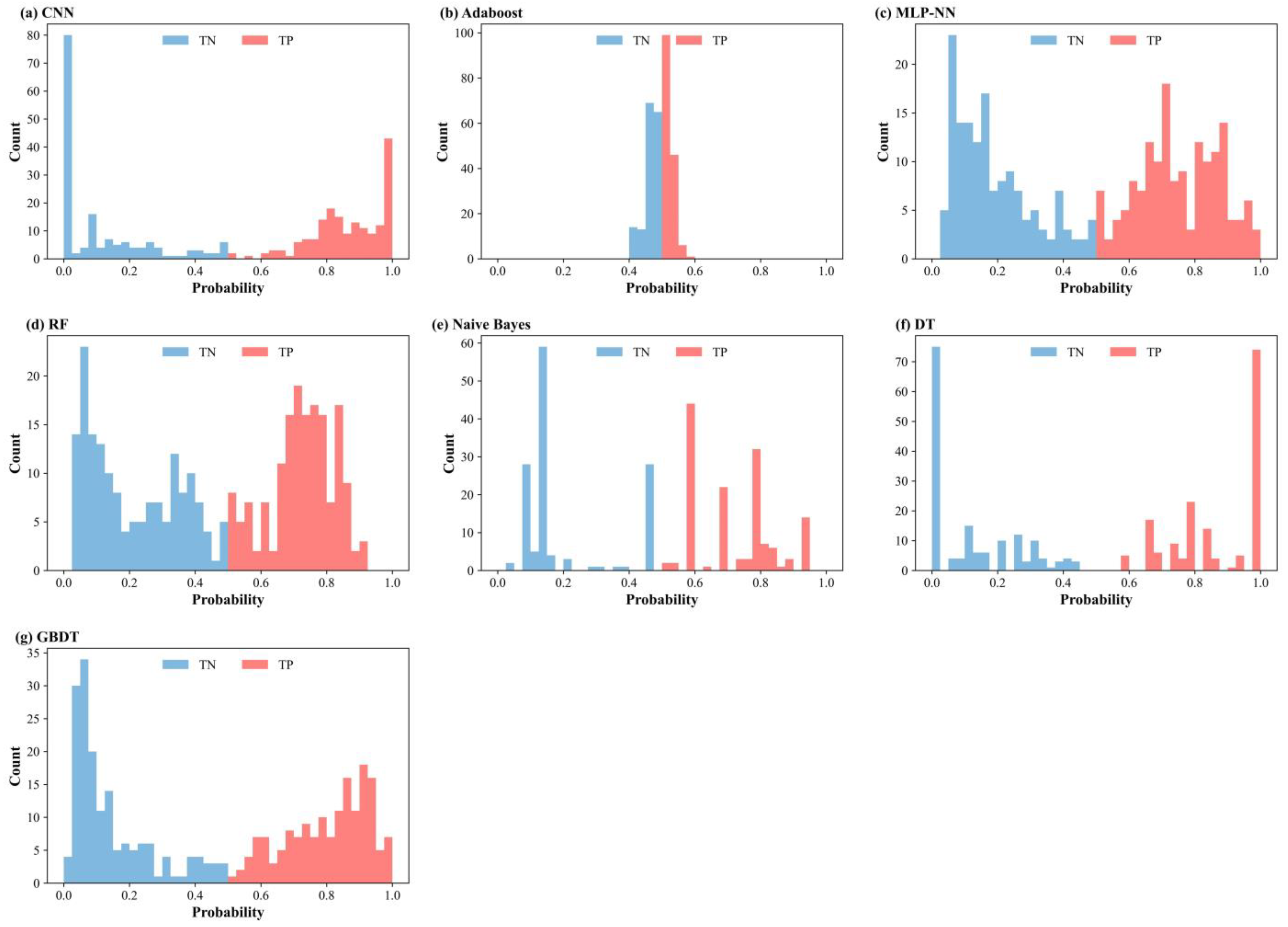
The statistical method focuses on the two types that are correctly identified in the test sample, that is, positive samples that are discriminated as positive, and negative samples that are discriminated as negative, they are the TP samples and TN samples correspondingly. The histograms of the probabilities of the TP and TN samples are visualized and their mean and variance are calculated. The results are shown in Table 4 and Figure 8. It can be seen from the results that the TP-mean/TN-mean of the CNN is the highest/smallest among all methods. This indicates that the CNN product is more certain about the landslide/non-landslide judgment in the LSA problem. Comparing the variance of the probability evaluated by the CNN and other methods, it can be seen that the TP-variance and TN-variance of the CNN are very small, which shows that its judgment results are both definite and concentrated. It should be noted that the variance obtained by the AdaBoost method is smaller than that of the CNN, but from the histogram, it can be seen that the probability value of its judgment of a landslide/non-landslide, is approximately 0.5, which is not certain about its judgment of landslides.

4. Discussion

The result shows that the CNN has a better performance than ML methods when used in the LSA. However, some results need to be discussed and there are still several shortcomings in this study that need to be improved upon in the future.
From the LSM of the CNN, the landslide cluster region can be identified more clearly. At present, a CNN has a fixed detection range for the surrounding environmental information of the landslide points. This is one of the reasons why the information on disaster scatter points is easily weakened. So in the future, it may be possible to dynamically adjust the convolution kernel size according to the degree of landslide points cluster. This is a direction of improving the accuracy of the LSA.
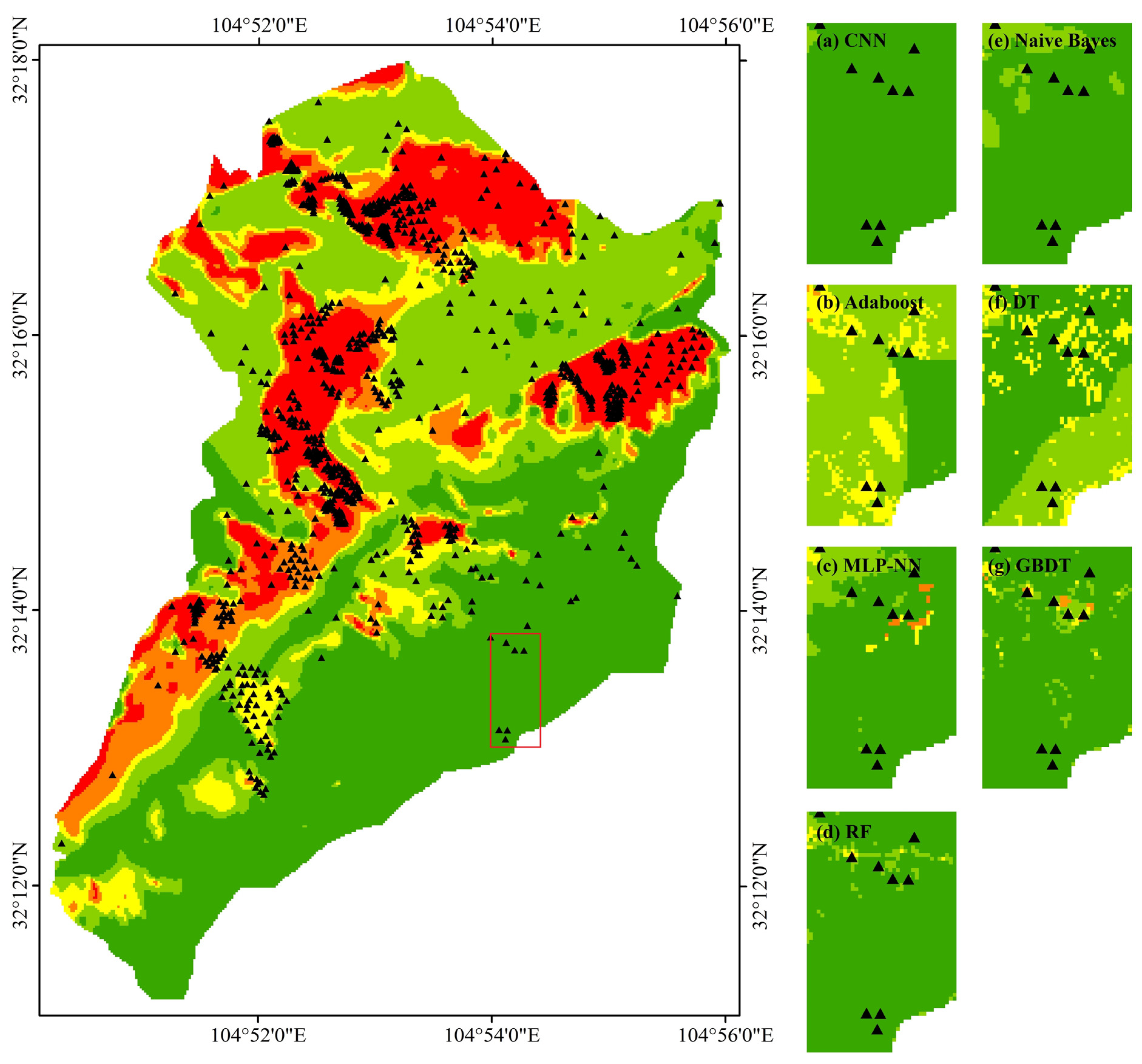
In addition, it can be seen from the figure that whether it is a CNN or ML method, it is difficult to identify landslides in the southeastern part of the study area Figure 9. Most of these points are located at relatively high altitudes and are relatively scattered. Although the frequency of landslides in this area is relatively low, more attention should be given to these landslides for the prevention and control of disasters. Humans always pay more attention to areas with a high frequency of landslides. The experience and methods of prevention and control are also richer in these areas than in areas with a low frequency of landslides. This is related to the different distribution of conditioning factors between the cluster landslide points and scattered landslide points, which is not studied in-depth in this paper and needs to be studied in the future.

5. Conclusions

In this study, the CNN and six ML methods are compared in the LSA, and the characteristics of the CNN model and its differences with other ML methods are further studied through its performance in the LSA of the Hongxi River Basin in Pingwu County, Mianyang City, Sichuan Province, China. Based on the landslide points collected in the study area and the surrounding environment, 11 landslide conditioning factors are selected, and the correlation degree among each factor and their influence on the landslide are analyzed through a multicollinearity analysis and contribution rate analysis. Subsequently, the CNN model and six ML models are trained and constructed. Finally, an indicator method and statistic method are used to analyze the characteristics and differences between the CNN and ML methods.
It can be seen from the model comparison results of the model that the performance of the CNN is better than the other six ML methods, in terms of accuracy (86.41%), AUC (0.9249). Moreover, from the histogram distribution, the mean, and variance of the TP and TN samples, it can be seen that the prediction probability of the CNN is more concentrated than that of ML methods and it is more certain about its result. From the spatial distribution of the LSMs, the landslide susceptibility predicted by the CNN is more clustered, especially in the areas where the landslide points are relatively clustered. However, the other six ML methods only consider the information of the current landslide point without considering the environmental information around the disaster point, which also makes their LSMs’ aggregation phenomenon not obvious. The high accuracy and concentration of the CNN are significant for disaster prevention and mitigation, because of the more specific very high susceptibility area, human, and material resources that can be used efficiently.
There are still some limitations in this study that need to be improved. The results show that the CNN performs better at landslide cluster areas than scatter areas. Dynamic convolution might work for this problem and this will be further explored in future research. It can also be seen from the LSMs that there are some landslide points in the southeastern area of the study area, but the CNN model and most ML models do not mark this area as a high/very high susceptibility area. So in the future, this phenomenon can be further improved.

Author Contributions

Conceptualization, M.W. and K.L.; methodology, Z.J.; software, Z.J.; validation, Z.J.; writing, draft preparation, review and editing, Z.J. All authors have read and agreed to the published version of the manuscript.

Funding

This research was funded by the National Key Research and Development Plan (2017YFC1502902). The financial support is highly appreciated.

Data Availability Statement

Not applicable.

Conflicts of Interest

The authors declare no conflict of interest.

References

  1. Leynaud, D.; Mulder, T.; Hanquiez, V.; Gonthier, E.; Régert, A. Sediment Failure Types, Preconditions and Triggering Factors in the Gulf of Cadiz. Landslides 2017, 14, 233–248. [Google Scholar] [CrossRef]
  2. Chang, J.-M.; Chen, H.; Jou, B.J.-D.; Tsou, N.-C.; Lin, G.-W. Characteristics of Rainfall Intensity, Duration, and Kinetic Energy for Landslide Triggering in Taiwan. Eng. Geol. 2017, 231, 81–87. [Google Scholar] [CrossRef]
  3. Chowdhuri, I.; Pal, S.C.; Chakrabortty, R.; Malik, S.; Das, B.; Roy, P. Torrential Rainfall-Induced Landslide Susceptibility Assessment Using Machine Learning and Statistical Methods of Eastern Himalaya. Nat. Hazards 2021, 107, 697–722. [Google Scholar] [CrossRef]
  4. Tang, Y.; Che, A.; Cao, Y.; Zhang, F. Risk Assessment of Seismic Landslides Based on Analysis of Historical Earthquake Disaster Characteristics. Bull. Eng. Geol. Environ. 2020, 79, 2271–2284. [Google Scholar] [CrossRef]
  5. Klose, M.; Maurischat, P.; Damm, B. Landslide Impacts in Germany: A Historical and Socioeconomic Perspective. Landslides 2016, 13, 183–199. [Google Scholar] [CrossRef]
  6. Gariano, S.L.; Sarkar, R.; Dikshit, A.; Dorji, K.; Brunetti, M.T.; Peruccacci, S.; Melillo, M. Automatic Calculation of Rainfall Thresholds for Landslide Occurrence in Chukha Dzongkhag, Bhutan. Bull. Eng. Geol. Environ. 2019, 78, 4325–4332. [Google Scholar] [CrossRef]
  7. Vilceanu, C.B.; Herban, I.S.; Grecea, C. Geodetic Studies with Significant Contribution to Landslide Monitoring in South-Western Romania—Area with High Risk Potential. Teh. Vjesn. 2016, 23, 1623–1630. [Google Scholar] [CrossRef] [Green Version]
  8. Huang, R.; Pei, X.; Fan, X.; Zhang, W.; Li, S.; Li, B. The Characteristics and Failure Mechanism of the Largest Landslide Triggered by the Wenchuan Earthquake, May 12, 2008, China. Landslides 2012, 9, 131–142. [Google Scholar] [CrossRef]
  9. Nguyen, B.-Q.-V.; Kim, Y.-T. Regional-Scale Landslide Risk Assessment on Mt. Umyeon Using Risk Index Estimation. Landslides 2021, 18, 2547–2564. [Google Scholar] [CrossRef]
  10. Nhu, V.-H.; Mohammadi, A.; Shahabi, H.; Bin Ahmad, B.; Al-Ansari, N.; Shirzadi, A.; Clague, J.J.; Jaafari, A.; Chen, W.; Nguyen, H. Landslide Susceptibility Mapping Using Machine Learning Algorithms and Remote Sensing Data in a Tropical Environment. Int. J. Environ. Res. Public Health 2020, 17, 4933. [Google Scholar] [CrossRef]
  11. Sano, H.; Usuda, Y.; Iwai, I.; Taguchi, H.; Misumi, R.; Hayashi, H. Generation of Risk Information Based on Comprehensive Real-Time Analysis of Flooding and Landslide Disaster Occurrence Hazard and Social Vulnerability. J. Disaster Res. 2020, 12, 676–687. [Google Scholar] [CrossRef]
  12. Wang, B.; Ding, M.; Li, S.; Liu, L.; Ai, J. Assessment of Landscape Ecological Risk for a Cross-Border Basin: A Case Study of the Koshi River Basin, Central Himalayas. Ecol. Indic. 2020, 117, 106621. [Google Scholar] [CrossRef]
  13. Abedini, M.; Tulabi, S. Assessing LNRF, FR, and AHP Models in Landslide Susceptibility Mapping Index: A Comparative Study of Nojian Watershed in Lorestan Province, Iran. Environ. Earth Sci. 2018, 77, 405. [Google Scholar] [CrossRef]
  14. Acharya, T.D.; Lee, D.H. Landslide Susceptibility Mapping Using Relative Frequency and Predictor Rate along Araniko Highway. KSCE J. Civ. Eng. 2019, 23, 14. [Google Scholar] [CrossRef]
  15. Abidi, A.; Demehati, A.; El Qandil, M. Landslide Susceptibility Assessment Using Evidence Belief Function and Frequency Ratio Models in Taounate City (North of Morocco). Geotech. Geol. Eng. 2019, 37, 5457–5471. [Google Scholar] [CrossRef]
  16. Wang, Q.; Li, W.; Wu, Y.; Pei, Y.; Xie, P. Application of Statistical Index and Index of Entropy Methods to Landslide Susceptibility Assessment in Gongliu (Xinjiang, China). Environ. Earth Sci. 2016, 75, 599. [Google Scholar] [CrossRef]
  17. Krizhevsky, A.; Sutskever, I.; Hinton, G.E. ImageNet Classification with Deep Convolutional Neural Networks. Commun. ACM 2017, 60, 84–90. [Google Scholar] [CrossRef] [Green Version]
  18. Lecun, Y.; Bottou, L.; Bengio, Y.; Haffner, P. Gradient-Based Learning Applied to Document Recognition. Proc. IEEE 1998, 86, 2278–2324. [Google Scholar] [CrossRef] [Green Version]
  19. Shi, X.; Chen, Z.; Wang, H.; Yeung, D.-Y.; Wong, W.; Woo, W. Convolutional LSTM Network: A Machine Learning Approach for Precipitation Nowcasting. In Proceedings of the Advances in Neural Information Processing Systems 28 (NIPS 2015), Montreal, QC, Canada, 7–12 December 2015; Cortes, C., Lawrence, N.D., Lee, D.D., Sugiyama, M., Garnett, R., Eds.; Neural Information Processing Systems (NIPS): La Jolla, CA, USA, 2015; Volume 28. [Google Scholar]
  20. Seaman, W.; Yavuz, S. Image Visual Sensor Used in Health-Care Navigation in Indoor Scenes Using Deep Reinforcement Learning (DRL) and Control Sensor Robot for Patients Data Health Information. J. Med. Imaging Health Inform. 2021, 11, 104–113. [Google Scholar] [CrossRef]
  21. Zou, Z.; Zhu, T.; Xu, L.; Luo, A.-L. Celestial Spectra Classification Network Based on Residual and Attention Mechanisms. Publ. Astron. Soc. Pac. 2020, 132, 044503. [Google Scholar] [CrossRef]
  22. Zhang, G.; Wang, M.; Liu, K. Forest Fire Susceptibility Modeling Using a Convolutional Neural Network for Yunnan Province of China. Int. J. Disaster Risk Sci. 2019, 10, 386–403. [Google Scholar] [CrossRef] [Green Version]
  23. LeCun, Y.; Bengio, Y.; Hinton, G. Deep Learning. Nature 2015, 521, 436–444. [Google Scholar] [CrossRef]
  24. Ma, X.; Tao, Z.; Wang, Y.; Yu, H.; Wang, Y. Long Short-Term Memory Neural Network for Traffic Speed Prediction Using Remote Microwave Sensor Data. Transp. Res. Part C Emerg. Technol. 2015, 54, 187–197. [Google Scholar] [CrossRef]
  25. Liu, W.; Wang, Z.; Liu, X.; Zeng, N.; Liu, Y.; Alsaadi, F.E. A Survey of Deep Neural Network Architectures and Their Applications. Neurocomputing 2017, 234, 11–26. [Google Scholar] [CrossRef]
  26. Chen, L.; Cao, Y.; Ma, L.; Zhang, J. A Deep Learning-Based Methodology for Precipitation Nowcasting with Radar. Earth Space Sci. 2020, 7, e2019EA000812. [Google Scholar] [CrossRef] [Green Version]
  27. Saha, S.; Saha, A.; Hembram, T.K.; Pradhan, B.; Alamri, A.M. Evaluating the Performance of Individual and Novel Ensemble of Machine Learning and Statistical Models for Landslide Susceptibility Assessment at Rudraprayag District of Garhwal Himalaya. Appl. Sci. 2020, 10, 3772. [Google Scholar] [CrossRef]
  28. Cai, H.; Chen, T.; Niu, R.; Plaza, A. Landslide Detection Using Densely Connected Convolutional Networks and Environmental Conditions. IEEE J. Sel. Top. Appl. Earth Obs. Remote Sens. 2021, 14, 5235–5247. [Google Scholar] [CrossRef]
  29. Richman, M.B.; Leslie, L.M. Adaptive Machine Learning Approaches to Seasonal Prediction of Tropical Cyclones. Procedia Comput. Sci. 2012, 12, 276–281. [Google Scholar] [CrossRef] [Green Version]
  30. Arabameri, A.; Saha, S.; Roy, J.; Chen, W.; Blaschke, T.; Tien Bui, D. Landslide Susceptibility Evaluation and Management Using Different Machine Learning Methods in The Gallicash River Watershed, Iran. Remote Sens. 2020, 12, 475. [Google Scholar] [CrossRef] [Green Version]
  31. Chen, W.; Peng, J.; Hong, H.; Shahabi, H.; Pradhan, B.; Liu, J.; Zhu, A.-X.; Pei, X.; Duan, Z. Landslide Susceptibility Modelling Using GIS-Based Machine Learning Techniques for Chongren County, Jiangxi Province, China. Sci. Total Environ. 2018, 626, 1121–1135. [Google Scholar] [CrossRef]
  32. Hong, H.; Liu, J.; Bui, D.T.; Pradhan, B.; Acharya, T.D.; Pham, B.T.; Zhu, A.-X.; Chen, W.; Ahmad, B.B. Landslide Susceptibility Mapping Using J48 Decision Tree with AdaBoost, Bagging and Rotation Forest Ensembles in the Guangchang Area (China). Catena 2018, 163, 399–413. [Google Scholar] [CrossRef]
  33. Li, C.; Wang, M.; Liu, K. Identification of Landslides and Debris Flows Using Semi-Variance Model: A Case Study of Hongxi Basin in Sichuan. Geogr. Geo-Inf. Sci. 2019, 35, 47–52. [Google Scholar]
  34. Di Napoli, M.; Marsiglia, P.; Di Martire, D.; Ramondini, M.; Ullo, S.L.; Calcaterra, D. Landslide Susceptibility Assessment of Wildfire Burnt Areas through Earth-Observation Techniques and a Machine Learning-Based Approach. Remote Sens. 2020, 12, 2505. [Google Scholar] [CrossRef]
  35. Kadavi, P.R.; Lee, C.-W.; Lee, S. Application of Ensemble-Based Machine Learning Models to Landslide Susceptibility Mapping. Remote Sens. 2018, 10, 1252. [Google Scholar] [CrossRef] [Green Version]
  36. Hong, H.; Pourghasemi, H.R.; Pourtaghi, Z.S. Landslide Susceptibility Assessment in Lianhua County (China): A Comparison between a Random Forest Data Mining Technique and Bivariate and Multivariate Statistical Models. Geomorphology 2016, 259, 105–118. [Google Scholar] [CrossRef]
  37. Xie, P.; Wen, H.; Ma, C.; Baise, L.G.; Zhang, J. Application and Comparison of Logistic Regression Model and Neural Network Model in Earthquake-Induced Landslides Susceptibility Mapping at Mountainous Region, China. Geomat. Nat. Hazards Risk 2018, 9, 501–523. [Google Scholar] [CrossRef] [Green Version]
  38. Sun, D.; Wen, H.; Wang, D.; Xu, J. A Random Forest Model of Landslide Susceptibility Mapping Based on Hyperparameter Optimization Using Bayes Algorithm. Geomorphology 2020, 362, 107201. [Google Scholar] [CrossRef]
  39. Chen, X.; Chen, W. GIS-Based Landslide Susceptibility Assessment Using Optimized Hybrid Machine Learning Methods. Catena 2021, 196, 104833. [Google Scholar] [CrossRef]
  40. Tien Bui, D.; Tuan, T.A.; Klempe, H.; Pradhan, B.; Revhaug, I. Spatial Prediction Models for Shallow Landslide Hazards: A Comparative Assessment of the Efficacy of Support Vector Machines, Artificial Neural Networks, Kernel Logistic Regression, and Logistic Model Tree. Landslides 2016, 13, 361–378. [Google Scholar] [CrossRef]
  41. Menze, B.H.; Kelm, B.M.; Masuch, R.; Himmelreich, U.; Bachert, P.; Petrich, W.; Hamprecht, F.A. A Comparison of Random Forest and Its Gini Importance with Standard Chemometric Methods for the Feature Selection and Classification of Spectral Data. BMC Bioinform. 2009, 16, 213. [Google Scholar] [CrossRef] [Green Version]
  42. Shin, H.-C.; Roth, H.R.; Gao, M.; Lu, L.; Xu, Z.; Nogues, I.; Yao, J.; Mollura, D.; Summers, R.M. Deep Convolutional Neural Networks for Computer-Aided Detection: CNN Architectures, Dataset Characteristics and Transfer Learning. IEEE Trans. Med. Imaging 2016, 35, 1285–1298. [Google Scholar] [CrossRef] [PubMed]
  43. Xie, Y.; Xing, F.; Kong, X.; Su, H.; Yang, L. Beyond Classification: Structured Regression for Robust Cell Detection Using Convolutional Neural Network. In Proceedings of the Medical Image Computing and Computer-Assisted Intervention—MICCAI 2015; Navab, N., Hornegger, J., Wells, W.M., Frangi, A.F., Eds.; Springer International Publishing: Cham, Switzerland, 2015; pp. 358–365. [Google Scholar]
  44. Zeng, X.; Wen, S.; Zeng, Z.; Huang, T. Design of Memristor-Based Image Convolution Calculation in Convolutional Neural Network. Neural Comput. Appl. 2018, 30, 503–508. [Google Scholar] [CrossRef]
  45. Sui, D.Z. Tobler’s First Law of Geography: A Big Idea for a Small World? Ann. Assoc. Am. Geogr. 2004, 94, 269–277. [Google Scholar] [CrossRef]
  46. Tran, D.; Bourdev, L.; Fergus, R.; Torresani, L.; Paluri, M. Learning Spatiotemporal Features with 3D Convolutional Networks. In Proceedings of the 2015 IEEE International Conference on Computer Vision (ICCV), Santiago, Chile, 7–13 December 2015; pp. 4489–4497. [Google Scholar]
  47. Long, J.; Shelhamer, E.; Darrell, T. Fully Convolutional Networks for Semantic Segmentation. In Proceedings of the 2015 IEEE Conference on Computer Vision and Pattern Recognition (CVPR), Boston, MA, USA, 7–12 June 2015; pp. 3431–3440. [Google Scholar]
  48. Xu, L.; Choy, C.-S.; Li, Y.-W. Deep Sparse Rectifier Neural Networks for Speech Denoising. In Proceedings of the 2016 IEEE International Workshop on Acoustic Signal Enhancement (IWAENC), Xi’an, China, 13–16 September 2016; 2016. [Google Scholar]
  49. Mendenhall, J.; Meiler, J. Improving Quantitative Structure–Activity Relationship Models Using Artificial Neural Networks Trained with Dropout. J. Comput. Aided Mol. Des. 2016, 30, 177–189. [Google Scholar] [CrossRef] [Green Version]
  50. Schapire, R.; Singer, Y. BoosTexter: A Boosting-Based System for Text Categorization. Mach. Learn. 2000, 39, 135–168. [Google Scholar] [CrossRef] [Green Version]
  51. Wu, Y.; Ke, Y.; Chen, Z.; Liang, S.; Zhao, H.; Hong, H. Application of Alternating Decision Tree with AdaBoost and Bagging Ensembles for Landslide Susceptibility Mapping. Catena 2020, 187, 104396. [Google Scholar] [CrossRef]
  52. Delshadpour, S. Improved MLP Neural Network as Chromosome Classifier. In Proceedings of the IEEE EMBS Asian-Pacific Conference on Biomedical Engineering, Osaka-Nara, Japan, 20–22 October 2003; pp. 324–325. [Google Scholar]
  53. Hong, H.; Tsangaratos, P.; Ilia, I.; Loupasakis, C.; Wang, Y. Introducing a Novel Multi-Layer Perceptron Network Based on Stochastic Gradient Descent Optimized by a Meta-Heuristic Algorithm for Landslide Susceptibility Mapping. Sci. Total Environ. 2020, 742, 140549. [Google Scholar] [CrossRef]
  54. Breiman, L. Random Forests. Mach. Learn. 2001, 45, 5–32. [Google Scholar] [CrossRef] [Green Version]
  55. Rish, I. An Empirical Study of the Naïve Bayes Classifier. In Proceedings of the IJCAI 2001 Workshop on Empirical Methods in Artificial Intelligence, Seattle, WA, USA, 4–6 August 2001; p. 3. [Google Scholar]
  56. Nhu, V.-H.; Shirzadi, A.; Shahabi, H.; Singh, S.K.; Al-Ansari, N.; Clague, J.J.; Jaafari, A.; Chen, W.; Miraki, S.; Dou, J.; et al. Shallow Landslide Susceptibility Mapping: A Comparison between Logistic Model Tree, Logistic Regression, Naive Bayes Tree, Artificial Neural Network, and Support Vector Machine Algorithms. Int. J. Environ. Res. Public Health 2020, 17, 2749. [Google Scholar] [CrossRef] [Green Version]
  57. Quinlan, J.R. Improved Use of Continuous Attributes in C4.5. J. Artif. Intell. Res. 1996, 4, 77–90. [Google Scholar] [CrossRef] [Green Version]
  58. Chen, W.; Li, Y.; Xue, W.; Shahabi, H.; Li, S.; Hong, H.; Wang, X.; Bian, H.; Zhang, S.; Pradhan, B.; et al. Modeling FLood Susceptibility Using Data-Driven Approaches of Naïve Bayes Tree, Alternating Decision Tree, and Random Forest Methods. Sci. Total Environ. 2020, 11, 134979. [Google Scholar] [CrossRef] [PubMed]
  59. Friedman, J.H. Greedy Function Approximation: A Gradient Boosting Machine. Ann. Stat. 2001, 29, 1189–1232. [Google Scholar] [CrossRef]
  60. Song, Y.; Niu, R.; Xu, S.; Ye, R.; Peng, L.; Guo, T.; Li, S.; Chen, T. Landslide Susceptibility Mapping Based on Weighted Gradient Boosting Decision Tree in Wanzhou Section of the Three Gorges Reservoir Area (China). ISPRS Int. J. Geo-Inf. 2019, 8, 4. [Google Scholar] [CrossRef] [Green Version]
  61. Mersha, T.; Meten, M. GIS-Based Landslide Susceptibility Mapping and Assessment Using Bivariate Statistical Methods in Simada Area, Northwestern Ethiopia. Geoenviron. Disasters 2020, 7, 20. [Google Scholar] [CrossRef]
  62. Merghadi, A.; Abderrahmane, B.; Tien Bui, D. Landslide Susceptibility Assessment at Mila Basin (Algeria): A Comparative Assessment of Prediction Capability of Advanced Machine Learning Methods. ISPRS Int. J. Geo-Inf. 2018, 7, 268. [Google Scholar] [CrossRef]
Figure 1. Study area (ad).
Remotesensing 15 00798 g001
Figure 2. Conditioning factors maps: (a) lithology, (b) elevation, (c) slope angle, (d) slope aspect, (e) surface roughness, (f) total curvature, (g) NDVI, (h) distance to river, (i) SPI, (j) distance to road, (k) land use.
Remotesensing 15 00798 g002aRemotesensing 15 00798 g002b
Figure 3. Workflow of the landslide susceptibility assessment.
Remotesensing 15 00798 g003
Figure 4. Structure of the CNN.
Remotesensing 15 00798 g004
Figure 5. Contribution rate of the conditioning factors.
Remotesensing 15 00798 g005
Figure 6. Landslide susceptibility maps: (a) CNN, (b) Adaboost, (c) MLP-NN, (d) RF, (e) Naïve naive Bayes, (f) DT, (g) GBDT.
Remotesensing 15 00798 g006aRemotesensing 15 00798 g006b
Figure 7. ROC of the models.
Remotesensing 15 00798 g007
Figure 8. Histograms of the models of the true sample: (a) CNN, (b) Adaboost, (c) MLP-NN, (d) RF, (e) Naïve naive Bayes, (f) DT, (g) GBDT.
Remotesensing 15 00798 g008
Figure 9. CNN and six ML susceptibility maps in the southeastern part of the study area.
Remotesensing 15 00798 g009
Table 1. Data source and format.
Conditioning FactorsData SourceData Format
LithologyThe Resource and Environment Data Center of Chinese Academy of SciencesVector
ElevationGeospatial Data CloudGrid, 90 m
SlopeCalculated with DEMGrid, 90 m
AspectCalculated with DEMGrid, 90 m
Surface roughnessCalculated with DEMGrid, 90 m
Total curvature of the groundCalculated with DEMGrid, 90 m
Land-use/land-cover typeVisual interpretationVector
Distance to riverCalculated with river networkVector
Distance to roadCalculated with road networkVector
NDVIGeospatial data cloudGrid, 500 m
SPICalculate with DEMGrid, 90 m
Table 2. Structure of the CNN.
Parameters
Convolution LayerConvolution Kernel Size: 3 × 3; Number of Convolution Kernels: 48, 96, 256; Padding; Stride: 1; Activation Function: ReLU
Pooling LayerPooling: Maximum Pooling; Size: 2 × 2; Stride: 1; Padding
Full Connection LayerActivation Function: ReLU; Dropout: 0.5
ElseLearning Rate: 0.0005; Loss Function: Sigmoid; Optimizer: Adam; Epoch: 25; Batchsize: 16, 32; Step: 24, 32
Table 3. Multicollinearity analysis result.
Impact FactorsVIFTOL
Elevation5.7520.174
Surface roughness5.2050.192
Slope angle5.1200.195
Distance to river4.8520.206
NDVI3.1240.320
Lithology2.1480.466
Distance to road1.9550.512
Slope aspect1.2070.829
Total curvature1.0650.939
Land use1.0210.979
SPI1.0170.983
Table 4. Model performance comparison.
CNNAdaboostMLP-NNRFNaive BayesDTGBDT
Accuracy0.86410.80260.78210.83590.70000.82560.8359
AUC0.92490.88280.85670.90470.77910.90310.9223
TP-mean0.86520.52130.75230.72330.72710.83920.8044
TP-variance0.01210.00020.01510.00980.01400.01830.0153
TN-mean0.11330.46720.18890.21080.20500.11990.1441
TN-variance0.02070.00050.01410.01940.02010.01880.0153
Disclaimer/Publisher’s Note: The statements, opinions and data contained in all publications are solely those of the individual author(s) and contributor(s) and not of MDPI and/or the editor(s). MDPI and/or the editor(s) disclaim responsibility for any injury to people or property resulting from any ideas, methods, instructions or products referred to in the content.