A Hybrid Convolutional Neural Network and Random Forest for Burned Area Identification with Optical and Synthetic Aperture Radar (SAR) Data

Abstract

Forest and land fires are disasters that greatly impact various sectors. Burned area identification is needed to control forest and land fires. Remote sensing is used as common technology for rapid burned area identification. However, there are not many studies related to the combination of optical and synthetic aperture radar (SAR) remote sensing data for burned area detection. In addition, SAR remote sensing data has the advantage of being a technology that can be used in various weather conditions. This research aims to evaluate the burned area model using a hybrid of convolutional neural network (CNN) as a feature extractor and random forest (CNN-RF) as classifiers on Sentinel-1 and Sentinel-2 data. The experiment uses five test schemes: (1) using optical remote sensing data; (2) using SAR remote sensing data; (3) a combination of optical and SAR data with VH polarization only; (4) a combination of optical and SAR data with VV polarization only; and (5) a combination of optical and SAR data with dual VH and VV polarization. The research was also carried out on the CNN, RF, and neural network (NN) classifiers. On the basis of the overall accuracy on the part of the region of Pulang Pisau Regency and Kapuas Regency, Central Kalimantan, Indonesia, the CNN-RF method provided the best results in the tested schemes, with the highest overall accuracy reaching 97% using Satellite pour l’Observation de la Terre (SPOT) images as reference data. This shows the potential of the CNN-RF method to identify burned areas, mainly in increasing precision value. The estimated result of the burned area at the research site using a hybrid CNN-RF method is 48,824.59 hectares, and the accuracy is 90% compared with MCD64A1 burned area product data.

1. Introduction

As part of the United Nations, Indonesia is committed to implementing sustainable development goals (SDGs) by 2030. These targets are realized through the alignment of SDGs targets into the 2020–2024 National Medium-Term Development Plan [1]. One of the goals of sustainable development is handling climate change, in which there are targets of strengthening resilience and adaptation capacity to climate-related hazards and natural disasters [2]. Forest and land fires are climatological disasters that contribute to climate change, mainly due to greenhouse gas emissions due to biomass burning [3]. Data from the Ministry of Environment and Forestry of the Republic of Indonesia show that in 2019, the burned area experienced a significant increase in the last three years, approximately 1.6 million hectares, dominated by the Kalimantan area [4]. The World Bank stated that the resulting economic losses reached USD 5 billion in 2019 [5]. Not only having an impact on economic losses, forest and land fires also affect the quality of public health due to air pollution [6] and the balance of flora and fauna ecosystems [7]. Therefore, there needs to be a quick effort made by the stakeholders to control forest and land fires.

In forest or land fires monitoring and control, information on the burned area is needed to map the area. The advantage of remote sensing data is that it can provide multi-temporal data and covers a wide area, potentially providing burned area information. This advantage is supported in several studies where optical sensor remote sensing data with satellite platforms can be used to identify the burned area. Medium-resolution remote sensing optical sensor data, such as Sentinel-2, can be used to identify the burned area in more detail because they can identify hotspots on a small scale (under 100 hectares) [8]. In addition, the use of physical parameter thresholds, such as normalized burned ratio (NBR) [9,10] and burned area index for Sentinel-2 (BAIS2) [11], shows that the use of physical parameters through remote sensing optical sensor data with a medium resolution is effective for identifying the burned area. However, there can be similarities in physical parameter values among objects using these thresholds.

Optical sensor remote sensing data has limitations influenced by cloud cover, which affects the geospatial information [12]. This fact contrasts with remote sensing data from radar sensors that utilize active microwaves, which can penetrate clouds and weather conditions [13]. Radar-based parameters or synthetic aperture radar (SAR), such as radar burn ratio (RBR) [14,15], radar burn difference (RBD) [14,15], normalized burn ratio (NBR) [16], and texture features of gray-level co-occurrence matrix (GLCM) [16], especially homogeneity, contrast, and entropy, can distinguish between a burned area and an area that is not burned. In addition, a combination of RBR, RBD, and GLCM texture features in the combined optical and SAR data classification provides a better result [17], mainly the GLCM texture feature contribution. Physical parameters of remote sensing radar sensor data can also provide information, such as the level of fire severity [14]. This fact indicates that radar sensor remote-sensing data can provide additional information in identifying the burned area.

In addition to using physical parameter thresholds derived from optical and SAR sensors, the machine learning approach has been used for burned area identification. The use of the random forest (RF) method has been widely used to identify the burned area in moderate resolution imaging spectroradiometer (MODIS) [18], Landsat [19], Sentinel-2 [20], Sentinel-1 [21], and ALOS-2 PALSAR-2 [22] data because of the computational speed [23] and less sensitive to overfitting [24]. These studies state that identifying burned areas can be accomplished using optical sensor remote sensing data. However, the results of burned area mapping obtained from the Sentinel-1 data are wider than the products produced by the MODIS data.

Deep learning is a type of machine learning that uses a deep neural network (DNN), which consists of many hidden layers in classifying. The utilization of deep learning to identify burned areas has been carried out by Al-Rawi et al. [25] by utilizing low spatial resolution image data from the National Oceanic and Atmospheric Administration Advanced Very High-Resolution Radiometer (NOAA-AVHRR) and using the neural network method. The study used the vegetation index feature to classify burned areas. It showed that increasing the training data will increase accuracy and reduce the potential for overestimation when classifying burned areas. In addition, unbalanced datasets can affect the accuracy of the deep neural network method [26].

Along with developing deep learning technology in remote sensing data applications, machine learning (ML), particularly convolutional neural network (CNN), is effectively used in remote sensing data applications, including land cover classification with deep convolutional neural network (DCNN) [27], ensemble classifiers [28], and 3D-CNN [29]. The ability to perform feature extraction (feature learning) through convolution operations is one of the advantages of the CNN method [30,31]. The burned area was identified using a time series anomaly detection map as training data for the CNN method obtained from the Sentinel-1 radar sensor data, resulting in high accuracy [32]. However, using the CNN method, research combining optical data and SAR to identify burned areas is still minimal. A study by Stroppiana et al. [33] integrated SAR temporal backscatter differences with optical spectral indices using a fuzzy score to decrease local commission errors.

The architecture of the CNN based on the patch applied to remote sensing data depends on the dataset type, so it is not universal [34]. On the other hand, pixel-based CNN, such as one-dimensional CNN, has relatively low computational complexity and computational requirements for real-time applications [35]. Thus, it becomes a promising method on a large scale to support government agencies that carry out remote sensing operations in providing disaster information under Government Regulation No. 11 of 2018 [36]. Song et al. [37] used a one-dimensional pixel-based CNN architecture on WorldView-3 remote sensing data to classify land cover and obtained high accuracy results ranging from 80–92% and exceeded the results obtained from the neural network method. However, using a fully connected layer can cause overfitting, especially in the limited amount of data [29,38]. In this paper, we propose an ensemble method using a hybrid of CNN and random forest to examine the ability of pixel-based CNN to perform feature extraction and improve the performance of shallow machine learning.

2. Materials and Methods

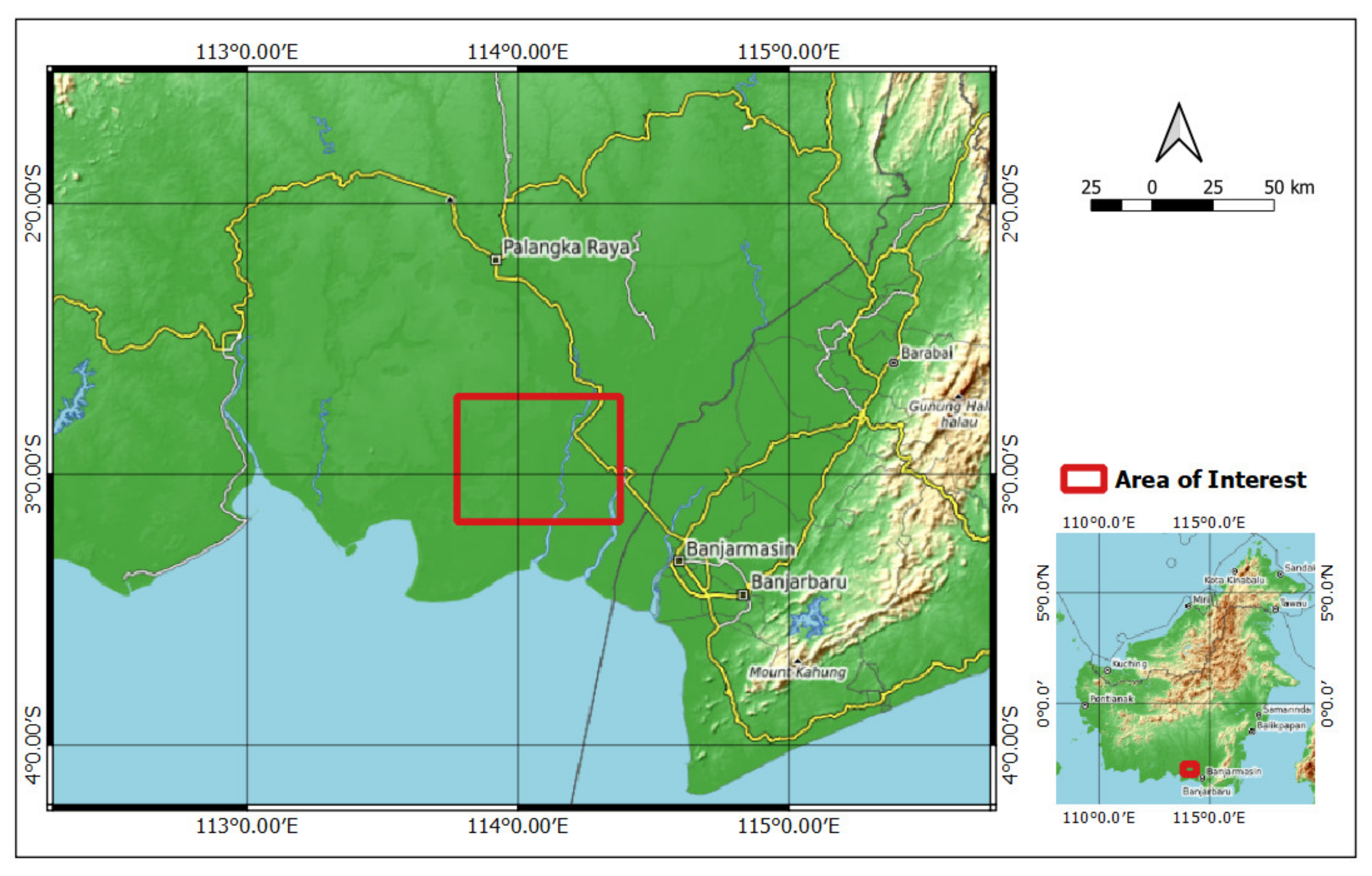
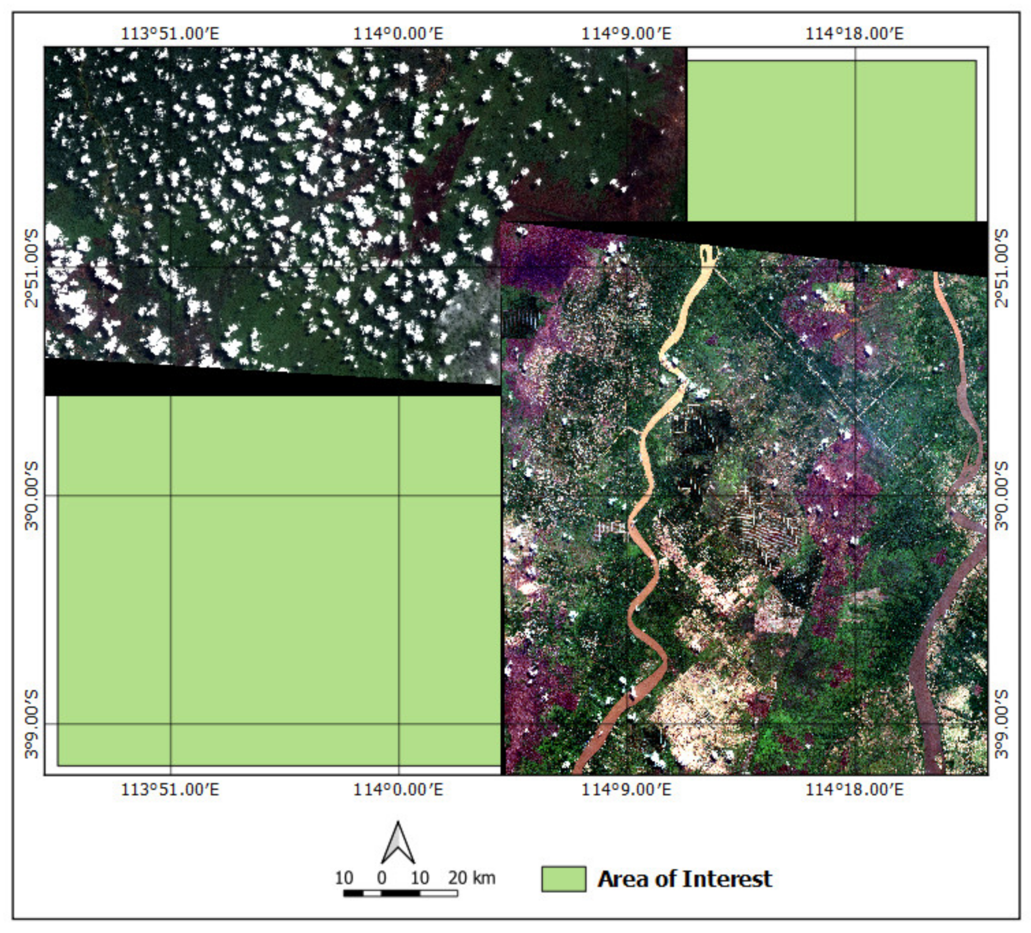
2.1. Research Area and Data

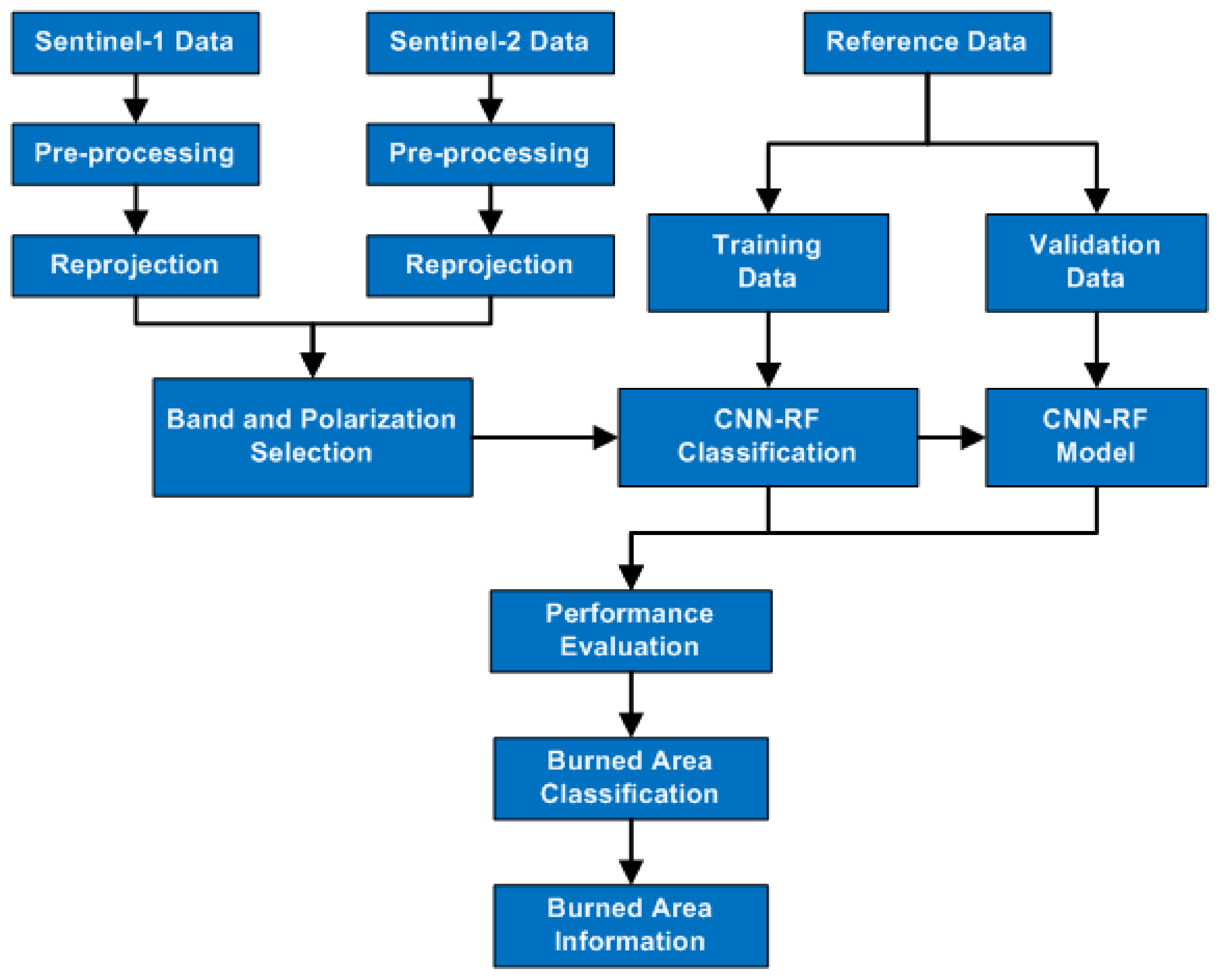
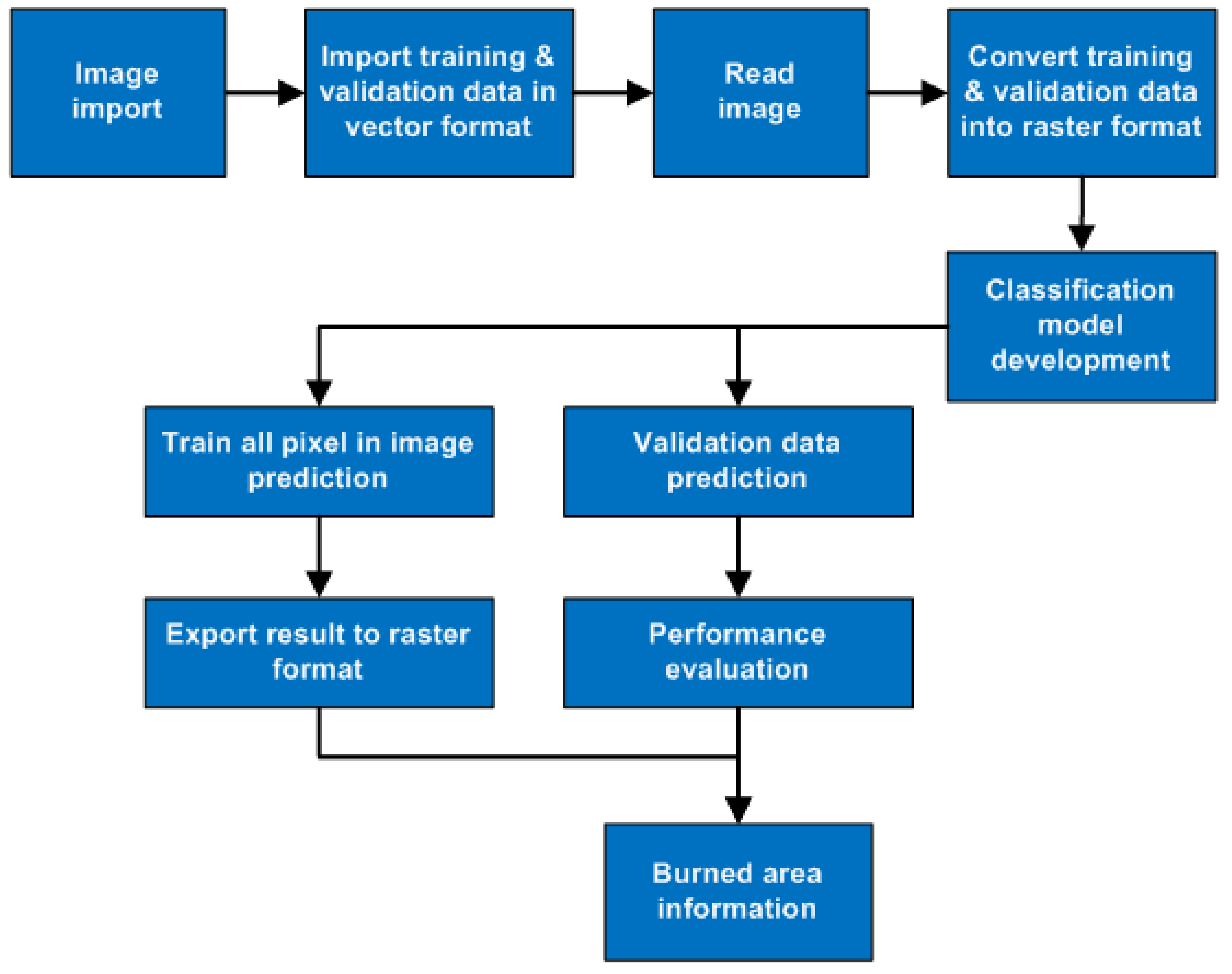
A part of the region of Pulang Pisau Regency and Kapuas Regency, Central Kalimantan, Indonesia (Figure 1), was selected as the research area as it has been one of the most affected regions in the last three years [4]. The land cover in this area comprises plantations, shrub swamps, and crops [39]. The size of the research area is approximately 344,600 hectares.

Sentinel-1 and Sentinel-2 data were selected in this research using Google Earth Engine. The multi-temporal data were used to avoid pixel gaps in the cloud cover area. In selecting the data, the percentage of cloud cover was considered since it influences the data quality; therefore, the optical remote sensing data used in this research has a cloud cover percentage of less than 20%.

Table 1. Specifications of Sentinel-1 and Sentinel-2 data used in the research [41,42].

Sensor	Specifications
Sentinel-2 MSI	Date	Pre-fire: July 2019		Post-fire: October 2019
	Bands	Band number	Band name	Resolution
		B2	Blue	10
		B3	Green	10
		B4	Red	10
		B5	Vegetation red edge 1	20
		B6	Vegetation red edge 2	20
		B7	Vegetation red edge 3	20
		B8	NIR	10
		B8A	Narrow NIR	20
		B11	SWIR1	20
		B12	SWIR2	20
	Product Level	L-2A
Sentinel-1 (C-Band SAR)	Date	Pre-fire: July 2019		Post-fire: October 2019
	Frequency	5.405 GHz
	Orbit	Descending
	Product Type	Ground range detected
	Acquisition Mode	Interferometric wide swath
	Polarization Mode	VV and VH

shows Sentinel-1 and Sentinel-2 data specifications used in this research. For pre-fire and post-fire events, we mosaicked cloudless Sentinel-2 data on 5–30 July 2019, and 8–23 October 2019, respectively. Mosaic SAR images of pre-fire events were taken on 6–23 July 2019, and 10–27 October 2019, for post-fire events from Sentinel-1 data. Figure 2 shows mosaic images of SAR and optical remote sensing data that were used in this research. The RGB SAR images are composed of VV polarization in pre-fire events and VH polarization in post-fire events, while RGB optical images are composed of B4, B3, and B2 in post-fire events.

In addition to using SAR and optical remote sensing data for conducting classification, as a reference, we used the 1.5 m resolution pan-sharpened Satellite pour de l’Observation de la Terre (SPOT) images dated 2 September and 8 October 2019. The Indonesian Geospatial Map, with a scale of 1:50,000 from the Geospatial Information Agency, was used to identify the land cover type in the research site [38]. The hotspot data trend from MODIS and Visible Infrared Imaging Radiometer Suite (VIIRS) sensor, acquired from the National Aeronautics and Space Administration (NASA), was used to support the existence of burned areas [40]. Moreover, MODIS burned area monthly global 500 m, MCD64A1, obtained from Google Earth Engine, was used in this research. The burned area from the Ministry of Environment and Forestry was used to determine the fire’s location and time.

2.2. Methodology

The proposed methodology of this research is described in Figure 3. It consists of several main sections, including image pre-processing, band and polarization selection, training and validation data production, classification, model evaluation, and burned area calculation.

Image pre-processing for SAR data produced gamma naught (γ⁰) and applied speckle filtering using a 5 × 5 Boxcar filter to improve image classification. In SAR data, this research used two backscatter coefficients: sigma naught (${\sigma }^0$) and gamma naught (γ⁰). ${\sigma }^0$ is the radar signals reflected per unit area in the ground range, whereas γ⁰ is radar reflectivity per unit area perpendicular to the slant range direction [43,44]. For optical data, pre-processing steps included cloud masking and resampling into 10 meters using bilinear interpolation. The function used for cloud masking was acquired from Principe [45]. In addition, reprojection was conducted in both sets of data, and all pre-processing steps were performed using Google Earth Engine. Figure 4 shows the area of interest that overlays with SPOT images on 2 September and 8 October 2019, as the reference data.

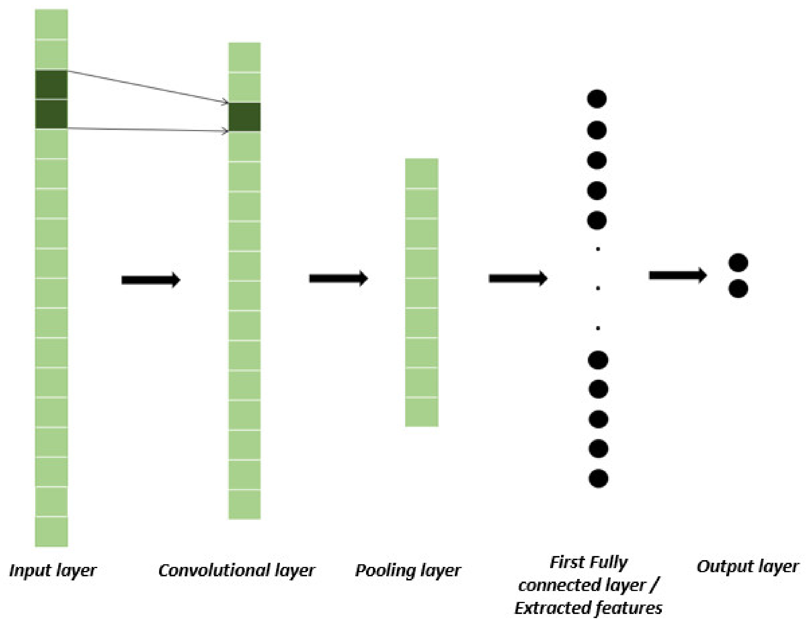
2.3. Convolutional Neural Network (CNN)

CNN is an artificial neural network that uses the convolution principle in data processing. It is a type of deep neural network that uses additional layers between the input and output layers [46]. The basic concept of CNN is to utilize a convolutional layer to detect the relationship between the features of objects and a pooling layer to group similar features. CNN architecture consists of at least one convolutional layer (CL), which transforms a set of activation functions with a differential function, each with a corresponding pooling layer (PL), and the final result is a fully connected layer (FCL) [29]. The pooling layer is used to reduce the size of an image by downsampling it and summarizing the features. The common pooling methods to achieve grouping are average pooling, where the summary is the dominant feature, and maximum pooling, by summarizing the strongest feature [47]. Unlike other neural networks where all neurons are fully connected with every other neuron of the next layer to recognize a pattern, CNN omits zero-valued parameters and makes fewer connections between layers. Non-zero parameters can be shared to be used by more than one connection in the layer to reduce the number of connections. CNN is a potent method, as structures of different dimensions can be constructed to adapt to input data of different dimensions, which can greatly affect final classification/prediction results. In addition, the representation of raw data is crucial because CNN is based on the principle of locality [48]. The basic CNN shown in Figure 5 uses a 1-dimensional array of data as the input layer, each pixel vector from different images represents the input data. The CL then downsamples the data, collects it by the PL, and it results in the FCL.

2.4. Random Forest (RF)

Random forest is an ensemble method modified from bootstrap aggregating, or bagging, developed from multiple uncorrelated trees. Bagging method generated a training dataset by randomly drawing replacement examples from the same number of the original training set of selected feature combinations [24]. Each tree in the bagging method is not fully independent since all predictor variables are taken into account on each splitting in a tree; therefore, the tree from different samples can have a similar structure called tree correlation. Random forest improves the bagging method by reducing the correlation and variance.

Samples are classified from the most popular (high vote) class from the decision tree predictors in the forest. Since the decision tree design requires attribute selection and pruning to optimize the choices, a tree was grown to its maximum depth every time by using new training data from a combination of features. As the number of trees increases, the generalization error converges with pruning. The number of features used at each node to generate a tree and the number of trees to be grown are user-defined parameters for the RF classifier [24].

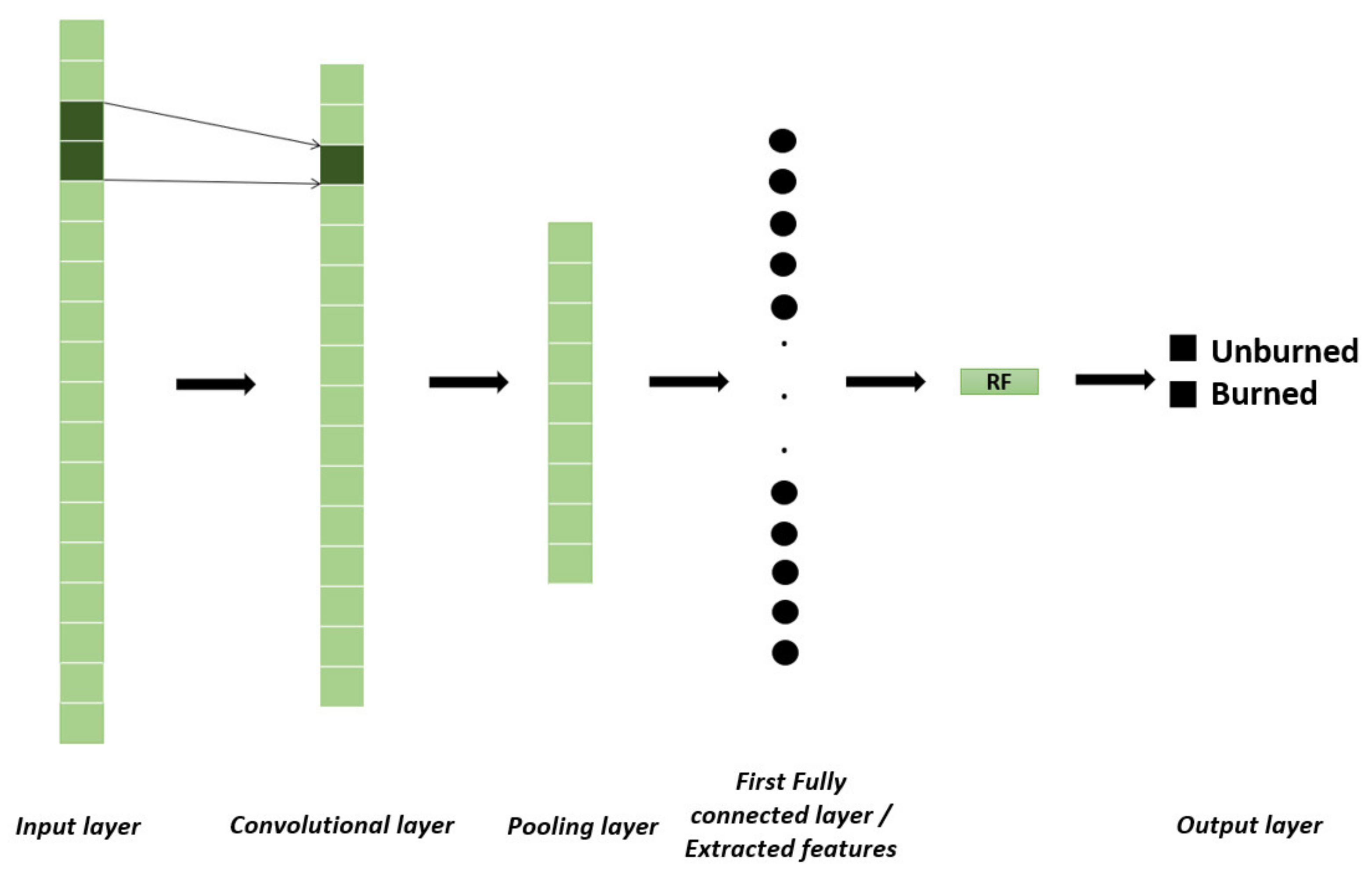
2.5. Proposed Method

The combined CNN and RF (CNN-RF) architecture is shown in Figure 6, which consists of an input layer derived from the image bands, a convolutional layer, a pooling layer, and a fully connected layer. The output of the first fully connected layer is the result of features extracted and then used as input for the classification of the burned area using the RF method.

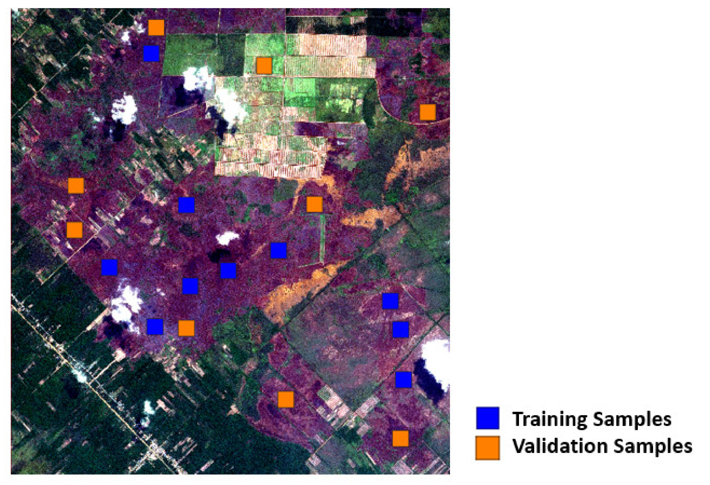
2.6. Training and Validation Dataset

The dataset was split into training and validation data that consisted of burned and unburned areas. As a reference to label burned and unburned samples in the training and validation dataset, this study used a high-resolution SPOT image, as seen in Figure 7, to minimize mixing pixels. It is a pan-sharpened image with a resolution of 1.5 meters. The training and validation were in polygon and classified at the pixel level. The dataset was designed to be balanced to decrease the effect of an imbalanced dataset. The comparison between training and validation samples was set to 70:30. Therefore, there were 176,100 pixels consisting of 88,460 pixels of burned and 87,640 of unburned classes for training, and 76,032 pixels consisting of 38,632 of burned and 37,400 of unburned classes for validation. Figure 7 shows the training and validation samples in the specific area of interest.

2.7. Classifiers Implementation

The model classification was performed using the Python programming language. Deep learning classifiers were conducted using “TensorFlow” and “Keras” libraries, while the RF classifier and performance evaluation were performed using the “Scikit-learn” library. Geospatial Data Abstraction Library (GDAL) was used in handling geospatial imagery, such as importing in raster format, importing vector data, reading the images, and converting data. The classification system of this research is shown in Figure 8.

The fixed hyperparameters for the CNN-RF classification method were the learning rate of 0.001, the epoch of 50, the batch size of 32, the dropout of 0.1, and the number of trees of 500. The CNN architecture was constructed of four layers that consisted of two convolutional layers, one pooling layer, and a fully connected layer. Kernel size was set at 2 × 2 with 24 filters on the convolutional layer. Stride was set to 1 to avoid downsampling, and padding was set to 0 to maintain the dimensions of the feature map generated from the input image. In each convolutional layer, we used rectified linear unit (ReLU). In the pooling layer, max pooling was used, taking the maximum value from the filter.

Meanwhile, the number of nodes for all schemes in the fully connected layer was set to 20. The sigmoid function was used in the output layer to meet the binary classification requirement. The loss function binary cross-entropy and Adam optimizer were used for the learning. The setting in these parameters was performed empirically as the optimal one. Classification models of burned areas were also carried out using the RF and CNN methods separately and the neural network (NN). The hyperparameters used in the CNN method are the same as those in the CNN-RF method. Meanwhile, the NN architecture consists of one input layer, two hidden layers, and one output layer.

2.8. Classification Scheme

Table 2. Input bands and polarizations for each classification scheme.

Scheme	Sensor	Band/Polarization
#1	Optical	20 bands of pre-fire and post-fire events
# 2	SAR	8 bands VV and VH polarization of ${\sigma }^0$ and ${\gamma }^0$ of pre-fire and post-fire events
# 3	Optical and SAR VH Polarization	optical band and VH polarization of ${\sigma }^0$ and ${\gamma }^0$ of pre-fire and post-fire events, with a total of 24 bands
# 4	Optical and SAR VV Polarization	optical band and VV polarization of ${\sigma }^0$ and ${\gamma }^0$ of pre-fire and post-fire events, with a total of 24 bands
# 5	Optical and SAR VH and VV Polarization	optical band and VH and VV polarization of ${\sigma }^0$ and ${\gamma }^0$ of pre-fire and post-fire events, with a total of 28 bands

lists the classification scheme used in this research as a classification input. The schemes were intended to evaluate the use of Sentinel-1 and Sentinel-2 data for burned area classification. Scheme #1 uses Sentinel-2 optical data with 20 bands; Scheme #2 uses Sentinel-1 SAR data with co-polarization (VV), cross-polarization (VH), and full-polarization (VH and VV). Schemes #3–#5 combine Scheme #1 and each polarization of Scheme #2. This study uses 10 bands of pre-fire (July) and 10 bands of post-fire (October) mosaicked images, resulting in 20 bands in Scheme #1. We mosaicked ${\sigma }^0$ and ${\gamma }^0$ SAR images in July and October, resulting in 8 bands in Scheme #2, 24 combined bands in Scheme #3–#4, and 28 combined bands in Scheme #5.

2.9. Evaluation Parameter

To evaluate the model, we used several parameters, such as overall accuracy (OA), precision, recall, F1-Score, and Cohen’s Kappa (K), as expressed in Equations (1)–(5). OA is the number of pixels that are classified correctly from the total number of pixels involving true positive (TP), true negative (TN), false positive (FP), and false negative (FN). Precision represents how many pixels are detected as a burned area out of the total predicted pixels. The recall represents how many of the burned areas can be detected correctly. F1-Score is the average precision and recall given a weight (harmonic mean). Cohen’s Kappa measures the level of agreement between the predicted results and the reference data in classifying pixels into specific classes. Cohen’s Kappa value ranges from −1 to 1. The p_e value in Equation (5) is the percentage change in measurement between the predicted results and the reference data.

$$\mathrm{Overall} \mathrm{Accuracy}=\frac{TP+TN}{TP+TN+FP+FN}$$

(1)

$$\mathrm{Precision}=\frac{TP}{TP+FP}$$

(2)

$$\mathrm{Recall}=\frac{TP}{TP+FN}$$

(3)

$$\mathrm{F}1-\mathrm{Score}=2\times \frac{\left(Precision\times Recall\right)}{\left(Precision+Recall\right)}$$

(4)

$$\mathrm{Cohen}’\mathrm{s} \mathrm{Kappa}=\frac{Overall accuracy-p_e}{1-p_e}$$

(5)

3. Results

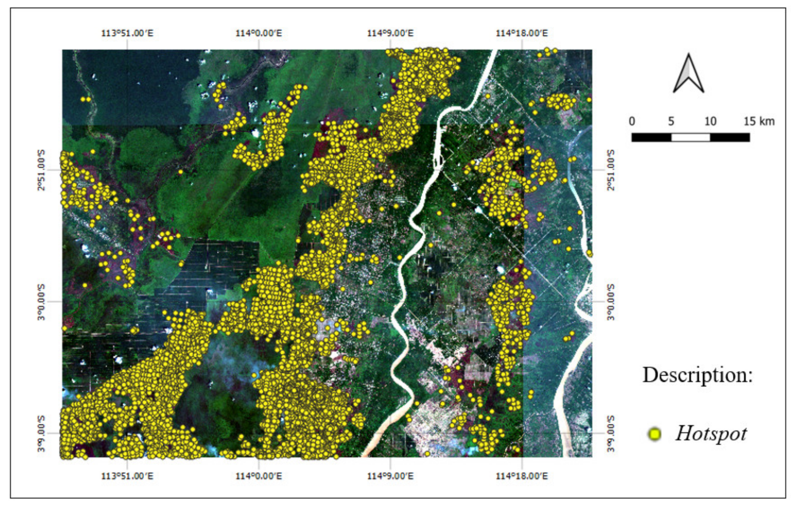
3.1. Hotspot Distribution Pattern

Based on MODIS and VIIRS sensors, the number of hotspots in the research site throughout 2019 with a medium to high confidence level is 14,030 spots, as shown in Figure 9, with the peak of fire incidence in September 2019, with as many as 9,740 spots. On the basis of the spatial resolution of the MODIS sensor for each hotspot pixel, the MODIS MCD64A1 correlates with the maximum extent of the burned area of 53,836 hectares. The results of the hotspot distribution pattern at the research location are shown in Figure 10. The distribution results can be used as supporting data to determine the time and location of the burned area.

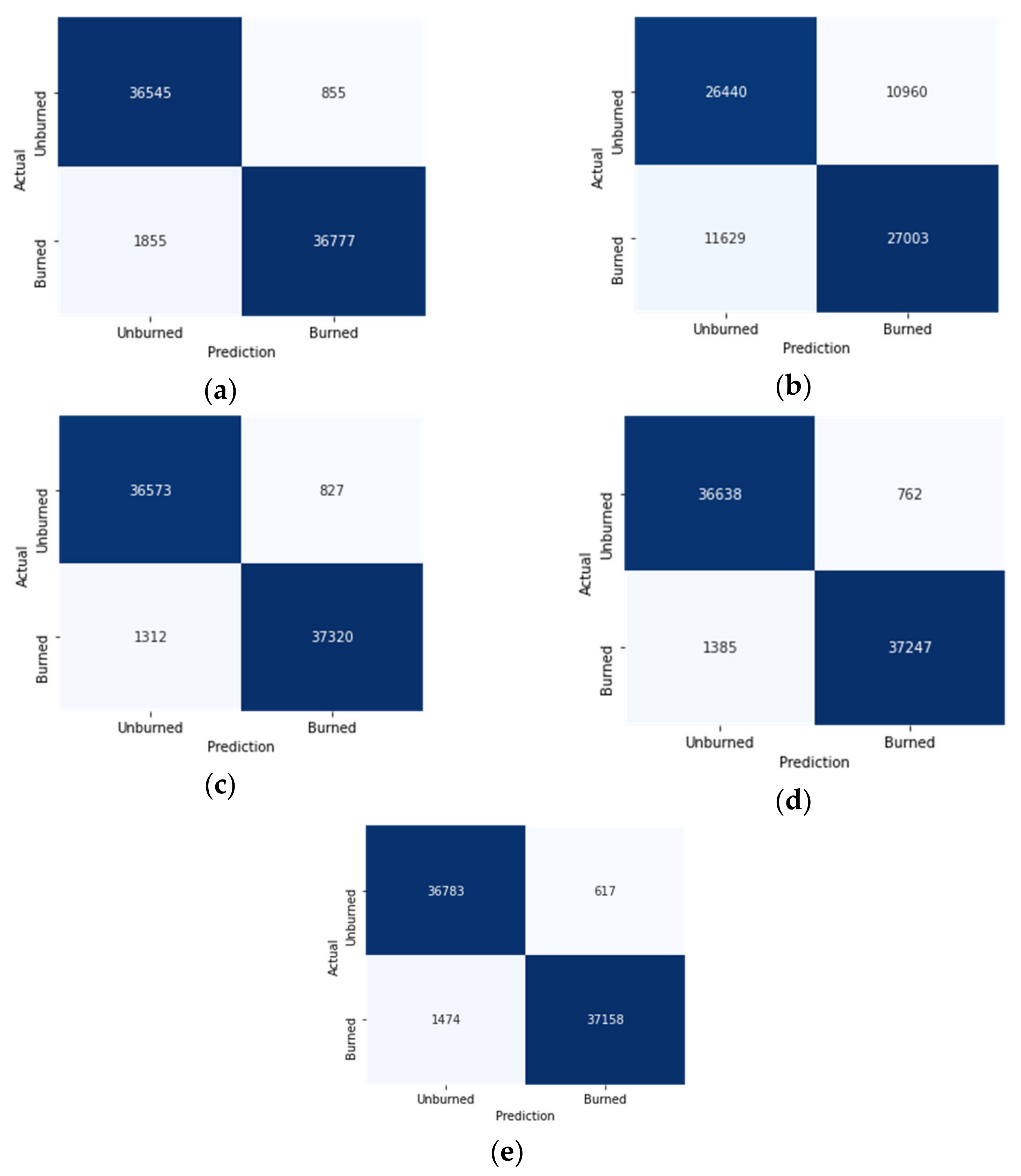
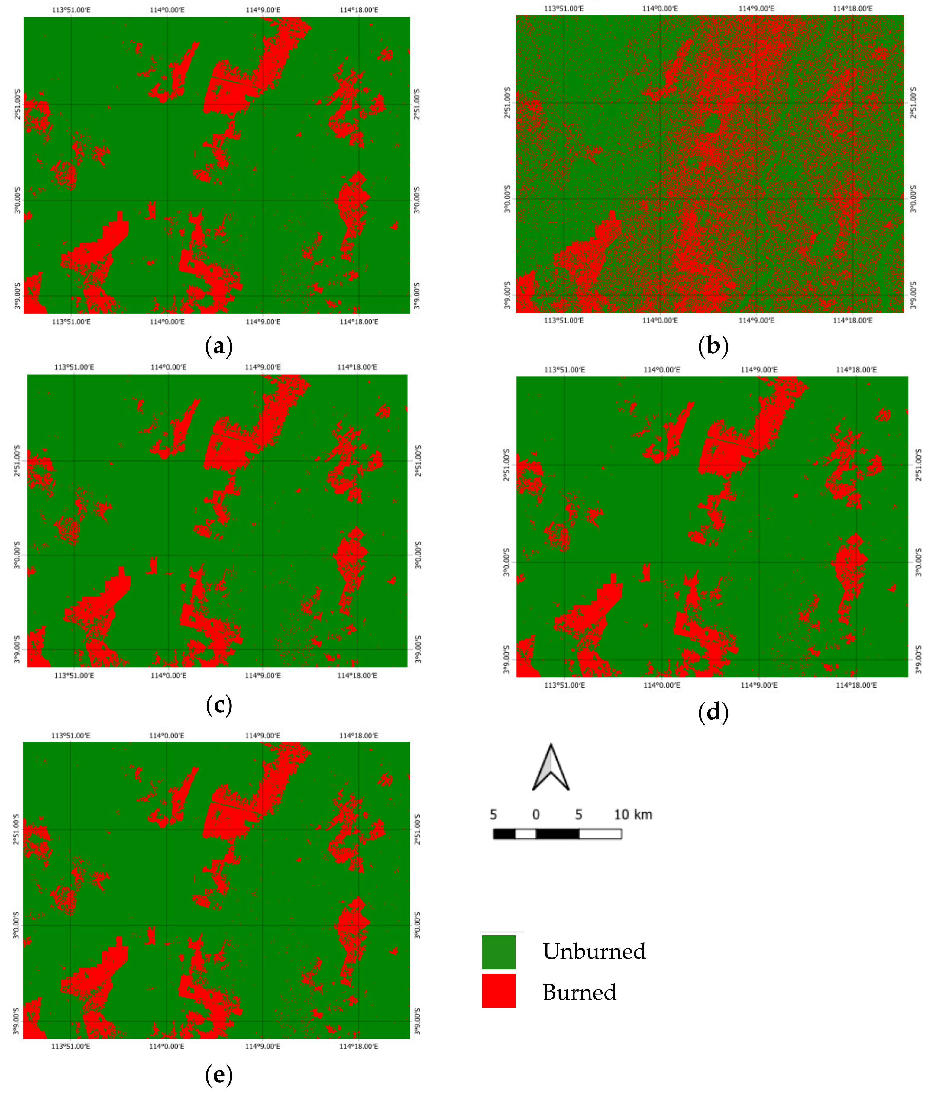
3.2. Classification Result of Burned Area using CNN-RF Method

Figure 11 shows the performance of the burned area classification model using the CNN-RF method for Schemes #1–#5, with parameters of OA, recall, precision, F1-score, and K-score. Overall accuracy is the probability that an individual data can be correctly classified, either true positive (i.e., correctly identified as burned area) or true negative (i.e., correctly removed as unburned area). The sum is divided by the total number of tests. Recall represents the CNN-RF’s ability to correctly identify the burned area from the actual data, while precision is the ability to detect burned areas from several tests. F1-score is the harmonic mean of precision and recall. K-score measured the performance of the CNN-RF on the basis of the agreement between the model and the actual data.

In Scheme #1, which is a classification involving only optical remote sensing data, the OA value was 0.9644. In addition, it obtained the recall and precision values at 0.9520 and 0.9773, respectively, indicating that over 95% of validation data can be predicted correctly. Meanwhile, the F1-score value was obtained at 0.9645 and K at 0.9282, indicating a strong agreement between prediction results and validation data. In Scheme #2, classification involving only SAR data provided the OA, recall, precision, F1-score, and K values of 0.7029, 0.6990, 0.7113, 0.7051, and 0.4058, respectively. Meanwhile, for Schemes #3–#5, the combination schemes between optical and SAR data involving VH, VV, and both polarizations, the OA values were 0.9719, 0.9718, and 0.9725, respectively. The recall values obtained were 0.9660, 0.9641, and 0.9618; the precision values were 0.9783, 0.9800, and 0.9837; the F1-scores were 0.9721, 0.9720, and 0.9726; and K values were 0.9437, 0.9435, and 0.9450, respectively.

On the basis of these results, it is shown that Scheme #5, which is a classification involving optical remote sensing data and SAR on VH as well as VV polarizations, provides the best model performance based on the parameters of OA, precision, F1-score, and K. Meanwhile, Scheme #3 obtained the best recall value compared with other schemes. The improvement of the model’s OA in Scheme #5 reached 0.81% compared with Scheme #1 and 26.96% compared with Scheme #2.

4. Discussion

Figure 12a–e shows the confusion matrix for Schemes #1–#5 using the CNN-RF method, which shows how the 76,032 pixels of the validation data were classified. In Scheme #2, the classification involving only SAR data resulted in the lowest performance. It misclassified 10,960 pixels as burned area and 11,629 pixels as unburned area. However, 70% of the pixels in Scheme #2 were classified correctly. In Scheme #5, where the classification involved optical remote sensing data and SAR on VH and VV polarization, it obtained the most minor false positive compared with other schemes: 617 pixels.

Meanwhile, the slightest false negative was achieved in Scheme #3. Based on the confusion matrix results, the number of false negatives was always greater than false positives in the entire scheme. Therefore, the resulting model shows that an unburned area was still incorrectly classified as burned.

The model in Schemes #1–#5 was then applied to classify the research site. These results for each scheme are shown in Figure 11a–e. In Scheme #2, SAR remote sensing data classified burned areas for the large-scale area (>300 hectares). The pattern of the burned area is shown in Figure 11b so that it can be used as supporting data for mapping burned areas. However, there were still high commission and omission errors that need to be improved. In addition, this integration method should be tested in other land cover types outside of this research’s area of interest since burned area product from SAR data is influenced by land cover types such as grassland [49].

In Figure 13, one can see that the most significant classification error was in Scheme #2. The reason is that the speckle filtering was not able to extract surface roughness information between objects, wherein some training data from the unburned class is shrub swamp, where 18% of the area in South Kalimantan is a peatland and waterlogged [50]. In addition, the presence of an open land area produced low-intensity backscatter coefficient values in VH and VV polarization. Meanwhile, the backscatter coefficient value trend of the burned area was low [21] due to the scattering mechanism that applies to the VH and VV polarization. Therefore, backscatter coefficient values can be similar between the burned and unburned areas. It can be concluded that using SAR remote sensing data without involving any features, such as texture feature or radar-based parameter, as the only input through pixel-based pre-processing is not effective enough using the CNN-RF method. In addition, to reduce commission error in Scheme #2, it is important to use additional data, such as hotspots, to discriminate between burned and unburned areas with a similar trend of backscatter coefficient values [49].

4.1. Comparison among CNN-RF, CNN, RF, and NN Methods

Table 3. The results of the performance of the burned area classification model using the CNN, RF, and NN methods, as well as the CNN-RF method for Schemes #1–#5.

Sensor	Scheme	CNN
		OA	Recall	Precision	F1 -Score	K
Optical	#1	0.9619	0.9475	0.9767	0.9619	0.9237
SAR	#2	0.7136	0.7553	0.7030	0.7282	0.4263
Optical and SAR	#3	0.9676	0.9665	0.9697	0.9681	0.9352
	#4	0.9716	0.9793	0.9653	0.9723	0.9432
	#5	0.9682	0.9519	0.9849	0.9681	0.9363
		RF
Optical	#1	0.9580	0.9427	0.9738	0.9580	0.9160
SAR	#2	0.6991	0.6908	0.7094	0.7000	0.3983
Optical and SAR	#3	0.9621	0.9498	0.9749	0.9622	0.9241
	#4	0.9635	0.9513	0.9763	0.9636	0.9271
	#5	0.9636	0.9525	0.9753	0.9638	0.9272
		NN
Optical	#1	0.9611	0.9602	0.9632	0.9617	0.9223
SAR	#2	0.6953	0.6614	0.7170	0.6881	0.3912
Optical and SAR	#3	0.9548	0.9742	0.9391	0.9563	0.9095
	#4	0.9506	0.9483	0.9543	0.9512	0.9012
	#5	0.9580	0.9593	0.9580	0.9587	0.9159
		CNN-RF
Optical	#1	0.9644	0.9520	0.9773	0.9645	0.9287
SAR	#2	0.7029	0.6990	0.7113	0.7051	0.4058
Optical and SAR	#3	0.9719	0.9660	0.9783	0.9721	0.9437
	#4	0.9718	0.9641	0.9800	0.9720	0.9435
	#5	0.9725	0.9618	0.9837	0.9726	0.9450

shows the performance comparison of the burned area classification model for Schemes #1–#5, with parameters such as OA, recall, precision, F1-score, and K. Based on Table 3, the highest OA and K values were found in the CNN-RF method in the tested schemes, except in Scheme #2. The highest values are printed in bold.

Based on the recall parameter, the NN method has the highest recall values in Scheme #1 to Scheme #3. Meanwhile, the CNN method has the highest recall values for Schemes #2 and #4. Furthermore, the highest recall value for Scheme #5 was achieved using the CNN-RF method. For the precision parameter, the highest precision value resulted from the CNN-RF method for Schemes #1, #3, and #4, while the highest precision values for Schemes #2 and #5 were found in the NN and CNN methods, respectively, as shown in Table 3. Table 3 also shows that the trend of the precision value was always higher than the recall for the CNN-RF method. An accurate burned area estimation is important [20], and improved burned area estimation can be achieved by identifying and minimizing false positives [51]. The CNN-RF method’s results increased the precision value in the obtained model classification. Hence, this method is promising in improving burned area estimation.

In the case of F1-score parameter, the highest value was retrieved using the CNN-RF method for Schemes #1, #3, and #5, among other methods. In addition, the CNN method had the highest F1-score for Schemes #2 and #4. For the K parameter, the highest value resulted from the CNN-RF method, except for Scheme #2.

This research also showed that using SAR remote sensing data in Scheme #2 for the four methods provides the lowest performance compared with other schemes. For this scheme, OA values of 0.7136, 0.6991, 0.6953, and 0.7029 resulted from CNN, RF, NN, and CNN-RF, respectively. The highest accuracy, recall, F1-Score, and K values were achieved using the CNN method for Scheme #2. Meanwhile, the NN method had the highest precision value. Although the overall accuracy was low compared with other schemes, the current use of machine learning classification methods for SAR data was in the range of 0.70–0.75 [29,47,48]. The obtained K value was also the lowest because the agreement score range was approximately 0.4.

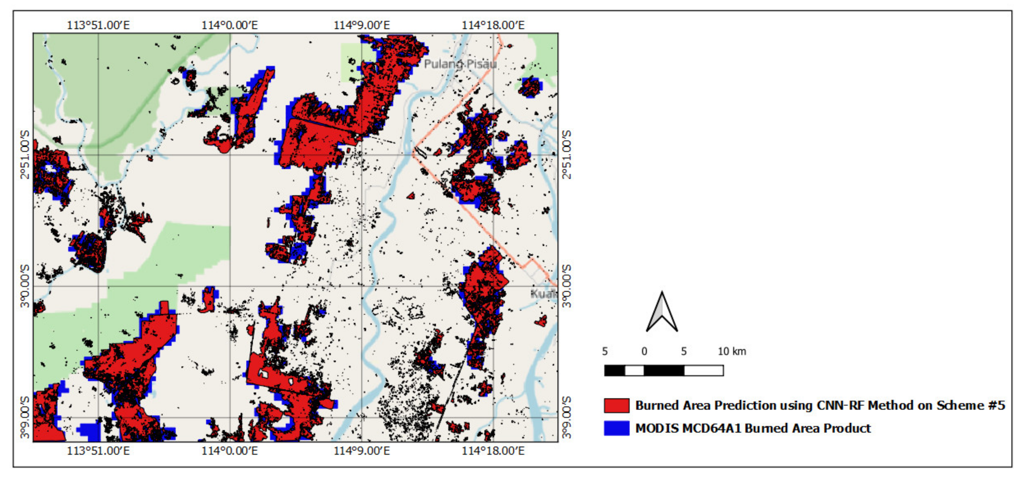
4.2. Burned Area Estimation

The burned area was calculated using the CNN, RF, NN, and CNN-RF methods using WGS 1984 PDC Mercator as a reference projection system.

Table 4. Burned area estimation using CNN, RF, NN, and CNN-RF methods.

Scheme	Burned Area Estimation (Hectares)
	CNN	RF	NN	CNN-RF
#1	47,834.74	47,762.48	51,749.67	48,367.02
#2	112,691.83	108,029.40	96,339.55	106,945.36
#3	51,750.16	47,536.03	55,671.40	48,735.11
#4	50,428.16	47,659.81	51,366.37	48,514.23
#5	47,903.56	47,433.93	50,783.50	48,824.59

shows the prediction results of burned area for each scheme, where for the CNN-RF method, the area obtained was 48,367.02 hectares for Scheme #1, 106,945.36 hectares for Scheme #2, 48,735.11 hectares for Scheme #3, 48,514.23 hectares for Scheme #4, and 48,824.59 hectares for Scheme #5. The largest area result was obtained in Scheme #2, which involved only SAR remote sensing data, and the results were obtained from a model with low precision and K values so that the largest chance of error in the estimation was in this scheme.

As burned area information from the field survey is in the form of coordinate points, MODIS MCD64A1 burned area product was used as a comparison. Figure 14 compares burned area result prediction using the CNN-RF method on Scheme #5 and MODIS MCD64A1 burned area product. Using the same reference projection system, burned area estimation from MODIS in the area of interest was 53,836.08 hectares. It shows that the obtained burned area estimation using the CNN-RF method had 89–90% agreement with MCD64A1 burned area product for Schemes #1, #3–#5. However, the burned area estimation using SAR remote sensing data for all tested methods in Scheme #2 tended to be larger than optical remote sensing data or combined optical and SAR data. The burned area proportion from the MODIS MCD64A1 products was 47–55% of those obtained from this research.

5. Conclusions

It can be concluded that optical-based classification, SAR-based classification, and combined optical and SAR data classification are reliable methods for burned area identification using a hybrid CNN-RF method. The CNN-RF method on the combined optical remote sensing and full-polarization SAR data can be used as the best method to identify the burned area, with the highest overall accuracy reaching 97.25%, with the burned area being 48,824.59 hectares, yielding 90% accuracy compared with MCD64A1 burned area product data. Estimation results using only SAR data with the CNN-RF method can be used only as supporting data for identifying the burned area. For further research, using physical parameters of radar or grey level co-occurrence matrix needs to be examined to improve classification performance using only SAR data.

In future works, to be applicable throughout Indonesia, this model needs to be tested using different datasets to increase model performance and maintain the stability of classification accuracy. In addition, it is crucial to investigate this model in different landscape characteristics, such as peatland in Sumatera and Kalimantan and savanna in East Nusa Tenggara Province. The object-oriented approach using high-resolution data also needs to be investigated for better results.

References

1. Government of the Republic of Indonesia. Presidential Regulation of the Republic of Indonesia Number 18/2020 Concerning the 2020–2024 National Mid-Term Development Plan; Republic of Indonesia: Jakarta, Indonesia, 2020. [Google Scholar]
2. Ministry of National Development and Planning. Metadata Indikator Tujuan Pembangunan Berkelanjutan (TPB)/Sustainable Development Goals (SDGs) Indonesia Pilar Pembangunan Lingkungan; The Ministry of National Development Planning Republic of Indonesia: Jakarta, Indonesia, 2020. [Google Scholar]
3. Enríquez-de-Salamanca, Á. Contribution to Climate Change of Forest Fires in Spain: Emissions and Loss of Sequestration. J. Sustain. For. 2019, 39, 417–431. [Google Scholar] [CrossRef]
4. Rekapitulasi Luas Kebakaran Hutan dan Lahan (Ha) Per Provinsi di Indonesia Tahun 2015–2020 (Data s/d 30 September 2020). Available online: https://sipongi.menlhk.go.id/hotspot/luas_kebakaran (accessed on 10 October 2021).
5. The World Bank. Indonesia Economic Quarterly: Investing People; The World Bank: Bretton Woods, NH, USA, 2019. [Google Scholar]
6. Marlier, M.E.; Liu, T.; Yu, K.; Buonocore, J.J.; Koplitz, S.N.; DeFries, R.S.; Mickley, L.J.; Jacob, D.J.; Schwartz, J.; Wardhana, B.S.; et al. Fires, smoke exposure, and public health: An integrative framework to maximize health benefits from peatland restoration. GeoHealth 2019, 3, 178–189. [Google Scholar] [CrossRef] [Green Version]
7. Harrison, M.E.; Page, S.E.; Limin, S.H. The global impact of Indonesian forest fires. Biologist 2009, 56, 156–163. [Google Scholar]
8. Roteta, E.; Bastarrika, A.; Padilla, M.; Storm, T.; Chuvieco, E. Development of a Sentinel-2 burned area algorithm: Generation of a small fire database for sub-saharan Africa. Remote Sens. Environ. 2019, 222, 1–17. [Google Scholar] [CrossRef]
9. Huang, H.; Roy, D.; Boschetti, L.; Zhang, H.; Yan, L.; Kumar, S.; Gomez-Dans, J.; Li, J. Separability analysis of Sentinel-2A multi-spectral instrument (MSI) data for burned area Discrimination. Remote Sens. 2016, 8, 873. [Google Scholar] [CrossRef] [Green Version]
10. Fornacca, D.; Ren, G.; Xiao, W. Evaluating the best spectral indices for the detection of burn scars at several post-fire dates in a Mountainous Region of Northwest Yunnan, China. Remote Sens. 2018, 10, 1196. [Google Scholar] [CrossRef] [Green Version]
11. Filipponi, F. BAIS2: Burned Area Index for Sentinel-2. Proceedings 2018, 2, 364. [Google Scholar]
12. Schowengerdt, R.A. Remote Sensing: Models and Methods for Image Processing, 3rd ed.; Elsevier: New Delhi, India, 2007. [Google Scholar]
13. Weng, Q. Principles of Remote Sensing. In Remote Sensing and GIS Integration Theories, Methods, and Applications: Theory, Methods, and Applications; McGraw-Hill: New York, NY, USA, 2010. [Google Scholar]
14. Lasaponara, R.; Tucci, B. Identification of Burned Areas and Severity Using SAR Sentinel-1. IEEE Geosci. Remote Sens. Lett. 2019, 16, 917–921. [Google Scholar] [CrossRef]
15. De Luca, G.; Modica, G.; Fattore, C.; Lasaponara, R. Unsupervised burned area mapping in a protected natural site. an approach using SAR Sentinel-1 data and K-mean algorithm. In Computational Science and Its Applications—ICCSA 2020; Springer Nature: Berlin/Heidelberg, Germany, 2020. [Google Scholar]
16. Lestari, A.I.; Rizkinia, M.; Sudiana, D. Evaluation of Combining Optical and SAR Imagery for Burned Area Mapping using Machine Learning. In Proceedings of the IEEE 11th Annual Computing and Communication Workshop and Conference (CCWC) 2021, Las Vegas, NV, USA, 27–30 January 2021; pp. 52–59. [Google Scholar]
17. Mutai, S.C. Analysis of Burnt Scar Using Optical and Radar Satellite Data. Master’s Thesis, University of Twente, Enschede, The Netherlands, 2019. [Google Scholar]
18. Ramo, R.; Chuvieco, E. Developing a random forest algorithm for MODIS global burned area classification. Remote Sens. 2017, 9, 1193. [Google Scholar] [CrossRef] [Green Version]
19. Ngadze, F.; Mpakairi, K.S.; Kavhu, B.; Ndaimani, H.; Maremba, M.S. Exploring the utility of Sentinel-2 MSI and Landsat 8 OLI in burned area mapping for a heterogenous savannah landscape. PLoS ONE 2020, 15, e0232962. [Google Scholar] [CrossRef]
20. Gaveau, D.L.A.; Descals, A.; Salim, M.A.; Sheil, D.; Sloan, S. Refined 1 burned-area mapping protocol using Sentinel-2 data 2 increases estimate of 2019 Indonesian burning. Earth Syst. Sci. Data 2021, 13, 5353–5368. [Google Scholar] [CrossRef]
21. Carreiras, J.M.B.; Quegan, S.; Tansey, K.; Page, S. Sentinel-1 observation frequency significantly increases burnt area detect-ability in tropical SE Asia. Environ. Res. Lett. 2020, 15, 54008. [Google Scholar] [CrossRef]
22. Widodo, J.; Riza, H.; Herlambang, A.; Arief, R.; Razi, P.; Kurniawan, F.; Izumi, Y.; Perissin, D.; Sumantyo, J.T.S. Forest Areas with a High Potential Risk of Fire Mapping on Peatlands Using Interferometric Synthetic Aperture Radar. In Proceedings of the 2021 7th Asia-Pacific Conference on Synthetic Aperture Radar (APSAR), Bali, Indonesia, 1–3 November 2021; pp. 1–4. [Google Scholar]
23. Corcoran, J.; Knight, J.; Gallant, A. Influence of multi-source and multitemporal remotely sensed and ancillary data on the accuracy of random forest classification of wetlands in northern Minnesota. Remote Sens. 2013, 5, 3212–3238. [Google Scholar] [CrossRef] [Green Version]
24. Pal, M. Random forest classifier for remote sensing classification. Int. J. Remote Sens. 2005, 26, 217–222. [Google Scholar] [CrossRef]
25. Al-Rawi, K.R.; Casanova, J.L.; Calle, A. Burned area mapping system and fire detection system, based on neural networks and NOAA-AVHRR imagery. Int. J. Remote Sen. 2001, 22, 2015–2032. [Google Scholar] [CrossRef]
26. Langford, Z.; Kumar, J.; Hoffman, F. Wildfire mapping in interior Alaska using deep neural networks on imbalanced datasets. In Proceedings of the IEEE International Conference on Data Mining Workshops (ICDMW), Singapore, 17–20 November 2018. [Google Scholar]
27. Hu, Y.; Zhang, Q.; Zhang, Y.; Yan, H. A deep convolution neural network method for land cover mapping: A case study of Qinhuangdao, China. Remote Sens. 2018, 10, 2053. [Google Scholar] [CrossRef] [Green Version]
28. Jozdani, S.E.; Johnson, B.A.; Chen, D. Comparing deep neural networks, ensemble classifiers, and support vector machine algorithms for object-based urban land use/land cover classification. Remote Sens. 2019, 11, 1713. [Google Scholar] [CrossRef] [Green Version]
29. Riyanto, I.; Rizkinia, M.; Arief, R.; Sudiana, D. Three-Dimensional Convolutional Neural Network on Multi-Temporal Synthetic Aperture Radar Images for Urban Flood Potential Mapping in Jakarta. Appl. Sci. 2022, 12, 1679. [Google Scholar] [CrossRef]
30. Kussul, N.; Lavreniuk, M.; Skakun, S.; Shelestov, A. Deep learning classification of land cover and crop types using remote sensing data. IEEE Geosci. Remote Sens. Lett. 2017, 14, 778–782. [Google Scholar] [CrossRef]
31. Wang, Y.; Li, Y.; Song, Y.; Rong, X. The Influence of the activation function in a convolution neural network model of facial expression recognition. Appl. Sci. 2020, 10, 1897. [Google Scholar] [CrossRef] [Green Version]
32. Ban, Y.; Zhang, P.; Nascetti, A.; Bevington, A.R.; Wulder, M.A. Near real-time wildfire progression monitoring with Sentinel-1 SAR time series and deep learning. Sci. Rep. 2020, 10, 1322. [Google Scholar] [CrossRef] [PubMed] [Green Version]
33. Stroppiana, D.; Azar, R.; Calò, F.; Pepe, A.; Imperatore, P.; Boschetti, M.; Silva, J.; Brivio, P.; Lanari, R. Integration of optical and SAR data for burned area mapping in mediterranean regions. Remote Sens. 2015, 7, 1320–1345. [Google Scholar] [CrossRef]
34. Guidici, D.; Clark, M. One-dimensional convolutional neural network land-cover classification of multi-seasonal hyper-spectral imagery in the San Francisco Bay Area, California. Remote Sens. 2017, 9, 629. [Google Scholar] [CrossRef] [Green Version]
35. Kiranyaz, S.; Avci, O.; Abdeljaber, O.; Ince, T.; Gabbouj, M.; Inman, D.J. 1D convolutional neural networks and applications: A survey. Mech. Syst. Signal Process. 2021, 151, 107398. [Google Scholar] [CrossRef]
36. Republic of Indonesia. Government Regulation Number 11 of 2018 Concerning Procedures for the Implementation of Remote Sensing Activities; Republic of Indonesia: Jakarta, Indonesia, 2018. [Google Scholar]
37. Song, Y.; Zhang, Z.; Baghbaderani, R.K.; Wang, F.; Qu, Y.; Stuttsy, C.; Qi, H. Land cover classification for satellite images through 1D CNN. In Proceedings of the 10th Workshop on Hyperspectral Imaging and Signal Processing: Evolution in Remote Sensing (WHISPERS), Amsterdam, The Netherlands, 24–26 September 2019; pp. 1–5. [Google Scholar]
38. Zhang, A.; Lipton, Z.C.; Li, M.; Smola, A.J. Dive into deep learning Release 0.16.6. arxiv 2021, arXiv:2106.11342v1. [Google Scholar]
39. Peta Rupa Bumi Indonesia. Available online: https://tanahair.indonesia.go.id/portal-web (accessed on 14 October 2021).
40. Fire Information for Resource Management System. Available online: https://firms.modaps.eosdis.nasa.gov/download/ (accessed on 3 July 2021).
41. Sentinel-2 Handbook. Available online: https://sentinel.esa.int/documents/247904/685211/Sentinel-2_User_Handbook (accessed on 13 August 2021).
42. Sentinel-1 ESA’s Radar Observatory Mission for GMES Operational Services. Available online: https://sentinel.esa.int/documents/247904/349449/S1_SP-1322_1.pdf (accessed on 13 August 2021).
43. Calculation of Beta Naught and Sigma Naught for TerraSAR-X Data. Available online: https://www.intelligence-airbusds.com/files/pmedia/public/r465_9_tsxx-airbusds-tn-0049-radiometric_calculations_d1.pdf (accessed on 3 March 2022).
44. Small, D.; Miranda, N.; Meier, E. A revised radiometric normalisation standard for SAR. In Proceedings of the IEEE International Geoscience & Remote Sensing Symposium (IGARSS), Cape Town, South Africa, 12–17 July 2009; pp. 566–569. [Google Scholar]
45. Cloud Mask. Available online: https://github.com/fitoprincipe/geetools-code-editor/blob/master/cloud_masks (accessed on 10 September 2021).
46. Belenguer-Plomer, M.A.; Tanase, M.A.; Fernandez-Carrillo, A.; Chuvieco, E. CNN-based burned area mapping using radar and optical data. Remote Sens. Environ. 2021, 260, 112468. [Google Scholar] [CrossRef]
47. Scherer, D.; Müller, A.; Behnke, S. Evaluation of Pooling Operations in Convolutional Architectures for Object Recognition. In Proceedings of the International Conference on Artificial Neural Networks (ICANN) 2010, Thessaloniki, Greece, 15–18 September 2010; pp. 92–101. [Google Scholar]
48. Wang, Y.; Fang, Z.; Hong, H.; Peng, L. Flood susceptibility mapping using convolutional neural network frameworks. J. Hydrol. 2020, 582, 124482. [Google Scholar] [CrossRef]
49. Belenguer-Plomer, M.A.; Tanase, M.A.; Fernandez-Carrilo, A.; Chuvienco, R. Burned area detection and mapping using Sentinel-1 backscatter coefficient and thermal anomalies. Remote Sens. Environ. 2019, 233, 111345. [Google Scholar] [CrossRef]
50. Taufik, M.; Veldhuizen, A.A.; Wösten, J.H.M.; van Lanen, H.A.J. Exploration of the importance of physical properties of In-donesian peatlands to assess critical groundwater table depths, associated drought and fire hazard. Geoderma 2019, 347, 160–169. [Google Scholar] [CrossRef]
51. Van Dijk, D.; Shoaie, S.; Van Leeuwen, T.; Veraverbeke, S. Spectral signature analysis of false positive burned area detection from agricultural harvests using Sentinel-2 data. Int. J. Appl. Earth Obs. Geoinf. 2021, 97, 102296. [Google Scholar] [CrossRef]
Figure 1. A part of the region of Pulang Pisau Regency and Kapuas Regency, Central Kalimantan, Indonesia as the area of interest.
Remotesensing 15 00728 g001
Figure 2. Mosaic Sentinel-1 SAR images (left) and Sentinel-2 optical images (right) used in the area of interest.
Remotesensing 15 00728 g002
Figure 3. Research workflow.
Remotesensing 15 00728 g003
Figure 4. A coverage of SPOT data as the reference within the area of interest in Figure 2.
Remotesensing 15 00728 g004
Figure 5. Illustration of 1-Dimension Convolutional Neural Network.
Remotesensing 15 00728 g005
Figure 6. The architecture of a hybrid of CNN and RF method (CNN-RF).
Remotesensing 15 00728 g006
Figure 7. Selected training and validation sample locations.
Remotesensing 15 00728 g007
Figure 8. Classification system.
Remotesensing 15 00728 g008
Figure 9. Hotspot intensity per month at the research site throughout 2019.
Remotesensing 15 00728 g009
Figure 10. The distribution of hotspots at the research sites throughout 2019.
Remotesensing 15 00728 g010
Figure 11. Performance of burned area classification model using CNN-RF method for Schemes #1–#5 with evaluation parameters (a) OA; (b) recalls; (c) precision; F1-score; and (d) Cohen’s Kappa.
Remotesensing 15 00728 g011
Figure 12. (ae) Confusion matrix classification of the burned area using CNN-RF method for Schemes #1–#5.
Remotesensing 15 00728 g012
Figure 13. The classification results using the CNN-RF method in the Schemes: (a) #1; (b) #2; (c) #3; (d) #4; and (e) #5.
Remotesensing 15 00728 g013
Figure 14. Comparison of burned area prediction using the CNN-RF method on Scheme #5 and MODIS MCD64A1 burned area product in the study area in July-October.
Remotesensing 15 00728 g014