

Assessment of L-Band SAOCOM InSAR Coherence and Its Comparison with C-Band: A Case Study over Managed Forests in Argentina


Abstract
1. Introduction
2. Materials and Methods
2.1. Interferometric SAR Principles
2.2. Interferometric Coherence
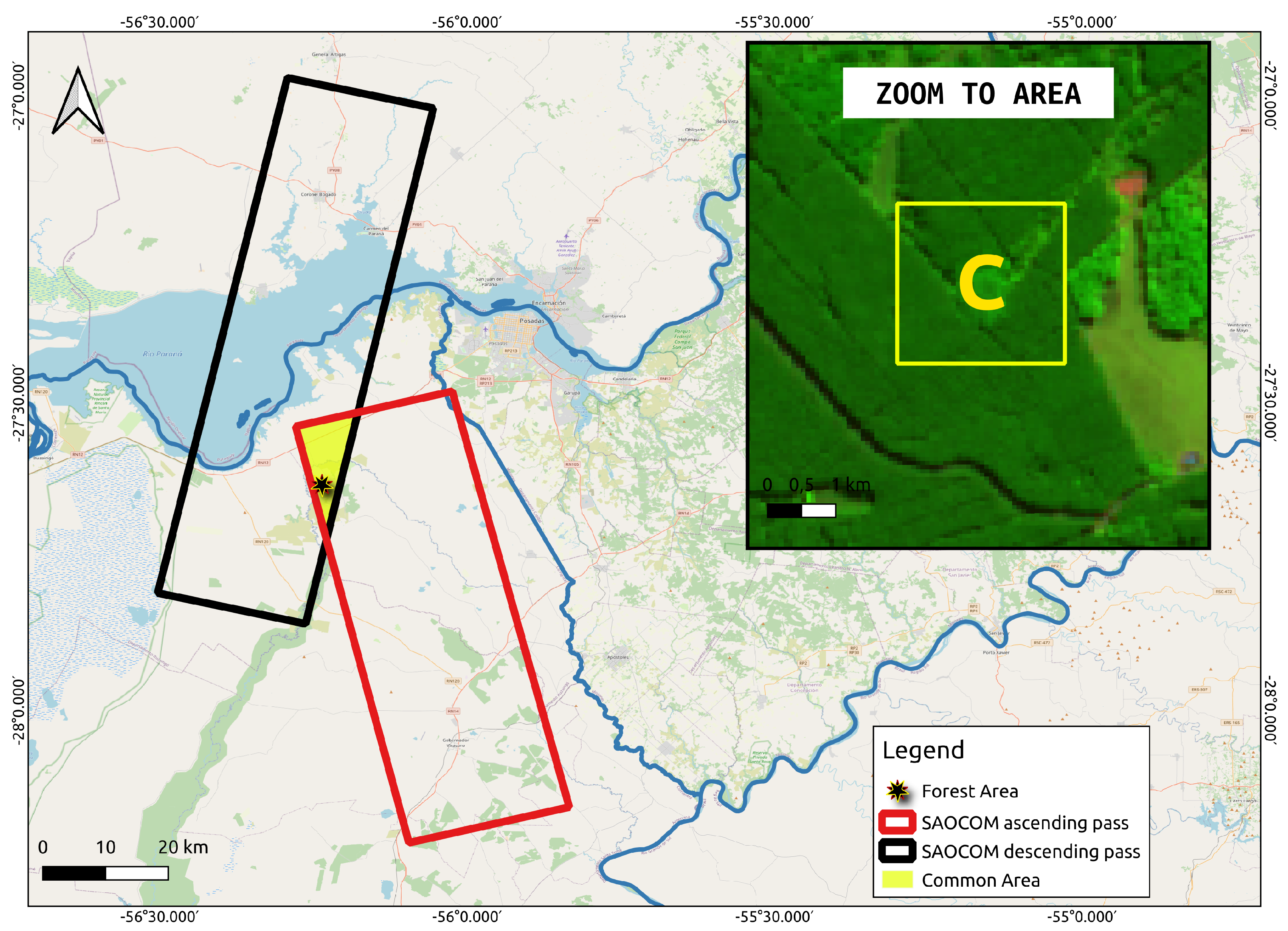
2.3. Study Areas
2.4. SAR Data
2.5. GEDI Data
3. Results
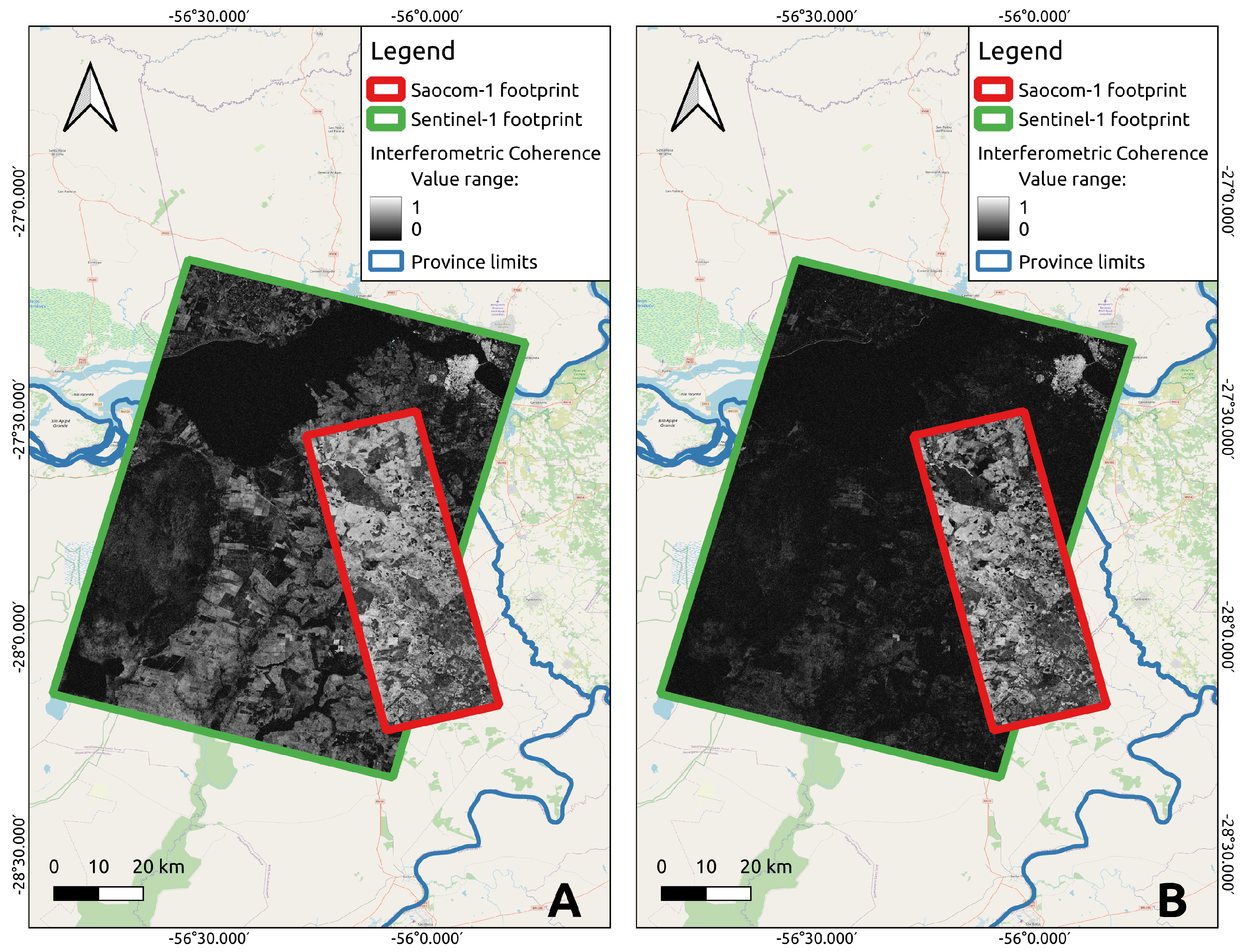
3.1. Coherence Maps
3.2. Ascending/Descending Orbits
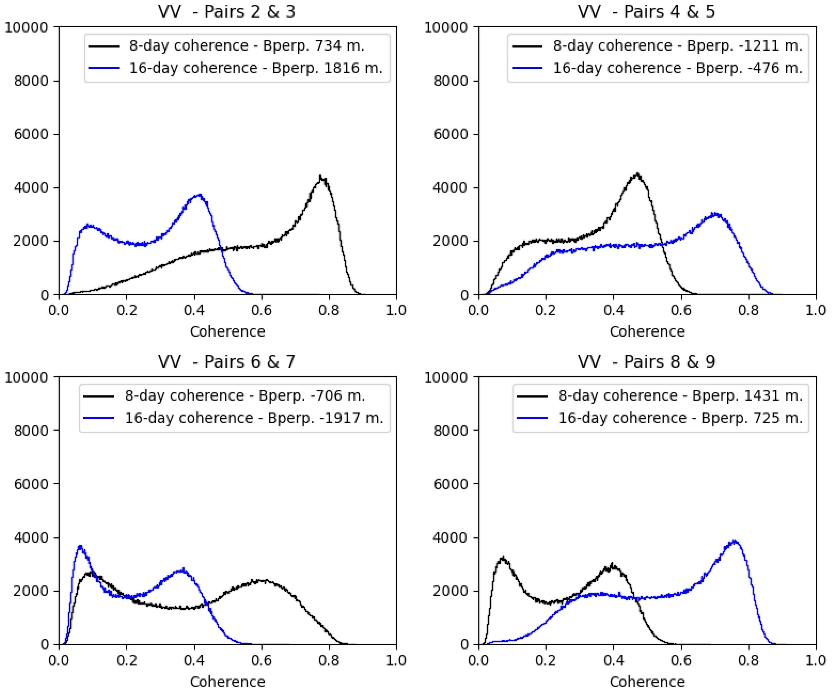
3.3. SAOCOM-1 8-Day Coherence
3.4. Forest Canopy Height
4. Discussion
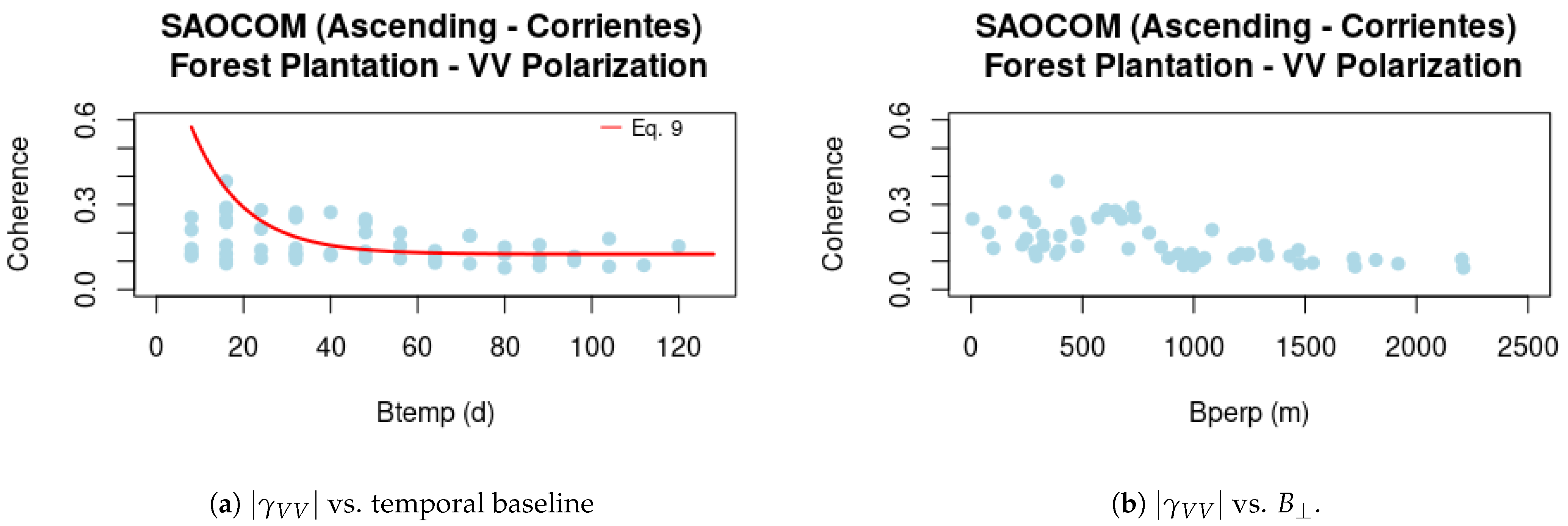
4.1. Spatial and Temporal Baselines
4.2. Polarimetry
4.3. Orbits Analysis
4.4. Short Temporal Baselines
4.5. Forest Canopy Height
5. Conclusions
Author Contributions
Funding
Institutional Review Board Statement
Informed Consent Statement
Data Availability Statement
Acknowledgments
Conflicts of Interest
Abbreviations
| ALOS-PALSAR | Advanced Land Observing Satellite-Phased Array type L-band SAR |
| CONAE | Comisión Nacional de Actividades Espaciales |
| COSMO-SkyMed | COnstellation of Satellites for the Mediterranean basin Observation |
| DEM | Digital Elevation Models |
| ESA | European Space Agency |
| GEDI | Global Ecosystem Dynamics Investigation |
| InSAR | SAR Interferometry |
| ISRO | Indian Space Research Organisation |
| JAXA | Japan Aerospace Exploration Agency |
| NASA | National Aeronautics and Space Administration |
| NISAR | NASA-ISRO SAR |
| PolInSAR | Polarimetric SAR Interferometry |
| ROSE-L | Radar Observing System for Europe at L-band |
| RVoG | Random Volume over Ground |
| SAOCOM | Satélite Argentino de Observación con Microondas |
| SAR | Synthetic Aperture Radar |
| SRTM | Shuttle Radar Topography Mission |
| TanDEM | TerraSAR-X add-on for Digital Elevation Measurement |
References
- Zebker, H.A.; Goldstein, R.M. Topographic mapping from interferometric synthetic aperture radar observations. J. Geophys. Res. Solid Earth 1986, 91, 4993–4999. [Google Scholar] [CrossRef]
- Rodriguez, E.; Morris, C.; Belz, J. A global assessment of the SRTM performance. Photogramm. Eng. Remote Sens. 2006, 72, 249–260. [Google Scholar] [CrossRef]
- Wessel, B.; Huber, M.; Wohlfart, C.; Marschalk, U.; Kosmann, D.; Roth, A. Accuracy assessment of the global TanDEM-X Digital Elevation Model with GPS data. ISPRS J. Photogramm. Remote Sens. 2018, 139, 171–182. [Google Scholar] [CrossRef]
- Soja, M.J.; Persson, H.; Ulander, L.M. Estimation of forest height and canopy density from a single InSAR correlation coefficient. IEEE Geosci. Remote. Sens. Lett. 2014, 12, 646–650. [Google Scholar] [CrossRef]
- Seppi, S.; Solarte, A.; Roa, Y.; Euillades, L.; Gaute, M. On the Feasibility of Applying Orbital Corrections to SAOCOM-1 Data with Free Open Source Software (FOSS) to Generate Digital Surface Models: A Case Study in Argentina. ISPRS J. Photogramm. Remote Sens. 2021, 46, 167–174. [Google Scholar] [CrossRef]
- Cloude, S.R.; Papathanassiou, K.P. Polarimetric SAR Interferometry. IEEE Trans. Geosci. Remote Sens. 1998, 36, 1551–1565. [Google Scholar] [CrossRef]
- Cloude, S.; Papathanassiou, K. Three-stage inversion process for polarimetric SAR interferometry. Radar Sonar Navig. IEE Proc. 2003, 150, 125–134. [Google Scholar] [CrossRef]
- Garestier, F.; Le Toan, T.; Dubois-Fernandez, P. Forest height estimation using P-band Pol-InSAR data. In Proceedings of the 3rd International Workshop on Science and Applications of SAR Polarimetry and Polarimetric Interferometry, Noordwijk, The Netherlands, March 2007. [Google Scholar]
- López-Sánchez, J.M.; Vicente-Guijalba, F.; Erten, E.; Campos-Taberner, M.; Garcia-Haro, F.J. Retrieval of vegetation height in rice fields using polarimetric SAR interferometry with TanDEM-X data. Remote Sens. Environ. 2017, 192, 30–44. [Google Scholar] [CrossRef]
- Lee, S.K. Forest parameter estimation using polarimetric SAR interferometry techniques at low frequencies. Doctoral Dissertation, ETH Zurich, Zurich, Switzerland, 2012. [Google Scholar]
- Lee, S.K.; Kugler, F.; Papathanassiou, K.; Hajnsek, I. Polarimetric SAR interferometry for forest application at P-band: Potentials and challenges. IEEE IGARSS 2009, 4, 4–13. [Google Scholar]
- Simard, M.; Denbina, M. An assessment of temporal decorrelation using the uninhabited aerial vehicle synthetic aperture radar over forested landscapes. IEEE J.-STARS 2017, 11, 95–111. [Google Scholar]
- Denbina, M.; Simard, M.; Riel, B.V.; Hawkins, B.P.; Pinto, N. AfriSAR: Rainforest Canopy Height Derived from PolInSAR and Lidar Data, Gabon; ORNL DAAC: Oak Ridge, TN, USA, 2018. [Google Scholar]
- López-Martínez, C.; Papathanassiou, K. Cancellation of Scattering Mechanisms in PolInSAR: Application to Underlying Topography Estimation. IEEE Trans. Geosci. Remote Sens. 2013, 51, 953–965. [Google Scholar] [CrossRef]
- Kugler, F.; Lee, S.K.; Hajnsek, I.; Papathanassiou, K.P. Forest height estimation by means of Pol-InSAR data inversion: The role of the vertical wavenumber. IEEE Trans. Geosci. Remote Sens. 2015, 53, 5294–5311. [Google Scholar] [CrossRef]
- Simard, M.; Denbina, M. An assessment of temporal decorrelation compensation methods for forest canopy height estimation using airborne L-band same-day repeat-pass polarimetric SAR interferometry. IEEE J.-STARS 2017, 11, 95–111. [Google Scholar] [CrossRef]
- Denbina, M.; Simard, M.; Hawkins, B. Forest height estimation using multibaseline PolInSAR and sparse lidar data fusion. IEEE J. Sel. Top. Appl. Earth Obs. Remote Sens. 2018, 11, 3415–3433. [Google Scholar] [CrossRef]
- Askne, J.; Smith, G. Forest InSAR decorrelation and classification properties. ERS SAR Interferom. 1997, 406, 95. [Google Scholar]
- Askne, J.; Santoro, M.; Smith, G.; Fransson, J.E. Multitemporal repeatpass SAR interferometry of boreal forests. IEEE Trans. Geosci. Remote Sens. 2003, 47, 1540–1550. [Google Scholar] [CrossRef]
- Simard, M.; Hensley, S.; Lavalle, M.; Dubayah, R.; Pinto, N.; Hofton, M. An empirical assessment of temporal decorrelation using the uninhabited aerial vehicle synthetic aperture radar over forested landscapes. Remote Sens. 2012, 4, 975–986. [Google Scholar] [CrossRef]
- Lavalle, M.; Simard, M.; Hensley, S. A temporal decorrelation model for polarimetric radar interferometers. IEEE Trans. Geosci. Remote Sens. 2012, 50, 2880–2888. [Google Scholar] [CrossRef]
- Li, W.; Chen, E.; Li, Z.; Zhang, W.; Li, H. Temporal decorrelation on airborne repeat pass P-, L-band T-SAR in boreal forest. IEEE IGARSS 2016, 50, 5–8. [Google Scholar]
- Denbina, M.; Simard, M. The effects of temporal and topographic decorrelation on forest height retrieval using airborne repeat-pass L-Band polarimetric SAR interferometry. In Proceedings of the 2016 IEEE International Geoscience and Remote Sensing Symposium, Beijing, China, 10–15 July 2016. [Google Scholar]
- Lee, S.K.; Kugler, F.; Papathanassiou, K.P.; Hajnsek, I. Quantification of temporal decorrelation effects at L-band for polarimetric SAR interferometry applications. IEEE J.-STARS 2013, 6, 1351–1367. [Google Scholar] [CrossRef]
- Lee, S.K.; Kugler, F.; Papathanassiou, K.; Moreira, A. Forest Height Estimation by means of Pol-InSAR. K&C Science Report–Phase 1. 2009. Available online: https://www.researchgate.net/publication/224990685_Forest_Height_Estimation_by_means_of_Pol-InSAR_Limitations_posed_by_Temporal_Decorrelation (accessed on 10 September 2022).
- Deutscher, J.; Perko, R.; Gutjahr, K.; Hirschmugl, M.; Schardt, M. Mapping tropical rainforest canopy disturbances in 3D by COSMO-SkyMed spotlight InSAR-stereo data to detect areas of forest degradation. Remote Sens. 2013, 5, 648–663. [Google Scholar] [CrossRef]
- Sefercik, U.G.; Buyuksalih, G. and Atalay, C. DSM generation with bistatic TanDEM-X InSAR pairs and quality validation in inclined topographies and various land cover classes. Arab. J. Geosci. 2020, 13, 1–15. [Google Scholar] [CrossRef]
- Jacob, A.W.; Vicente-Guijalba, F.; López-Martínez, C.; López-Sánchez, J.M.; Litzinger, M.; Kristen, H. Sentinel-1 InSAR coherence for land cover mapping: A comparison of multiple feature-based classifiers. IEEE J.-STARS 2020, 13, 535–552. [Google Scholar] [CrossRef]
- Conde, V.; Nico, G.; Mateus, P.; Catalão, J.; Kontu, A.; Maria, G. On the estimation of temporal changes of snow water equivalent by spaceborne SAR interferometry: A new application for the Sentinel-1 mission. J. Hydrol. Hydromech. 2019, 67, 535–552. [Google Scholar] [CrossRef]
- Pulella, A.; Aragão Santos, R.; Sica, F.; Posovszky, P.; Rizzoli, P. Multi-temporal Sentinel-1 backscatter and coherence for rainforest mapping. Remote Sens. 2020, 12, 847. [Google Scholar] [CrossRef]
- Nico, G.; Mira, N.; Masci, O.; Catalão, J.; Panidi, E. Remote Sensing for Agriculture, Ecosystems, and Hydrology XXI; SPIE: Bellingham, WA, USA, 2019; Volume 11149. [Google Scholar]
- Lee, S.K.; Kugler, F.; Papathanassiou, K.P.; Hajnsek, I. The Impact of Temporal Decorrelation over Forest Terrain in Polarimetric SAR Interferometry. In Proceedings of the International Workshop on Applications of Polarimetry and Polarimetric Interferometry (Pol-InSAR) 2009. Available online: https://elib.dlr.de/58408/1/S.-K.Lee.pdf (accessed on 10 September 2022).
- Khati, U.; Singh, G.; Kumar, S. Potential of space-borne PolInSAR for forest canopy height estimation over India—A case study using fully polarimetric L-, C-, and X-band SAR data. IEEE J.-STARS 2018, 11, 2406–2416. [Google Scholar] [CrossRef]
- Davidson, M.W.; Furnell, R. ROSE-L: Copernicus L-Band SAR Mission. In Proceedings of the IEEE IGARSS, Brussels, Belgium, 11–16 July 2021; pp. 872–873. [Google Scholar]
- Kellogg, K.; Hoffman, P.; Standley, S.; Shaffer, S.; Rosen, P.; Edelstein, W.; Sarma, C.V.H.S. NASA-ISRO synthetic aperture radar (NISAR) mission. In Proceedings of the 2020 IEEE Aerospace Conference, Big Sky, MT, USA, 7–14 March 2020; pp. 1–21. [Google Scholar]
- Pepe, A.; Calò, F. A review of interferometric synthetic aperture RADAR (InSAR) multi-track approaches for the retrieval of Earth’s surface displacements. Appl. Sci. 2017, 7, 1264. [Google Scholar] [CrossRef]
- Franceschetti, G.; Lanari, R. Synthetic Aperture Radar Processing; CRC Press: Boca Raton, FL, USA, 1999. [Google Scholar]
- Lee, J.; Pottier, E. Polarimetric Radar Imaging: From Basics to Applications; Optical Science and Engineering; CRC Press: Boca Raton, FL, USA, 2017. [Google Scholar]
- Foucher, S.; López-Martínez, C. Analysis, evaluation, and comparison of polarimetric SAR speckle filtering techniques. IEEE Trans. Image Process. 2014, 23, 1751–1764. [Google Scholar] [CrossRef] [PubMed]
- Zebker, H.; Villasenor, J. Decorrelation in interferometric radar echoes. IEEE Trans. Geosci. Remote Sens. 1992, 30, 950–959. [Google Scholar] [CrossRef]
- Kellndorfer, J.; Cartus, O.; Lavalle, M.; Magnard, C.; Milillo, P.; Oveisgharan, S.; Wegmüller, U. Global seasonal Sentinel-1 interferometric coherence and backscatter data set. Sci. Data 2022, 9, 1–16. [Google Scholar] [CrossRef]
- Hanssen, R. Radar interferometry: Data Interpretation and Error Analysis; Kluwer Academic Publishers: New York, NY, USA, 2002. [Google Scholar]
- Sica, F.; Pulella, A.; Nannini, M.; Pinheiro, M.; Rizzoli, P. Repeat-pass SAR interferometry for land cover classification: A methodology using Sentinel-1 Short-Time-Series. Remote Sens. Environ. 2019, 232, 111277. [Google Scholar] [CrossRef]
- Arturi, M.F.; Goya, J.F.; Sandoval López, D.M.; Cellini, J.M. Inventario Nacional de Plantaciones Forestales. 2017. Available online: http://sedici.unlp.edu.ar/handle/10915/70444 (accessed on 10 September 2022).
- Elizondo, M.H. Primer Inventario Forestal de la provincia de Corrientes; Consejo Federal de Inversiones: Buenos Aires, Argentina, 2009. [Google Scholar]
- Caniza, F.J.; Torres, C.G. Funciones de Índice de Sitio para Pinus Taeda en las Planicies Arenosas de Corrientes. 2019. Available online: https://inta.gob.ar/sites/default/files/inta_funciones_de_calidad_de_sitio_para_pinus_taeda_en_las_planicies_arenosas_de_corrientes_2019.pdf (accessed on 10 September 2022).
- Chauchard, L.M. Esquemas silvícolas para plantaciones de Pino ponderosa en el noroeste de la Patagonia, Argentina. Rev. Prod. For. 2012, 4, 7–12. [Google Scholar]
- Andenmatten, E.; Letourneau, F. Curvas de índice de Sitio para Pinus ponderosa (Dougl.) Law de aplicación en la región Andino Patagónica de Chubut y Río Negro, Argentina. Bosque 1997, 18, 13–18. [Google Scholar] [CrossRef]
- Braun, A. Retrieval of digital elevation models from Sentinel-1 radar data–open applications, techniques, and limitations. Open Geosci. 2021, 13, 532–569. [Google Scholar] [CrossRef]
- Tang, H.; Armston, J.; Dubayah, R. Algorithm Theoretical Basis Document (ATBD) for GEDI L2B Footprint Canopy Cover and Vertical Profile Metrics; Goddard Space Flight Center: Greenbelt, MD, USA, 2019. [Google Scholar]
- Olesk, A.; Praks, J.; Antropov, O.; Zalite, K.; Arumäe, T.; Voormansik, K. Interferometric SAR coherence models for characterization of hemiboreal forests using TanDEM-X data. Remote Sens. 2016, 8, 700. [Google Scholar] [CrossRef]


| Site | Platform | Pass | Pol. | N | ||
|---|---|---|---|---|---|---|
| 1 | SAO-1A | A | 32 | QP | 9 | 9332 |
| 1 | SAO-1A | D | 19 | QP | 6 | 5140 |
| 1 | SAO-1B | A | 32 | QP | 3 | 9332 |
| 1 | S1 | D | 40 | VV/VH | 10 | 6359 |
| 2 | SAO-1A | A | 46 | HH | 10 | 15465 |
| 2 | S1 | D | 40 | VV/VH | 20 | 6359 |
| Pair | Date 1 | Date 2 | (m) | Btemp. | |
|---|---|---|---|---|---|
| 1 | 12 November | 20 November | 1082 | 8 | 42.0 |
| 2 | 12 November | 28 November | 1816 | 16 | 25.0 |
| 3 | 20 November | 28 November | 734 | 8 | 61.9 |
| 4 | 20 November | 6 December | 476 | 16 | 95.5 |
| 5 | 28 November | 6 December | −1211 | 8 | 37.5 |
| 6 | 28 November | 14 December | −1917 | 16 | 23.7 |
| 7 | 6 December | 14 December | −706 | 8 | 64.4 |
| 8 | 6 December | 22 December | 725 | 16 | 62.7 |
| 9 | 14 December | 22 December | 1431 | 8 | 31.8 |
| 10 | 14 December | 30 December | 1829 | 16 | 24.9 |
Publisher’s Note: MDPI stays neutral with regard to jurisdictional claims in published maps and institutional affiliations. |
© 2022 by the authors. Licensee MDPI, Basel, Switzerland. This article is an open access article distributed under the terms and conditions of the Creative Commons Attribution (CC BY) license (https://creativecommons.org/licenses/by/4.0/).
Share and Cite
Seppi, S.A.; López-Martinez, C.; Joseau, M.J. Assessment of L-Band SAOCOM InSAR Coherence and Its Comparison with C-Band: A Case Study over Managed Forests in Argentina. Remote Sens. 2022, 14, 5652. https://doi.org/10.3390/rs14225652
Seppi SA, López-Martinez C, Joseau MJ. Assessment of L-Band SAOCOM InSAR Coherence and Its Comparison with C-Band: A Case Study over Managed Forests in Argentina. Remote Sensing. 2022; 14(22):5652. https://doi.org/10.3390/rs14225652
Chicago/Turabian StyleSeppi, Santiago Ariel, Carlos López-Martinez, and Marisa Jacqueline Joseau. 2022. "Assessment of L-Band SAOCOM InSAR Coherence and Its Comparison with C-Band: A Case Study over Managed Forests in Argentina" Remote Sensing 14, no. 22: 5652. https://doi.org/10.3390/rs14225652
APA StyleSeppi, S. A., López-Martinez, C., & Joseau, M. J. (2022). Assessment of L-Band SAOCOM InSAR Coherence and Its Comparison with C-Band: A Case Study over Managed Forests in Argentina. Remote Sensing, 14(22), 5652. https://doi.org/10.3390/rs14225652