Soil Moisture Assimilation Improves Terrestrial Biosphere Model GPP Responses to Sub-Annual Drought at Continental Scale

Xing, Xiuli; Wu, Mousong; Scholze, Marko; Kaminski, Thomas; Vossbeck, Michael; Lu, Zhengyao; Wang, Songhan; He, Wei; Ju, Weimin; Jiang, Fei

doi:10.3390/rs15030676

Open AccessArticle

Soil Moisture Assimilation Improves Terrestrial Biosphere Model GPP Responses to Sub-Annual Drought at Continental Scale

by

Xiuli Xing

¹,

Mousong Wu

^1,2,*,

Marko Scholze

²

,

Thomas Kaminski

³,

Michael Vossbeck

³,

Zhengyao Lu

²,

Songhan Wang

⁴,

Wei He

¹,

Weimin Ju

¹ and

Fei Jiang

^1,5

¹

International Institute for Earth System Science, Nanjing University, Nanjing 210023, China

²

Department of Physical Geography and Ecosystem Science, Lund University, SE-22362 Lund, Sweden

³

The Inversion Lab, 20249 Hamburg, Germany

⁴

College of Agriculture, Nanjing Agricultural University, Nanjing 210095, China

⁵

Frontiers Science Center for Critical Earth Material Cycling, Nanjing University, Nanjing 210023, China

^*

Author to whom correspondence should be addressed.

Remote Sens. 2023, 15(3), 676; https://doi.org/10.3390/rs15030676

Submission received: 8 December 2022 / Revised: 16 January 2023 / Accepted: 19 January 2023 / Published: 23 January 2023

(This article belongs to the Section Environmental Remote Sensing)

Download

Browse Figures

Versions Notes

Abstract

:

Due to the substantial gross exchange fluxes with the atmosphere, the terrestrial carbon cycle plays a significant role in the global carbon budget. Drought commonly affects terrestrial carbon absorption negatively. Terrestrial biosphere models exhibit significant uncertainties in capturing the carbon flux response to drought, which have an impact on estimates of the global carbon budget. Through plant physiological processes, soil moisture tightly regulates the carbon cycle in the environment. Therefore, accurate observations of soil moisture may enhance the modeling of carbon fluxes in a model–data fusion framework. We employ the Carbon Cycle Data Assimilation System (CCDAS) to assimilate 36-year satellite-derived surface soil moisture observations in combination with flask samples of atmospheric CO₂ concentrations. We find that, compared to the default model, the performance of optimized net ecosystem productivity (NEP) and gross primary productivity (GPP) has increased with the RMSEs reduced by 1.62 gC/m²/month and 10.84 gC/m²/month, which indicates the added value of the ESA-CCI soil moisture observations as a constraint on the terrestrial carbon cycle. Additionally, the combination of soil moisture and CO₂ concentration in this study improves the representation of inter-annual variability of terrestrial carbon fluxes as well as the atmospheric CO₂ growth rate. We thereby investigate the ability of the optimized GPP in responding to drought by comparing continentally aggregated GPP with the drought index. The assimilation of surface soil moisture has been shown to efficiently capture the influences of the sub-annual (≤9 months drought durations) and large-scale (e.g., regional to continental scales) droughts on GPP. This study highlights the significant potential of satellite soil moisture for constraining inter-annual models of the terrestrial biosphere’s carbon cycle and for illustrating how GPP responds to drought at a continental scale.

Keywords:

gross primary productivity; drought; carbon cycle data assimilation system; ESA-CCI soil moisture

1. Introduction

Globally, the terrestrial ecosystems take ~25% of the anthropogenic carbon dioxide (CO₂) emissions and serve as an important carbon sink, but large uncertainties exist due to potentially compensating impacts of both CO₂ fertilization and climate change-induced droughts [1]. The terrestrial ecosystem gross primary productivity (GPP), quantifying the amount of the carbon (C) uptake by plants from the atmosphere, is the largest C flux within the C cycle [2]. However, GPP is influenced by climate (radiation, precipitation, temperature and humidity, etc.), CO₂ concentration, and human activities, resulting in a high uncertainty in the representativeness of inter-annual variability and climate change [3,4,5,6,7,8,9,10]. Therefore, accurate estimates of photosynthesis and vegetation primary production across large spatial scales are necessary for understanding the drivers of the terrestrial carbon (C) cycle.

At regional or a larger scale, GPP is usually estimated by remote sensing [11,12], process-based models (i.e., terrestrial biosphere models (TBMs)) [13,14], or flux tower observation-based upscaling methods [15]. A useful tool for researching the local, regional, continental, and global levels of ecosystem GPP and understanding the response of terrestrial ecosystems to droughts are process-based TBMs [14,16]. Process-based models, which are based on more explicit mechanisms than remote sensing and machine learning GPP models, can be used to simulate historical GPP and forecast future GPP in response to environmental changes. However, process-based models that simulate GPP highly depend on their inputs, parameters, and structures as well as show notable uncertainty and thereby variations amongst models [17,18]. One commonly used technique to reduce uncertainty in process-based TBMs is data assimilation. The main application of such data assimilation approach is focused on constraining model parameters with observations such as atmospheric CO₂ concentrations [19]. With the use of the Carbon Cycle Data Assimilation System (CCDAS), Rayner et al. (2005) [19] demonstrated that through assimilated atmospheric CO₂ data, parameter uncertainties can be reduced significantly. CCDAS is now able to assimilate Earth observations (EO) data such as Fraction of Absorbed Photosynthetically Active Radiation (FAPAR) data [20]; in addition, it has achieved the ability to assimilate both atmospheric CO₂ observations and FAPAR simultaneously [21], as well as the combination of in situ CO₂ concentration and soil moisture from passive microwave observations [22,23] to constrain the parameters related to terrestrial carbon and the water cycle.

Drought is the most common factor that affects GPP negatively [24,25,26]. A number of recent studies have attributed recent declines in managed ecosystem productivity to climate change-induced droughts [27,28,29]. Orth et al. (2020) [30] showed that drought intensity and duration are the primary factors that influence how the GPP responds to drought at large scale, and the drought duration is a key diagnostic variable for diagnosing drought-induced changes in GPP. Due to the GPP algorithm’s lack of consideration for the impacts of soil moisture on photosynthesis, they may not accurately reproduce the inter-annual variations in GPP and may therefore underestimate the effects of drought on GPP [31]. For example, Schewe et al. [32] found that due to an inadequate representation of both human management and natural processes, current TBMs understate the effect of drought on GPP. Additionally, existing TBMs simplify soil hydrological processes and have shown large uncertainty in predicting the effects of drought on the land carbon sink [16,33,34,35]. The need for deeper knowledge of the water stress mechanisms integrated in TBMs is highlighted by the significant inter-model heterogeneity [36,37,38]. Due to continued global warming, the frequency and severity of droughts have grown throughout the world over the past few decades and are expected to become worse [39,40]. Therefore, in order to control and reduce the harmful effects of climate change, it is crucial to study how GPP responds to drought.

Surface soil moisture is a promising proxy for realistic assessment of the drought duration–vegetation response relationship [30]. Four earth system models’ outputs indicated that the long-term global terrestrial carbon uptake would be greatly affected by soil moisture [36]. Previous studies indicated that dryness stress on ecosystem output is largely dominated by soil moisture [41]. When evaluating the responses of GPP to drought at regional and global scales, the assimilation of soil moisture data in this case can contribute to obtaining a more reliable conclusion [42,43]. The relationship between the carbon, water, and energy cycles in the physical climate system and the biogeochemical cycles is regulated by soil moisture, which is essential for vegetative processes [44]. Therefore, one of the major factors in ecosystem models that controls stomatal conductance and regulates both plant water usage and carbon uptake is soil moisture [45,46,47]. The modeling of various land surface processes and the responses of GPP to drought have been demonstrated to benefit from assimilation of remotely sensed surface soil moisture [42,43,48,49]. Although simultaneous assimilation of atmospheric CO₂ concentration and satellite-derived soil moisture data has been studied in CCDAS [22,23], they lacked analysis of how the optimized GPP responded to drought.

In this study, we assimilated the globally derived long-term remote sensing soil moisture data from 1980 to 2015 (European Space Agency Climate Change Initiative (ESA-CCI) v4.4), combining the atmospheric CO₂ concentrations from the same period (Table A1, Scripps Institution of Oceanography (SIO) stations information) to optimize the process parameters with the underlying Biosphere Energy Transfer HYdrology (BETHY) [50] scheme of CCDAS. The main aim is (1) to investigate the simulated carbon fluxes (Net Ecosystem Productivity (NEP) and GPP) performance by comparison with other datasets; (2) to assess the capability of the optimized results in representing the relationship between carbon cycle and climate extremes by calculating the correlation between El Niño-Southern Oscillation (ENSO) indices and carbon fluxes (NEP, GPP, and CO₂ growth rate (CGR)) when constrained through simultaneous assimilation of ESA-CCI soil moisture observations and CO₂ flask observations at a global scale over 35 years (1980–2015); and (3) to demonstrate the ability of the optimized GPP in representing intense drought by comparing continentally aggregated GPP with the comprehensive drought index Standardized Precipitation Evapotranspiration Index (SPEI).

2. Materials and Methods

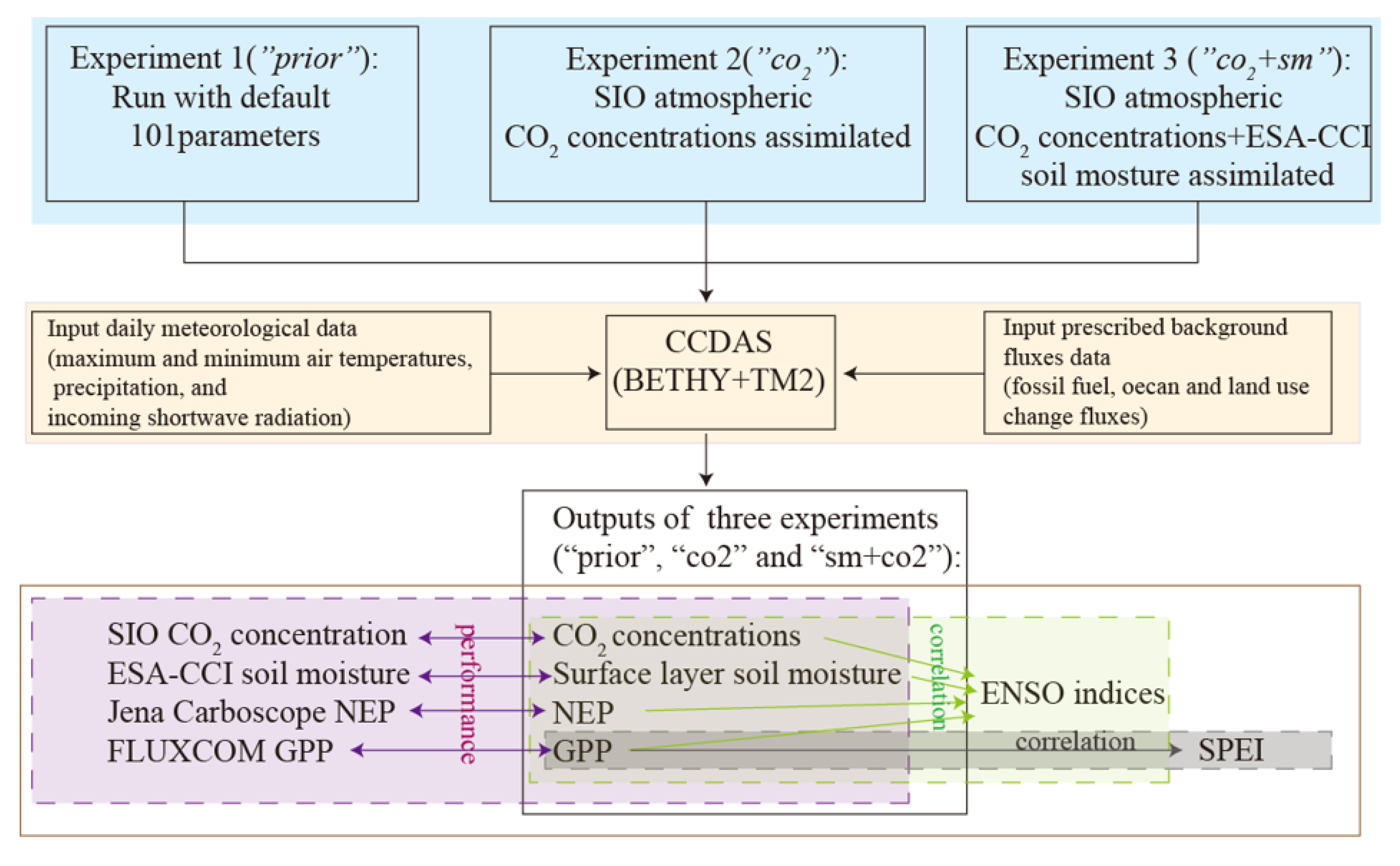
2.1. Carbon Cycle Data Assimilation System (CCDAS) and Simulation Experiments

A Carbon Cycle Data Assimilation System (CCDAS) was used to optimize ecosystem fluxes in this study. CCDAS is based on the BETHY model and combined with an atmospheric transport model (TM2 [51]). CCDAS utilizes a variational method to optimize the process parameters as well as variables by assimilating in situ and remotely sensed observations. The BETHY model simulates carbon cycling as well as the water and energy balance in an ecosystem. Plants are categorized into 13 plant function types (PFTs) and each grid can be represented by at most 3 PFTs, which sum up to be 100% coverage of the area in the grid [19]. Photosynthesis is simulated with the Farquhar equation and C3 and C4 are separately modeled. Soil hydrology is represented by a two-layer bucket model [22] and the first layer which is 4 cm thick corresponds to the soil layer detected by the microwave remote sensing techniques.

Net ecosystem exchange (NEE) simulated by BETHY was then used as an input together with prescribed background fluxes (fossil fuel, ocean and land use change fluxes) for the TM2 [19], which simulates atmospheric CO₂ concentrations at the flask sample stations from National Oceanic and Atmospheric Administration (NOAA) observation networks (NOAA CO₂ networks). The fossil fuel fluxes were from Marland, et al. [52] for the year 1980, and a scaling factor was used for each year from 1981 to 2015 based on ratios of the global annual total fluxes from the Global Carbon Budget (GCB, [53]) to the those by Marland, et al. [52] in 1980. The ocean fluxes were taken from two sources. The fluxes from Takahashi, et al. [54] were used to describe the flux climatology, and we added the anomalies derived from the inversed ocean fluxes with atmospheric TM3 [55] for 1980–2015. For land use change fluxes, we used the flux from 1980 by Houghton, et al. [56] and rescaled it to the other years based on the ratios of the annual total land use change fluxes estimated from GCB to the values from 1980 at the respective grid.

Three experiments were conducted with CCDAS: a ”prior” simulation experiment with default model parameters, a “co₂” simulation experiment with atmospheric CO₂ concentrations from 8 stations (Table A1) assimilated, and a “sm + co₂” simulation experiment with surface soil moisture data from ESA-CCI and atmospheric CO₂ data from 8 stations simultaneously assimilated. The simulation period is 1980 to 2015, with daily soil moisture and monthly carbon fluxes (GPP, NEP, and CO₂ concentrations) as output. The spatial resolution for the simulations is 8° × 10° both for BEHTY and TM2.

In total, CCDAS optimizes 101 parameters related to different processes and different PFTs and soil textures using a variational method which minimizes the cost function with the Broyden–Fletcher–Goldfarb–Shanno (BFGS) method [57]:

J (x) = \frac{1}{2} [\begin{matrix} {(M_{c o 2} (p) - O_{c o 2})}^{T} C_{c o 2}^{- 1} (M_{c o 2} (p) - O_{c o 2}) + \\ {(M_{s m} (p) - O_{s m})}^{T} C_{s m}^{- 1} (M_{s m} (p) - O_{s m}) + \\ {(p - p_{0})}^{T} C_{p}^{- 1} (p - p_{0}) \end{matrix}]

(1)

where M and O stand for model and observation, respectively; subscripts co₂ and sm stand for atmospheric CO₂ concentrations and soil moisture, respectively; C stands for the uncertainty covariance matrices for observations and parameters; p stands for the parameters; p₀ denotes the prior control vector.

2.2. Data

2.2.1. Meteorological Data

Daily meteorological data are input by BETHY and include maximum and minimum air temperatures, precipitation, and incoming shortwave radiation. Here, we used Climatic Research Unit—National Centers for Environmental Prediction (CRUNCEP) v7 [58] and re-gridded the data from the original 0.5° × 0.5° to the 8° × 10° CCDAS spatial resolution. The CRUNCEP is specifically designed to force the land surface models (CLMs) over a long period. The CRUNCEP has been successfully used to drive CLM for vegetation growth, evapotranspiration, and gross primary production and for the TRENDY (trends in net land–atmosphere carbon exchange over the period 1980–2010) project.

2.2.2. Atmospheric CO₂ Concentrations

The atmospheric CO₂ concentrations from 8 flask sample stations were used for assimilation. These 8 stations contain monthly CO₂ concentrations from 1980 to 2015 and are derived from the Scripps Institution of Oceanography (SIO) networks [59]. The CO₂ concentrations at each station were then simulated by the TM2 using terrestrial and background fluxes as inputs.

We computed the global CO₂ growth rate (CGR) based on the CO₂ concentrations from Mauna Loa (MLO) and the South Pole (SPO) and assigned a weight of 0.75 and 0.25 to them, respectively, as done in [19]. We then computed the monthly growth rate as the difference between the de-seasonalized CO₂ concentrations from the next month and the current month, and filtered the data using a 7-month rolling mean method.

2.2.3. ESA-CCI Soil Moisture

The European Space Agency Climate Change Initiative (ESA-CCI) soil moisture dataset was used in the assimilation experiment. This dataset combines observations from active/passive microwave remote sensing products and generates a spatial/temporal continuous daily surface soil moisture product with original spatial resolution of 0.25° × 0.25° [60,61]. Since CCDAS is run at the 8° × 10° grid in this study for efficiency in computing, we re-gridded the soil moisture data to the model resolution. To keep as much useful information from the soil moisture product as possible, we used soil moisture derived from the ‘prior’ simulation experiment to correct the inter-annual variability of the ESA-CCI product. The goals of this bias correction method were to (1) eliminate the requirement for precise texture data and (2) preserve as much pertinent data from the ESA-CCI measurement as is practical. Details can be seen in [22].

2.2.4. GRACE-REC TWS Data

Gravity Recovery and Climate Experiment—REConstruction Total Water Storage (GRACE-REC TWS) data are a statistical reconstruction of GRACE observations from 2002 to 2017. Thorough explanations of the statistical methodology used to produce the reconstruction of historical TWS anomalies may be found in [62]. In conclusion, past changes in water storage were reconstructed using a statistical model that was induced using daily anomalies in temperature and precipitation. The GRACE-REC TWS data we used here were from 1980 to 2015 at 0.5° × 0.5°. We then re-gridded them into 8° × 10° resolution for comparison with CCDAS GPP and other variables from CCDAS.

2.2.5. Top-Down Net Ecosystem CO₂ Flux

The atmospheric inversed monthly net ecosystem exchange (NEE) fluxes from Jena CarboScope (s76oc_v4.3, update of [63,64]) were compared with the optimized NEP from CCDAS. The s76oc_v4.3 product estimates spatially and temporally explicit CO₂ fluxes between the Earth’s surface and the atmosphere using a linear Bayesian inversion approach based on atmospheric CO₂ measurements from 9 stations, each of which spans the entire period from 1976 to 2018. Since the spatial resolution for Jena CarboScope is 3.75° × 5°, we re-gridded the NEE into 8° × 10° and converted it to NEP by minus one.

2.2.6. FLUXCOM Gross Primary Productivity

The upscaled GPP based on FLUXNET2015 [65], denoted as FLUXCOM, was compared with the optimized GPP from CCDAS. The FLUXCOM GPP was developed with a representativeness-based upscaling approach using flux sites that sampled in similar environmental conditions. Strong reflections of the spatiotemporal variability in the distribution of flux observations may be seen in the spatiotemporal variability and accuracy of the upscaled GPP dataset. Because the accessible flux sites provide a good sample of the ecoregions, the dataset has higher accuracy and lower uncertainty in those areas. This product has the spatial resolution of 0.5° × 0.5° and was therefore re-gridded to the CCDAS resolution. We only used the available data from 1982 to 2011 for comparison.

2.2.7. Standardized Precipitation-Evapotranspiration Index (SPEI)

The standardized precipitation-evapotranspiration index (SPEI, [66]) is a drought index that defines the monthly difference between precipitation and potential evapotranspiration (PET). For each grid, we used the multi-year mean value and the Mann–Kendall trend to determine the wet/dry conditions. If the grid has a negative multi-year mean SPEI and a negative trend in SPEI from 1980 to 2015, it is taken as a dry grid that is becoming drier; for a grid with positive multi-year mean SPEI and a positive trend in SPEI, it is taken as a wet grid that is becoming wetter; otherwise the grid is either dry that is becoming wetter or wet that is becoming drier. In determination of the optimal drought duration that can be captured by CCDAS when soil moisture is assimilated, we calculated the correlation between the optimized GPP and SPEI for each grid where the multi-year mean SPEI and GPP anomalies were negative and repeated this 12 times for SPEI derived from different durations (1, 3, 6, 9, 12, 15, 18, 21, 24, 30, 36, 48 months). Finally, the optimal month was determined as the one with the tightest correlation to GPP during droughts.

2.2.8. TRENDY GPP

We used the mean GPP simulations from the TRENDYv6 [16,67] ensemble of TBMs to calculate the correlation with SPEI and evaluate the response of GPP to drought in this study. Climate variability and the observed global CO₂ concentration from the CRUNCEP dataset are used to constrain the TRENDY models. Since the atmospheric CO₂ concentrations in the S3 simulation were based on observation, and the climate and land cover were varied over the modeling period (1980–2015), we primarily analyzed model findings from that simulation. All monthly GPP from TRENDY models were first resampled to 8° × 10° grid in the unit of gC m² yr⁻¹.

2.2.9. GIMMS NDVI

The normalized difference vegetation index (NDVI) is a widely used remote sensing index and is used to describe vegetation greenness. It is calculated as the difference between visible and near-infrared reflectance of vegetation. The latest version (3 g.v1) of the Global Inventory Modeling and Mapping Studies NDVI (GIMMS NDVI) dataset was used to calculate the correlation with SPEI in this study [68,69]. This long-term NDVI time series (8 km pixel size, available twice monthly) spans the period July 1981 to December 2015. This dataset was created using reflectance data obtained from the GIMMS project using channels 1 and 2 of the Advanced Very High Resolution Radiometer (AVHRR). This product was re-gridded to the CCDAS resolution.

2.2.10. LT_SIF

The solar-induced chlorophyll fluorescence (SIF) data called LT_SIF from [70] were used in this study. The LT_SIF was developed to correct the temporal inconsistencies in the far-red SIF data from various satellites (GOME, SCIAMACHY, and GOME-2) using the time series of SIF data from the Sahara Desert as the benchmark. The three satellite sensors’ distinct time series of SIF data were then combined to create LT_SIF, which stands for Long-Term Consistent Global SIF dataset and spans the period from July 1995 to December 2018 (termed as LT_SIF). We re-gridded the LT_SIF into 8° × 10° and only used the available data from 1995 to 2015 to calculate the correlation with SPEI.

2.2.11. ENSO Indices

The El Niño/Southern Oscillation (ENSO) is used to represent the changes in the equatorial Pacific Ocean and is the main factor of global climate change. ENSO indices are used to characterize the intensity of an ENSO event. Two ENSO indices were selected to represent the El Niño-Southern Oscillation. The first one is the Multivariate ENSO Index (MEI.v2, [71,72,73]). It is calculated every two months by combining the Empirical Orthogonal Function (EOF) of five different variables (sea level pressure, sea surface temperature, zonal and meridional surface wind, and outgoing longwave radiation over the tropical Pacific basin in the area between 30°S and 30°N and 100°E and 70°W). The second one is the Niño 3.4 [74], representing the average equatorial sea surface temperature (SST) in the region 5°N-5°S and 170°W-120°W. These two indices were de-seasonalized and normalized by their mean values and standard deviations, respectively.

Strong El Niño/La Niña events are defined when the ENSO index anomaly is larger than 1 or smaller than −1 for more than six continuous months. Additionally, for each ENSO index, we put the moderate-to-strong El Niño events (anomaly > 1) and moderate-to-strong La Niña events (anomaly < −1) together for calculation of the correlations between soil moisture, NEP, CGR, and ENSO, as well as for estimates of the differences in these variables between El Niño and La Niña events in different continents. The neutral ENSO events are then defined as the absolute value of the ENSO index being smaller than 1.

2.3. Statistical Analysis

The trend for the data in this study was computed using the Mann–Kendall method and the significance was derived simultaneously. The Pearson correlations were used to determine the correlations between different datasets and significance values were simultaneously obtained.

Since this study focused on the inter-annual variability (IAV) of carbon–water couplings on a continental scale, which was much larger than the CCDAS original resolution (e.g., 8° × 10°) and other models and products (e.g., 0.5° × 0.5° to 2° × 3°), we mainly validated our results on their representation of the IAV from different latitude bands or on a global scale and used the power spectra to conduct the validation.

CCDAS time series outputs including GPP, NEP, and soil moisture from three experiments (‘prior’, ‘co₂’, and ‘sm + co₂’) aggregated from different latitude bands, i.e., 60°S–30°S, 30°S–0°, 0°–30°N, 30°N–60°N, 60°N–90°N, were transferred to the frequency domain using the Fast Fourier transform (FFT) package in MATLAB [75] after removing inter-annual variability. The derived variables were then depicted with a relationship between power and period.

2.4. Evaluation Metrics

In this study, root mean square error (RMSE) was used to evaluate the performance of the assimilation. Each output (CO₂ concentration, surface layer soil moisture, NEP, and GPP) of the model employed RMSE with its corresponding observation (SIO CO₂ concentration, ESA-CCI soil moisture, Jena CarboScope NEP, and FLUXCOME GPP).

RMSE = \sqrt{\frac{1}{N} \sum_{i = 1}^{N} {(O (i) - M (i))}^{2}}

(2)

where N is the total number of observations, O is the observed value, and M is the simulated value.

Another correlation coefficient of determination (R²) was employed to assess the representativeness of model outputs to inter-annual variability and the GPP response to drought.

R^{2} = 1 - \frac{\sum_{i = 1}^{N} {(O (i) - M (i))}^{2} / m}{\sum_{i = 1}^{N} {(O (i) - \bar{M})}^{2} / m}

(3)

Figure 1 shows the framework of methodology in this study. The calculation of these evaluation metrics and other unspecified data analysis tasks such as pre-processing and post-processing of data were all performed in python.

3. Results

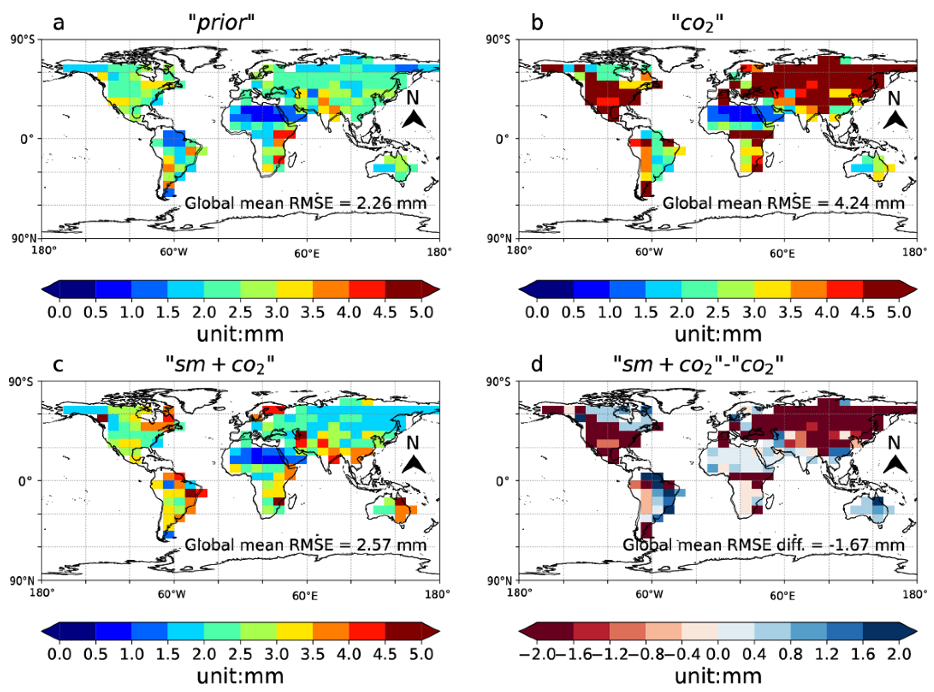
3.1. Soil Moisture Assimilation Performance

As seen in Figure A1, in the “prior” experiment, the difference between the simulated CO₂ concentration results and the observations gradually grows with increasing simulation time. This issue is resolved in the “co₂” and “sm + co₂” experiments, where the optimized CO₂ concentrations are closer to the observations. Table 1 displays the RMSEs of these three experiments. For each of the eight flask sampling stations, the “sm + co₂” simulation demonstrates large improvements in the simulated atmospheric CO₂ concentrations compared with the prior simulations. Assimilation of CO₂ concentrations and ESA-CCI soil moisture lowers RMSE from 15.56 and 15.77 ppm for “prior” to 1.13 and 0.89 ppm for “co₂” and 0.89 and 0.31 ppm for “sm + co₂” experiments at BHD and SMO sites, respectively. At the CHR site, the RMSE obtained for the “sm + co₂” experiment was identical with that of the “co₂” experiment, both at 1.12 ppm. As expected, slightly higher RMSE values than the “co₂” experiment were recorded at some sites. At the ALT, BRW, KUM, MLO, and SPO stations, the “sm + co₂” achieves the RMSE of 2.07, 2.54, 1.77, 1.42 ppm, and 1.29 ppm, respectively; whereas in the “co₂” experiment, the RMSE is 1.54, 1.71, 1.28, 0.97 ppm, and 0.80 ppm, respectively.

In Figure 2, the comparison between simulated surface layer soil moisture content from three experiments and the ESA-CCI observations is displayed. The global mean soil moisture RMSE decreases from 4.24 mm for “co₂” experiments to 2.57 mm for “sm + co₂” experiments as a result of the simultaneous assimilation of CO₂ concentrations and ESA-CCI soil moisture, respectively (Figure 2 b,c). The global mean soil moisture RMSE for “sm + co₂” is slightly higher than the “prior” RSME of 2.26 mm (Figure 2a). Reductions from “co₂” to “sm + co₂” experiments are shown for mainly north of the 30°N latitude, with overall values reduced by −1.67 mm globally, but with a little degradation in tropical regions (Figure 2d).

In the “co₂” simulation and the “sm + co₂” simulation, the global mean RMSE of the simulated NEP is reduced from 23.55 gC/m²/month in the “prior” simulation to 22.95 gC/m²/month and 21.93 gC/m²/month (Figure 3a–c). Middle and high latitudes of Eurasia and North America, where an RMSE decline in NEP primarily occurs, are where soil moisture has also shown large improvements (Figure 3c). In areas such as the Amazon, Sahara, and Australia, where soil moisture is not greatly enhanced, a slight increase in RMSE can be seen. For GPP, the global mean RMSE values decreased from 68.60 gC/m²/month to a value of 57.76 gC/m²/month in “sm + co₂”, a 13.41% decline (Figure 3a,d), whereas in the “co₂” experiment, the RMSE is 68.68 gC/m²/month. In most regions, the RMSE for GPP has been reduced rather greatly, particularly in the Amazon, Africa, North America, Central Europe, and Australia. When the ESA-CCI soil moisture is added in the “sm + co₂” experiment, the model performs better in modeling both soil hydrology and CO₂ concentrations, as shown in Figure 2 and Figure 3.

3.2. The Inter-Annual Variability of the Carbon and Water Fluxes

The correlations between the simulated variables from three experiments (“prior”, “co₂”, and “sm + co₂”) and moderate-to-strong ENSO events were used to depict the model performance in representing the inter-annual variability at global scale. Our results suggest that the “sm + co₂” experiment obtained the correlations between soil moisture anomalies from 30°N to 60°N (others are detailed shown in Figure A2) and MEI/Niño 3.4 (Figure A3a) of 0.78/0.76 (p < 0.001), respectively (Figure A3b), with a time lag of 3 months (Figure A4a). The correlations between the “sm + co₂” optimized NEP anomaly and MEI/Niño 3.4 are −0.60/−0.64 (p < 0.001, Figure A3c), respectively. The time lags of the “sm + co₂” optimized NEP and the Jena CarboScope inversed NEP to MEI/Niño 3.4 are 6 months and 8 months, respectively (Figure A4b). The optimized global CO₂ growth rate (CGR) shows the correlation with the MEI/Niño 3.4 as 0.52/0.41 (p < 0.001), respectively (Figure A3d), with a time lag of 5 months (Figure A4c). The CCDAS-optimized GPP from 30°N to 60°N shows tighter correlation to the two ENSO indices than the FLUXCOM GPP (−0.29/−0.39 vs. 0.01/−0.05, p < 0.001, Figure A3e and Figure A5b).

In Figure A6, we presented the power spectrum of the CCDAS output variables, e.g., GPP, NEP, and surface soil moisture (0–5 cm). The power spectra show the features of variability of GPP, NEP, and soil moisture in the frequency domain. Overall, the ENSO-band variations of all variables are characterized by a relatively larger amplitude at low/mid latitudes (e.g., 30°N-60°N and 0–30°S) and a smaller amplitude at high latitudes (60°N-90°N).

CCDAS-optimized surface soil moisture (0–5 cm) and GPP show contrasting relations over the six continents (Figure 4a,b). Overall, for North America, Europe, and Asia, which are mainly north of 30°N, all aggregated moderate-to-strong El Niño/La Niña events result in lower GPP but higher soil moisture, while for South America, Africa, and Oceania, which are mainly south of 30°N, all aggregated moderate-to-strong El Niño/La Niña events result in the same trend of GPP and soil moisture. GPP decrease during moderate-to-strong and strong El Niño events in Asia (−0.26/−0.39 PgC yr⁻¹) and Europe (−0.23/−0.20 PgC yr⁻¹) is accompanied by an increase in surface soil moisture (0.32/0.23 × 10⁻¹ mm and 0.26/0.29 × 10⁻¹ mm, respectively). In North America, an increase in GPP during moderate-to-strong and strong El Niño events (0.20/0.34 PgC yr⁻¹) is mainly caused by an increase in surface soil moisture (0.52/0.68 × 10⁻¹ mm). In South America, the El Niño events contribute to an increase in GPP (0.90/1.00 PgC yr⁻¹) accompanied by an increase in surface soil moisture (0.88/0.95 × 10⁻¹ mm). In South Africa and Oceania, a decrease in GPP during El Niño (−0.47/−0.59 PgC yr⁻¹ and −0.43/−0.33 PgC yr⁻¹) is accompanied by a positive surface soil moisture anomaly (−0.57/−0.86 × 10⁻¹ mm and −1.47/−0.95 × 10⁻¹ mm).

A linear relationship between GPP anomalies and TWS anomalies (Figure 4c) is obtained for all continents except South America during moderate-to-strong and strong El Niño/La Niña events (r = 0.85). We notice that in four out of the six continents (e.g., Asia, Europe, Africa, and Oceania) defined in Figure A7, El Niño results in a decrease in GPP, while La Niña results in an increase in GPP. In North America, both El Niño and La Niña contribute to an increase in GPP. South America shows a contrasting relationship between GPP and TWS, with an increase in GPP and an increase in TWS during El Niño, and a decrease in GPP and a decrease in TWS during La Niña.

3.3. Drought Impacts on Continental GPP

The tightest correlation between the optimized GPP from CCDAS and SPEI among 12 drought durations (1, 3, 6, 9, 12, 15, 18, 21, 24, 30, 36, 48) was identified as the optimal drought duration. The percentage of droughts of 9 months’ duration identified by the CCDAS-optimized GPP was 48%, which is the maximum among 12 durations (Figure 5a). Additionally, a total of 68% of droughts of less than 9 months’ duration were identified by the CCDAS-optimized GPP. This suggested that the CCDAS could better capture the response of GPP to sub-annual drought durations (less than 9 months) by assimilating both CO₂ and soil moisture. The TRENDY GPP had the highest percentage at the 48-month drought duration with 34% (Figure 5b) and the percentage of 80% for droughts greater than 12 months’ duration, which showed that TRENDY GPP was not good at capturing sub-annual drought durations (9 months and below) but could capture long-term drought durations (12 months and above) very well. Similar to TRENDY, GPP proxies NDVI and SIF derived from remote sensing also had the highest percentages at 48 months with 22% and 31% (Figure 5c,d), as well as the total percentages of 66% and 77%, respectively, for droughts of a duration greater than 12 months. Since CCDAS identified the 9-month drought duration best, the next analyses related to SPEI were based on SPEI-9.

The spatial distributions of drought-aggregated GPP anomalies for CCDAS and TRENDY and NDVI anomalies for GIMMS3g from SPEI-9 with SPEI < –1 were similar in most areas (Figure 6). As can be seen in Figure 6a–c, CCDAS, TRENDY, and NDVI all show a trend of reduced vegetation growth (decreased GPP and NDVI) when drought occurs in most areas south of the 30°N latitude. For most regions north of 30°N, especially northern North America and northern Asia, both CCDAS GPP and NDVI show a trend of increased vegetation growth (increased GPP and NDVI) when drought occurs, but TRENDY shows a trend of a decrease in these regions. Further, the CCDAS-optimized GPP showed a weak increase in the Amazon rainforest region (Figure 6a), which is in agreement with TRENDY (Figure 6b), but disagreement with NDVI and SIF, which show lower values in the tropical rainforest region (Figure 6c,d). That is, the CCDAS-optimized GPP showed that GPP increased in mid- and high-latitude regions in response to drought and weakly decreased in tropical rainforest regions (Figure 6a).

To further prove the rationality of the CCDAS results, we calculated the correlation between the CCDAS-optimized GPP and SPEI-9 as well as the region of drought changes identified using SPEI-9. The CCDAS-optimized GPP showed a positive correlation in the southern parts of North America and South America as well as western parts of Asia, where it became drier from dry (DD) and drier from wet (WD), which was identified by SPEI-9 (Figure 7), suggesting that GPP decreases with more severe drought and results in decreased GPP in these areas. It is noteworthy that tropical rainforest areas also showed a change from dry to drier (DD) and the correlation coefficient between GPP and drought also showed a slight negative correlation, which demonstrated that water reduction brings higher GPP instead in the Amazon rainforest region. The negative correlation between GPP and drought was concentrated in mid- and high-latitude regions, suggesting that moisture is not a major limiting factor in these regions, such as the northern parts of Asia, Eurasia, and North America, where the melting of snow and ice due to climate warming had led to a change from dry to wet (DW) or wet to wetter (WW).

4. Discussion

4.1. The Mechanism of Soil Moisture Controls on Carbon Fluxes

Photosynthesis, heterotrophic respiration, C pool size, and phenology are all controlled by CO₂ and it makes sense that when only assimilating the atmospheric CO₂ concentrations, performance is better than when simultaneously assimilating CO₂ concentrations and soil moisture. According to Scholze, et al. [22], the soil moisture affects the water uptake and surface energy balance and assimilating satellite-derived soil moisture constrains the model’s phenology and photosynthesis. In actuality, the model’s hydrological scheme’s process parameters are corrected by assimilating the surface soil moisture. Since surface and root zone soil moisture share common parameters, such as soil porosity, which is used to calculate soil water properties, through these parameters, the assimilation of satellite-derived surface soil moisture also controls plant-available soil moisture. When simultaneously assimilating atmospheric CO₂ and soil moisture, parameters such as

V_{c m a x}

, Tϕ, Cw0, srdepth, Sb, emis0, and Offset (regulating the soil water and energy balance, Table A2) are additionally constrained. Here, the carbon fluxes are further constrained by the ESA-CCI soil moisture observations. Modulated by ENSO variability on inter-annual time scales, the simulated soil moisture, NEP, GPP, and CGR showed tighter correlation to the ENSO indices especially from 30° N to 60° N. That is, when assimilating both CO₂ and ESA-CCI data simultaneously, the optimized CCDAS can be used to better present the inter-annual variability of carbon–water couplings on large scales and the assimilation of satellite soil moisture observations helps to achieve a better representation of carbon processes in addition to soil hydrology. Our finding is consistent with Wu, et al. [23], who showed that remotely sensed soil moisture assimilation provided better a constraint on the global carbon cycle than assimilation of CO2 alone and demonstrated the capabilities of CCDAS to assimilate soil moisture. This is because CCDAS used the strategy of optimizing model parameters and state variables (e.g., Offset) simultaneously, which constrained model parameters related to physiology, phenology, soil hydrology, as well as energy balance and carbon cycle, and by these parameters was able to influence the water uptake and surface energy balance as well as plant-available soil moisture [22,23].

4.2. Legacy in the Regional GPP Variability

Reduced precipitation, continental freshwater discharge [76], and evapotranspiration [77] over most land areas are associated with El Niño, whereas wetter land occurs during La Niña [39]. It is clear that El Niño years induce more droughts and a restricted amount of terrestrial moisture, which increases plant moisture stress through higher moisture demand and the corresponding rise in continental temperature. We show that El Niño results in a decrease in GPP, while La Niña results in an increase GPP, which is consistent with [77,78], who demonstrated that the global terrestrial biosphere reduces in both net and total production with warm ENSO (El Niño) occurrences, but the capacity of the terrestrial carbon sink rises with cool ENSO (La Niña) events. It has proven that the ENSO phases (La Niña, neutral, and El Niño years) strongly impact the vegetation productivity on a continental scale [79].

In this study, we also found that the ENSO shows lagged effects on GPP and varies continently. For the GPP aggregated in each continent as defined in Figure A7, different time lags are obtained. North America, Asia, and Europe (mainly distributed in the Northern Hemisphere) show a >3-month time lag and South America, Africa, and Oceania (mainly distributed in the Southern Hemisphere) show just a <3-month time lag (Figure A8c). A clear lag effect of ENSO indices on global GPP variability was discovered by [80] when they evaluated the effects of ENSO on global GPP dynamics from 1982 to 2016. Our results are similar to those of Vicente-Serrano, et al. [81], which illustrated that South Africa, Australia, and Southeast Asia are the regions most impacted by El Niño phases and, in those regions, dry conditions are observed at the beginning of events over short time scales (1–3 months). However, in large areas of America and Eastern Europe, the effects were more noticeable over longer time scales and were impacted by La Niña phases. Additionally, Bastos, et al. [82] demonstrated that because of the response of the Southern Hemisphere’s ecosystems, notably in tropical and subtropical regions, ENSO explains more than 40% of global net primary production (NPP) variability.

4.3. Drought Impacts on Continental GPP

Drought may significantly affect terrestrial carbon fluxes through the severely impacted structure and function of terrestrial ecosystems [83,84,85]. The factor that primarily regulates vegetative activity affects how GPP reacts to drought. For instance, temperature and radiation are major factors restricting the productivity of terrestrial ecosystems in northern regions of the Northern Hemisphere. [86,87]. In these areas, drought was typically followed by temperature and radiation increases, which may have contributed to a rise in GPP [86,88,89,90]. In our study, except for some regions in high latitudes in the Northern Hemisphere which showed increased GPP when drought happened, parts of tropical South America also showed an increase in GPP. For these regions, GPP showed a negative correlation with drought, which means that when drought occurs, GPP shows higher values. As indicated by Nemani et al., (2003) [86], at high latitudes in the Northern Hemisphere, temperature was the major limitation for vegetative productivity. Decreasing precipitation was typically followed by increasing temperature, which induced increased GPP. Our study is consistent with [30,91], which showed that GPP has increased in some high latitudes of the Northern Hemisphere. With regard to the Amazon rainforest, radiation is the main factor affecting GPP in South America’s tropical regions. [86,87]. In most cases, the reduction in precipitation happened at the same time as the rise in radiation. As a result, in the Amazon rainforest, GPP increased slightly in drought years compared to normal years. Our study is consistent with [92,93], which showed that GPP increased in drought years. However, some studies find that the drought has reduced GPP [94,95]. Therefore, GPP response to drought in rainforests has large uncertainties and needs to be more deeply investigated in the future. The pattern of GPP response to drought in this study is similar to that from the BEPS [96], CABLE, LPJ-wsl, and ORCHIDEE models. This demonstrates that simultaneous assimilation of soil water and CO₂ can effectively reveal the spatial characteristics of drought effects on GPP.

Drought duration is a key variable for describing the large-scale biospheric drought response [30]. In this study, the optimized CCDAS GPP can reflect the effect of sub-annual drought durations (<9 months) on GPP in most of the world (68%) by adding the assimilation of soil moisture, while for GPP products from other process-based TBMs (TRENDY) as well as the NDVI and SIF derived from remote sensing, they capture longer drought durations (>12 months) in most parts of the world. As previously described, daily scale ESA-CCI soil moisture observations were used to optimize model parameters to produce monthly scale carbon and water fluxes, and this daily scale assimilation is able to capture the seasonal and inter-annual variability of water and thus better reflect the short-term drought (<9 months) impacts on GPP. Many studies have been conducted on the relationship between GPP and drought [41,97,98,99,100,101,102,103,104], and the majority of these focused on the outputs of TBMs’ simulations or currently available remote sensing products. In this study, we employed multiple sources of observations, including satellite-derived soil moisture and in situ CO₂ concentrations, to efficiently constrain the parameters of the carbon and water cycle processes through data assimilation techniques. Based on the constrained simulated GPP, we then reliably revealed the differences in GPP response to drought duration at the regional scale.

4.4. Caveats and Implications

Considering the computational capacity of the model and the long assimilation period (36 years), we use the coarse model resolution (8° × 10°) to perform the assimilation experiment. We were able to show and quantify the additional value of the ESA-CCI soil moisture observation as a significant constraint on the terrestrial carbon cycle and could capture the response of GPP to drought at this coarse resolution. Previous studies showed that drought has cumulative effects [100,102,105] and lagged effects on vegetation [99,100,106,107]. SPEI at different time scales calculates the difference between precipitation and PET during the current and previous months [99]. SPEI at different time scales could therefore measure the cumulative effect of drought on vegetation. However, the SPEI with a time scale of 9 months in this study causes difficulty in identifying the lagged effect of droughts on GPP [104]. In addition, it would take a high resolution to accurately capture the lagged effects of drought on GPP [99,104,106], so the coarse spatial resolution in this study makes the analysis of the legacy effects of drought on GPP more challenging. In the future research, the resolution of the assimilation system needs to improve to investigate the lagged effect of specific drought events on GPP at a higher spatial resolution. It is expected that the assimilation of satellite-derived soil moisture observation data would be a promising approach to analyze the cumulative and lagged effects of drought on GPP on finer scales.

It is necessary to further develop the terrestrial biosphere model. For instance, it may be crucial to include more precise processes relating to soil water and heat transfer in soil profiles to the model to improve the model’s response to extremes such as drought. Another option for future research is to continually (i.e., simultaneously assimilation) add new datasets to the model assimilation in order to constrain the processes of the ecosystem model, which are now largely unconstrained. Potential candidate observations include VOD (Vegetation Optical Depth) to provide a constraint on the total amount of vegetation water content and COS (Carbonyl Sulfide) to include a more direct constraint on photosynthesis.

5. Conclusions

In the present study, we used simultaneous assimilation of ESA-CCI soil moisture and atmospheric CO₂ in situ observations to constrain the global terrestrial carbon cycle during 1980–2015 within a Carbon Cycle Data Assimilation System (CCDAS). We demonstrated the importance of soil moisture in the TBMs for terrestrial carbon and water cycles modeling with a CCDAS. The conclusions are as follows:

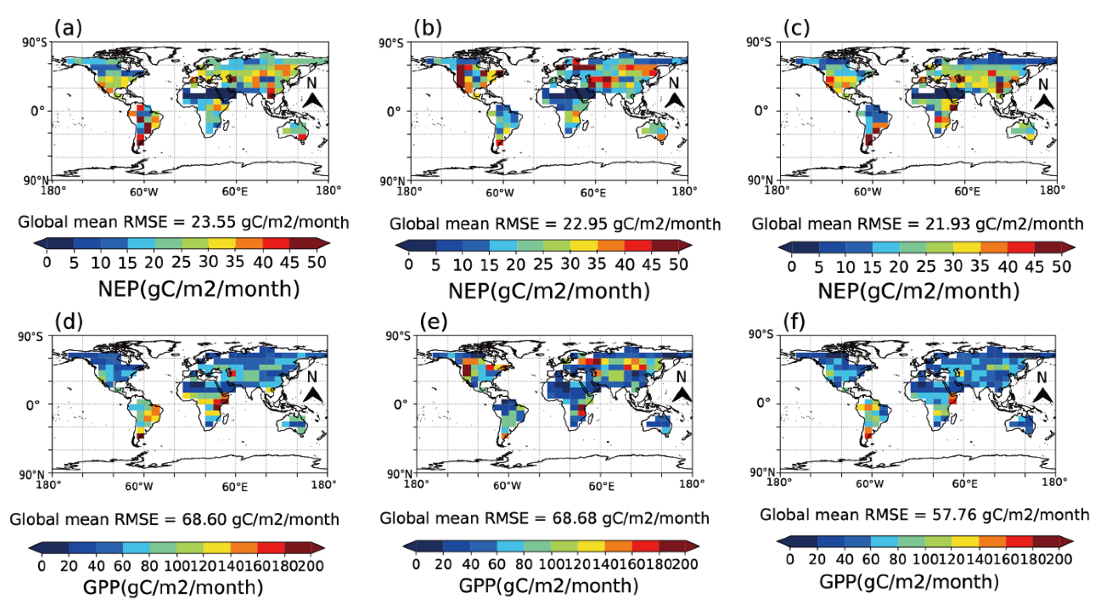
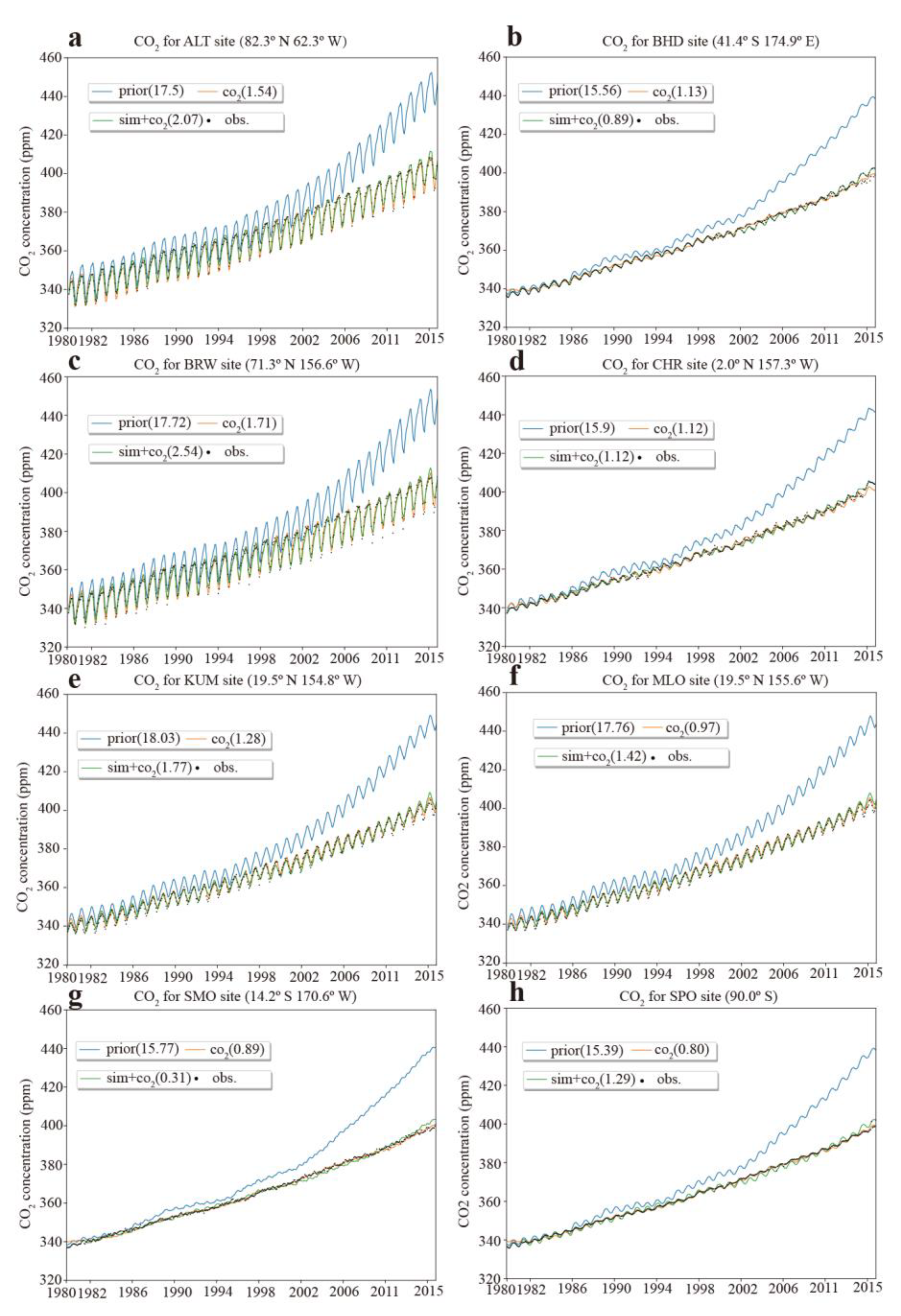
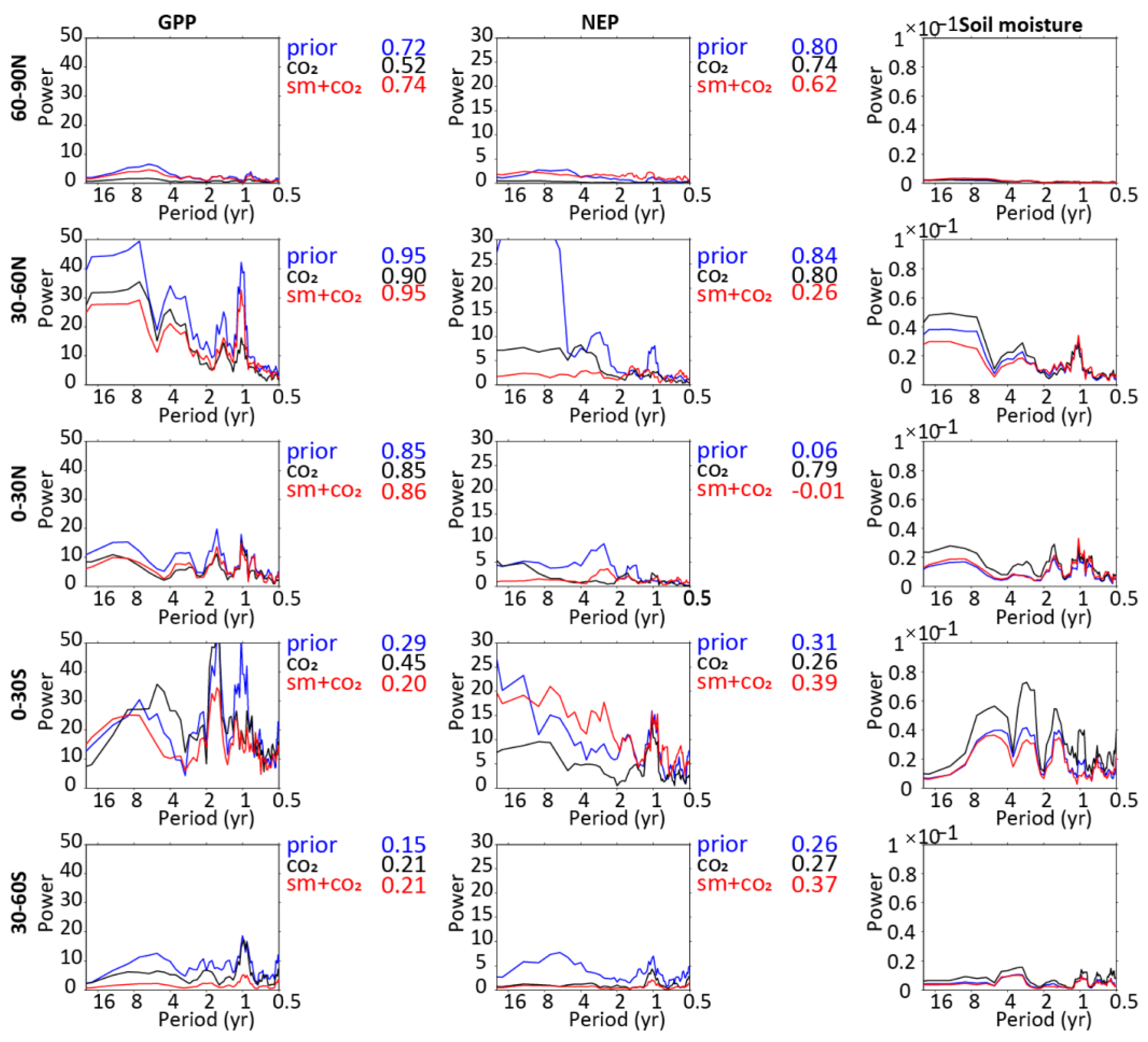
1.: The combination of soil moisture and atmospheric CO₂ concentrations in CCDAS results in a much better simulation of the terrestrial biosphere model in simulating coupled water–carbon processes in ecosystems. For NEP and GPP, the RMSE between the optimized model and Jena CarboScope as well as FLUXCOM is reduced by 6.88% and 14.93% compared to the prior experiment, and by 4.44% and 15.90% compared to only assimilating CO₂. The reason why adding soil moisture observations can better represent the carbon and water cycle is that the soil moisture constrains the model’s phenology and photosynthesis through affecting the water uptake and surface energy balance-related parameters ( $V_{c m a x}$ Tϕ, Cw0, srdepth, Sb, emis0, and Offset) and additionally controls (through these parameters) plant-available soil moisture.
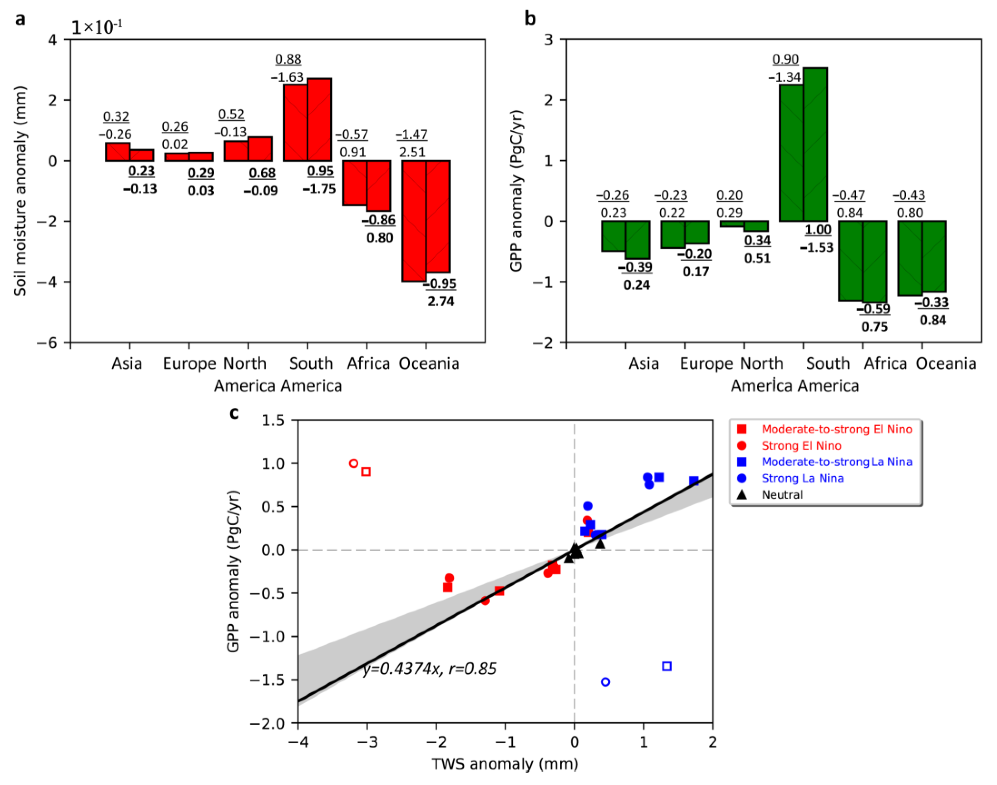
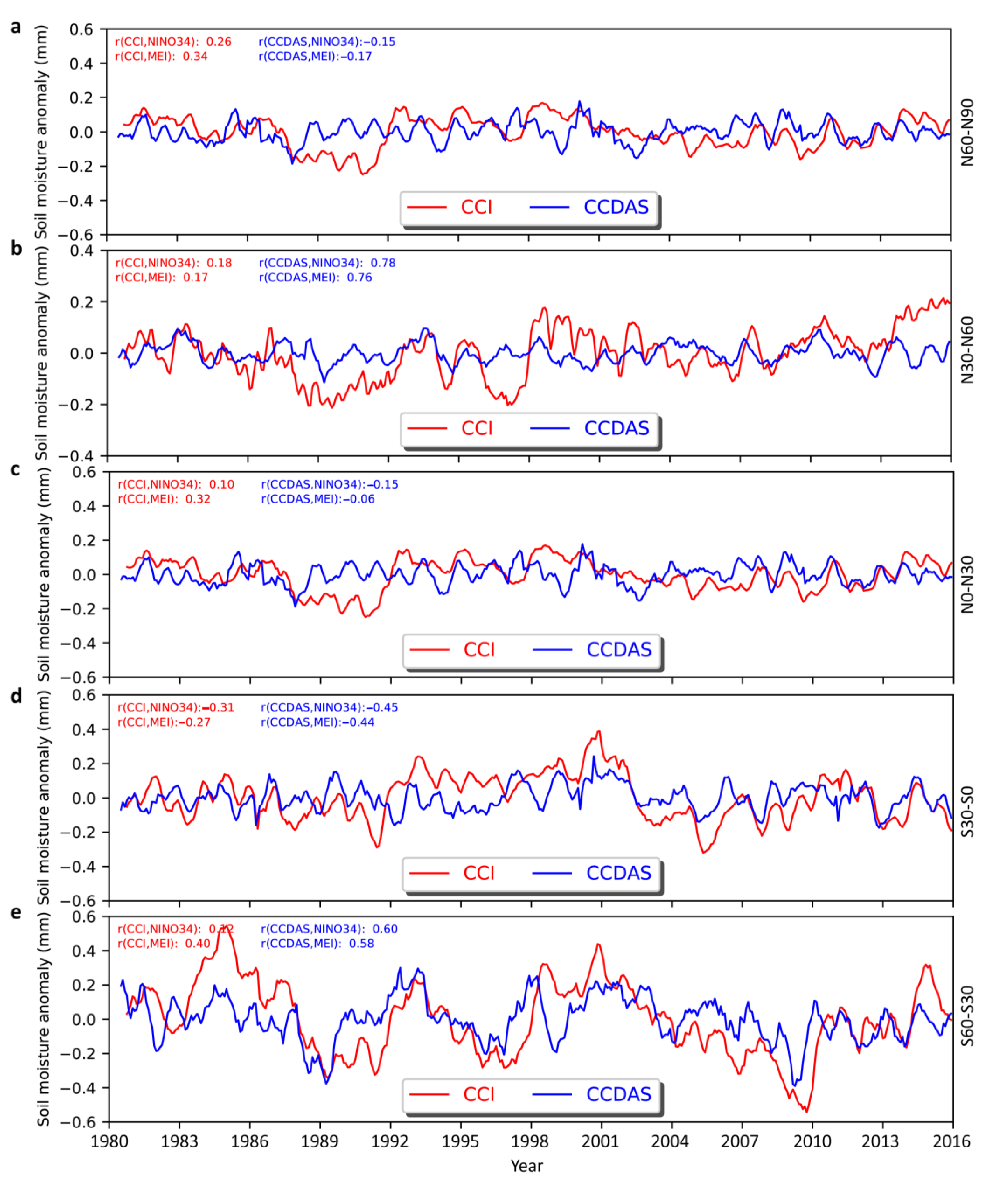
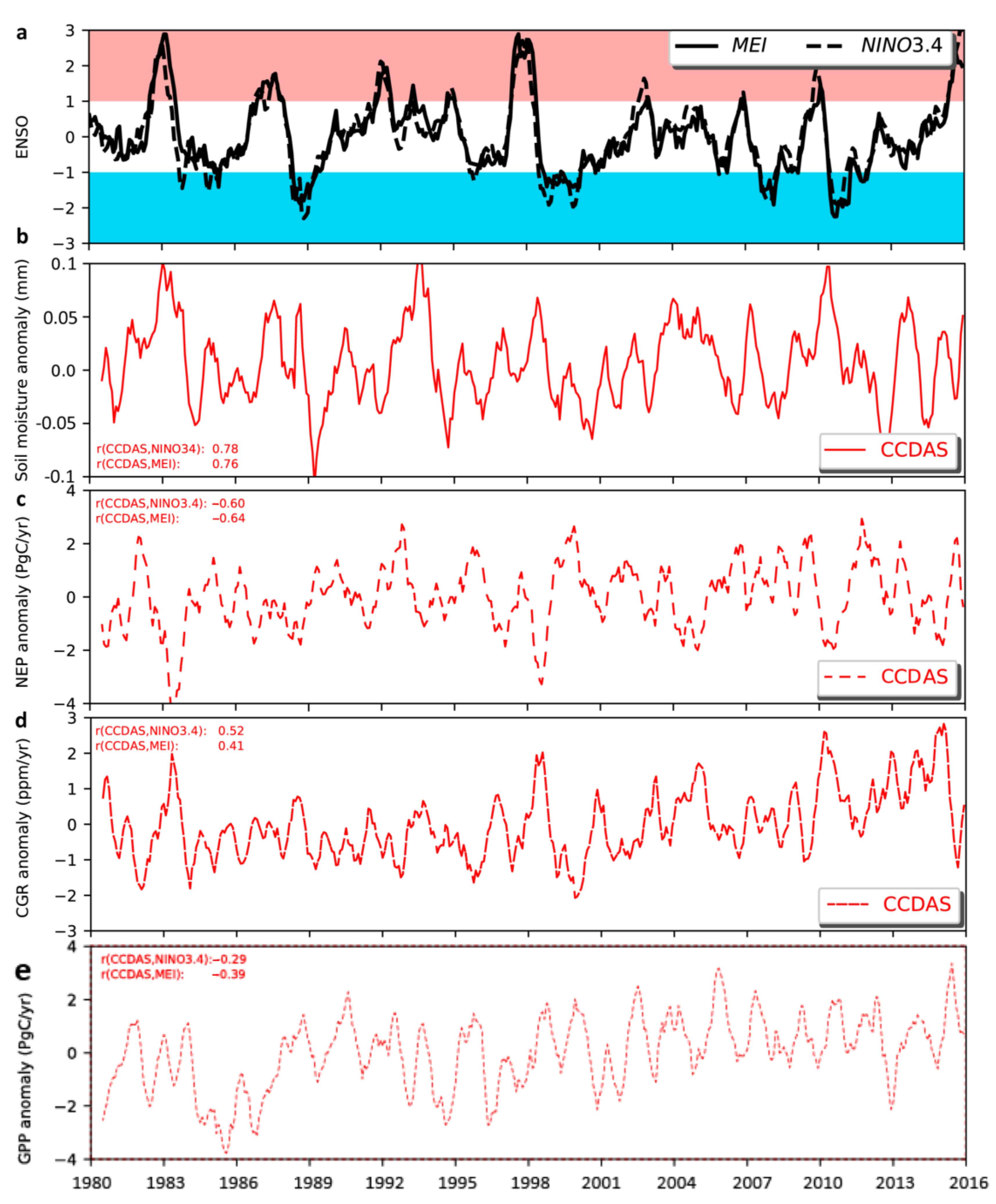
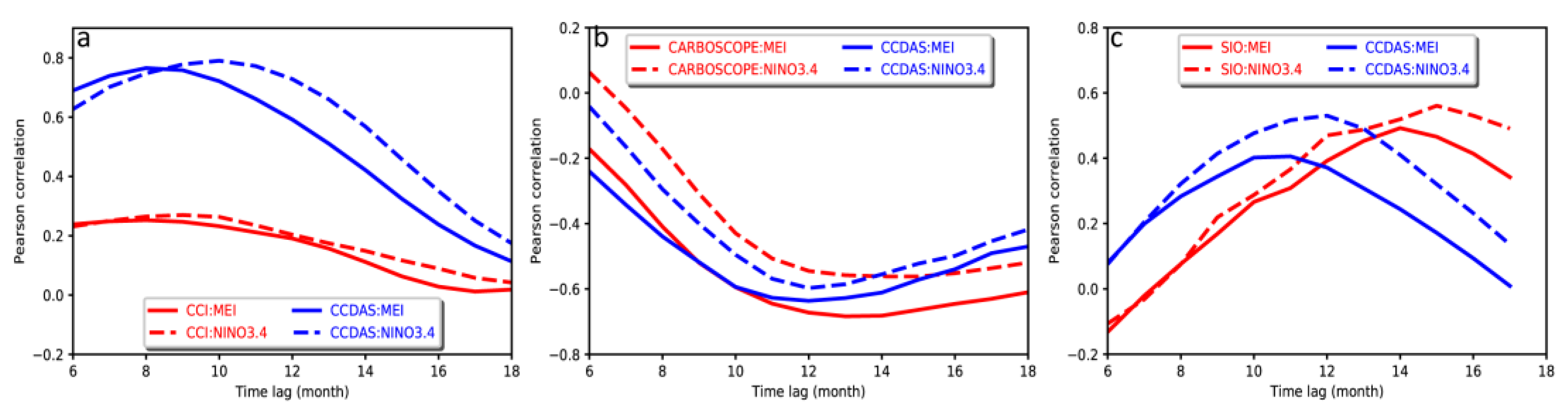
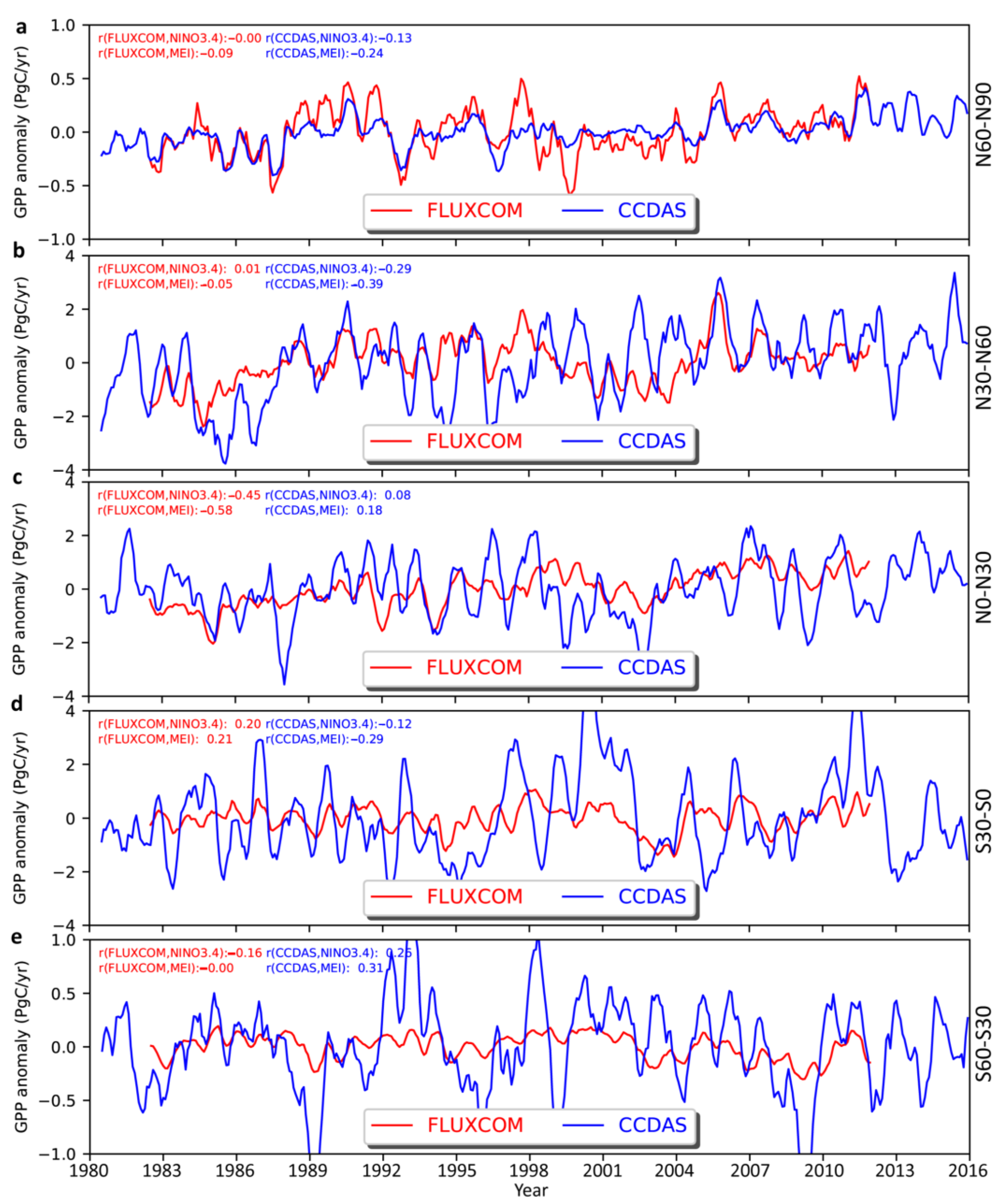
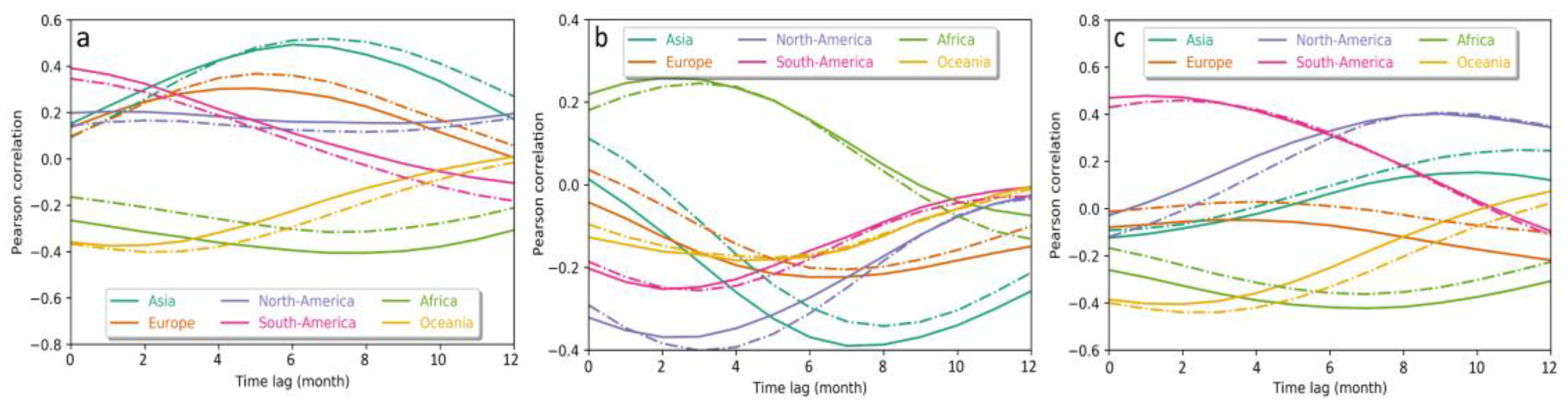
2.: The assimilation of soil moisture has shown the ability of improving the model’s representation of inter-annual variability of terrestrial carbon–water cycles and the atmospheric CO₂ growth rate, resulting in high correlations with ENSO indices (soil moisture: >0.70, NEP: <−0.60, GPP: <−0.20, and CGR: >0.40). Soil moisture is the main factor controlling GPP at the time of ENSO events. For continents mainly distributed north of 30°N (North America, Europe, and Asia), the ENSO results in lower GPP but higher soil moisture, while for continents mainly south of 30° (South America, Africa, and Oceania), ENSO results in the same trend of GPP and soil moisture. We also found that the ENSO shows lagged effects on GPP and varies continently. North America, Asia, and Europe (mainly distributed in the Northern Hemisphere) show a >3-month time lag compared to South America, Africa, and Oceania (mainly distributed in the Southern Hemisphere), which show just a <3-month time lag.
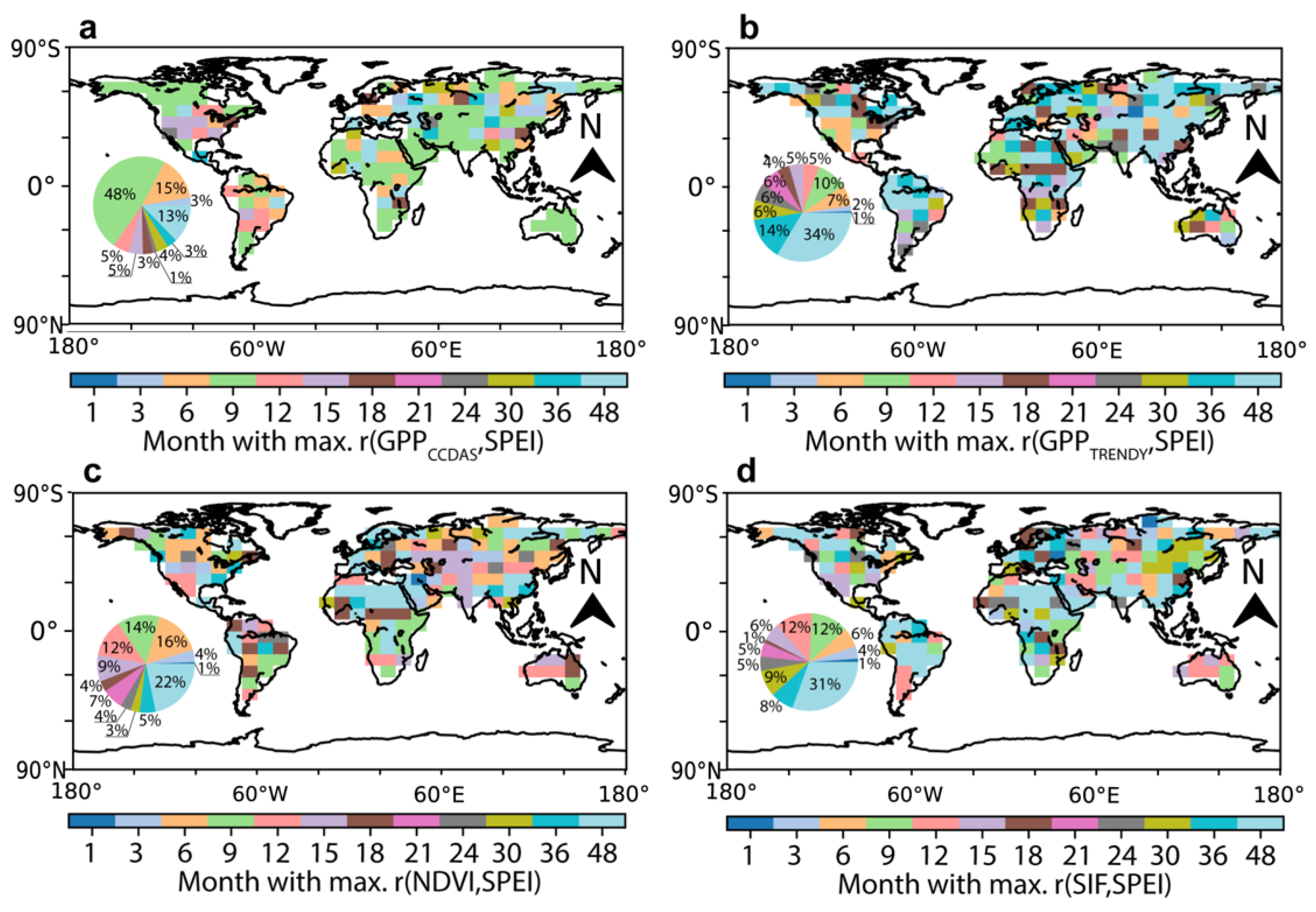
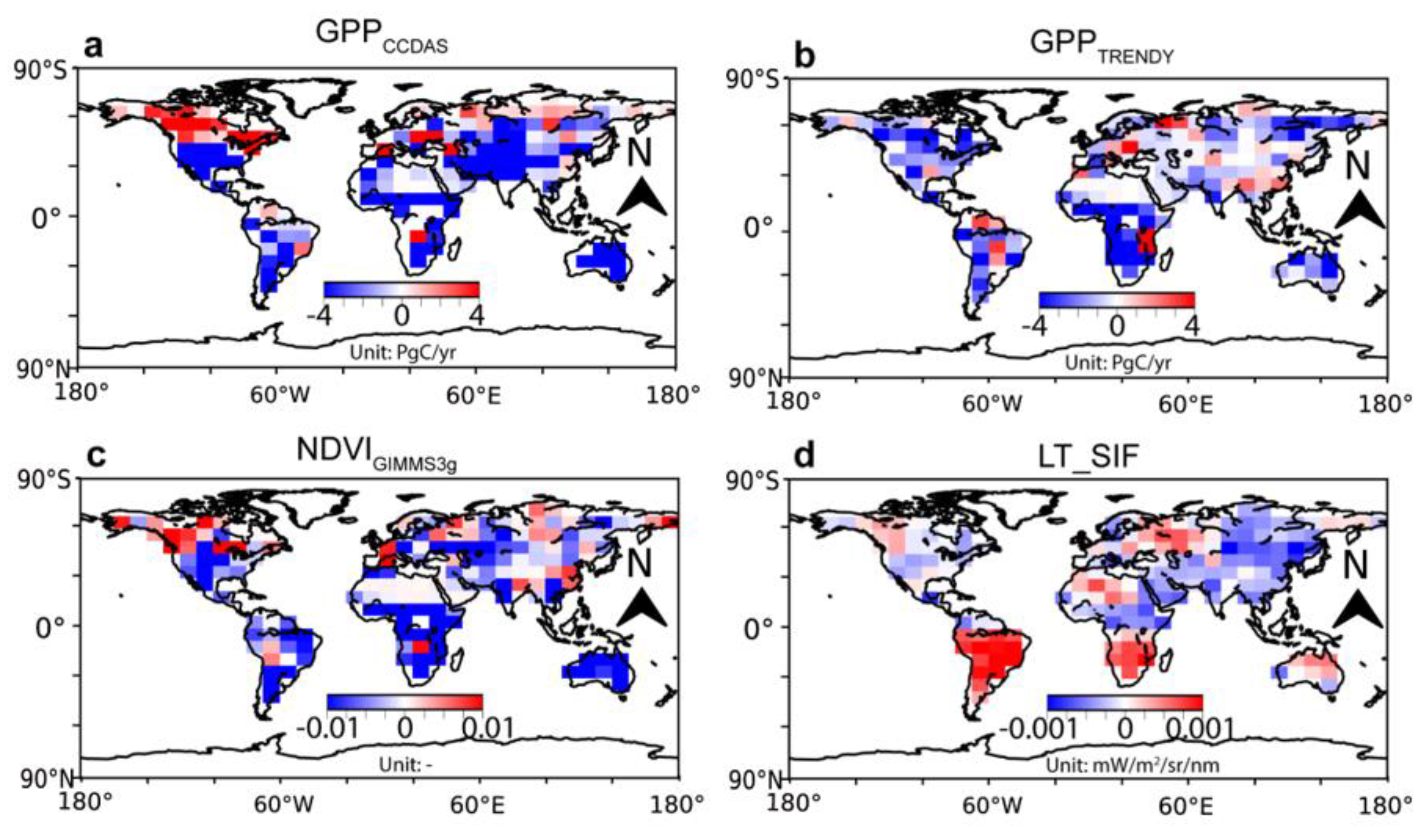
3.: We show that the optimized GPP is capable of reasonably depicting the response of GPP to sub-annual drought (≤9 months) by contrasting the continentally aggregated GPP with the comprehensive drought index SPEI. For the GPP optimized by CCDAS with both soil moisture and CO₂ concentration, GPP responded to 68% of droughts detected globally with less than 9 months’ duration, while for TRENDY GPP, GIMMS NDVI, and LT_SIF, these percentages are 20%, 34%, and 23%, respectively. Based on this 9-month time scale, we analyzed the regional-scale GPP response to drought and showed that for regions at high latitude in the Northern Hemisphere, where temperature is the primary control of drought, an increase in GPP occurs with the occurrence of drought events. Similarly, for the Amazon rainforest region, where radiation is the main controlling factor, GPP is slightly enhanced when drought occurs. This indicates that using satellite-based soil moisture observations with a data assimilation approach can effectively constrain the water–carbon processes of the model and the simulation results based on this constraint can effectively reveal the response of GPP to sub-annual (≤9 months) drought at the regional scale.

We noticed that, because a 9-month time scale SPEI was used, the lagged effect of drought could not be shown in most cases. Moreover, the focus was on the relationship between GPP and drought over the previous 36 years at a continental scale; only a coarse spatial resolution (8° × 10°) could be used due to the constraints of spatial resolution and assimilation duration. Future research needs to improve the resolution of the assimilation system to investigate the lagged effect of drought on GPP at a higher spatial resolution. In addition, the model needs to incorporate more detailed soil hydraulic processes to represent more climatic conditions. Additionally, a further research direction for the future is to consistently and simultaneously assimilate more datasets such as VOD and COS to further constrain the ecosystem model’s largely incomplete constrained processes.

Author Contributions

X.X. and M.W. conceived and designed this study. X.X. performed the experiments and wrote the original manuscript. M.S., T.K., M.V., Z.L., S.W., W.H., W.J. and F.J. co-wrote and revised the manuscript. All authors have read and agreed to the published version of the manuscript.

Funding

This research was funded by the National Key Research and Development Program of China (2020YFA0607504, 2016YFA0600204), the National Natural Science Foundation of China (41901266, 42111530184), the Research Funds for the Frontiers Science Center for Critical Earth Material Cycling, Nanjing University (Grant No: 090414380031), and the Swedish National Space Board (Rymdstyrelsen 102/14). M.S., T.K., and M.V. were supported by the ESA SMOS+VEGETATION (contract no. 4000117645/16/NL/SW) and the Land surface Carbon Constellation (contract no. 4000131497/20/NL/CT) projects. This research is part of three Swedish strategic research areas: Modeling the Regional and Global Earth system (MERGE), the e-science collaboration (eSSENCE), and Biodiversity and Ecosystems in a Changing Climate (BECC).

Data Availability Statement

The CRUNCEP v7 data (accessed on 22 February 2022): https://rda.ucar.edu/datasets/ds314.3/. The fossil fuel fluxes (accessed on 6 September 2021): https://www.osti.gov/dataexplorer/biblio/dataset/1389331. These 8 stations’ CO₂ concentrations from 1980 to 2015 and derived from the SIO (Scripps Institution of Oceanography) networks (accessed on 18 November 2021): https://scrippsco2.ucsd.edu/. The ESA-CCI soil moisture (accessed on 9 November 2021): https://www.esa-soilmoisture-cci.org/. The atmospheric inversed monthly net ecosystem exchange (NEE) fluxes from Jena CarboScope (accessed on 5 November 2022): http://www.BGC-Jena.mpg.de/CarboScope/. The standardized precipitation-evapotranspiration index (SPEI) (accessed on 16 November 2022): https://spei.csic.es/index.html. The upscaled GPP based on FLUXNET2015 (accessed on 15 November 2022): https://fluxnet.org/data/fluxnet2015-dataset/. The TRENDY GPP (accessed on 16 February 2022): https://blogs.exeter.ac.uk/trendy/. The GIMMS NDVI (accessed on 16 February 2022): https://ecocast. arc.nasa.gov/data/pub/gimms/3g.v1/. The GRACE TWS data (accessed on 16 February 2022): The Multivariate ENSO Index (MEI.v2) (accessed on 15 November 2022): https://www.esrl.noaa.gov/psd/enso/mei/. The Niño 3.4(accessed on 15 November 2022): https://climatedataguide.ucar.edu/climate-data/nino-sst-indices-nino-12-3-34-4-oni-and-tni.

Acknowledgments

We thank Johan Nord for processing the CRUNCEP meteorological data. We also thank the TRENDY group for providing the model simulations in version 6, and the FLUXCOM group for the upscaled GPP product.

Conflicts of Interest

The authors declare no conflict of interest.

Appendix A

Table A1. SIO CO₂ observation stations.

Station Name	Station Code	Latitude	Longitude	Elevation
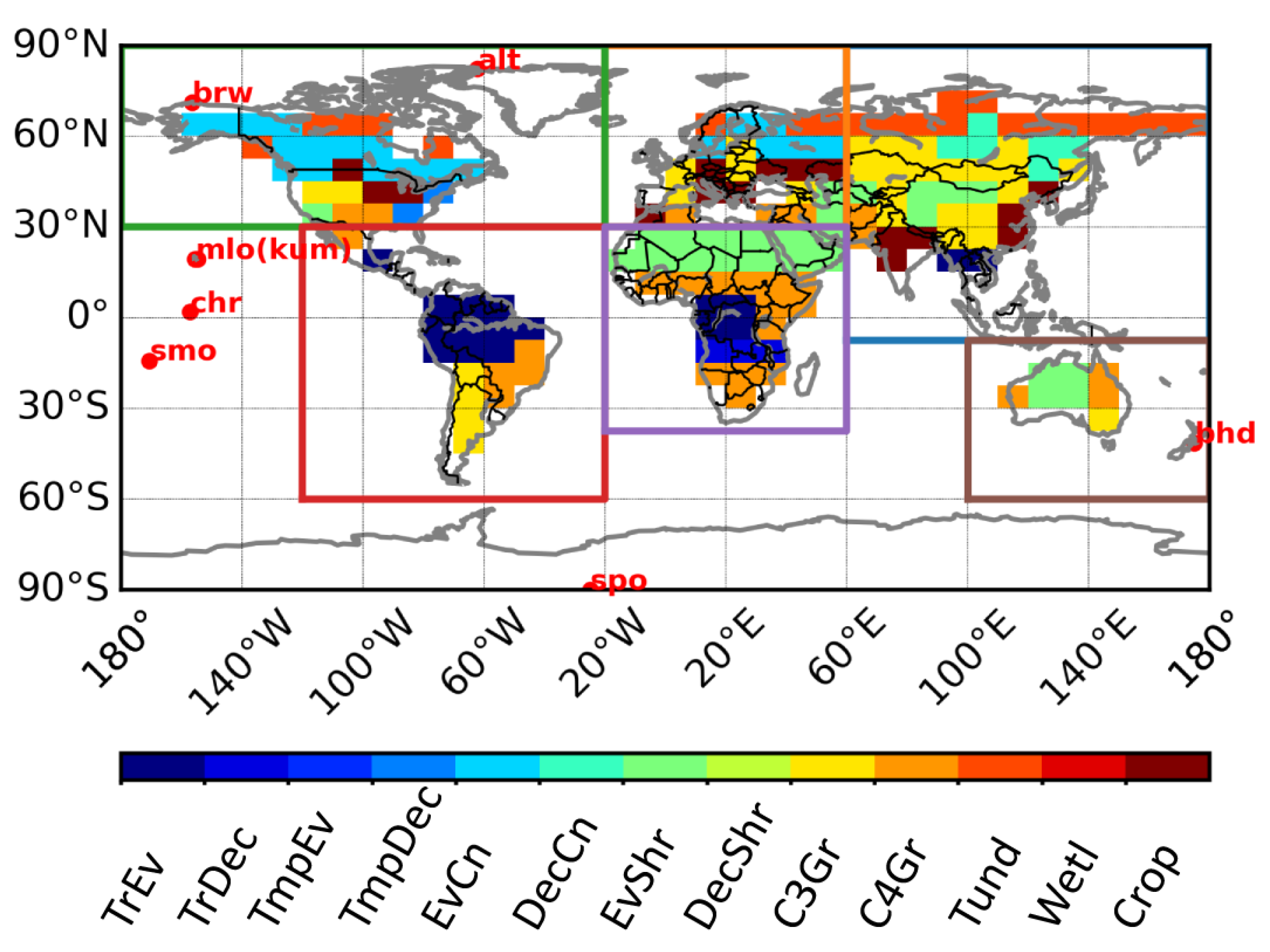
Alert, NWT, Canada	ALT	82.3°N	62.3°W	210
Baring Head, New Zealand	BHD	41.4°S	174.9°E	85
Point Barrow, Alaska	BRW	71.3°N	156.6°W	11
Christmas Island	CHR	2.0°N	157.3°W	2
Cape Kumukahi, Hawaii	KUM	19.5°N	154.8°W	3
Mauna Loa Observatory, Hawaii	MLO	19.5°N	155.6°W	3397
American Samoa	SMO	14.2°S	170.6°W	30
South Pole	SPO	90.0°S		2810

Table A2. CCDAS optimized parameters and their changes in optimization.

No.	Symbol	Description	Units	Prior	Prior unc.	Posterior
1	$V_{c m a x}$	Maximum carboxylation rate (C3/C4) for PFT 1-13: TrEv (1; Tropical broadleaf evergreen tree), TrDec (2; Tropical broadleaf deciduous tree), TmpEv (3; Temperate broadleaf evergreen tree), TmpDec (4; Temperate deciduous tree), EvCn (5; Evergreen coniferous tree), DecCn (6; Deciduous coniferous tree), EvShr (7; Evergreen shrub), DecShr (8; Deciduous)	μmol(CO₂)m-2s-1	6.00 × 10⁻⁵	1.20 × 10⁻⁵	7.84 × 10⁻⁶
2	$V_{c m a x}$		μmol(CO₂)m-2s-1	9.00 × 10⁻⁵	1.80 × 10⁻⁵	2.15 × 10⁻⁴
3	$V_{c m a x}$		μmol(CO₂)m-2s-1	4.10 × 10⁻⁵	8.20 × 10⁻⁶	3.81 × 10⁻⁵
4	$V_{c m a x}$		μmol(CO₂)m-2s-1	3.50 × 10⁻⁵	7.00 × 10⁻⁶	3.46 × 10⁻⁵
5	$V_{c m a x}$		μmol(CO₂)m-2s-1	2.90 × 10⁻⁵	5.80 × 10⁻⁶	4.87 × 10⁻⁵
6	$V_{c m a x}$		μmol(CO₂)m-2s-1	5.30 × 10⁻⁵	1.06 × 10⁻⁵	6.72 × 10⁻⁵
7	$V_{c m a x}$		μmol(CO₂)m-2s-1	5.20 × 10⁻⁵	1.04 × 10⁻⁵	3.49 × 10⁻⁵
8	$V_{c m a x}$		μmol(CO₂)m-2s-1	1.60 × 10⁻⁴	3.20 × 10⁻⁵	9.16 × 10⁻⁵
9	$V_{c m a x}$		μmol(CO₂)m-2s-1	4.20 × 10⁻⁵	8.40 × 10⁻⁶	4.45 × 10⁻⁵
10	$V_{c m a x}$		μmol(CO₂)m-2s-1	8.00 × 10⁻⁶	1.60 × 10⁻⁶	6.54 × 10⁻⁶
11	$V_{c m a x}$		μmol(CO₂)m-2s-1	2.00 × 10⁻⁵	4.00 × 10⁻⁶	2.97 × 10⁻⁷
12	$V_{c m a x}$		μmol(CO₂)m-2s-1	2.00 × 10⁻⁵	4.00 × 10⁻⁶	2.06 × 10⁻⁵
13	$V_{c m a x}$		μmol(CO₂)m-2s-1	1.17 × 10⁻⁴	2.34 × 10⁻⁵	7.07 × 10⁻⁵
14	aJ,V	Ratio Vmax to Jmax (max. electron transport rate) for PFT 1–13	-	1.96	9.80 × 10⁻²	1.81
15	aJ,V		-	1.99	9.95 × 10⁻²	1.75
16	aJ,V		-	2.00	1.00 × 10⁻¹	1.99
17	aJ,V		-	2.00	1.00 × 10⁻¹	2.07
18	aJ,V		-	1.79	8.95 × 10⁻²	1.87
19	aJ,V		-	1.79	8.95 × 10⁻²	1.81
20	aJ,V		-	1.96	9.80 × 10⁻²	1.95
21	aJ,V		-	1.66	8.30 × 10⁻²	1.66
22	aJ,V		-	1.90	9.50 × 10⁻²	1.81
23	aJ,V		-	1.40 × 10⁻⁴	2.80 × 10⁻⁵	4.47 × 10⁻⁵
24	aJ,V		-	1.85	9.25 × 10⁻²	1.80
25	aJ,V		-	1.85	9.25 × 10⁻²	1.84
26	aJ,V		-	1.88	9.40 × 10⁻²	2.13
27	$f_{r, l e a f}$	Leaf respiration ratio	-	4.00 × 10⁻¹	1.00 × 10⁻¹	4.40 × 10⁻¹
28	$f_{r, g r o w t h}$	Growth respiration ratio	-	2.00 × 10⁻¹	1.00 × 10⁻²	2.48 × 10⁻¹
29	$Q_{10, f}$	Soil respiration temperature factor, fast pool	-	1.50	7.50 × 10⁻¹	1.67
30	$Q_{10, s}$	Soil respiration temperature factor, slow pool	-	1.50	7.50 × 10⁻¹	1.35
31	$τ f$	Fast pool soil carbon turnover time	year	6.60 × 10⁻¹	4.00 × 10⁻¹	4.25 × 10⁻²
32	$κ$	Soil moisture exponential for soil respiration	-	1.00	1.00	2.87
33	$f_{S}$	Fraction of fast soil decomposition	-	2.00 × 10⁻¹	2.00 × 10⁻¹	2.32 × 10⁻¹
34	$E_{R d}$	Activation energy, dark respiration	J mol⁻¹	4.50 × 10⁴	2.25 × 10³	2.56 × 10⁴
35	$E_{V m a x}$	Activation energy, carboxylation rate (C₃)	J mol⁻¹	5.85 × 10⁴	2.93 × 10³	6.76 × 10⁴
36	$E_{K O}$	Activation energy, O₂	J mol⁻¹	3.59 × 10⁴	1.80 × 10³	3.58 × 10⁴
37	$E_{K C}$	Activation energy, CO₂	J mol⁻¹	5.94 × 10⁴	2.97 × 10³	5.61 × 10⁴
38	$E_{k}$	Activation energy, carboxylation rate (C₄)	J mol⁻¹	5.10 × 10⁴	2.55 × 10³	5.16 × 10⁴
39	$α_{q}$	Photon capture efficiency (C₃)	-	2.80 × 10⁻¹	1.40 × 10⁻²	2.46 × 10⁻¹
40	$α_{i}$	Quantum efficiency (C₄)	-	4.00 × 10⁻²	2.00 × 10⁻³	3.45 × 10⁻²
41	$K c^{25}$	Michaelis–Menten constant CO₂	μmol(CO₂)mol(air)-1 °C⁻¹	4.60 × 10⁻⁴	2.30 × 10⁻⁵	4.04 × 10⁻⁴
42	$K o^{25}$	Michaelis–Menten constant O₂	μmol(CO₂)mol(air)-1 °C⁻¹	3.30 × 10⁻¹	1.65 × 10⁻²	3.51 × 10⁻¹
43	a $Γ, T$	Temperature slope CO² compensation point	μmol(CO₂)mol(air)-1 °C⁻¹	1.70 × 10⁻⁶	8.50 × 10⁻⁸	1.42 × 10⁻⁶
44	β	Net CO₂ sink/soil factor for PFT 1–13, used for adjusting soil carbon pool3	-	1.00	2.50 × 10⁻¹	4.79 × 10⁻¹
45	β		-	1.00	2.50 × 10⁻¹	1.99
46	β		-	1.00	2.50 × 10⁻¹	1.01
47	β		-	1.00	2.50 × 10⁻¹	3.61 × 10⁻¹
48	β		-	1.00	2.50 × 10⁻¹	2.28 × 10⁻¹
49	β		-	1.00	2.50 × 10⁻¹	7.39 × 10⁻¹
50	β		-	1.00	2.50 × 10⁻¹	1.63
51	β		-	1.00	2.50 × 10⁻¹	1.28
52	β		-	1.00	2.50 × 10⁻¹	1.59
53	β		-	1.00	2.50 × 10⁻¹	1.67
54	β		-	1.00	2.50 × 10⁻¹	6.32 × 10⁻¹
55	β		-	1.00	2.50 × 10⁻¹	9.36 × 10⁻¹
56	β		-	1.00	2.50 × 10⁻¹	6.55 × 10⁻²
57	$Λ ~$	Maximum leaf area index	-	4.00	1.00 × 10⁻¹	3.41
58	$T_{ϕ}$	Phenology temperature trigger for PFT 4–6	°C	1.00 × 10¹	2.00	6.99
59	$T_{ϕ}$	Phenology temperature trigger for PFT 8	°C	8.00	2.00	8.26
60	$T_{ϕ}$	Phenology temperature trigger for PFT 9–12	°C	2.00	2.00	-2.20
61	$T_{ϕ}$	Phenology temperature trigger for PFT 13	°C	1.50 × 10¹	2.00	2.32 × 10¹
62	$T_{r}$	Spatial range of phenology temperature trigger for PFT 4–6, 8, 13	°C	2.00	1.00	2.06
63	$T_{r}$	Spatial range of phenology temperature trigger for PFT 9–12	°C	2.00	1.00	1.74 × 10⁻¹
64	$t_{c}$	Day length at leaf shedding for PFT 4–6, 8, 11	hour	1.05 × 10¹	1.00	5.40
65	$t_{r}$	Spatial range of day length at leaf shedding for PFT 4–6, 8, 11	hour	5.00 × 10⁻¹	2.50 × 10⁻¹	7.78 × 10⁻¹
66	$ξ$	Initial linear leaf growth	d⁻¹	5.00 × 10⁻¹	5.00 × 10⁻¹	8.44 × 10⁻¹
67	$k_{L}$	Inverse of leaf longevity for PFT 2, 4, 6, 8–10, 12, 13	hour	1.00 × 10⁻¹	1.00 × 10⁻¹	4.72 × 10⁻³
68	$k_{L}$	Inverse of leaf longevity for PFT 5, 11	hour	5.00 × 10⁻³	5.00 × 10⁻³	1.11 × 10⁻²
69	$τ w$	Length of dry spell before leaf shedding for PFT 1, 3, 7	d⁻¹	3.00 × 10¹	3.00 × 10¹	4.46 × 10¹
70	$τ w$	Length of dry spell before leaf shedding for PFT 2	d⁻¹	3.00 × 10¹	3.00 × 10¹	9.66
71	$τ w$	Length of dry spell before leaf shedding for PFT 9–10, 12, 13	day	3.00 × 10¹	3.00 × 10¹	8.10
72	$f C_{i}, C_{3}$	Stomata internal to atmospheric CO₂ (C3)	-	6.50 × 10⁻¹	6.50 × 10⁻²	5.55 × 10⁻¹
73	$f C_{i}, C_{4}$	Stomata internal to atmospheric CO₂ (C4)	-	3.70 × 10⁻¹	3.70 × 10⁻²	4.47 × 10⁻¹
74	$C_{W 0}$	Ratio of maximum water supply rate	mm d⁻¹	5.00 × 10⁻¹	1.50 × 10⁻¹	9.56 × 10⁻¹
75	emis0	Emissivity of the atmosphere	-	6.40 × 10⁻¹	3.20 × 10⁻²	7.51 × 10⁻¹
76	srdepth	Rooting depth scalar for PFT 1–13	-	1.00	1.00 × 10⁻¹	9.47 × 10⁻¹
77	srdepth		-	1.00	1.00 × 10⁻¹	4.59 × 10⁻¹
78	srdepth		-	1.00	1.00 × 10⁻¹	9.91 × 10⁻¹
79	srdepth		-	1.00	1.00 × 10⁻¹	9.77 × 10⁻¹
80	srdepth		-	1.00	1.00 × 10⁻¹	1.12
81	srdepth		-	1.00	1.00 × 10⁻¹	9.02 × 10⁻¹
82	srdepth		-	1.00	1.00 × 10⁻¹	1.07
83	srdepth		-	1.00	1.00 × 10⁻¹	1.20
84	srdepth		-	1.00	1.00 × 10⁻¹	6.14 × 10⁻¹
85	srdepth		-	1.00	1.00 × 10⁻¹	4.40 × 10⁻¹
86	srdepth		-	1.00	1.00 × 10⁻¹	1.02
87	srdepth		-	1.00	1.00 × 10⁻¹	9.90 × 10⁻¹
88	srdepth		-	1.00	1.00 × 10⁻¹	1.47
89	Sb	Shape parameter retention curve scalar for soil texture 1-6: coarse (1; loam sand), medium/coarse (2; sandy loam), medium (3; loam), fine/medium (4; sandy clay loam), fine (5; clay loam), organic (6; loam)	-	1.00	1.00 × 10⁻¹	8.18 × 10⁻¹
90	Sb		-	1.00	1.00 × 10⁻¹	8.89 × 10⁻¹
91	Sb		-	1.00	1.00 × 10⁻¹	1.20
92	Sb		-	1.00	1.00 × 10⁻¹	1.16
93	Sb		-	1.00	1.00 × 10⁻¹	7.19 × 10⁻¹
94	Sb		-	1.00	1.00 × 10⁻¹	9.91 × 10⁻¹
95	Sn	Soil porosity scalar for soil texture 1-6	-	1.00	1.00 × 10⁻¹	1.33
96	Sn		-	1.00	1.00 × 10⁻¹	3.15 × 10⁻¹
97	Sn		-	1.00	1.00 × 10⁻¹	1.04
98	Sn		-	1.00	1.00 × 10⁻¹	6.26 × 10⁻¹
99	Sn		-	1.00	1.00 × 10⁻¹	1.30
100	Sn		-	1.00	1.00 × 10⁻¹	9.91 × 10⁻¹
101	Offset	Initial atmospheric CO₂ concentration	ppm	3.36 × 10²	1.00	3.37 × 10²

These 101 parameters are related to physiology (parameters 1 to 57), phenology (58 to 71), stomatal control (72 to 74), energy balance (75), soil hydrology (76-100), and atmospheric CO2 concentration (101). More details see Wu et al., 2020.

Figure A1. Comparison of prior and optimized output of CO₂ concentrations at eight sites with SIO data. (a) is ALT site, (b) is BHD site, (c) is BRW site, (d) is CHR site, (e) is KUM site, (f) is MLO site, (g) is SMO site, and (h) is SPO site. The “prior”, “co₂”, and “sm + co₂” experiments are represented by blue, orange, and green lines, respectively; the SIO observations are represented by black dot. Simulation results and observations are depicted with monthly data, The RMSEs for these three experiments are represented by the values in the legend, in ppm.

Figure A2. Time series anomalies of soil moisture from ESA-CCI and from CCDAS optimization (‘sm+co₂’) at various latitudes. (a–e) denotes different latitude. The anomalies are calculated from the mean surface soil moisture for each latitudinal band. Red lines for CCI and blue lines for CCDAS (‘sm+co₂’). The correlations of soil moisture anomalies and two ENSO indices (MEI and Niño 3.4) are depicted in each figure.

Figure A3. Inter-annual variability of ENSO indices, soil water, NEP, and CO₂ concentrations. (a), normalized anomalies for two ENSO indices, MEI (Multivariate ENSO Index) and Niño 3.4, anomalies are calculated by removing mean seasonality during 1980–2015, then normalized by standard deviations for the same period. (b), soil moisture anomalies calculated from zonal mean soil moisture (30°N-60°N) by removing mean seasonality during 1980–2015 and then smoothed with a 7-month moving average method, for both the CCI remote sensing data and CCDAS-optimized soil moisture. (c), NEP anomalies calculated from global mean CCDAS-optimized NEP using the same method as soil moisture. (d), global CO₂ growth rate (CGR) anomalies calculated from the global CO₂ concentrations by mixing CO₂ concentrations from Mauna Loa (MLO) and South Pole (SPO), 0.75 × MLO + 0.25 × SPO, and deriving the growth rate by removing mean seasonality, then a 7-month moving average is used for SIO CO₂ concentrations and CCDAS-optimized CO₂ concentrations, respectively. (e), GPP anomalies calculated from global mean CCDAS-optimized GPP using the same method as soil moisture. Correlation coefficients (Pearson r) are derived from the best values at different time lags between different variables and strong El Niño/La Niña events (values from the colored region in Figure 1a).

Figure A4. Relations between Pearson r and time lag. (a), changes in Pearson r for CCI soil moisture and CCDAS-optimized soil moisture with time lag response of soil moisture to two ENSO indices, MEI and Niño 3.4. (b), same as (a), but for atmospheric inversion from Jena CarboScope and CCDAS-optimized NEP. (c), same as (a), but for global CO₂ growth rate (CGR) from SIO and CCDAS optimization.

Figure A5. Time series anomalies of GPP from FLUXCOM and from CCDAS optimization (‘sm+co₂’) at various latitudes. (a–e) denote different latitudes. The anomalies are calculated from the mean GPP for each latitudinal band. Red lines for FLUXCOM and blue lines for CCDAS (‘sm+co₂’). The correlations of GPP anomalies and two ENSO indices (MEI and Niño 3.4) are depicted in each figure.

Figure A6. The power spectra of simulated GPP and NEP (by column) with different experiments (by color) in different latitude bands (by row). The mean seasonal cycle of all monthly variables is removed. GPP for gross primary productivity, NEP for net ecosystem productivity. Blue color denotes results from the prior model simulation with prescribed parameter values, black color denotes the atmospheric CO₂ only assimilation results, and red color denotes the results from the simultaneous assimilation of soil moisture and atmospheric CO₂. The colored digits in each panel denote the Pearson r of spectra pattern between soil moisture (3rd column) and other variables (1st and 2nd columns) from different simulation experiments.

Figure A7. Global vegetation map and continental boundaries as well as atmospheric CO₂ observation stations. A total of 13 PFTs are defined in CCDAS and the major PFT for each grid cell is shown here. The continental boundaries are depicted with rectangles, green color for North America, red color for South America, yellow color for Europe, purple color for South Africa, blue color for Asia, and brown color for Oceania. The red dots are for the SIO atmospheric CO₂ observation stations from which the data are used in the assimilation.

Figure A8. Relations between Pearson r and time lag. (a), changes in Pearson r for CCDAS-optimized soil moisture with time-lag response of continental soil moisture to two ENSO indices, MEI and Niño 3.4. (b), same as (a), but for NEP. (c), same as (a), but for GPP.

References

Allen, C.D.; Breshears, D.D.; McDowell, N.G. On underestimation of global vulnerability to tree mortality and forest die-off from hotter drought in the Anthropocene. Ecosphere 2015, 6, 1–55. [Google Scholar] [CrossRef]
Beer, C.; Reichstein, M.; Tomelleri, E.; Ciais, P.; Jung, M.; Carvalhais, N.; Rodenbeck, C.; Arain, M.A.; Baldocchi, D.; Bonan, G.B.; et al. Terrestrial gross carbon dioxide uptake: Global distribution and covariation with climate. Science 2010, 329, 834–838. [Google Scholar] [CrossRef] [PubMed] [Green Version]
Braswell, B.H.; Schimel, D.S.; Linder, E.; Moore, B. The response of global terrestrial ecosystems to interannual temperature variability. Science 1997, 278, 870–873. [Google Scholar] [CrossRef]
Potter, C.; Klooster, S.; Steinbach, M.; Tan, P.; Kumar, V.; Shekhar, S.; Nemani, R.; Myneni, R. Global teleconnections of climate to terrestrial carbon flux. J. Geophys. Res. 2003, 108, 4556. [Google Scholar] [CrossRef] [Green Version]
Keeling, C.D.; Whorf, T.P.; Wahlen, M.; Van der Plichtt, J. Interannual extremes in the rate of rise of atmospheric carbon dioxide since 1980. Nature 1995, 375, 666–670. [Google Scholar] [CrossRef]
Zhu, Z.; Piao, S.; Xu, Y.; Bastos, A.; Ciais, P.; Peng, S. The effects of teleconnections on carbon fluxes of global terrestrial ecosystems. Geophys. Res. Lett. 2017, 44, 3209–3218. [Google Scholar] [CrossRef]
Wang, S.; Zhang, Y.; Ju, W.; Qiu, B.; Zhang, Z. Tracking the seasonal and inter-annual variations of global gross primary production during last four decades using satellite near-infrared reflectance data. Sci. Total Environ. 2021, 755, 142569. [Google Scholar] [CrossRef]
Cai, W.; Yuan, W.; Liang, S.; Liu, S.; Dong, W.; Chen, Y.; Liu, D.; Zhang, H. Large Differences in Terrestrial Vegetation Production Derived from Satellite-Based Light Use Efficiency Models. Remote Sens. 2014, 6, 8945–8965. [Google Scholar] [CrossRef] [Green Version]
Anav, A.; Friedlingstein, P.; Beer, C.; Ciais, P.; Harper, A.; Jones, C.; Murray-Tortarolo, G.; Papale, D.; Parazoo, N.C.; Peylin, P.; et al. Spatiotemporal patterns of terrestrial gross primary production: A review. Rev. Geophys. 2015, 53, 785–818. [Google Scholar] [CrossRef] [Green Version]
Rayner, P.J.; Law, R.M. The interannual variability of the global carbon cycle. Tellus B Chem. Phys. Meteorol. 2016, 51, 210–212. [Google Scholar] [CrossRef]
Frankenberg, C.; Fisher, J.B.; Worden, J.; Badgley, G.; Saatchi, S.S.; Lee, J.-E.; Toon, G.C.; Butz, A.; Jung, M.; Kuze, A.; et al. New global observations of the terrestrial carbon cycle from GOSAT: Patterns of plant fluorescence with gross primary productivity. Geophys. Res. Lett. 2011, 38, L17706. [Google Scholar] [CrossRef] [Green Version]
Yuan, W.; Liu, S.; Yu, G.; Bonnefond, J.-M.; Chen, J.; Davis, K.; Desai, A.R.; Goldstein, A.H.; Gianelle, D.; Rossi, F.; et al. Global estimates of evapotranspiration and gross primary production based on MODIS and global meteorology data. Remote Sens. Environ. 2010, 114, 1416–1431. [Google Scholar] [CrossRef] [Green Version]
Ma, N.; Niu, G.-Y.; Xia, Y.; Cai, X.; Zhang, Y.; Ma, Y.; Fang, Y. A Systematic Evaluation of Noah-MP in Simulating Land-Atmosphere Energy, Water, and Carbon Exchanges Over the Continental United States. J. Geophys. Res. Atmos. 2017, 122, 12, 245–212, 268. [Google Scholar] [CrossRef] [Green Version]
Piao, S.; Sitch, S.; Ciais, P.; Friedlingstein, P.; Peylin, P.; Wang, X.; Ahlstrom, A.; Anav, A.; Canadell, J.G.; Cong, N.; et al. Evaluation of terrestrial carbon cycle models for their response to climate variability and to CO₂ trends. Globle Chang. Biol. 2013, 19, 2117–2132. [Google Scholar] [CrossRef] [Green Version]
Jung, M.; Reichstein, M.; Schwalm, C.R.; Huntingford, C.; Sitch, S.; Ahlström, A.; Arneth, A.; Camps-Valls, G.; Ciais, P.; Friedlingstein, P.; et al. Compensatory water effects link yearly global land CO₂ sink changes to temperature. Nature 2017, 541, 516–520. [Google Scholar] [CrossRef] [Green Version]
Sitch, S.; Friedlingstein, P.; Gruber, N.; Jones, S.D.; Murray-Tortarolo, G.; Ahlström, A.; Doney, S.C.; Graven, H.; Heinze, C.; Huntingford, C.; et al. Recent trends and drivers of regional sources and sinks of carbon dioxide. Biogeosciences 2015, 12, 653–679. [Google Scholar] [CrossRef] [Green Version]
Keenan, T.F.; Baker, I.; Barr, A.; Ciais, P.; Davis, K.; Dietze, M.; Dragoni, D.; Gough, C.M.; Grant, R.; Hollinger, D.; et al. Terrestrial biosphere model performance for inter-annual variability of land-atmosphere CO₂ exchange. Glob. Chang. Biol. 2012, 18, 1971–1987. [Google Scholar] [CrossRef]
Schaefer, K.; Schwalm, C.R.; Williams, C.; Arain, M.A.; Barr, A.; Chen, J.M.; Davis, K.J.; Dimitrov, D.; Hilton, T.W.; Hollinger, D.Y.; et al. A model-data comparison of gross primary productivity: Results from the North American Carbon Program site synthesis. J. Geophys. Res. Biogeosci. 2012, 117, G03010. [Google Scholar] [CrossRef] [Green Version]
Rayner, P.J.; Scholze, M.; Knorr, W.; Kaminski, T.; Giering, R.; Widmann, H. Two decades of terrestrial carbon fluxes from a carbon cycle data assimilation system (CCDAS). Glob. Biogeochem. Cycles 2005, 19, GB2026. [Google Scholar] [CrossRef] [Green Version]
Knorr, W.; Kaminski, T.; Scholze, M.; Gobron, N.; Pinty, B.; Giering, R.; Mathieu, P.-P. Carbon cycle data assimilation with a generic phenology model. J. Geophys. Res. Biogeosci. 2010, 115, G04017. [Google Scholar] [CrossRef]
Kaminski, T.; Knorr, W.; Scholze, M.; Gobron, N.; Pinty, B.; Giering, R.; Mathieu, P.P. Consistent assimilation of MERIS FAPAR and atmospheric CO₂ into a terrestrial vegetation model and interactive mission benefit analysis. Biogeosciences 2012, 9, 3173–3184. [Google Scholar] [CrossRef] [Green Version]
Scholze, M.; Kaminski, T.; Knorr, W.; Blessing, S.; Vossbeck, M.; Grant, J.P.; Scipal, K. Simultaneous assimilation of SMOS soil moisture and atmospheric CO₂ in-situ observations to constrain the global terrestrial carbon cycle. Remote Sens. Environ. 2016, 180, 334–345. [Google Scholar] [CrossRef]
Wu, M.; Scholze, M.; Kaminski, T.; Voßbeck, M.; Tagesson, T. Using SMOS soil moisture data combining CO₂ flask samples to constrain carbon fluxes during 2010–2015 within a Carbon Cycle Data Assimilation System (CCDAS). Remote Sens. Environ. 2020, 240, 111719. [Google Scholar] [CrossRef]
Zhao, M.; Running, S.W. Drought-induced reduction in global terrestrial net primary production from 2000 through 2009. Science 2010, 329, 940–943. [Google Scholar] [CrossRef] [PubMed] [Green Version]
Piao, S.; Zhang, X.; Chen, A.; Liu, Q.; Lian, X.; Wang, X.; Peng, S.; Wu, X. The impacts of climate extremes on the terrestrial carbon cycle: A review. Sci. China Earth Sci. 2019, 62, 1551–1563. [Google Scholar] [CrossRef]
Wu, X.; Liu, H.; Li, X.; Ciais, P.; Babst, F.; Guo, W.; Zhang, C.; Magliulo, V.; Pavelka, M.; Liu, S.; et al. Differentiating drought legacy effects on vegetation growth over the temperate Northern Hemisphere. Glob. Chang. Biol. 2018, 24, 504–516. [Google Scholar] [CrossRef]
Allen, C.D.; Macalady, A.K.; Chenchouni, H.; Bachelet, D.; McDowell, N.; Vennetier, M.; Kitzberger, T.; Rigling, A.; Breshears, D.D.; Hogg, E.H.; et al. A global overview of drought and heat-induced tree mortality reveals emerging climate change risks for forests. For. Ecol. Manag. 2010, 259, 660–684. [Google Scholar] [CrossRef] [Green Version]
Brienen, R.J.; Phillips, O.L.; Feldpausch, T.R.; Gloor, E.; Baker, T.R.; Lloyd, J.; Lopez-Gonzalez, G.; Monteagudo-Mendoza, A.; Malhi, Y.; Lewis, S.L.; et al. Long-term decline of the Amazon carbon sink. Nature 2015, 519, 344–348. [Google Scholar] [CrossRef] [Green Version]
Trugman, A.T.; Medvigy, D.; Anderegg, W.R.L.; Pacala, S.W. Differential declines in Alaskan boreal forest vitality related to climate and competition. Glob. Chang. Biol. 2018, 24, 1097–1107. [Google Scholar] [CrossRef] [Green Version]
Orth, R.; Destouni, G.; Jung, M.; Reichstein, M. Large-scale biospheric drought response intensifies linearly with drought duration in arid regions. Biogeosciences 2020, 17, 2647–2656. [Google Scholar] [CrossRef]
Stocker, B.D.; Zscheischler, J.; Keenan, T.F.; Prentice, I.C.; Seneviratne, S.I.; Peñuelas, J. Drought impacts on terrestrial primary production underestimated by satellite monitoring. Nat. Geosci. 2019, 12, 264–270. [Google Scholar] [CrossRef] [Green Version]
Schewe, J.; Gosling, S.N.; Reyer, C.; Zhao, F.; Ciais, P.; Elliott, J.; Francois, L.; Huber, V.; Lotze, H.K.; Seneviratne, S.I.; et al. State-of-the-art global models underestimate impacts from climate extremes. Nat. Commun. 2019, 10, 1005. [Google Scholar] [CrossRef] [Green Version]
Trugman, A.T.; Medvigy, D.; Mankin, J.S.; Anderegg, W.R.L. Soil moisture stress as a major driver of carbon cycle uncertainty. Geophysical Research Letters. 2018, 45, 6495–6503. [Google Scholar] [CrossRef]
Friend, A.D.; Lucht, W.; Rademacher, T.T.; Keribin, R.; Betts, R.; Cadule, P.; Ciais, P.; Clark, D.B.; Dankers, R.; Falloon, P.D.; et al. Carbon residence time dominates uncertainty in terrestrial vegetation responses to future climate and atmospheric CO₂. Proc. Natl. Acad. Sci. USA 2014, 111, 3280–3285. [Google Scholar] [CrossRef] [Green Version]
Friedlingstein, P.; Meinshausen, M.; Arora, V.K.; Jones, C.D.; Anav, A.; Liddicoat, S.K.; Knutti, R. Uncertainties in CMIP5 Climate Projections due to Carbon Cycle Feedbacks. J. Clim. 2014, 27, 511–526. [Google Scholar] [CrossRef] [Green Version]
Green, J.K.; Seneviratne, S.I.; Berg, A.M.; Findell, K.L.; Hagemann, S.; Lawrence, D.M.; Gentine, P. Large influence of soil moisture on long-term terrestrial carbon uptake. Nature 2019, 565, 476–479. [Google Scholar] [CrossRef]
Humphrey, V.; Zscheischler, J.; Ciais, P.; Gudmundsson, L.; Sitch, S.; Seneviratne, S.I. Sensitivity of atmospheric CO₂ growth rate to observed changes in terrestrial water storage. Nature 2018, 560, 628–631. [Google Scholar] [CrossRef]
Peters, W.; van der Velde, I.R.; van Schaik, E.; Miller, J.B.; Ciais, P.; Duarte, H.F.; van der Laan-Luijkx, I.T.; van der Molen, M.K.; Scholze, M.; Schaefer, K.; et al. Increased water-use efficiency and reduced CO₂ uptake by plants during droughts at a continental-scale. Nat. Geosci. 2018, 11, 744–748. [Google Scholar] [CrossRef] [Green Version]
Trenberth, K.E.; Dai, A.; van der Schrier, G.; Jones, P.D.; Barichivich, J.; Briffa, K.R.; Sheffield, J. Global warming and changes in drought. Nat. Clim. Chang. 2013, 4, 17–22. [Google Scholar] [CrossRef]
Zhou, S.; Zhang, Y.; Williams, A.P.; Gentine, P. Projected increases in intensity, frequency, and terrestrial carbon costs of compound drought and aridity events. Sci. Adv. 2019, 5, eaau5740. [Google Scholar] [CrossRef]
Liu, L.; Gudmundsson, L.; Hauser, M.; Qin, D.; Li, S.; Seneviratne, S.I. Soil moisture dominates dryness stress on ecosystem production globally. Nat Commun 2020, 11, 4892. [Google Scholar] [CrossRef] [PubMed]
Barbu, A.L.; Calvet, J.C.; Mahfouf, J.F.; Lafont, S. Integrating ASCAT surface soil moisture and GEOV1 leaf area index into the SURFEX modelling platform: A land data assimilation application over France. Hydrol. Earth Syst. Sci. 2014, 18, 173–192. [Google Scholar] [CrossRef] [Green Version]
van der Molen, M.K.; de Jeu, R.A.M.; Wagner, W.; van der Velde, I.R.; Kolari, P.; Kurbatova, J.; Varlagin, A.; Maximov, T.C.; Kononov, A.V.; Ohta, T.; et al. The effect of assimilating satellite-derived soil moisture data in SiBCASA on simulated carbon fluxes in Boreal Eurasia. Hydrol. Earth Syst. Sci. 2016, 20, 605–624. [Google Scholar] [CrossRef] [Green Version]
Seneviratne, S.I.; Corti, T.; Davin, E.L.; Hirschi, M.; Jaeger, E.B.; Lehner, I.; Orlowsky, B.; Teuling, A.J. Investigating soil moisture–climate interactions in a changing climate: A review. Earth Sci. Rev. 2010, 99, 125–161. [Google Scholar] [CrossRef]
He, L.; Chen, J.M.; Liu, J.; Mo, G.; Bélair, S.; Zheng, T.; Wang, R.; Chen, B.; Croft, H.; Arain, M.A.; et al. Optimization of water uptake and photosynthetic parameters in an ecosystem model using tower flux data. Ecol. Model. 2014, 294, 94–104. [Google Scholar] [CrossRef]
Mu, Q.; Zhao, M.; Heinsch, F.A.; Liu, M.; Tian, H.; Running, S.W. Evaluating water stress controls on primary production in biogeochemical and remote sensing based models. J. Geophys. Res. 2007, 112, G01012. [Google Scholar] [CrossRef] [Green Version]
Bonan, G.B.; Williams, M.; Fisher, R.A.; Oleson, K.W. Modeling stomatal conductance in the earth system: Linking leaf water-use efficiency and water transport along the soil–plant–atmosphere continuum. Geosci. Model Dev. 2014, 7, 2193–2222. [Google Scholar] [CrossRef] [Green Version]
Han, X.; Franssen, H.-J.H.; Montzka, C.; Vereecken, H. Soil moisture and soil properties estimation in the Community Land Model with synthetic brightness temperature observations. Water Resour. Res. 2014, 50, 6081–6105. [Google Scholar] [CrossRef] [Green Version]
Wanders, N.; Karssenberg, D.; de Roo, A.; de Jong, S.M.; Bierkens, M.F.P. The suitability of remotely sensed soil moisture for improving operational flood forecasting. Hydrol. Earth Syst. Sci. 2014, 18, 2343–2357. [Google Scholar] [CrossRef] [Green Version]
Knorr, W. Annual and interannual CO₂ exchanges of the terrestrial biosphere: Process-based simulations and uncertainties. Glob. Ecol. Biogeogr. 2000, 9, 225–252. [Google Scholar] [CrossRef]
Heimann, M. The Global Atmospheric Tracer Model TM2; Technical Report no. 10; Max-Planck-Institut für Meteorologie: Hamburg, Germany, 1995. [Google Scholar]
Marland, G.; Boden, T.A.; Andres, R.J. Global, regional, and national CO₂ emission estimates from fossil fuel burning, cement production, and gas flaring: 1751-1999. Carbon Dioxide Inf. Anal. Cent. 2022. [Google Scholar]
Friedlingstein, P.; O’Sullivan, M.; Jones, M.W.; Andrew, R.M.; Hauck, J.; Olsen, A.; Peters, G.P.; Peters, W.; Pongratz, J.; Sitch, S.; et al. Global Carbon Budget 2020. Earth Syst. Sci. Data 2020, 12, 3269–3340. [Google Scholar] [CrossRef]
Takahashi, T.; Wanninkhof, W.H.; Feely, R.A.; Weiss, R.F.; Chipman, D.W.; Bates, N.R.; Olafsson, J.; Sabine, C.L.; Sutherland, S.G. Net sea-air CO₂ flux over the global oceans: An improved estimate based on the sea-air pCO2 difference. In Proceedings of the Second International Symposium, CO₂ in the Oceans, Tsukuba, Japan, 18–22 January 1999; Nojiri, Y., Ed.; Center for Global Environmental Research, National Institute for Environmental Studies, Environmental Agency of Japan: Tsukuba, Japan, 1999; pp. 9–14. [Google Scholar]
Heimann, M.; Körner, S. The Global Atmospheric Tracer Model TM3: Model Description and User’s Manual Release 3.8a; Technical Report no. 5; Max-Planck-Institute for Biogeochemistry: Jena, Germany, 2003. [Google Scholar]
Houghton, R.A.; Boone, R.D.; Fruci, J.R.; Hobbie, J.E.; Melillo, J.M.; Palm, C.A.; Peterson, B.J.; Shaver, G.R.; Woodwell, G.M.; Moore, B.; et al. The flux of carbon from terrestrial ecosystems to the atmosphere in 1980 due to changes in land use: Geographic distribution of the global flux. Tellus B Chem. Phys. Meteorol. 1987, 39, 122–139. [Google Scholar] [CrossRef]
Fletcher, R.; Powell, M.J.D. A rapidly convergent descent method for minimization. Comput. J. 1963, 6, 163–168. [Google Scholar] [CrossRef] [Green Version]
Viovy, N. CRUNCEP Version 7—Atmospheric forcing data for the community land model. Research Data Archive at the National Center for Atmospheric Research, Computational and Information Systems Laboratory. 2018. Available online: http://rda.ucar.edu/datasets/ds314.3/. (accessed on 22 February 2022).
Keeling, C.D.; Piper, S.C.; Bacastow, R.B.; Wahlen, M.; Whorf, T.P.; Heimann, M.; Meijer, H.A. Exchanges of Atmospheric CO₂ and 13CO₂ with the Terrestrial Biosphere and Oceans from 1978 to 2000. I. Global Aspects. UC San Diego: Scripps Institution of Oceanography. 2001. Retrieved from. Available online: https://escholarship.org/uc/item/09v319r9 (accessed on 18 November 2021).
Gruber, A.; Scanlon, T.; van der Schalie, R.; Wagner, W.; Dorigo, W. Evolution of the ESA CCI Soil Moisture climate data records and their underlying merging methodology. Earth Syst. Sci. Data 2019, 11, 717–739. [Google Scholar] [CrossRef] [Green Version]
Dorigo, W.; Wagner, W.; Albergel, C.; Albrecht, F.; Balsamo, G.; Brocca, L.; Chung, D.; Ertl, M.; Forkel, M.; Gruber, A.; et al. ESA CCI Soil Moisture for improved Earth system understanding: State-of-the art and future directions. Remote Sens. Environ. 2017, 203, 185–215. [Google Scholar] [CrossRef]
Humphrey, V.; Gudmundsson, L. GRACE-REC: A reconstruction of climate-driven water storage changes over the last century. Earth Syst. Sci. Data 2019, 11, 1153–1170. [Google Scholar] [CrossRef] [Green Version]
Rödenbeck, C. Estimating CO₂ Sources and Sinks from Atmospheric Mixing Ratio Measurements using a Global Inversion of Atmospheric Transport; Technical Report no. 6; Max-Planck-Institute for Biogeochemistry: Jena, Germany, 2005. [Google Scholar]
Rödenbeck, C.; Houweling, S.; Gloor, M.; Heimann, M. CO₂ flux history 1982–2001 inferred from atmospheric data using a global inversion of atmospheric transport. Atmos. Chem. Phys. 2003, 3, 1919–1964. [Google Scholar] [CrossRef] [Green Version]
Pastorello, G.; Trotta, C.; Canfora, E.; Chu, H.; Christianson, D.; Cheah, Y.W.; Poindexter, C.; Chen, J.; Elbashandy, A.; Humphrey, M.; et al. The FLUXNET2015 dataset and the ONEFlux processing pipeline for eddy covariance data. Sci. Data 2020, 7, 225. [Google Scholar] [CrossRef]
Vicente-Serrano, S.M.; Beguería, S.; López-Moreno, J.I. A Multiscalar Drought Index Sensitive to Global Warming: The Standardized Precipitation Evapotranspiration Index. J. Clim. 2010, 23, 1696–1718. [Google Scholar] [CrossRef] [Green Version]
Le Quéré, C.; Andrew, R.M.; Friedlingstein, P.; Sitch, S.; Hauck, J.; Pongratz, J.; Pickers, P.A.; Korsbakken, J.I.; Peters, G.P.; Canadell, J.G.; et al. Global Carbon Budget 2018. Earth Syst. Sci. Data 2018, 10, 2141–2194. [Google Scholar] [CrossRef]
Pinzon, J.; Tucker, C. A Non-Stationary 1981–2012 AVHRR NDVI3g Time Series. Remote Sens. 2014, 6, 6929–6960. [Google Scholar] [CrossRef] [Green Version]
Tucker, C.J.; Pinzon, J.E.; Brown, M.E.; Slayback, D.A.; Pak, E.W.; Mahoney, R.; Vermote, E.F.; El Saleous, N. An extended AVHRR 8-km NDVI dataset compatible with MODIS and SPOT vegetation NDVI data. Int. J. Remote Sens. 2010, 26, 4485–4498. [Google Scholar] [CrossRef]
Wang, S.; Zhang, Y.; Ju, W.; Wu, M.; Liu, L.; He, W.; Peñuelas, J. Temporally corrected long-term satellite solar-induced fluorescence leads to improved estimation of global trends in vegetation photosynthesis during 1995–2018. ISPRS J. Photogramm. Remote Sens. 2022, 194, 222–234. [Google Scholar] [CrossRef]
Wolter, K.; Timlin, M.S. El Niño/Southern Oscillation behaviour since 1871 as diagnosed in an extended multivariate ENSO index (MEI.ext). Int. J. Climatol. 2011, 31, 1074–1087. [Google Scholar] [CrossRef]
Wolter, K.; Timlin, M.S. Measuring the strength of ENSO events: How does 1997/98 rank? Weather 1998, 53, 315–324. [Google Scholar] [CrossRef]
Wolter, K.; Timlin, M.S. Monitoring ENSO in COADS with a seasonally adjusted principal component index. In Proceedings of the 17th Climate Diagnostics Workshop, Norman, OK, USA, 18–23 October 1992. [Google Scholar]
Rayner, N.A.; Parker, D.E.; Horton, E.B.; Folland, C.K.; Alexander, L.V.; Rowell, D.P.; Kent, E.C.; Kaplan, A. Global analyses of sea surface temperature, sea ice, and night marine air temperature since the late nineteenth century. J. Geophys. Res. 2003, 108, 4407. [Google Scholar] [CrossRef] [Green Version]
Frigo, M.; Johnson, S.G. FFTW: An Adaptive Software Architecture for the FFT . Proc. Int. Conf. Acoust. Speech Signal Process. 1998, 3, 1381–1384. [Google Scholar]
Dai, A.; Qian, T.; Trenberth, K.E.; Millliman, J.D. Changes in Continental Freshwater Discharge from 1948 to 2004. J. Clim. 2009, 22, 2773–2792. [Google Scholar] [CrossRef]
Miralles, D.G.; van den Berg, M.J.; Gash, J.H.; Parinussa, R.M.; de Jeu, R.A.M.; Beck, H.E.; Holmes, T.R.H.; Jiménez, C.; Verhoest, N.E.C.; Dorigo, W.A.; et al. El Niño–La Niña cycle and recent trends in continental evaporation. Nat. Clim. Chang. 2013, 4, 122–126. [Google Scholar] [CrossRef]
Patra, P.K.; Maksyutov, S.; Nakazawa, T. Analysis of atmospheric CO₂ growth rates at Mauna Loa using CO₂ fluxes derived from an inverse model. Tellus B Chem. Phys. Meteorol. 2017, 57, 357–365. [Google Scholar] [CrossRef]
Gonsamo, A.; Chen, J.M.; Lombardozzi, D. Global vegetation productivity response to climatic oscillations during the satellite era. Glob. Chang. Biol. 2016, 22, 3414–3426. [Google Scholar] [CrossRef]
Zhang, Y.; Dannenberg, M.P.; Hwang, T.; Song, C. El Niño-Southern Oscillation-Induced Variability of Terrestrial Gross Primary Production During the Satellite Era. J. Geophys. Res. Biogeosci. 2019, 124, 2419–2431. [Google Scholar] [CrossRef]
Vicente-Serrano, S.M.; López-Moreno, J.I.; Gimeno, L.; Nieto, R.; Morán-Tejeda, E.; Lorenzo-Lacruz, J.; Beguería, S.; Azorin-Molina, C. A multiscalar global evaluation of the impact of ENSO on droughts. J. Geophys. Res. 2011, 116, D20109. [Google Scholar] [CrossRef] [Green Version]
Bastos, A.; Running, S.W.; Gouveia, C.; Trigo, R.M. The global NPP dependence on ENSO: La Niña and the extraordinary year of 2011. J. Geophys. Res. Biogeosci. 2013, 118, 1247–1255. [Google Scholar] [CrossRef] [Green Version]
Ma, X.; Huete, A.; Cleverly, J.; Eamus, D.; Chevallier, F.; Joiner, J.; Poulter, B.; Zhang, Y.; Guanter, L.; Meyer, W.; et al. Drought rapidly diminishes the large net CO(2) uptake in 2011 over semi-arid Australia. Sci. Rep. 2016, 6, 37747. [Google Scholar] [CrossRef] [Green Version]
Hendrik, D.; Maxime, C. Assessing drought-driven mortality trees with physiological process-based models. Agric. For. Meteorol. 2017, 232, 279–290. [Google Scholar] [CrossRef]
Sippel, S.; Reichstein, M.; Ma, X.; Mahecha, M.D.; Lange, H.; Flach, M.; Frank, D. Drought, Heat, and the Carbon Cycle: A Review. Curr. Clim. Chang. Rep. 2018, 4, 266–286. [Google Scholar] [CrossRef] [Green Version]
Nemani, R.R.; Keeling, C.D.; Hashimoto, H.; Jolly, W.M.; Piper, S.C.; Tucker, C.J.; Myneni, R.B.; Running, S.W. Climate-driven increases in global terrestrial net primary production from 1982 to 1999. Science 2003, 300, 1560–1563. [Google Scholar] [CrossRef] [Green Version]
Seddon, A.W.; Macias-Fauria, M.; Long, P.R.; Benz, D.; Willis, K.J. Sensitivity of global terrestrial ecosystems to climate variability. Nature 2016, 531, 229–232. [Google Scholar] [CrossRef] [Green Version]
Myneni, R.B.; Keeling, C.D.; Tucker, C.J.; Asrar, G.; Nemani, R.R. Increased plant growth in the northern high latitudes from 1981 to 1991. Nature 1997, 386, 698–702. [Google Scholar] [CrossRef]
Piao, S.; Ciais, P.; Friedlingstein, P.; de Noblet-Ducoudré, N.; Cadule, P.; Viovy, N.; Wang, T. Spatiotemporal patterns of terrestrial carbon cycle during the 20th century. Glob. Biogeochem. Cycles 2009, 23, GB4026. [Google Scholar] [CrossRef]
Piao, S.; Wang, X.; Ciais, P.; Zhu, B.; Wang, T.A.O.; Liu, J.I.E. Changes in satellite-derived vegetation growth trend in temperate and boreal Eurasia from 1982 to 2006. Glob. Chang. Biol. 2011, 17, 3228–3239. [Google Scholar] [CrossRef]
von Buttlar, J.; Zscheischler, J.; Rammig, A.; Sippel, S.; Reichstein, M.; Knohl, A.; Jung, M.; Menzer, O.; Arain, M.A.; Buchmann, N.; et al. Impacts of droughts and extreme-temperature events on gross primary production and ecosystem respiration: A systematic assessment across ecosystems and climate zones. Biogeosciences 2018, 15, 1293–1318. [Google Scholar] [CrossRef] [Green Version]
Green, J.K.; Berry, J.; Ciais, P.; Zhang, Y.; Gentine, P. Amazon rainforest photosynthesis increases in response to atmospheric dryness. Sci. Adv. 2020, 6, eabb7232. [Google Scholar] [CrossRef]
Saleska, S.R.; Didan, K.; Huete, A.R.; da Rocha, H.R. Amazon forests green-up during 2005 drought. Science 2007, 318, 612. [Google Scholar] [CrossRef] [Green Version]
Phillips, O.L.; Aragão, L.E.O.C.; Lewis, S.L.; Fisher, J.B.; Lloyd, J.; López-González, G.; Malhi, Y.; Monteagudo, A.; Peacock, J.; Quesada, C.A.; et al. Drought sensitivity of the amazon rainforest. Science 2009, 323, 1344–1347. [Google Scholar] [CrossRef] [Green Version]
Koren, G.; van Schaik, E.; Araujo, A.C.; Boersma, K.F.; Gartner, A.; Killaars, L.; Kooreman, M.L.; Kruijt, B.; van der Laan-Luijkx, I.T.; von Randow, C.; et al. Widespread reduction in sun-induced fluorescence from the Amazon during the 2015/2016 El Nino. Philos. Trans. R Soc. Lond B Biol. Sci. 2018, 373, 1760. [Google Scholar] [CrossRef] [Green Version]
He, Q.; Ju, W.; Dai, S.; He, W.; Song, L.; Wang, S.; Li, X.; Mao, G. Drought Risk of Global Terrestrial Gross Primary Productivity Over the Last 40 Years Detected by a Remote Sensing-Driven Process Model. J. Geophys. Res. Biogeosci. 2021, 126, e2020JG005944. [Google Scholar] [CrossRef]
Gupta, A.; Rico-Medina, A.; Caño-Delgado, A.I. The physiology of plant responses to drought. Science 2020, 368, 266–269. [Google Scholar] [CrossRef]
Zhang, L.; Xiao, J.; Zhou, Y.; Zheng, Y.; Li, J.; Xiao, H. Drought events and their effects on vegetation productivity in China. Ecosphere 2016, 7, e01591. [Google Scholar] [CrossRef]
Vicente-Serrano, S.M.; Gouveia, C.; Camarero, J.J.; Begueria, S.; Trigo, R.; Lopez-Moreno, J.I.; Azorin-Molina, C.; Pasho, E.; Lorenzo-Lacruz, J.; Revuelto, J.; et al. Response of vegetation to drought time-scales across global land biomes. Proc Natl Acad Sci U S A 2013, 110, 52–57. [Google Scholar] [CrossRef]
Peng, J.; Wu, C.; Zhang, X.; Wang, X.; Gonsamo, A. Satellite detection of cumulative and lagged effects of drought on autumn leaf senescence over the Northern Hemisphere. Glob. Chang. Biol. 2019, 25, 2174–2188. [Google Scholar] [CrossRef]
Dong, C.; MacDonald, G.M.; Willis, K.; Gillespie, T.W.; Okin, G.S.; Williams, A.P. Vegetation Responses to 2012–2016 Drought in Northern and Southern California. Geophys. Res. Lett. 2019, 46, 3810–3821. [Google Scholar] [CrossRef]
Zhang, Z.; Ju, W.; Zhou, Y.; Li, X. Revisiting the cumulative effects of drought on global gross primary productivity based on new long-term series data (1982–2018). Glob. Chang Biol. 2022, 28, 3620–3635. [Google Scholar] [CrossRef]
Tian, S.; Renzullo, L.J.; Pipunic, R.C.; Lerat, J.; Sharples, W.; Donnelly, C. Satellite soil moisture data assimilation for improved operational continental water balance prediction. Hydrol. Earth Syst. Sci. 2021, 25, 4567–4584. [Google Scholar] [CrossRef]
Xie, X.; Li, A.; Tan, J.; Lei, G.; Jin, H.; Zhang, Z. Uncertainty analysis of multiple global GPP datasets in characterizing the lagged effect of drought on photosynthesis. Ecol. Indic. 2020, 113, 106224. [Google Scholar] [CrossRef]
Müller, L.M.; Bahn, M. Drought legacies and ecosystem responses to subsequent drought. Glob. Chang. Biol. 2022, 28, 5086–5103. [Google Scholar] [CrossRef]
Wu, D.; Zhao, X.; Liang, S.; Zhou, T.; Huang, K.; Tang, B.; Zhao, W. Time-lag effects of global vegetation responses to climate change. Glob. Chang. Biol. 2015, 21, 3520–3531. [Google Scholar] [CrossRef]
Huang, M.; Wang, X.; Keenan, T.F.; Piao, S. Drought timing influences the legacy of tree growth recovery. Glob. Chang. Biol. 2018, 24, 3546–3559. [Google Scholar] [CrossRef]

Figure 1. The methodology framework of this study. The blue-shaded part denotes the setup of three experiments adopted in CCDAS. The orange-shaded part denotes the CCDAS and its inputs. The purple-shaded part denotes the validation of assimilation performance compared with the SIO observations, ESA-CCI observations, Jena CarboScope NEP, and FLUXCOM GPP with simulated CO₂ concentrations, surface layer soil moisture, NEP, and GPP, respectively. The inter-annual variability representation of model through calculating the correlation of simulated variables with ENSO indices (green). The gray-shaded part denotes the relationship of GPP and SPEI to reflect the response of GPP to drought.

Figure 2. Comparisons of RMSE of monthly soil moisture from the (a) “prior”, (b) “co₂”, and (c) “sm + co₂” experiments against ESA-CCI soil moisture, as well as (d) the difference between “sm + co₂” and “co₂”. Values in each figure denote the global mean RMSE values in “prior”, “co₂”, and “sm + co₂” experiments.

Figure 3. The RMSE of monthly NEP and GPP from the (a) “prior”, (b) “co₂”, and (c) “sm + co₂” experiments against CarboScope NEP and FLUXCOME GPP (d–f). Values attached with figure stand for the global mean RMSE values.

Figure 4. Continentally aggregated soil moisture (a), GPP (b) anomaly differences during El Niño/La Niña period, and (c) the GPP relation to TWS from GRACE-REC. Hatches in the bars with slash and backslash denote results during aggregated moderate-to-strong El Niño/La Niña event periods and during aggregated strong El Niño/La Niña event periods, respectively. Values next to each bar denote the anomalies during aggregated El Niño (up) and La Niña (down) event periods, respectively. Symbols in (c) denote aggregated GPP and GRACE-REC TWS anomalies for different levels and types of El Niño/La Niña events in each continent. The regressions (black line) are based on the solid dots. The empty dots denote data from South America during different El Niño/La Niña events.

Figure 5. Drought duration identification using the correlation between GPP, NDVI, SIF, and SPEI. a, the optimal drought duration (month) that is best identified (with the tightest correlation among 12 durations) with respect to the Pearson correlations between SPEI from different durations and the GPP from CCDAS. The inset denotes the percentage for each drought duration. (b), same as (a), but for TRENDY multi-model mean (S3, 6 models) GPP. (c), same as (a), but for the NDVI from GIMMS3g. (d), same as (a), but for SIF from LT_SIF.

Figure 6. Drought-aggregated GPP from CCDAS, TRENDY, NDVI, and SIF. (a), drought-aggregated GPP anomalies for CCDAS from SPEI-9 with SPEI < –1. (b), drought-aggregated GPP anomalies for TRENDY multi-model mean (S3, 6 models) from SPEI-9 with SPEI < –1. (c), drought-aggregated NDVI for GIMMS3g anomalies from SPEI-9 with SPEI < –1. (d), drought-aggregated SIF anomalies for LT_SIF from SPEI-9 with SPEI < –1.

Figure 7. SPEI-9 correlation with CCDAS-GPP and the drought trend identified by SPEI-9. (a), Pearson correlation between SPEI-9 and CCDAS-GPP over 1980–2015, dots denote significant correlation (p < 0.05), the inset depicts the distribution of positive and negative correlations. (b), the dry/wet condition shift for each grid, dry or wet is defined when the mean value of the 9-month SPEI is negative/positive, and drier/wetter is defined when the 9-month SPEI trend calculated with Mann–Kendall method is negative/positive. Dark brown color denotes the grid is dry and becoming drier (DD), dark green color denotes the grid is wet and becoming wetter (WW), while the light brown color denotes the grid is dry and becoming wetter, the light green color denotes the grid is wet and becoming wetter. Dots denote the significance in the calculated trend (p < 0.05) for each grid.

Table 1. The RMSEs for “prior”, “co₂”, and “sm + co₂” experiments with respect to SIO CO₂ concentration observations, respectively.

Station Name	Location	“prior”	“co₂”	“sm + co₂”
ALT	82.3°N, 62.3°W	17.5 ppm	1.54 ppm	2.07 ppm
BHD	41.4°S, 174.9°E	15.56 ppm	1.13 ppm	0.89 ppm
BRW	71.3°N, 156.6°W	17.72 ppm	1.71 ppm	2.54 ppm
CHR	2.0°N, 157.3°W	15.9 ppm	1.12 ppm	1.12 ppm
KUM	19.5°N, 154.8°W	18.03 ppm	1.28 ppm	1.77 ppm
MLO	19.5°N, 155.6°W	17.76 ppm	0.97 ppm	1.42 ppm
SMO	14.2°S, 170.6°W	15.77 ppm	0.89 ppm	0.31 ppm
SPO	90.0°S	15.39 ppm	0.80 ppm	1.29 ppm

Disclaimer/Publisher’s Note: The statements, opinions and data contained in all publications are solely those of the individual author(s) and contributor(s) and not of MDPI and/or the editor(s). MDPI and/or the editor(s) disclaim responsibility for any injury to people or property resulting from any ideas, methods, instructions or products referred to in the content.

© 2023 by the authors. Licensee MDPI, Basel, Switzerland. This article is an open access article distributed under the terms and conditions of the Creative Commons Attribution (CC BY) license (https://creativecommons.org/licenses/by/4.0/).

Share and Cite

MDPI and ACS Style

Xing, X.; Wu, M.; Scholze, M.; Kaminski, T.; Vossbeck, M.; Lu, Z.; Wang, S.; He, W.; Ju, W.; Jiang, F. Soil Moisture Assimilation Improves Terrestrial Biosphere Model GPP Responses to Sub-Annual Drought at Continental Scale. Remote Sens. 2023, 15, 676. https://doi.org/10.3390/rs15030676

AMA Style

Xing X, Wu M, Scholze M, Kaminski T, Vossbeck M, Lu Z, Wang S, He W, Ju W, Jiang F. Soil Moisture Assimilation Improves Terrestrial Biosphere Model GPP Responses to Sub-Annual Drought at Continental Scale. Remote Sensing. 2023; 15(3):676. https://doi.org/10.3390/rs15030676

Chicago/Turabian Style

Xing, Xiuli, Mousong Wu, Marko Scholze, Thomas Kaminski, Michael Vossbeck, Zhengyao Lu, Songhan Wang, Wei He, Weimin Ju, and Fei Jiang. 2023. "Soil Moisture Assimilation Improves Terrestrial Biosphere Model GPP Responses to Sub-Annual Drought at Continental Scale" Remote Sensing 15, no. 3: 676. https://doi.org/10.3390/rs15030676

APA Style

Xing, X., Wu, M., Scholze, M., Kaminski, T., Vossbeck, M., Lu, Z., Wang, S., He, W., Ju, W., & Jiang, F. (2023). Soil Moisture Assimilation Improves Terrestrial Biosphere Model GPP Responses to Sub-Annual Drought at Continental Scale. Remote Sensing, 15(3), 676. https://doi.org/10.3390/rs15030676

Note that from the first issue of 2016, this journal uses article numbers instead of page numbers. See further details here.

Article Menu

Soil Moisture Assimilation Improves Terrestrial Biosphere Model GPP Responses to Sub-Annual Drought at Continental Scale

Abstract

1. Introduction

2. Materials and Methods

2.1. Carbon Cycle Data Assimilation System (CCDAS) and Simulation Experiments

2.2. Data

2.2.1. Meteorological Data

2.2.2. Atmospheric CO2 Concentrations

2.2.3. ESA-CCI Soil Moisture

2.2.4. GRACE-REC TWS Data

2.2.5. Top-Down Net Ecosystem CO2 Flux

2.2.6. FLUXCOM Gross Primary Productivity

2.2.7. Standardized Precipitation-Evapotranspiration Index (SPEI)

2.2.8. TRENDY GPP

2.2.9. GIMMS NDVI

2.2.10. LT_SIF

2.2.11. ENSO Indices

2.3. Statistical Analysis

2.4. Evaluation Metrics

3. Results

3.1. Soil Moisture Assimilation Performance

3.2. The Inter-Annual Variability of the Carbon and Water Fluxes

3.3. Drought Impacts on Continental GPP

4. Discussion

4.1. The Mechanism of Soil Moisture Controls on Carbon Fluxes

4.2. Legacy in the Regional GPP Variability

4.3. Drought Impacts on Continental GPP

4.4. Caveats and Implications

5. Conclusions

Author Contributions

Funding

Data Availability Statement

Acknowledgments

Conflicts of Interest

Appendix A

References

Share and Cite

Article Metrics

Article Access Statistics

Further Information

Guidelines

MDPI Initiatives

Follow MDPI

2.2.2. Atmospheric CO₂ Concentrations

2.2.5. Top-Down Net Ecosystem CO₂ Flux