3D Reconstruction from 2D Plans Exemplified by Bridge Structures

Abstract

Due to increasing traffic on roads and railways, the maintenance of bridges is becoming more and more important. Building Information Modelling (BIM) provides the perfect basis to efficiently plan these maintenance activities. However, for historic bridges, which moreover require intensive maintenance, there is no BIM available. The demand to digitize these bridges is correspondingly high. Further, to the already existing measurement methods (laser scanning, photogrammetry, etc.), a novel workflow for the digitalization of bridges from 2D plans is presented. Based on image processing for corner detection, 3D point cloud reconstruction of parts and fusion of reconstructed parts can be used create a 3D object to scale. The point cloud can serve as a supplement to as-built laser scanning or camera data. The presented method was evaluated based on three bridges over the Dreisam river in Freiburg, Germany.

1. Introduction and Related Works

Bridges are important components of modern transport infrastructure. Structural health monitoring of bridges is complex and extremely time-consuming. A large part of the existing structures have not been measured so far. Therefore, no real measurement data are available. For example, in order to take partial measurements on the structure and reference them to the overall structure, the structure would first have to be completely surveyed and modelled in 3D. Recently, most work has been focused on the digitization of the as-built structure itself by photogrammetry [1] or laser scanning [2]. This is expensive and, in many cases, not possible due to limited accessibility. The solution may be a derivation of the overall structure from existing plans. Printed or drawn maps and plans are usually digitized and transferred into 3D at considerable expense. Automating this process would mean an enormous increase in efficiency and ultimately cost savings.

In this paper, we present a semi-automated method to reconstruct 3D models of bridges from both hand-drawn and computer-drawn plans. The proposed method ends with a 3D point cloud, which can be fused with other data sources, such as as-built laser scans. The 3D reconstruction method has been tested on three bridges over the Dreisam river in Freiburg, Germany. At this point, it should be highlighted that we do not focus on comparing an as-built laser scan with the data set derived from plans, as we cannot guarantee that the structure was actually built in the planned form. Consideration of the difference between captured 3D data from the structure and derived 3D data from the plan is currently the subject of our research and will be published in detail at a later stage.

3D reconstruction of large-scale structures such as bridges from 2D design plans is challenging due to the level of complexity. Research on BIM has been largely investigated over the last decade from digitization of analog paper plans to reconstruction of 3D models of existing buildings. Automated recognition of architectural drawings using computer vision to transfer existing analog paper drawings to a digital environment is shown in [3]. Reconstruction of architectural 2D floor plans of historical buildings into 3D models through semi-automated approaches has been shown in [4]. An automated approach is described in [5,6,7].

Model-based 3D reconstruction of structures from drawn sketches, as shown in [8,9,10], requires pre-defined parametric models to generate the 3D objects. Deep neural network 3D model reconstruction methods from sketches, as shown in [11,12], have a limitation to fail when the sketches are complicated. In addition, machine learning approaches require a large training dataset to provide accurate outputs, but such data to improve the performance are currently not available. For the application of monitoring of large-scale structures, we require detailed up-to-scale 3D models, which cannot be achieved with these approaches. However, there is no general solution for the reconstruction of bridges based on drawings.

2. Materials and Methods

In this section, the process to convert a 2D plan or an exported CAD-PDF into a 3D object is presented. Three successive processing phases have been designed. The first phase involves the pre-processing of the scanned PDF, definition of region of interests, pixel-to-meter scale computation and removal of text. The second phase concerns the generation of 3D point clouds for well-defined parts of the bridge. In a final phase, the various reconstructed parts of the bridge are fused into a 3D object.

2.1. Feature Extraction

Today, architectural and engineering plans are drawn in CAD software and exported into a high-resolution PDF or printed out. Existing plans (hand drawn) are usually converted to a digital format using an optical imaging scanner. This analog-to-digital-conversion is highly influenced by the resolution of the scanner, the quality of the drawing and the evenness of the paper. To preserve the quality of the analog plans in relation to the size of the sheet, a dot per inch (DPI) between 100 and 600 is recommended.

2.1.1. Image Pre-Processing

Typically, a 2D plan shows various parts of a bridge on the same sheet with different scales (see as shown in Figure 1). Each part has to be reconstructed individually and then fused to create the reconstruction of the entire bridge. For this purpose, we define a Region of Interest (ROI) manually by cropping out the part to be reconstructed.

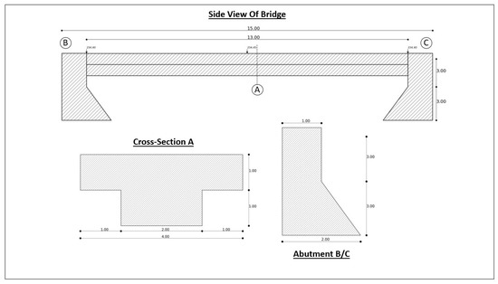
Figure 1. A sample of a side view of a bridge, showing the details of the cross-section of the upper structure and the abutment. The side view shows how the various parts come together to form the bridge.

For calculating the scale S a distance between two pixel locations within the ROI is measured. The recommended pixel locations for computing the pixel distance includes clearly defined markers and straight edges with corresponding metric dimension from the plan. The pixel-to-meter scale S is then computed using the pixel distance and the corresponding distance in meters from the plan.

Using Optical Character Recognition, texts and location of the text are detected within the ROI. The OCR algorithm used is based on [13]. The OCR algorithm identifies the characters of the text, the locations (bounding box) of the characters and an estimated accuracy of the predicted characters. The identified characters within the bounding boxes are removed.

2.1.2. Estimate Corners

This is a semi-automated process to estimate corners of the part to be reconstructed within the ROI as shown in Figure 2. First, we estimate the perimeter using topological structural analysis [14] of a binary image. The second step uses a line simplification algorithm, such as Visvalingam’s algorithm, [15] and Douglas–Peucker [16] is used to decimate smaller curve composition for the estimated corner points. The Douglas-Peucker algorithm implemented in OpenCV is used in this paper to remove falsely estimated corner points ${\mathbf{p}}_{\mathbf{i}}$.

$${\mathbf{p}}_{\mathbf{i}}=(x_i,y_i)$$

(1)

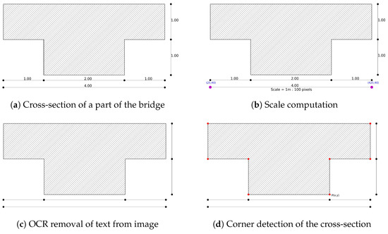
Figure 2. Describes the workflow of the feature extraction. (a) is the cropped-out image; (b) explains the scale computation from the pixel coordinate system and a metric coordinate system; (c) shows the result after removing the text from the image using OCR; the red dots in (d) indicate the corners $\mathbf{P}(\mathbf{x},\mathbf{y})$ of the cross-section.

The final step is to manually validate or confirm which corners belong to the part to be reconstructed within the ROI. This step is necessary to remove false corners, which are estimated due to shading or noise on the image. Alternatively, the undetected corners can be added during this process. The final output of the process is a list of n corner points $\mathbf{C}$ that define the part of the bridge to be reconstructed.

$$\mathbf{C}=\{{\mathbf{p}}_{\mathbf{1}},{\mathbf{p}}_{\mathbf{2}},{\mathbf{p}}_{\mathbf{3}}\cdots {\mathbf{p}}_{\mathbf{n}}\}$$

(2)

As mentioned above, the corner estimation is highly influenced by the quality of the input image (resolution, contrast, sharp edges, etc.). Especially for low-resolution images, i.e., below 100 dpi, false corners are detected. The false corners predictions can be removed. In our example, the number of estimated corners varies between 146 (for 20 dpi) and 8 (for 100 dpi); true value was 8—see Figure 3. Additionally, lines or handwritten text, created accidentally or intentionally, have no effect on the corner estimation process—see Figure 4.

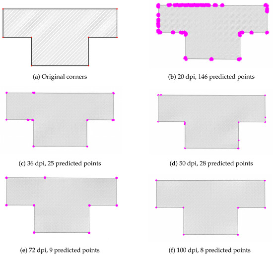
Figure 3. Detection of corners determined from the resolution of scanned cross-section; (a) shows the corners as designed by the CAD model; (b–f) show the corner estimation at various resolutions.

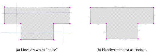
Figure 4. Influence of “noise” on the detection of the corner points; (a) shows lines drawn over the cross-section; (b) shows handwritten text on cross-section.

2.2. 3D Point Cloud Reconstruction

We derive 3D point cloud of the object as an intermediate step on the way to a 3D model. Our method is based on the work done by [9]. A 3D point cloud of the object will support the use of other geo-referenced measurements, e.g., multi-spectral camera streams, data from laser scanning, etc. [2,17].

A basic understanding of the bridge and building plan is required to extract additional measurements needed for deriving the 3D point cloud. The list of $\mathbf{n}$ corner points $\mathbb{c}$ of the part of the bridge to be reconstructed from the previous section is converted from the image coordinate (in pixels and 2D) to absolute coordinates (in meters and 3D). The first step involves scaling using the computed scale S to obtain the corner points C in meter. Additionally, an initial value z is added to the third dimension to create 3D points for all corners.

$$\begin{array}{cc}\hfill {\mathbf{p}}_{\mathbf{i}}& =(x_i*S,y_i*S,z)\hfill \\ \hfill {\mathbf{p}}_{\mathbf{i}}& =(\widehat{x_i},\widehat{y_i},z)\hfill \\ \hfill \mathit{C}& =\{{\mathbf{p}}_{\mathbf{1}},{\mathbf{p}}_{\mathbf{2}},{\mathbf{p}}_{\mathbf{3}},\cdots ,{\mathbf{p}}_{\mathbf{n}}\}\hfill \end{array}$$

(3)

The second step involves defining the length L and the curvature of the selected part of the bridge. The length L of the selected part is defined based on the plans. Some parts of the bridge, such as the superstructure, are designed with different elevations ${\mathbf{h}}_{\mathbf{i}}$. The change in elevation is responsible for the curvature. The list of elevations $\mathbf{H}$ along the specific point on the selected part ${\mathbf{h}}_{\mathbf{i}}$ is defined with respect to the plans. In this step, the desired resolution $res$, which is a variable parameter, is required as an input to compute the curvature. The curvature between the list of elevations $\mathbf{Elev}$ is computed using a Cubic Spline interpolation [18]. This method uses cubic functions to interpolate the elevations.

$$\begin{array}{cc}\hfill H& =(h_0,h_1,h_2,\cdots ,h_n)\hfill \\ \hfill L_{interval}& =\{l_o,l_o+res,l_{i-1}+res,\cdots ,L\}{l}_o=0\hfill \\ \hfill \mathbf{Elev}& =\mathbf{CubicSpline}(L_{interval},H)\hfill \end{array}$$

(4)

In the next step, we reconstructed the point cloud using the defined length L, the estimated elevation $\mathbf{Elev}$ and the corner points $\mathbf{C}$. This is an iterative process with an increment interval of the defined resolution $res$ to create layers of point clouds from 0 until the length L. A layer of the point cloud is generated by discretizing three-dimensional points between two corner points at an interval of the resolution $res$ defined. The discretized points form a point cloud, which defines the periphery of the polygon of the selected part at the length interval ${\mathbf{l}}_{\mathbf{i}}$. The layers from each length interval ${\mathbf{l}}_{\mathbf{i}}$ are stacked together to create an enclosed 3D point cloud object, as shown in Figure 5d. Points are generated between the corner points $\mathbf{C}$ at a resolution $res$ defined to create the periphery of the polygon of the selected part.

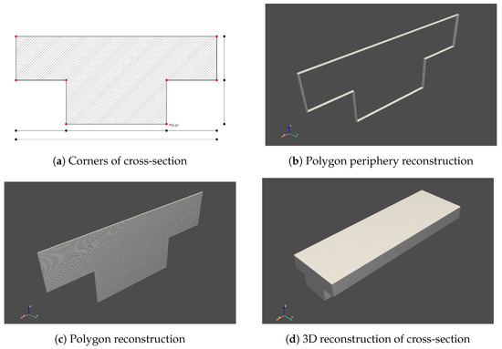
Figure 5. point cloud reconstruction of the (a) ROI selected; (b) shows the periphery point cloud of the polygon and (c) shows a fully filled point cloud of the polygon; (d) is a stack of layers of point cloud.

At the beginning and end of the part of the bridge to be reconstructed, a fully filled polygon layer of point cloud, as shown in Figure 5c, is generated. This layer is generated by further generating points within the peripheral polygon initially generated. This is also achieved at the same interval of the resolution $res$ defined to create the point cloud. In between the two layers at the ends, a point cloud of the periphery of the polygon reconstructed, as shown in Figure 5b, at the same resolution. This process creates a hollow reconstruction of the part that replicates the surface of the object, as shown in Figure 5d.

After each point cloud layer reconstruction, the elevation is updated with the estimated elevation $\mathbf{Elev}$ at the particular length.

This update creates the curvature when all the layers are stacked together to form the complete 3D point cloud.

One of the main parameters needed for the 3D reconstruction is the choice of resolution. The resolution influences the number of points generated during the reconstruction process. This affects the runtime of the process and the memory size of the generated file. The selection of the resolution is dependent on the application of the reconstructed model. For example, if the reconstructed point cloud is to be fused with a laser scanner’s point cloud, a high resolution is recommended. Resolutions varying from 2 mm to 20 cm were selected for the reconstructed part of the bridge (2 m × 4 m × 13 m). The number of points and the corresponding runtime at each resolution are shown in Figure 6.

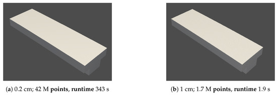
Figure 6. Various resolutions of the 3D reconstruction. The high resolutions shown in (a,b) show more points to clearly defined surfaces and edges. The medium resolutions shown in (c) show enough points to define the structure of the object. The low resolutions shown in (d) show less points describing the object. Resolution of 3D reconstruction.

Evaluation of 3D Model

We compared the reconstructed point cloud dimensions with the dimensions from the plans to evaluate the evaluation process. The dimension of the 3D point cloud reconstructed at a resolution of 2 cm was calculated using the CloudCompare distance computation tool. The distances between the points located at the corners of the point cloud were measured and compared to the designed dimensions from the plans. The measured distances from the point cloud matched the designed dimension from the plan, as shown in Figure 7b.

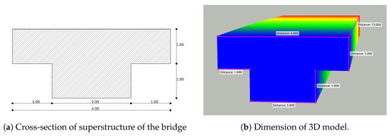
Figure 7. Comparison of the dimension of the 3D reconstructed point cloud (b) and the designed dimension from the plan (a); the depth of the point cloud is described with blue-red color-scale from 0 to 13 m.

2.3. Fusion of Reconstructed Bridge Parts

In this step, the various selected reconstructed parts are registered into one coordinate system based on the plans. This process also requires some knowledge and understanding in the interpretation of the 2D plans. A view from the plan with all the reconstructed parts is recommended to be used to fuse them. To begin, a local coordinate system is defined based on the main components of the bridge; for example, the superstructure can be used as the reference. The fusion process involves using a third-party software, i.e., CloudCompare, to register the various parts together.

Alternatively, transformation parameters can be estimated to register the parts reconstructed using keypoints. This process is recommended in the case where a reference image cannot be directly derived from the 2D plans. The keypoints may include corners and planes that can be used to register parts to fuse the reconstructed parts together.

The fusion process of the various individual parts to create a complete reconstruction as shown in Figure 8 could be computationally expensive and require more time. For this reason, it is recommended to register the individual parts with respect to the reference one reconstructed part at a time. In addition, depending on the resolution of the reconstructed model, to fuse the individual parts into one 3D object, it is recommended to downsample the point cloud and crop out duplicate points on the intersecting planes.

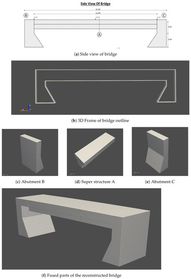
Figure 8. 3D point cloud fused from the various parts. (a) is used as the reference to generate (b) a 3D frame of the bridge for the fusion of (c–e) to create (d) a fully reconstructed bridge.

3. Results

The 3D reconstruction process was tested with three bridges: Gaskugel bicycle bridge, Max-Müller-Steg and Ottiliensteg over the Dreisam river in Freiburg, Germany. All the 2D bridge plans were provided by the state authority in charge of the bridges in Freiburg: Stadt Freiburg im Breisgau, Garten- und Tiefbauamt, Verkehrswegebau/Ingenieurbauwerke. The three bridges provided different scenarios to test the 3D reconstruction process. The bridges were reconstructed to scale with the same dimensions on the plans with a standard deviation of the defined resolution. In the following subsections, the outputs for each of the bridges are described.

3.1. Gaskugel Bicycle Bridge

The Gaskugel bicycle bridge in the west of Freiburg crosses the Dreisam river. It comprises four main parts: the north and south abutments, the concrete superstructure and the steel metallic reinforcement substructure. The dimension of the bridge is 7.5 m, 39.7 m and 5.6 m in width, length and height, respectively. The state office in charge of the bridges provided eight 2D plans of various parts of the bridge that were used to reconstruct the 3D models as shown in Figure 9.

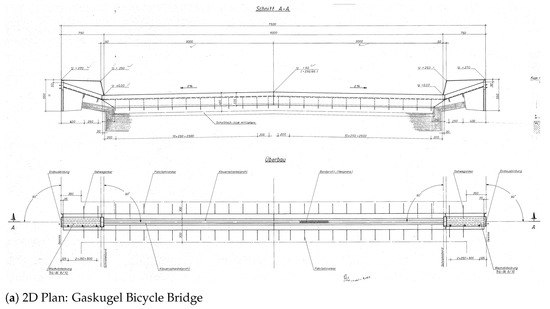
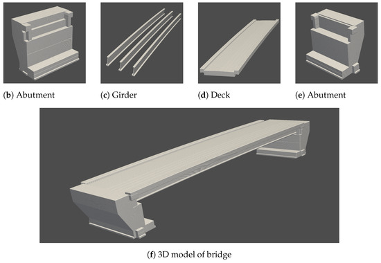
Figure 9. 3D reconstruction of Gaskugel bicycle bridge over the Dreisam river in Freiburg. (a) is one of the eight 2D plans used to reconstruct some parts of the 3D model of the bridge. (d) is a 3D reconstruction of the concrete superstructure of the bridge. (c) is a 3D reconstruction of the metallic reinforcement of the bridge. (b,e) are 3D reconstructions of the abutments of the bridge. (f) depicts the fused parts of the reconstructed 3D model of the Gaskugel bicycle bridge.

The Gaskugel bicycle bridge 3D reconstructed model comprises about 80% of the entire bridge. This 3D reconstructed model excludes the sidewalk rails and some additional metal work parts of the re-enforcement steel base. These parts were not available in the provided plans of the bridge.

3.2. Max-Müller-Steg

The Max-Müller-Steg is located in the eastern part of Freiburg and crosses the Dreisam river. It comprises three main parts: the north and the south abutment and the superstructure. The dimensions of the bridge are 2.8 m, 29.8 m and 2.95 m in width, length and height, respectively. The state office in charge of the bridges provided five 2D plans of various parts of the bridge that were used to reconstruct the 3D models, as shown in Figure 10. The bridge rails on each side of the bridge were also reconstructed as part of the superstructure of the bridge.

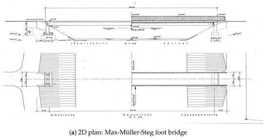
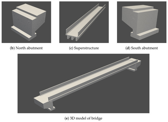
Figure 10. 3D reconstruction of Max-Müller-Steg foot bridge over the Dreisam river in Freiburg. (a) is one of the five 2D plans used to reconstruct the parts of the 3D model. (c) is a 3D reconstruction of the concrete superstructure of the bridge. (b,d) are 3D reconstructions of the north and south abutments of the bridge. (e) shows the fused parts of the reconstructed 3D model of the Max-Müller-Steg foot bridge.

The Max-Müller-Steg reconstructed point cloud comprises approximately 90% of the bridge with the exception of the approach embankment. The superstructure consists of three longitudinal girders, kerb, deck slab and handrails. The handrails were reconstructed as a solid surface without the gaps between the rails.

3.3. Ottiliensteg

The Ottiliensteg is located in the eastern part of Freiburg and crosses the Dreisam river. It comprises three main parts: the north and south abutments and the concrete superstructure. The dimensions of the bridge are 2.28 m, 34.80 m and 3.5 m in width, length and height, respectively. The state office in charge of the bridges provided a single sheet 2D plan of various parts of the bridge that was used to reconstruct the 3D models, as shown in Figure 11. The bridge rails on each side of the bridge were also reconstructed as part of the superstructure of the bridge.

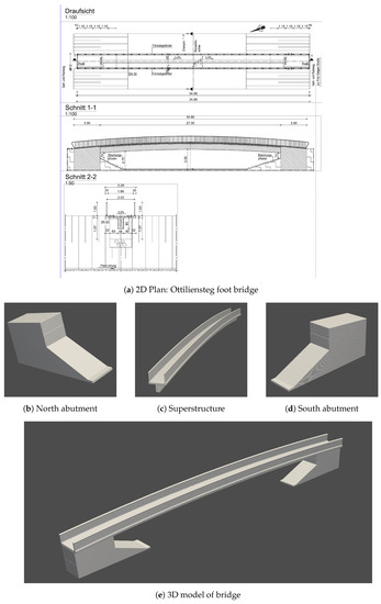
Figure 11. 3D reconstruction of Ottiliensteg foot bridge over the Dreisam river in Freiburg. (a) is the 2D plan used to reconstruct the parts of the 3D model. (c) is a 3D reconstruction of the concrete superstructure of the bridge. (b,d) is a 3D reconstruction of north and south abutments of the bridge. (e) shows the fused parts of the reconstructed 3D model of the Ottiliensteg foot bridge.

The Ottiliensteg reconstructed point cloud comprises almost the entire bridge as designed in the plan. The superstructure includes a single longitudinal girder, kerb, handrails and a deck slab. The handrails were reconstructed as a solid surface without the gaps between the rails. The substructure also includes the approach embankment and the abutments.

4. Conclusions

This study presents a semi-automated method for reconstructing bridges in 3D from hand-drawn and computer-drawn plans. The process provides a completely fused point cloud of a bridge, including parts that are not visible in the as-built measured point cloud of the bridge. This provides an intermediary object of a 3D model for various BIM applications, such as monitoring and evaluation of bridges. Point clouds from laser scanners and photogrammetry techniques are limited in terms of reconstructing structures below the deck and the substructure of a bridge due to occlusions. The point clouds of a bridge reconstruction in this study, therefore, represent a useful complement to circumvent these limitations.

In the future, we will research the fusion of the 3D reconstructed point cloud and the as-built photogrammetry and laser scan point cloud. The objective is to extend the research to other architectural structures, such as buildings.

References

- Li, J.; Huang, W.; Shao, L.; Allinson, N. Building recognition in urban environments: A survey of state-of-the-art and future challenges. Inf. Sci. 2014, 277, 406–420. [Google Scholar] [CrossRef]
- Goebbels, S. 3D Reconstruction of Bridges from Airborne Laser Scanning Data and Cadastral Footprints. J. Geovisualization Spat. Anal. 2021, 5, 1–15. [Google Scholar] [CrossRef]
- Koutamanis, A.; Mitossi, V. Automated recognition of architectural drawings. In Proceedings of the 1992 11th IAPR International Conference on Pattern Recognition, IEEE Computer Society, Hague, The Netherlands, 30 August–3 September 1992; Volume 1, pp. 660–663. [Google Scholar]
- So, C.; Baciu, G.; Sun, H. Reconstruction of 3D virtual buildings from 2D architectural floor plans. In Proceedings of the ACM Symposium on Virtual Reality Software and Technology, Taipei, Taiwan, 2–5 November 1998; pp. 17–23. [Google Scholar]
- Yin, X.; Wonka, P.; Razdan, A. Generating 3d building models from architectural drawings: A survey. IEEE Comput. Graph. Appl. 2008, 29, 20–30. [Google Scholar] [CrossRef] [PubMed]
- Gimenez, L.; Robert, S.; Suard, F.; Zreik, K. Automatic reconstruction of 3D building models from scanned 2D floor plans. Autom. Constr. 2016, 63, 48–56. [Google Scholar] [CrossRef]
- Zhu, J.; Zhang, H.; Wen, Y. A new reconstruction method for 3D buildings from 2D vector floor plan. Comput.-Aided Des. Appl. 2014, 11, 704–714. [Google Scholar] [CrossRef]
- Lipson, H.; Shpitalni, M. Optimization-based reconstruction of a 3D object from a single freehand line drawing. In Proceedings of the ACM SIGGRAPH 2007 Courses, San Diego, CA, USA, 2–4 August 2007; p. 45. [Google Scholar]
- Xue, T.; Liu, J.; Tang, X. Example-based 3D object reconstruction from line drawings. In Proceedings of the 2012 IEEE Conference on Computer Vision and Pattern Recognition, Providence, RI, USA, 16–21 June 2012; pp. 302–309. [Google Scholar]
- Yang, L.; Liu, J.; Tang, X. Complex 3d general object reconstruction from line drawings. In Proceedings of the IEEE International Conference on Computer Vision, Sydney, Australia, 1–8 December 2013; pp. 1433–1440. [Google Scholar]
- Wang, F.; Yang, Y.; Zhao, B.; Jiang, D.; Chen, S.; Sheng, J. Reconstructing 3D model from single-view sketch with deep neural network. Wirel. Commun. Mob. Comput. 2021, 2021. [Google Scholar] [CrossRef]
- Wang, L.; Qian, C.; Wang, J.; Fang, Y. Unsupervised learning of 3D model reconstruction from hand-drawn sketches. In Proceedings of the 26th ACM International Conference on Multimedia, Seoul, Republic of Korea, 22–26 October 2018; pp. 1820–1828. [Google Scholar]
- Jaided. GitHub-EasyOCR. 2021. Available online: https://github.com/JaidedAI/EasyOCR (accessed on 3 August 2022).
- Suzuki, S. Topological structural analysis of digitized binary images by border following. Comput. Vision Graph. Image Process. 1985, 30, 32–46. [Google Scholar] [CrossRef]
- Visvalingam, M.; Whyatt, J.D. Line generalization by repeated elimination of points. In Landmarks in Mapping; Routledge: London, UK, 2017; pp. 144–155. [Google Scholar]
- Ramer, U. An iterative procedure for the polygonal approximation of plane curves. Comput. Graph. Image Process. 1972, 1, 244–256. [Google Scholar] [CrossRef]
- Pepe, M.; Costantino, D. UAV photogrammetry and 3D modelling of complex architecture for maintenance purposes: The case study of the masonry bridge on the Sele river, Italy. Period. Polytech. Civ. Eng. 2021, 65, 191–203. [Google Scholar] [CrossRef]
- De Boor, C.; De Boor, C. A Practical Guide to Splines; Springer: New York, NY, USA, 1978; Volume 27. [Google Scholar]
Disclaimer/Publisher’s Note: The statements, opinions and data contained in all publications are solely those of the individual author(s) and contributor(s) and not of MDPI and/or the editor(s). MDPI and/or the editor(s) disclaim responsibility for any injury to people or property resulting from any ideas, methods, instructions or products referred to in the content. |
© 2023 by the authors. Licensee MDPI, Basel, Switzerland. This article is an open access article distributed under the terms and conditions of the Creative Commons Attribution (CC BY) license (https://creativecommons.org/licenses/by/4.0/).