Abstract
Mangrove wetlands are rapidly being lost due to anthropogenic disturbances and natural processes, such as sea-level rise (SLR), but are also recovering as a result of conservation efforts. Accurate and contemporary mangrove maps to detect their distribution and changes are urgently needed to understand how mangroves respond to global change and develop effective conservation projects. Here, we developed a new change detection algorithm called temporal consistency checking combining annual classification and spectral time series (TCC-CS) for tracking mangrove losses and gains. Specifically, mangrove change events were determined by measuring the deviation of greenness and wetness of candidate change segments from automatically collected mangrove reference samples. By applying to the world’s largest mangrove patches, we monitored the 35-year mangrove trajectory in the Sundarbans from 1988 to 2022 using all available Landsat images on the Google Earth Engine platform. In the Sundarbans, 18,501.89 ha of mangroves have been gained, but these have been offset by losses of 27,009.79 ha, leading to a net mangrove loss of 1.42% (8507.9 ha) in the past 35 years. We further mapped the pixel-level change agents and found that SLR-induced erosion and degradation, instead of human activities, were the major drivers of losses in the Sundarbans. Trend analysis on loss agents indicates that mangrove losses caused by human activities, such as the expansion of croplands and aquaculture ponds, have declined, but SLR is still a persistent threat to mangrove wetlands in this iconic mangrove area. Our study provides a computationally efficient methodology for examining large-scale mangrove changes, and the resultant annual mangrove maps provide strong support for mangrove conservation in the Sundarbans.
1. Introduction
Mangrove forests play a critical role in the global carbon cycle through their high productivity and substantial blue carbon pools [1,2] and a functional link between terrestrial and marine realms by receiving land-source carbon inputs and exporting carbon towards the open ocean [3]. However, their spatial extent is highly dynamic, with unprecedented losses from deforestation and sea-level rise (SLR) [4]. Indeed, increases in aquaculture, urban areas, and agricultural activities have transferred a lot of mangrove forests to anthropogenic landscapes [5,6], accounting for 62% of global mangrove losses [4], with annual deforestation rates between 0.16% and 0.39% since 2000 [7]. Recent actions have called for ambitious mangrove conservation and restoration targets at regional, national, and global scales to counteract the rapid mangrove loss [8], which have paid off with substantial mangrove gains in some countries such as China [9]. Hence, understanding the annual dynamics in mangrove cover is pivotal to identifying priorities for future mangrove restoration and assessing the effectiveness of the current conservation efforts.
Satellite-based remote sensing observation provides an effective and viable way to monitor mangrove changes at the regional or larger spatial extents over a long period, which is challenging if using ground-based investigations and field surveys due to the high cost of comprehensive mapping and inaccessibility of intertidal environments [10]. Methodologies in detecting mangrove changes by satellite remote sensing can generally be grouped into two types: post-classification comparison and spectral time-series anomalies.
Post-classification comparison detects change areas by contrasting mangrove extents at different time points (i.e., classification before change detection). Often, this approach involves mangrove classification at different years using medium-resolution satellite data, such as Landsat [11] and Sentinel-2 [12]. It performs well when the mangrove extent maps are accurate but is particularly sensitive to errors embedded in each mangrove map and therefore suffers from error propagation [13,14]. Its temporal frequency is commonly low, such as once classification per 5 or 10 years [12,13], to mitigate total errors in mangrove maps. Instead, detecting changes through spectral time-series anomalies usually tracks where and when changes happened first and classifies each temporal segment to a specific land-cover type as a later step (i.e., detecting changes and then classification) [13,14,15]. This kind of approach can detect complete changes but requires high-quality time-series observations at a high temporal frequency. However, since mangroves are located in low-latitudinal tidal areas with frequent cloud cover and inundation [16], their time-series spectral observations are usually noisy, with many false changes. Detecting changes from time-series mangrove observations thus may suffer from the inherently dynamic nature of mangrove wetlands and have large commission errors [17].
As the world’s largest single tract of continuous mangrove forests, the Sundarbans presents an excellent example of ongoing mangrove dynamics. Several studies [18,19,20] have observed the overall stable areal extent of mangrove forests in the Sundarbans, and the net loss area accounted for only approximately 1.2% of the total mangrove area during the recent decades, but the turnover between mangrove losses and gains is much greater, mainly due to erosion and accretion. Although changes in the Sundarbans mangroves have been successfully observed, previous studies have mainly relied on differencing multi-date mangrove classification at a 5 or 10 year frequency, failing to detect mangrove changes at an annual scale and thus are incapable of tracking the long-term trend of changes and causes.
Here, our goal is to map and characterize changes in the Sundarbans mangrove forests from 1988 to 2022 at an annual scale. Specifically, we aimed: (1) to develop a new algorithm for tracking mangrove changes at an annual frequency by integrating classification differencing and spectral time-series anomaly detection, (2) to describe the spatio-temporal pattern of mangrove changes in the Sundarbans, and (3) to map the mangrove change agents and quantify their long-term trends.
2. Materials and Methods
2.1. Study Area
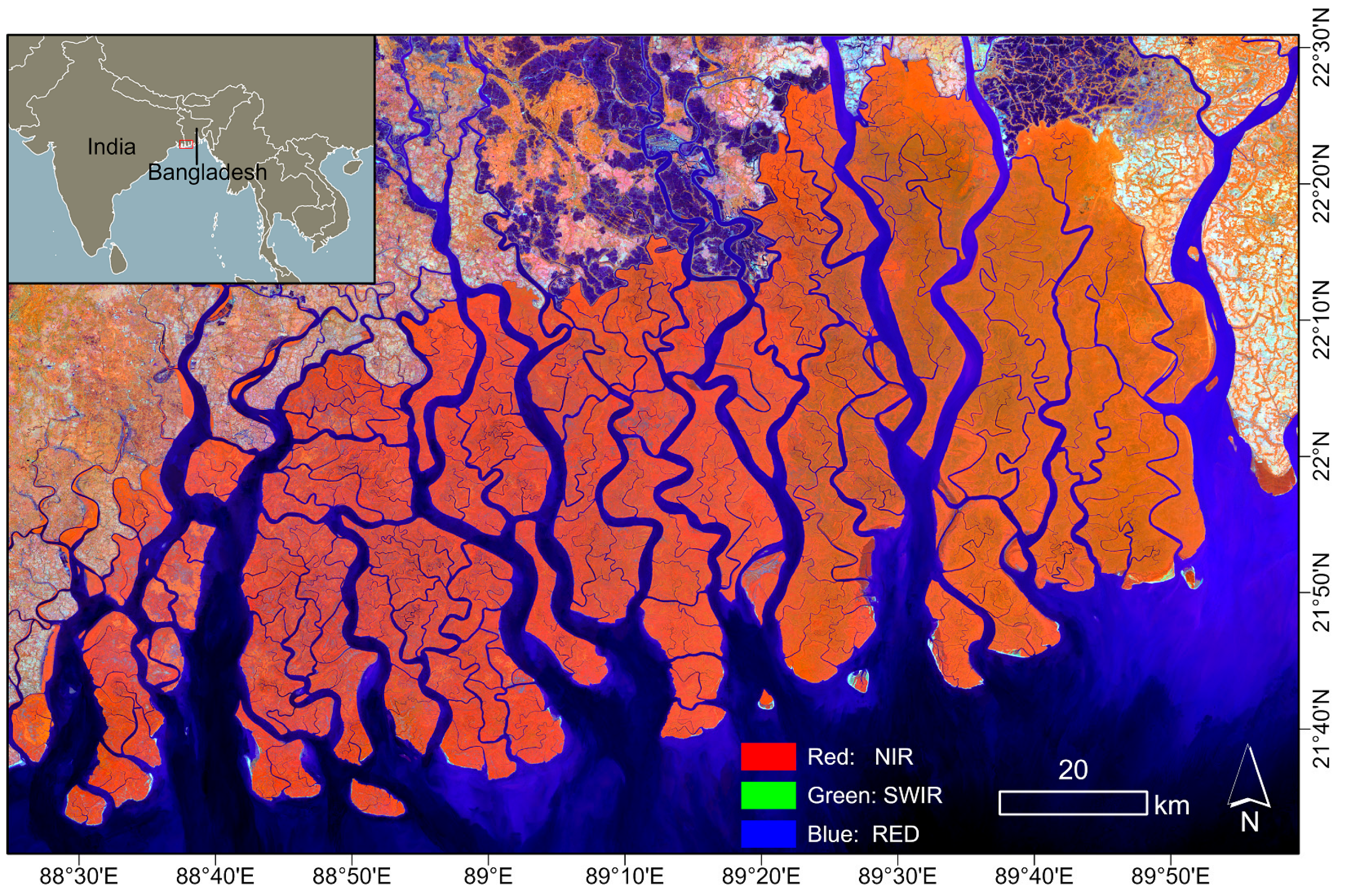
We focused our research on the Sundarbans mangrove forests (Figure 1), which are distributed from the Hooghly river in the west to the Baleswar river in the east, encompassing the India–Bangladesh border with 62% in Bangladesh and 38% in India [21], split by numerous tidal channels and creeks. The area experiences a tropical monsoon climate, characterized by a mean minimum and maximum temperature between 21 °C and 35 °C and an average annual rainfall between 1500 mm and 1800 mm [22], with a wet season between March to November. The Sundarbans mangroves hold a wide range of flora and fauna, including 27 true mangrove taxa and 40 species of mammals, such as the Bengal tiger [18,23]. Given its high ecological importance, the Sundarbans mangrove forests have been the focus of increased conservation attention since the establishment of the Sundarbans Biosphere Reserve in 1997.
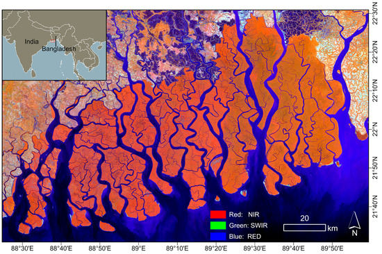
Figure 1.
Map of the study area and its location encompassing the India–Bangladesh border. The false-color (near-infrared (NIR), shortwave infrared band 1 (SWIR), and red bands as RGB) image was obtained from Landsat-8 median composite in 2022.
2.2. Landsat Imagery and Pre-Processing
The Sundarbans mangrove forests are intersected within the Landsat scenes 137–138/44–45 (paths/rows). The complete Landsat archive of Thematic Mapper (TM), Enhanced Thematic Mapper Plus (ETM+), and Operational Land Imager (OLI) images from January 1988 to December 2022 over the study region was acquired and processed on the Google Earth Engine (GEE) platform [24], yielding 2624 multi-band surface reflectance (SR) Landsat measurements, of which 1555 (59%) were considered to be useable (cloud cover < 30%) based on the quality assurance band provided by the CFmask algorithm [25]. Median composites were generated for each year to obtain cloud-free Landsat images and to fix our analysis on the relatively stable water level. Due to the sensor differences between ETM+ and OLI and sufficient observations of Landsat-8, only the Landsat-8 OLI images were used since 2013. The average cloud-free observations per year were 427, with a standard deviation of 155 (Figure 2a). Figure 2b shows the number of used Landsat observations for each year.

Figure 2.
The number of good Landsat observations used to map mangrove change. (a) The spatial distribution of total cloud-free Landsat observations from 1988–2022, which provides pixel-level details of how many Landsat observations were available for classification. (b) Numbers of clear images (cloud coverage < 30%) by Landsat sensors for each year.
2.3. Mapping Mangrove Extent for Each Year
2.3.1. Collecting Unchanged Training Samples
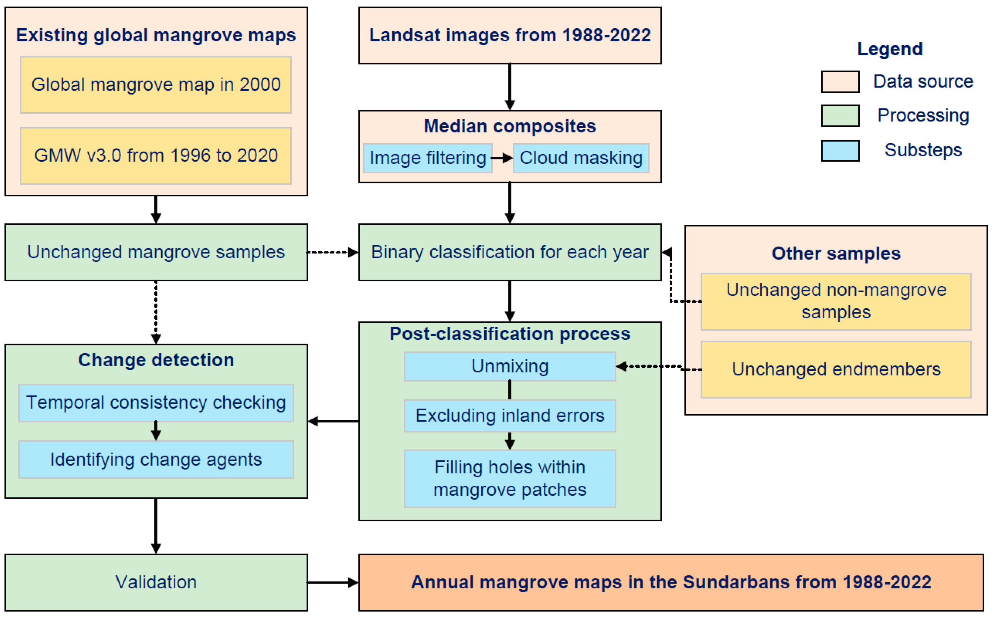
For detecting the mangrove change area, the first step in this study was to map the mangrove distribution for each year (Figure 3). The supervised strategy was chosen for classification due to its reliable performance. However, supervised classification requires abundant training samples, which are labor-intensive to collect, especially for an annual classification task [26]. Thus, we collected unchanged training samples for the classification each year, comprising two types: mangroves and non-mangroves.
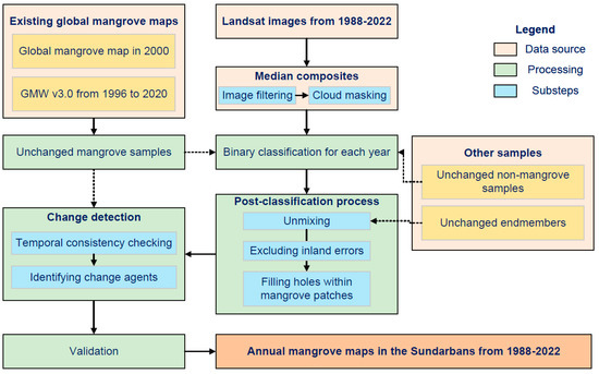
Figure 3.
Methodological workflow for the detection of mangrove changes.
The unchanged mangrove samples were collected from existing global mangrove products, including Giri’s global mangrove map in 2000 [27] and Global Mangrove Watch version 3.0 [28] from 1996 to 2020. Specifically, we randomly selected 100 points within the intersection parts of these mangrove maps and then generated a buffer around these points with a radius of 300 meters (i.e., the length of 10 Landsat pixels) to increase the total number of training samples [4]. The intersections between the buffers and the mangrove intersection map (i.e., the mangrove part within these buffers) were considered the initial unchanged mangrove samples. Since the mangrove intersection map has different periods with this study (1996–2020 vs. 1988–2022) and may have misclassification errors, we updated the initial unchanged mangrove samples to each year by eliminating pixels having abnormally low greenness, considering that mangroves are evergreen broadleaf woody plants and usually have high greenness. In detail, we calculated the NDVI z-score for each Landsat pixel from the initial unchanged mangrove samples and eliminated pixels with NDVI z-scores below −2 [29]. The NDVI z-score measures the degree to which the pixel deviates from the mangrove samples. Only 2.28% of the data-point’s z-scores lie below −2 if the data follow a Gaussian distribution, so −2 is often selected as the threshold to detect statistical outliers. The pixels within the intersection area of these annual mangrove samples were finally determined as the unchanged mangrove samples.
The unchanged non-mangrove samples consist of five sub-classes, including inland forests, croplands, water, tidal flats, and impervious surfaces. We manually collected 50 unchanged polygons for each subclass by referring to the median Landsat composites in the first year (1988), the median year (2005), and the last year (2022). Together with the unchanged mangrove samples, these unchanged non-mangrove samples were applied as training samples for subsequent annual supervised classifications.
2.3.2. Binary Supervised Classification
An annual supervised classification was conducted on GEE by classifying every Landsat pixel to either mangroves or non-mangroves. This binary strategy, compared to multi-class classification (i.e., mangroves and multiple non-mangroves subclasses), could improve classification accuracy even with fewer training samples [30]. The commonly used random forest (RF) was used as the classifier due to its high accuracy and robustness [31]. The parameter NTrees (the number of trees) in RF was set as 200 according to our previous experiment on mapping tidal wetlands [16]. To help distinguish mangroves and other land-cover types, several quantile composites of Landsat images were concatenated as the final image for classification, including 10%, 25%, median, 75%, and 90%. These quantile composite images represented different phenological stages and water levels, providing extra information for the classification compared to using only a median image [32,33]. Specifically, all spectral bands at a 30 m resolution and several spectral indices of these quantile composite images (listed in Table 1) were used in the classification.

Table 1.
Spectral indices used in the classification.
2.3.3. Post-Processing
After running the binary supervised classification, three procedures were performed to improve the annual classification results:
- Reserving vegetation-dominated pixels: The vegetation–water mixture is the main commission error source in mapping mangroves [33,44]. As a hard-classification study, the resulting mangrove pixels are expected to be dominated by vegetation. As such, we manually selected 60 unchanged endmembers during 1988–2022 and performed the linear unmixing technique for each year, estimating the percentage of sub-pixel vegetation, water, and bare soil coverages. Only pixels classified as mangroves with the largest vegetation proportion were retained. This step could eliminate commission errors distributed along the edges between mangroves and water bodies;
- Eliminating inland errors: Dense inland forest is another main commission error source [44]. Inland commission errors were filtered out by intersecting the classification results with those existing mangrove products (i.e., Giri’s mangrove map and GMW v3.0). Specifically, we used the union of existing mangrove products as the initial maximum mangrove extent (MME), which was intersected with our mangrove classification results in 1988, 2005, and 2022 (i.e., the first, median, and last years) to identify the true mangrove areas in these three years. Considering this MME layer may omit some mangrove areas due to the period mismatch (1988–2022 vs. 1996–2020 of GMW), we manually retained those mangrove patches that were not intersected by the MME layer in the three years. The union of the filtered mangrove areas in the three years was used as the final MME during 1988–2022, which was intersected with our mangrove results in other years to exclude inland errors;
- Filling holes within mangrove patches: Lastly, the holes within the mangrove patches were filled to mitigate omission errors. Our assumption is that the holes surrounded by mangroves are either omission errors or low-vegetation-cover forest gaps. Thus, we checked the NDVI values of each hole pixel and filled areas with high-enough NDVI (i.e., NDVI z-score > −2) and the highest vegetation proportion (to ensure they are vegetation-dominated areas). Through these three steps, high-quality annual mangrove maps could be generated with minimized commission and omission errors.
2.4. Mangrove Change Detection
2.4.1. Temporal Consistency Checking
Considering changes by contrasting between classifications at two points in time may be false-positive due to the error propagation, we checked the temporal contexts of every potential change pixel (i.e., pixels with classification differences). Most existing temporal consistency checking (TCC) approaches are solely based on temporal classification results [45,46], ignoring the consistency of time-series spectral signals. Here, we developed a new strategy (Figure 4) based on time-series of both classification results and spectral signals (mainly NDVI and wetness in this study) to detect the true change, called the TCC-CS algorithm:
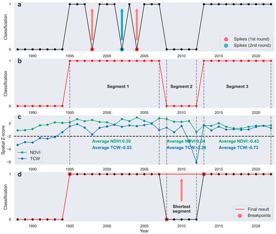
Figure 4.
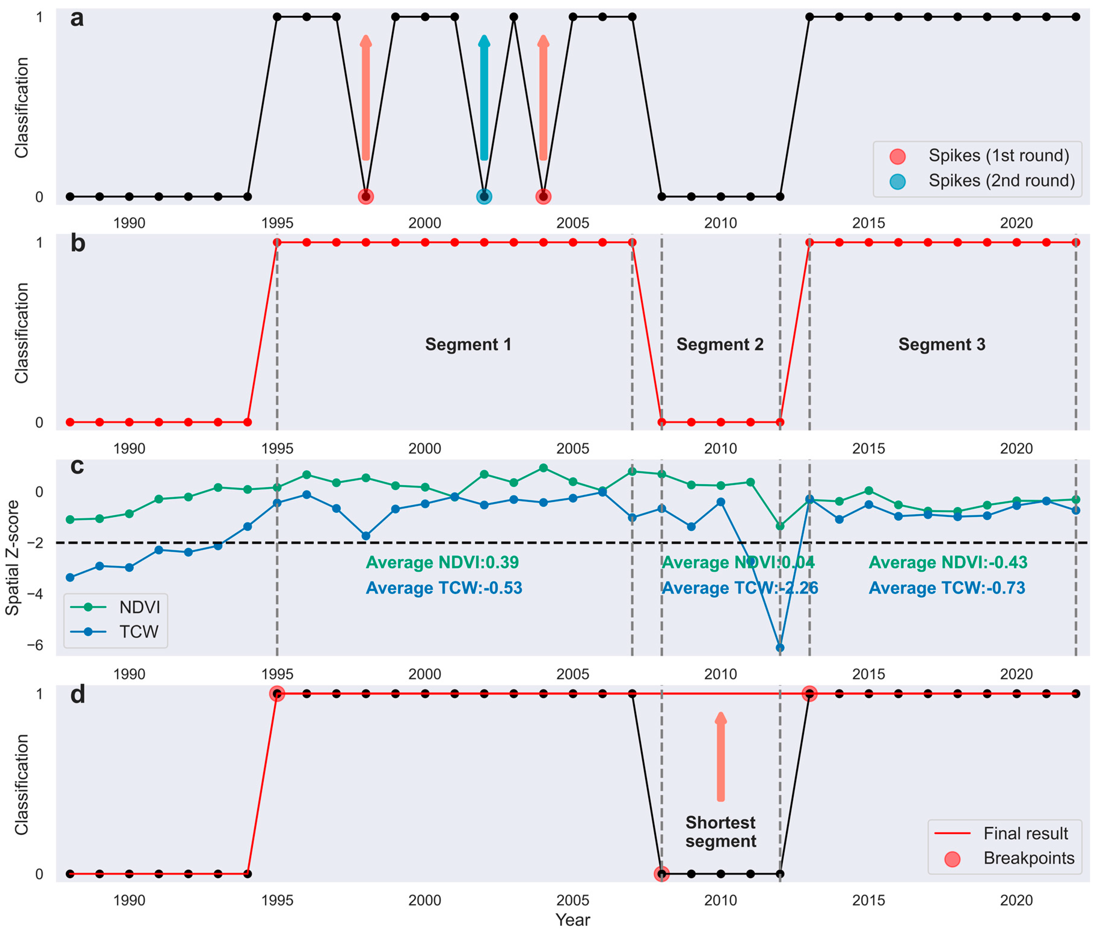
Annual classification results corrected by TCC-CS over a selected site (latitude: 22.385418°N, longitude: 89.646424°E). Spikes in the (a) raw classification results were iteratively corrected first. (b) Temporal segments were then corrected by their (c) average z-score of NDVI and TCW, generating the black line in (d). Since the breakpoints were more than 2, the shortest segment was corrected to its opposite state. Eventually, a mangrove gain event was detected in 1995.
- Correcting ephemeral spikes: Real mangrove gains/losses are persistent, with different land-cover types before and after the change times. Therefore, spikes in the time-series classification trajectory are assumed to be classification errors induced by noise such as residual clouds, cloud shadows, or high tides. A three-year temporal window was used to determine the spikes, including the prior year and the following two years of the target year, and the spike length was set up to two, considering that two consecutive isolated classification results were also highly likely to be misclassified. The classification state of the detected spikes was corrected between mangrove (1) and non-mangrove (0) in chronological order (Figure 4a). This correcting process was iterated until no spikes occurred.
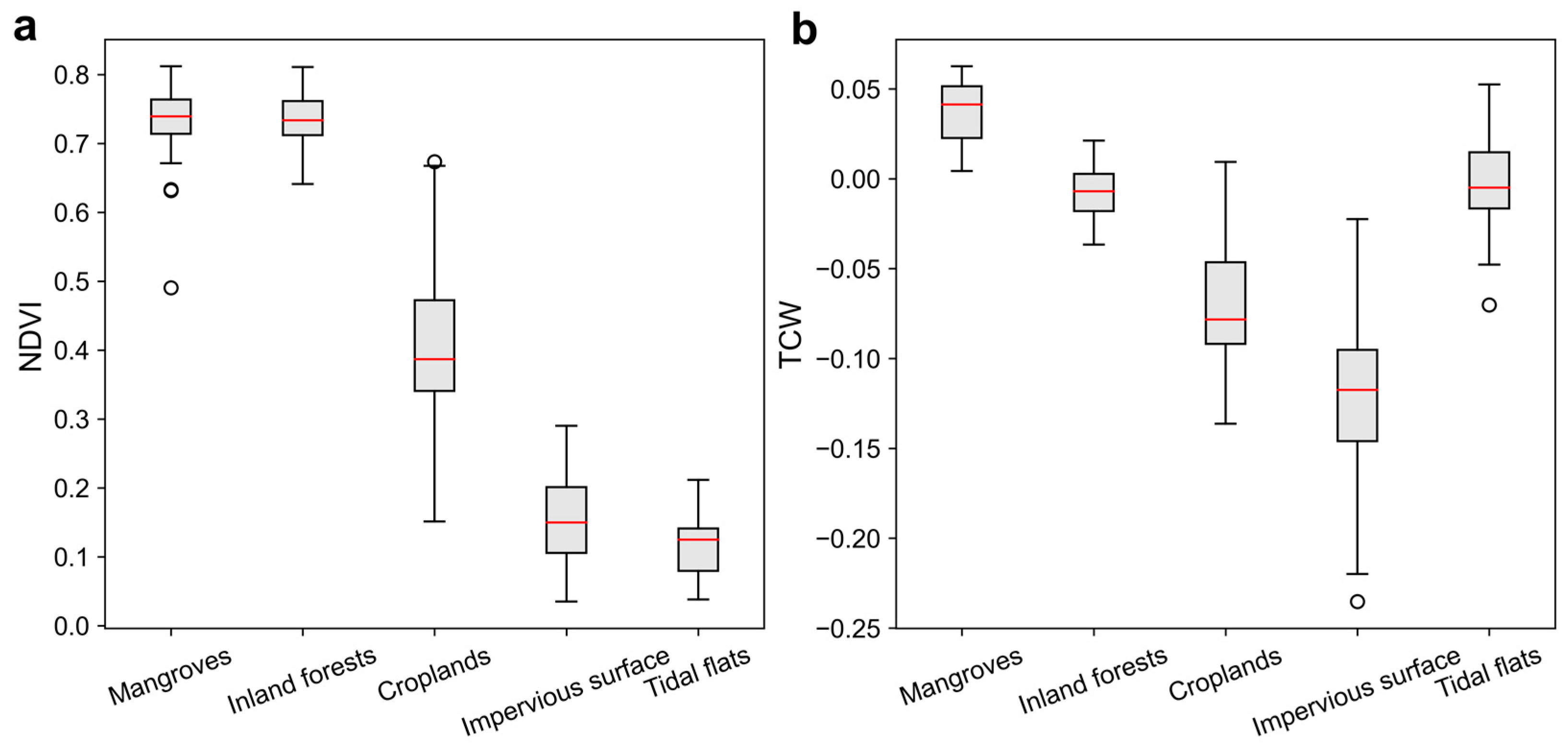
- Capturing spectral deviations relative to samples: Once the spikes within the classification time series were corrected, the trajectories of the classification results and spectral indices were divided into several segments according to the breakpoints (Figure 4b). Comparison analysis indicates that mangroves are the only land-cover type with high greenness and wetness in the study area (Figure 5). Therefore, mangrove segments should have both high greenness and wetness, and non-mangrove segments could have high greenness (inland forests) or high wetness (tidal flats), or neither (impervious surfaces). We compared the segments’ average NDVI and TCW spatial z-scores against a predefined threshold −2 to capture the spectral deviation (Figure 4c). In contrast to the commonly used temporal z-score, spatial z-score normalized the spectral signals to make the spectral trajectory more consistent across the sensors. Notice that if the breakpoint occurred in the first three years (i.e., 1989 and 1990), the detected change event might be false because the classification results before the breakpoint may contain errors (i.e., classification errors occurred in the first three years). For this situation, we additionally tested the segment before the breakpoint and corrected this to mangroves/non-mangroves if its average NDVI and TCW spatial z-scores were above/below −2.
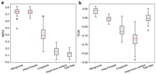 Figure 5. (a) NDVI and (b) TCW of five land-cover types. Boxes represent data within the 25th and 75th percentile, red lines show medians, and whiskers show 1.5× the interquartile range. Data points beyond that range (outliers) are shown as dots. Indices were collected from the Landsat-8 median composite in 2022.
 - Culling redundant breakpoints: In this case, 0.52% of the change pixels were detected to change more than twice after running the above correcting procedures. Since the transitions between mangrove and non-mangrove are unlikely to occur more than twice in a relatively short period, these breakpoints usually include false change events. For these trajectories with three breakpoints, the shortest temporal segment was corrected to the opposite state so that only one change was retained (Figure 4d). We observed that the pixels detected with more than three changes were almost all located at the edge of the mangroves (i.e., mixed pixels), mainly due to unstable classification results caused by similar vegetation and water percentages. These pixels were directly labeled as temporally stable (i.e., no real changes happened) and classified as the mode of annual classification results.
2.4.2. Identifying Change Agents
The mangrove changes were grouped into mangrove loss or gain. We classified the Landsat median composites in the last year (i.e., 2022) into five land-cover classes using an RF classifier, including impervious surfaces, water bodies, croplands, inland forests, and bare soils, to determine the type of mangroves loss. These five classes roughly correspond to the loss drivers of urbanization, erosion or aquaculture expansion, agriculture activities, forest succession, and degradation, respectively. However, different causes may result in the same land-cover consequence [47]. For example, both rising sea levels and the expansion of aquaculture ponds can convert mangroves to water bodies. In addition, bare soils may be caused by the mangroves degraded to unvegetated tidal flats or by abandoned aquaculture ponds transferred from mangroves. Impervious surfaces may also not be due to urbanization, but rather mangroves degraded to high-albedo sandy beaches. To overcome this problem, the land-cover result in 2022 of the mangrove loss area was intersected to the maximum seawater extent (MSE), and only water bodies, bare soils, and impervious surfaces intersected with the MSE (i.e., seawater, tidal flats, and sandy beaches) were considered as true erosion (i.e., mangrove loss areas covered by seawater in 2022) and degradation (i.e., mangrove loss areas covered by tidal flats or sandy beaches in 2022) [4]. MSE here was determined from the largest permanent water polygon of the global surface permanent water product [48].
Similarly, we conducted a classification on the Landsat median composite in 1988 to determine from which land-cover type mangroves gained. Five land-cover types were considered here, including water bodies, tidal flats, low-coverage vegetation, inland forests, and cropland. Mangrove gains can be caused by both anthropogenic mangrove rehabilitation and natural expansion, which arediffcult to distinguish using only land-cover information. As such, we focused on interpreting mangrove areas gained from seawater and tidal flats as the accretion and propagation and only reported the land-cover information instead of gain agents for mangrove areas increased from aquaculture ponds, impervious surfaces, croplands, and inland forests.
2.5. Validation of the Mangrove Maps
The accuracies of the annual mangrove maps and the change map were assessed separately using stratified random sampling. For annual mangrove maps, we evaluated the accuracy of maps in the first and last years (i.e., 1988 and 2022) to provide a comprehensive understanding. Test samples were randomly selected within the two classes of the binary mangrove maps with a sample size of 1145 determined by the following equations [49]:
where is the standard error of the estimated overall accuracy of class i, Wi is the proportion of class i, and the Si was calculated as:
where Ui is the expected user’s accuracy of class i. The was set as 0.01 by referring to Olofsson et al. [49] and the Ui for mangrove and non-mangrove were set as 0.9 and 0.85, respectively, as mangroves are our target class.
The test sample size for the change map was determined with the same approach but with different strata, including stable mangroves, stable non-mangroves, mangrove loss, and mangrove gain. Note that we assigned two-thirds of the test samples to the change classes (i.e., mangrove loss and gain) because they are our targets. Confusion matrixes were then generated from these test samples and were used to derive the accuracy indices, including the user’s accuracy (UA), producer’s accuracy (PA), overall accuracy (OA), and F1 score.
3. Results
3.1. Accuracy Assessment
The OAs of the mangrove maps in 1988 and 2022 were around 98%, with the F1 score of all classes greater than 0.98 (Table 2). UAs (Table 2) of mangroves were fairly consistent over the two tested years, with a small reduction in 2022 compared to 1988. Consistent PAs for mangroves were also achieved, with a 0.48% increase in 2022. Overall, stable accuracies in independent classification results suggest that our approach achieved reliable performance in mapping mangrove extents at multiple periods.

Table 2.
Accuracies of mangrove maps in 1988 and 2022.
Assessment of the mangrove change map shows a pixel-wise OA of 96.12%, with an F1 score of all the change classes greater than 0.90 (Table 3). UA for all the change types varied between 95% and 99%, while the PA of the stable mangrove class was below 90%, mainly due to the commission errors in the mangrove loss and gain areas (Table 3). The UA of the two target change classes (i.e., loss and gain) differed by about 1%, and both were less than the respective PA. These consistent and high accuracies confirmed that the proposed TCC-CS algorithm detected change areas in mangrove extents accurately.

Table 3.
Error matrix of sample counts at the mangrove change map.
3.2. Pattern of Mangrove Changes in the Sundarbans
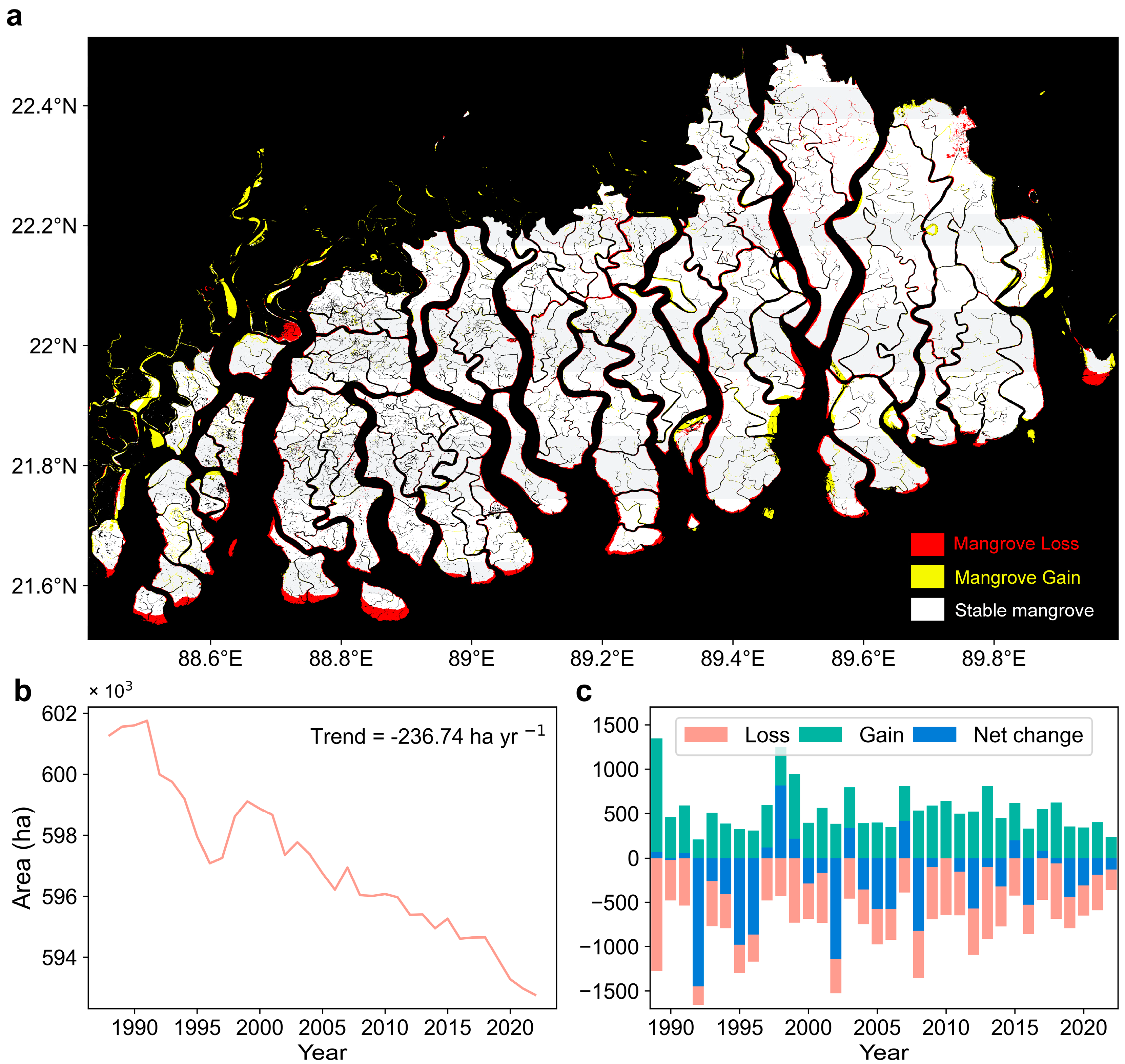
We observed both large areas of mangrove losses and gains in the Sundarbans from 1988 to 2022, with losses occurring mainly in the sea-facing parts of mangroves or along tidal creeks and gains occurring in western and eastern riverbanks (Figure 6a). Mangrove areas in the Sundarbans exhibited strong decreasing trends from 1988 to 2022, with a loss rate of 236.74 ha per year (Figure 6b), mainly due to the larger losses over gains in most years (Figure 6c). Around 27,009.79 ha of mangroves were lost, and 18,501.89 ha were gained in the Sundarbans, indicating a net mangrove loss of 8507.9 ha. Annual gains in mangrove forests were generally uniform during the period, except for two large increases in 1989 and 1998 (Figure 6c). In contrast, annual losses in mangrove areas were highly dynamic, with the most intensive net losses from 1992–1996 (Figure 6c).
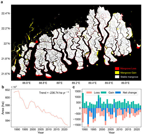
Figure 6.
The pattern of the Sundarbans mangrove changes from 1988 to 2022. (a) The mangrove change map. (b) Change in total mangrove areas over time. The trend was determined using the Theil–Sen slope estimator. (c) Temporal change of areas in mangrove loss/gain and net change (gain minus loss).
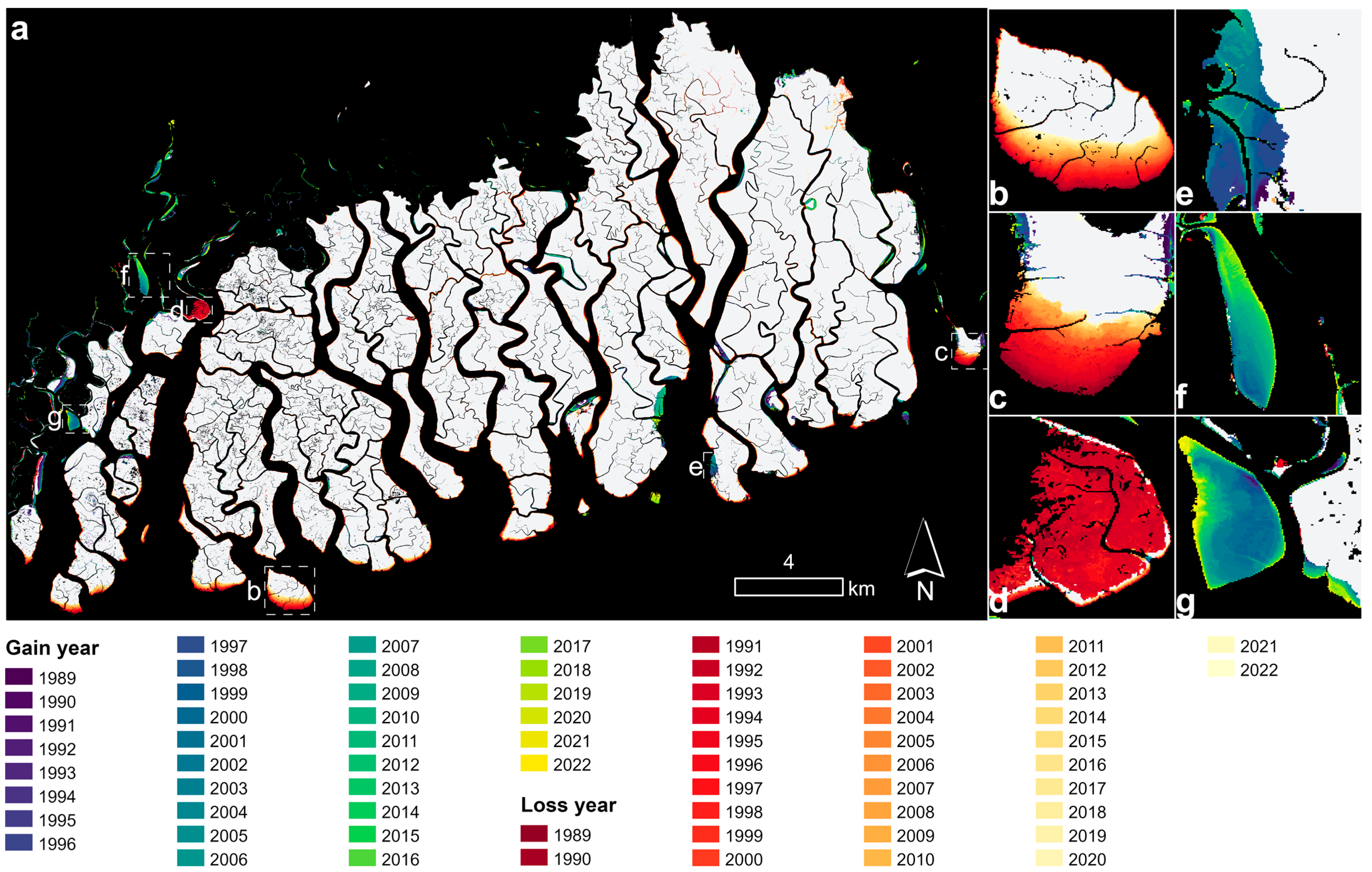
Our change map also illustrates pixel-wise timing of the loss/gain events (Figure 7a). The gradual processes of losses in sea-facing mangrove areas were accurately detected (Figure 7b,c), revealing patterns of natural erosion. In contrast, losses in land-ward mangroves tended to be abrupt, evidencing deforestation in a short period, such as 1990–1995 (Figure 7d). Gradual processes of mangrove gains along rivers were also detected. Some gains occurred around existing mangroves, reflecting the natural expansion of mangroves (Figure 7e); others did not expand from existing mangroves but instead formed large mangrove patches directly in the river (Figure 7f,g).
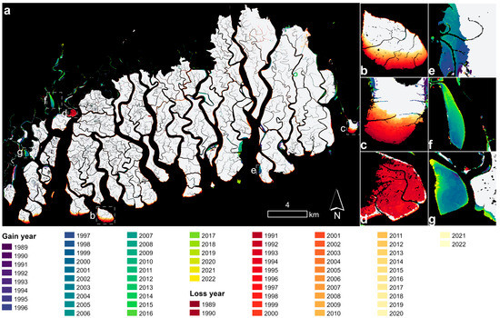
Figure 7.
(a) Spatial distribution of loss/gain timing in mangrove cover from 1988–2022. Six regional subsets of (b–d) losses and (e–g) gains show case studies of mangrove change in the Sundarbans. Note that the change map shown here delineates the last change year; that is, a single location can change more than once during 1989–2022 (1988 as the baseline), but only the latest change was indicated.
3.3. Mangrove Change Agents
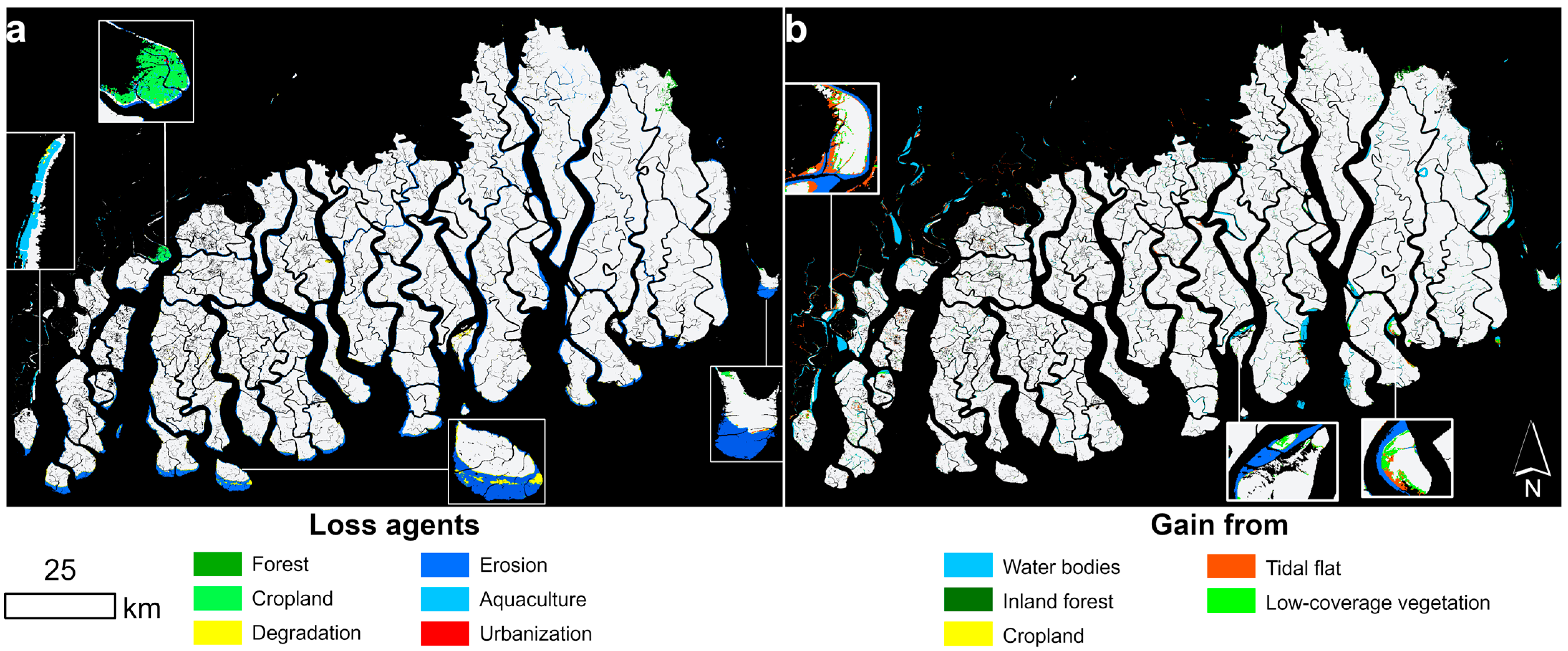
The change agent map shows notable mangrove loss/gain patterns driven by natural and anthropogenic processes (Figure 8). Erosion accounted for approximately 80.51% (21,745.10 ha) of the total mangrove loss area (27,009.79 ha) in the Sundarbans, followed by mangrove degradation accounting for 12.62% of the losses (3410.58 ha). The average erosion and degradation areas were 639.56 ha and 100.31 ha per year, respectively. Anthropogenic disturbances (i.e., aquaculture, agriculture, forest management, and urbanization) accounted for only 6.87% of the total losses, of which agricultural and aquacultural expansion were the leading causes of deforestation, with an average of 18.31 ha of mangrove loss each year. These results indicate that mangrove losses in the Sundarbans were mainly caused by natural stressors, such as sea-level rise, instead of human activities. Natural processes also dominated mangrove gains in the Sundarbans. Mangroves transferred from seawater, tidal flats, and low-coverage vegetation accounted for 65.92% (12,197.25 ha), 16.09% (2976.00 ha), and 14.95% (2766.22 ha) of the total gain area, respectively. Only 3.04% of mangroves were gained from cropland or aquaculture ponds, with an average of 8.27 ha of human-driven mangrove increase per year.
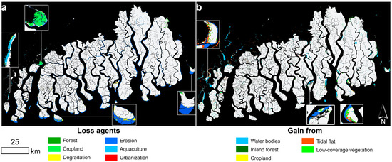
Figure 8.
Change agent maps with some regional subsets. (a) Mangrove loss agents. (b) Land-cover types from which mangroves gained.
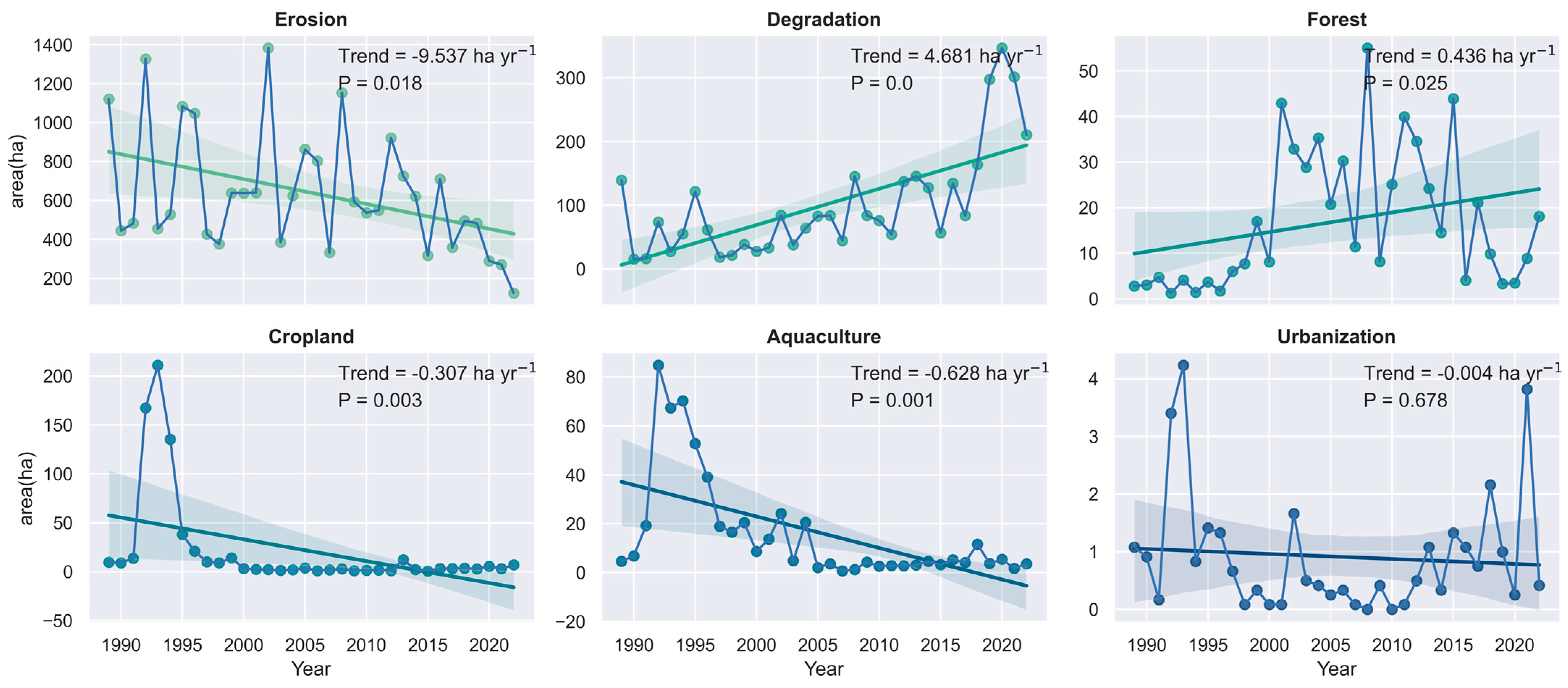
By overlaying the timing and agents of mangrove losses, we extracted the loss agent map to each year and calculated the area for each loss agent of each year to examine the temporal trend of each loss agent during 1989−2022 (1988 as the baseline) (Figure 9). While erosion was detected as the major agent of mangrove loss, we found they are significantly declining with a trend at −9.537 ha per year (Figure 9). Conversely, mangrove losses caused by degradation are increasing, with a sharp increase since 2018. Mangrove losses caused by inland forests are slightly increasing, mainly between 2000 and 2015. The losses of mangroves caused by cropland and aquaculture ponds show similar temporal trajectories, with the largest between 1990 and 2000 and declining in recent years. There was no significant trend and magnitude of mangrove losses caused by urbanization (p = 0.678), indicating that urbanization was not the main driver of mangrove losses in the Sundarbans.
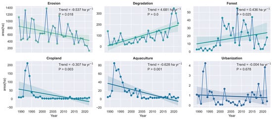
Figure 9.
Areas of six casual agents of mangrove losses at an annual step (1989–2022, 1988 as the baseline). The trend and significance were estimated using the Theil–Sen slope estimator and the Mann–Kendall trend test.
4. Discussion
4.1. Change Detection with Temporal Consistency Checking
While mangrove changes have been detected from regional to global scales, most studies focus on the accuracy of annual mangrove maps and usually have coarse temporal intervals (e.g., 5 or 10 years), lacking consideration of the temporal textual information. By combining time-series classification results and temporal information of greenness and wetness, this study detected where and when mangrove changes happened and further determined the pattern and temporal trends of change agents at the pixel level, producing 35-year annual mangrove maps in the Sundarbans with high accuracy.
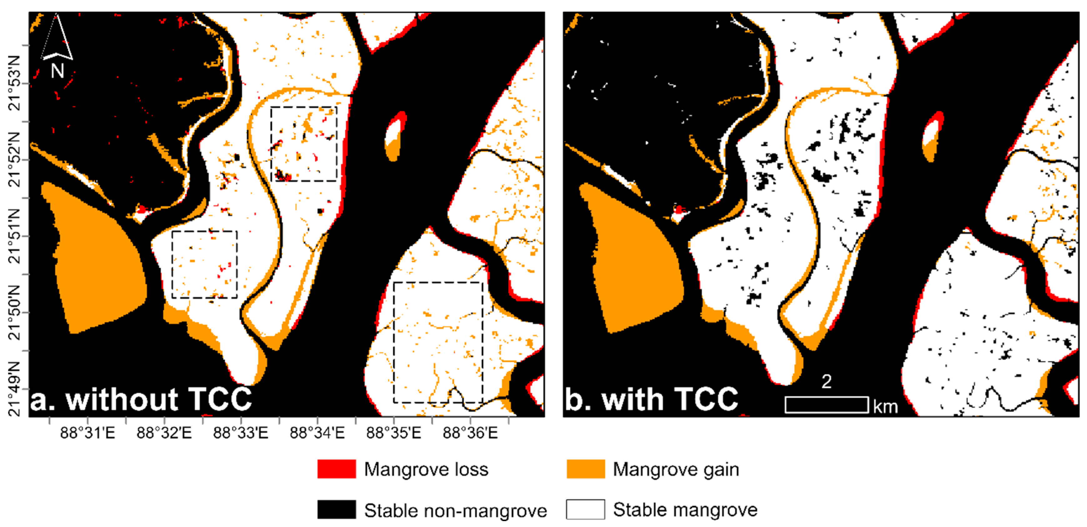
Change detection by simple classification differencing detected a lot of false changes due to classification errors in different years (Figure 10a). In contrast, TCC can improve the accuracy of change maps based on temporal textual information (Figure 10b). There are several contributions of the proposed TCC-CS approach for change detection. First, compared to previous TCC approaches [45,46], TCC-CS not only removes temporal spikes due to classification errors but also takes into account changes in greenness and wetness. Only multi-date classification differences with large deviations in greenness or wetness from mangrove samples would be considered true changes. This strategy could benefit change detection by correcting pixels that have been misclassified for consecutive years. Second, our approach can track the temporal trajectory of greenness and wetness with no need for serious calibration across sensors by using the spatial z-score. This avoids uncertainties of conventional NDVI thresholding methods [4,50] because NDVI changes can be caused by sensor replacement [51] (e.g., from Landsat TM/ETM+ to OLI) and drift [52] (e.g., MODIS). Another benefit of our approach is that mangrove changes can be detected without masking out high-tide observations. The reflectance of mangroves is highly impacted by water levels [16], and thus false changes can be detected when using images with different instantaneous tide levels. Previous approaches using high-frequency consecutive satellite observations may be invalid if consecutive high-tide observations occur. In contrast, our approach fixes the tide level to a median using annual composites, mitigating change errors caused by tidal fluctuations. Moreover, TCC-CS is computationally efficient because there is no need to fit regression lines to reconstruct spectral trajectories [53]. Given these potential advantages, the TCC-CS approach presented here allows the detection of land-cover changes in large regions.
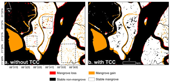
Figure 10.
Comparison of change detection results of (a) using classification differencing and (b) our temporal consistency checking approach. Dashed boxes mark some obvious classification errors.
4.2. Improvement over Existing Global Mangrove Products
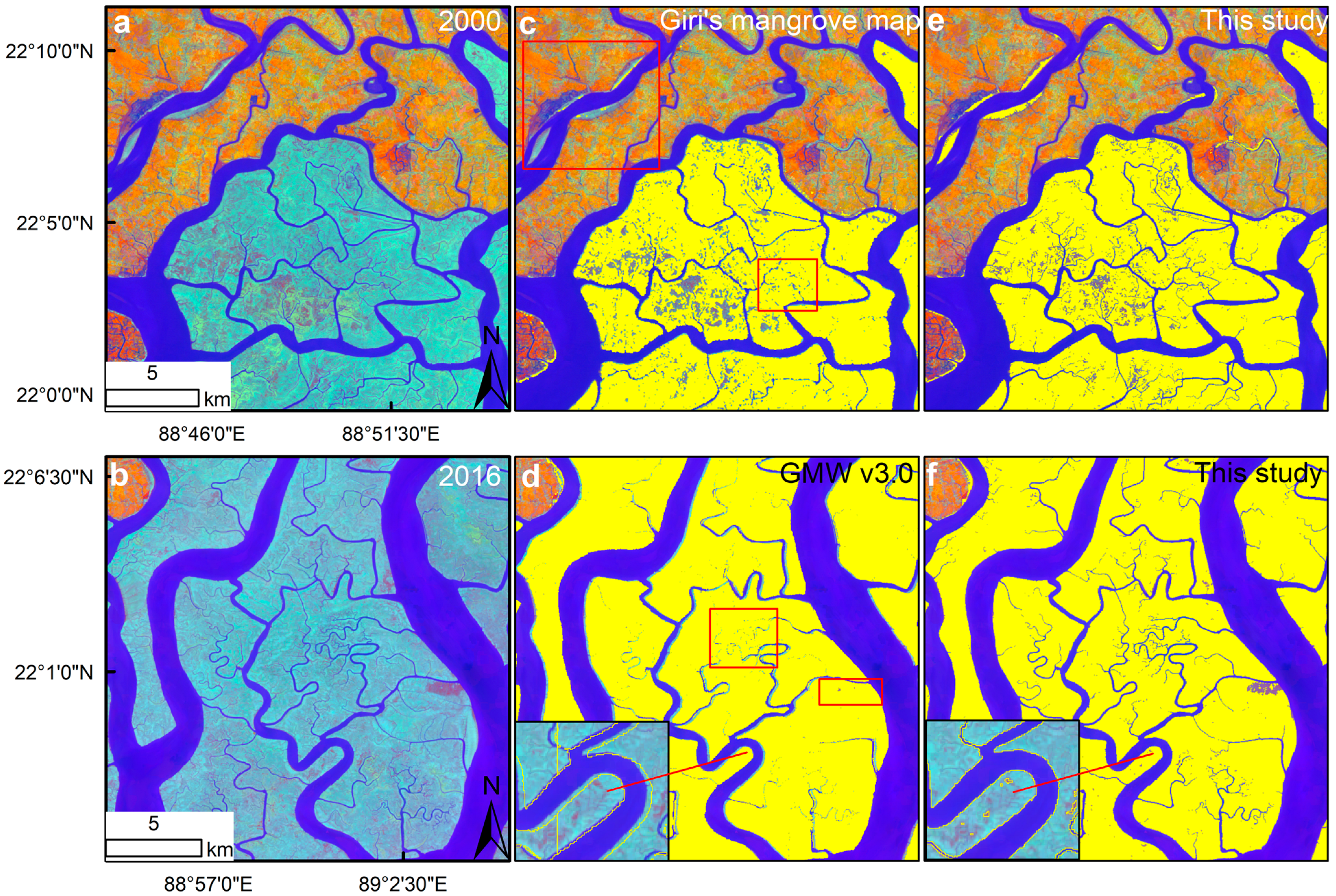
Comparing our annual mangrove maps to two widely used global mangrove products (Giri et al. [27] and GMW v3.0 [28]), we found a considerable improvement in spatial details and accuracy. We observed that Giri’s mangrove map underestimated the full extent of mangrove areas compared to this study, mainly for small riverine mangrove patches (Figure 11c). Moreover, many mangrove pixels around the canopy gaps were detected as non-mangroves by Giri’s mangrove map, thus causing more omission errors. Oppositely, mangrove areas in the GMW v3.0 contained large areas of water-dominated tidal channels and forest gaps, thus with more commission errors (Figure 11d). Moreover, mangrove patches in the GMW v3.0 cannot match the Landsat reference well (Figure 11d), mainly due to the geometric misregistration within the L-band SAR mosaics from which GMW v3.0 was generated [28]. In contrast, our annual mangrove maps contained riverine mangrove patches, accurately detected forest gaps, and reserved spatial details, such as narrow tidal channels (Figure 11e,f). These improvements are mainly due to the unmixing procedure eliminating non-vegetation-dominated pixels and the hole-filling procedure in the post-classification step.
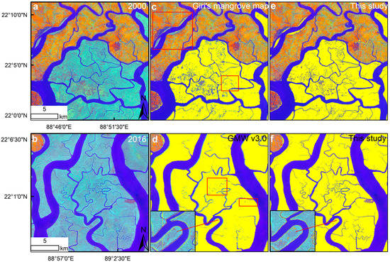
Figure 11.
Visual comparison of this study to Giri’s mangrove map in 2000 and the GMW v3.0 in 2016. The left panels (a,b) show the false-color composite of the first three components of the tasseled cap transformation (R: Brightness component; G: Greenness component; B: Wetness component). The middle panels (c,d) indicate existing mangrove maps provided by Giri et al. [27] and GMW v3.0 [28]. The red boxes mark some obvious classification errors. The inset map in (d) illustrates the mismatch between the Landsat image and GMW v3.0. The right panels (e,f) show the mangrove area detected by this study. The yellow regions represent mangrove areas.
4.3. Mangrove Losses with Sea-Level Rise
Due to their ecologically important value, the Sundarbans mangrove forests are designated as protected areas, and three wildlife sanctuaries within the Sundarbans were recognized as World Heritage Sites in 1997 [54]. Indeed, we have not detected massive mangrove logging after 1997 in the Sundarbans, which evidences the effectiveness of mangrove conservation. However, our results suggest that erosion and degradation caused extensive mangrove losses in this region, which pose new challenges for mangrove conservation. These results fit perfectly with the findings of Goldberg et al. [4] that SLR-induced erosion was the major natural cause of mangrove losses in the past decades.
SLR can cause the inundation regime (e.g., inundation depth, frequency, and duration) to exceed the physiological thresholds of mangroves and has been considered a major threat to global coastal wetland survival [55]. While mangroves can facilitate sediment deposition to defend SLR, they would still lose when the rate of SLR exceeds the capacity of mangroves to keep pace [56]. The rate of SLR in the Sundarbans is 6.04 mm per year [19], which is nearly two-folds of the global average (3.32 mm per year) [57] and is close to the threshold of 6.10 mm per year detected by Saintilan et al. [58], beyond which mangroves will be unable to sustain accretion. By increasing the pore water salinity and altering the inundation regime beyond the physiological threshold of mangroves, SLR can convert mangroves to unvegetated tidal flats (i.e., degradation) and further open water (i.e., erosion) [55]. The detected increasing/decreasing trends for erosion/degradation (Figure 9) should thus be interpreted as the time gap between degradation and submergence instead of decreasing impacts of SLR. This means the large area of mangrove degradation since 2018 (Figure 9) will convert to erosion in the next few years as SLR continues. While mangroves are resilient to SLR by landward migration and expansion with sediment accumulation [59], the total mangrove area is still declining with persistent SLR. These findings thus emphasize the importance of mitigating the magnitude of rapid SLR and ensuring sediment supply for enhancing the resilience of mangroves.
5. Conclusions
This study proposed a temporal consistency checking approach for detecting mangrove changes using a 35-year Landsat archive at the annual scale. Applying this approach to the Sundarbans, the world’s largest continuous mangrove patch, we confirmed its superior performance through both qualitative (i.e., visual comparison) and quantitative (i.e., statistical accuracy assessment) evaluation. We concluded that across the Sundarbans, from 1988 to 2022, approximately 27,009.79 ha of mangrove forests have been lost but 18,501.89 ha of mangrove have been gained, resulting in a total net loss area of 8507.9 ha. SLR-induced erosion and degradation were further identified as the main drivers of mangrove losses in the Sundarbans. Applying our temporal consistency checking approach to detect changes in mangroves and other wetland types in a larger region could be further explored in future research.
Author Contributions
Conceptualization, Z.Z., M.R.A., Y.L. (Yi Li) and Y.L. (Yangfan Li); methodology, Z.Z.; software, Z.Z.; validation, Z.Z.; writing—original draft preparation, Z.Z.; writing—review and editing, Z.Z., M.R.A., Q.Z., Y.L. (Yi Li) and Y.L. (Yangfan Li). All authors have read and agreed to the published version of the manuscript.
Funding
Y.L. (Yangfan Li) acknowledges the support from the National Natural Science Foundation of China Grants (No. 42276232), the Innovation Group Project of Southern Marine Science and Engineering Guangdong Laboratory (Zhuhai) (No. 311021004), and the Internal Program of State Key Laboratory of Marine Environmental Science (No. MELRI2205).
Data Availability Statement
The output annual mangrove maps in the Sundarbans are available here: https://figshare.com/articles/dataset/Annual_mangrove_maps_from_1988_to_2022_in_the_Sundarbans/21779636 (accessed on 25 December 2022).
Acknowledgments
The authors would like to thank all the anonymous reviewers and the editor for their constructive comments and suggestions on this manuscript.
Conflicts of Interest
The authors declare no conflict of interest.
References
- Donato, D.C.; Kauffman, J.B.; Murdiyarso, D.; Kurnianto, S.; Stidham, M.; Kanninen, M. Mangroves among the Most Carbon-Rich Forests in the Tropics. Nat. Geosci. 2011, 4, 293–297. [Google Scholar] [CrossRef]
- Lovelock, C.E.; Reef, R. Variable Impacts of Climate Change on Blue Carbon. One Earth 2020, 3, 195–211. [Google Scholar] [CrossRef]
- Regnier, P.; Resplandy, L.; Najjar, R.G.; Ciais, P. The Land-to-Ocean Loops of the Global Carbon Cycle. Nature 2022, 603, 401–410. [Google Scholar] [CrossRef]
- Goldberg, L.; Lagomasino, D.; Thomas, N.; Fatoyinbo, T. Global Declines in Human-driven Mangrove Loss. Glob. Change Biol. 2020, 26, 5844–5855. [Google Scholar] [CrossRef] [PubMed]
- Richards, D.R.; Friess, D.A. Rates and Drivers of Mangrove Deforestation in Southeast Asia, 2000–2012. Proc. Natl. Acad. Sci. USA 2016, 113, 344–349. [Google Scholar] [CrossRef]
- Hagger, V.; Worthington, T.A.; Lovelock, C.E.; Adame, M.F.; Amano, T.; Brown, B.M.; Friess, D.A.; Landis, E.; Mumby, P.J.; Morrison, T.H.; et al. Drivers of Global Mangrove Loss and Gain in Social-Ecological Systems. Nat. Commun. 2022, 13, 6373. [Google Scholar] [CrossRef]
- Hamilton, S.E.; Casey, D. Creation of a High Spatio-Temporal Resolution Global Database of Continuous Mangrove Forest Cover for the 21st Century (CGMFC-21): CGMFC-21. Global Ecol. Biogeogr. 2016, 25, 729–738. [Google Scholar] [CrossRef]
- Buelow, C.A.; Connolly, R.M.; Turschwell, M.P.; Adame, M.F.; Ahmadia, G.N.; Andradi-Brown, D.A.; Bunting, P.; Canty, S.W.J.; Dunic, J.C.; Friess, D.A.; et al. Ambitious Global Targets for Mangrove and Seagrass Recovery. Curr. Biol. 2022, 32, 1641–1649.e3. [Google Scholar] [CrossRef]
- Wang, X.; Xiao, X.; Xu, X.; Zou, Z.; Chen, B.; Qin, Y.; Zhang, X.; Dong, J.; Liu, D.; Pan, L.; et al. Rebound in China’s Coastal Wetlands Following Conservation and Restoration. Nat. Sustain. 2021, 4, 1076–1083. [Google Scholar] [CrossRef]
- Taddeo, S.; Dronova, I.; Depsky, N. Spectral Vegetation Indices of Wetland Greenness: Responses to Vegetation Structure, Composition, and Spatial Distribution. Remote Sens. Environ. 2019, 234, 111467. [Google Scholar] [CrossRef]
- Lucas, R.; Otero, V.; Van De Kerchove, R.; Lagomasino, D.; Satyanarayana, B.; Fatoyinbo, T.; Dahdouh-Guebas, F. Monitoring Matang’s Mangroves in Peninsular Malaysia through Earth Observations: A Globally Relevant Approach. Land Degrad. Dev. 2021, 32, 354–373. [Google Scholar] [CrossRef]
- Zhang, R.; Jia, M.; Wang, Z.; Zhou, Y.; Mao, D.; Ren, C.; Zhao, C.; Liu, X. Tracking Annual Dynamics of Mangrove Forests in Mangrove National Nature Reserves of China Based on Time Series Sentinel-2 Imagery during 2016–2020. Int. J. Appl. Earth Obs. Geoinf. 2022, 112, 102918. [Google Scholar] [CrossRef]
- Zhu, Z. Change Detection Using Landsat Time Series: A Review of Frequencies, Preprocessing, Algorithms, and Applications. ISPRS J. Photogramm. Remote Sens. 2017, 130, 370–384. [Google Scholar] [CrossRef]
- Lu, D.; Mausel, P.; Brondízio, E.; Moran, E. Change Detection Techniques. Int. J. Remote Sens. 2004, 25, 2365–2401. [Google Scholar] [CrossRef]
- De Jong, S.M.; Shen, Y.; de Vries, J.; Bijnaar, G.; van Maanen, B.; Augustinus, P.; Verweij, P. Mapping Mangrove Dynamics and Colonization Patterns at the Suriname Coast Using Historic Satellite Data and the LandTrendr Algorithm. Int. J. Appl. Earth Obs. Geoinf. 2021, 97, 102293. [Google Scholar] [CrossRef]
- Zhang, Z.; Xu, N.; Li, Y.; Li, Y. Sub-Continental-Scale Mapping of Tidal Wetland Composition for East Asia: A Novel Algorithm Integrating Satellite Tide-Level and Phenological Features. Remote Sens. Environ. 2022, 269, 112799. [Google Scholar] [CrossRef]
- Yang, X.; Zhu, Z.; Qiu, S.; Kroeger, K.D.; Zhu, Z.; Covington, S. Detection and Characterization of Coastal Tidal Wetland Change in the Northeastern US Using Landsat Time Series. Remote Sens. Environ. 2022, 276, 113047. [Google Scholar] [CrossRef]
- Giri, C.; Pengra, B.; Zhu, Z.; Singh, A.; Tieszen, L.L. Monitoring Mangrove Forest Dynamics of the Sundarbans in Bangladesh and India Using Multi-Temporal Satellite Data from 1973 to 2000. Estuar. Coast. Shelf Sci. 2007, 73, 91–100. [Google Scholar] [CrossRef]
- Quader, M.A.; Agrawal, S.; Kervyn, M. Multi-Decadal Land Cover Evolution in the Sundarban, the Largest Mangrove Forest in the World. Ocean. Coast. Manag. 2017, 139, 113–124. [Google Scholar] [CrossRef]
- Samanta, S.; Hazra, S.; Mondal, P.P.; Chanda, A.; Giri, S.; French, J.R.; Nicholls, R.J. Assessment and Attribution of Mangrove Forest Changes in the Indian Sundarbans from 2000 to 2020. Remote Sens. 2021, 13, 4957. [Google Scholar] [CrossRef]
- Sahana, M.; Sajjad, H.; Ahmed, R. Assessing Spatio-Temporal Health of Forest Cover Using Forest Canopy Density Model and Forest Fragmentation Approach in Sundarban Reserve Forest, India. Model. Earth Syst. Environ. 2015, 1, 49. [Google Scholar] [CrossRef]
- Rodda, S.R.; Thumaty, K.C.; Fararoda, R.; Jha, C.S.; Dadhwal, V.K. Unique Characteristics of Ecosystem CO2 Exchange in Sundarban Mangrove Forest and Their Relationship with Environmental Factors. Estuar. Coast. Shelf Sci. 2022, 267, 107764. [Google Scholar] [CrossRef]
- Mukul, S.A.; Alamgir, M.; Sohel, M.S.I.; Pert, P.L.; Herbohn, J.; Turton, S.M.; Khan, M.S.I.; Munim, S.A.; Reza, A.H.M.A.; Laurance, W.F. Combined Effects of Climate Change and Sea-Level Rise Project Dramatic Habitat Loss of the Globally Endangered Bengal Tiger in the Bangladesh Sundarbans. Sci. Total Environ. 2019, 663, 830–840. [Google Scholar] [CrossRef]
- Gorelick, N.; Hancher, M.; Dixon, M.; Ilyushchenko, S.; Thau, D.; Moore, R. Google Earth Engine: Planetary-Scale Geospatial Analysis for Everyone. Remote Sens. Environ. 2017, 202, 18–27. [Google Scholar] [CrossRef]
- Foga, S.; Scaramuzza, P.L.; Guo, S.; Zhu, Z.; Dilley, R.D.; Beckmann, T.; Schmidt, G.L.; Dwyer, J.L.; Joseph Hughes, M.; Laue, B. Cloud Detection Algorithm Comparison and Validation for Operational Landsat Data Products. Remote Sens. Environ. 2017, 194, 379–390. [Google Scholar] [CrossRef]
- Gong, P.; Liu, H.; Zhang, M.; Li, C.; Wang, J.; Huang, H.; Clinton, N.; Ji, L.; Li, W.; Bai, Y.; et al. Stable Classification with Limited Sample: Transferring a 30-m Resolution Sample Set Collected in 2015 to Mapping 10-m Resolution Global Land Cover in 2017. Sci. Bull. 2019, 64, 370–373. [Google Scholar] [CrossRef]
- Giri, C.; Ochieng, E.; Tieszen, L.L.; Zhu, Z.; Singh, A.; Loveland, T.; Masek, J.; Duke, N. Status and Distribution of Mangrove Forests of the World Using Earth Observation Satellite Data: Status and Distributions of Global Mangroves. Glob. Ecol. Biogeogr. 2011, 20, 154–159. [Google Scholar] [CrossRef]
- Bunting, P.; Rosenqvist, A.; Hilarides, L.; Lucas, R.M.; Thomas, N.; Tadono, T.; Worthington, T.A.; Spalding, M.; Murray, N.J.; Rebelo, L.-M. Global Mangrove Extent Change 1996–2020: Global Mangrove Watch Version 3.0. Remote Sens. 2022, 14, 3657. [Google Scholar] [CrossRef]
- Brandt, M.; Wigneron, J.-P.; Chave, J.; Tagesson, T.; Penuelas, J.; Ciais, P.; Rasmussen, K.; Tian, F.; Mbow, C.; Al-Yaari, A.; et al. Satellite Passive Microwaves Reveal Recent Climate-Induced Carbon Losses in African Drylands. Nat. Ecol. Evol. 2018, 2, 827–835. [Google Scholar] [CrossRef]
- Zhao, C.; Qin, C.-Z. Identifying Large-Area Mangrove Distribution Based on Remote Sensing: A Binary Classification Approach Considering Subclasses of Non-Mangroves. Int. J. Appl. Earth Obs. Geoinf. 2022, 108, 102750. [Google Scholar] [CrossRef]
- Belgiu, M.; Drăguţ, L. Random Forest in Remote Sensing: A Review of Applications and Future Directions. ISPRS J. Photogramm. Remote Sens. 2016, 114, 24–31. [Google Scholar] [CrossRef]
- Zhao, C.; Qin, C.-Z. 10-m-Resolution Mangrove Maps of China Derived from Multi-Source and Multi-Temporal Satellite Observations. ISPRS J. Photogramm. Remote Sens. 2020, 169, 389–405. [Google Scholar] [CrossRef]
- Hu, L.; Li, W.; Xu, B. Monitoring Mangrove Forest Change in China from 1990 to 2015 Using Landsat-Derived Spectral-Temporal Variability Metrics. Int. J. Appl. Earth Obs. Geoinf. 2018, 73, 88–98. [Google Scholar] [CrossRef]
- Tucker, C.J. Red and Photographic Infrared Linear Combinations for Monitoring Vegetation. Remote Sens. Environ. 1979, 8, 127–150. [Google Scholar] [CrossRef]
- Huete, A.; Didan, K.; Miura, T.; Rodriguez, E.P.; Gao, X.; Ferreira, L.G. Overview of the Radiometric and Biophysical Performance of the MODIS Vegetation Indices. Remote Sens. Environ. 2002, 83, 195–213. [Google Scholar] [CrossRef]
- Badgley, G.; Field, C.B.; Berry, J.A. Canopy Near-Infrared Reflectance and Terrestrial Photosynthesis. Sci. Adv. 2017, 3, e1602244. [Google Scholar] [CrossRef]
- Xiao, X.; Boles, S.; Frolking, S.; Salas, W.; Moore, B.; Li, C.; He, L.; Zhao, R. Observation of Flooding and Rice Transplanting of Paddy Rice Fields at the Site to Landscape Scales in China Using VEGETATION Sensor Data. Int. J. Remote Sens. 2002, 23, 3009–3022. [Google Scholar] [CrossRef]
- Baloloy, A.B.; Blanco, A.C.; Sta. Ana, R.R.C.; Nadaoka,, K. Development and Application of a New Mangrove Vegetation Index (MVI) for Rapid and Accurate Mangrove Mapping. ISPRS J. Photogramm. Remote Sens. 2020, 166, 95–117. [Google Scholar] [CrossRef]
- Diniz, C.; Cortinhas, L.; Nerino, G.; Rodrigues, J.; Sadeck, L.; Adami, M.; Souza-Filho, P. Brazilian Mangrove Status: Three Decades of Satellite Data Analysis. Remote Sens. 2019, 11, 808. [Google Scholar] [CrossRef]
- Xu, H. Modification of Normalised Difference Water Index (NDWI) to Enhance Open Water Features in Remotely Sensed Imagery. Int. J. Remote Sens. 2006, 27, 3025–3033. [Google Scholar] [CrossRef]
- Deng, Y.; Wu, C.; Li, M.; Chen, R. RNDSI: A Ratio Normalized Difference Soil Index for Remote Sensing of Urban/Suburban Environments. Int. J. Appl. Earth Obs. Geoinf. 2015, 39, 40–48. [Google Scholar] [CrossRef]
- Baig, M.H.A.; Zhang, L.; Shuai, T.; Tong, Q. Derivation of a Tasselled Cap Transformation Based on Landsat 8 At-Satellite Reflectance. Remote Sens. Lett. 2014, 5, 423–431. [Google Scholar] [CrossRef]
- Crist, E.P. A TM Tasseled Cap Equivalent Transformation for Reflectance Factor Data. Remote Sens. Environ. 1985, 17, 301–306. [Google Scholar] [CrossRef]
- Chen, B.; Xiao, X.; Li, X.; Pan, L.; Doughty, R.; Ma, J.; Dong, J.; Qin, Y.; Zhao, B.; Wu, Z.; et al. A Mangrove Forest Map of China in 2015: Analysis of Time Series Landsat 7/8 and Sentinel-1A Imagery in Google Earth Engine Cloud Computing Platform. ISPRS J. Photogramm. Remote Sens. 2017, 131, 104–120. [Google Scholar] [CrossRef]
- Li, X.; Gong, P.; Liang, L. A 30-Year (1984–2013) Record of Annual Urban Dynamics of Beijing City Derived from Landsat Data. Remote Sens. Environ. 2015, 166, 78–90. [Google Scholar] [CrossRef]
- Li, K.; Xu, E. High-Accuracy Continuous Mapping of Surface Water Dynamics Using Automatic Update of Training Samples and Temporal Consistency Modification Based on Google Earth Engine: A Case Study from Huizhou, China. ISPRS J. Photogramm. Remote Sens. 2021, 179, 66–80. [Google Scholar] [CrossRef]
- Zhu, Z.; Qiu, S.; Ye, S. Remote Sensing of Land Change: A Multifaceted Perspective. Remote Sens. Environ. 2022, 282, 113266. [Google Scholar] [CrossRef]
- Pekel, J.-F.; Cottam, A.; Gorelick, N.; Belward, A.S. High-Resolution Mapping of Global Surface Water and Its Long-Term Changes. Nature 2016, 540, 418–422. [Google Scholar] [CrossRef] [PubMed]
- Olofsson, P.; Foody, G.M.; Herold, M.; Stehman, S.V.; Woodcock, C.E.; Wulder, M.A. Good Practices for Estimating Area and Assessing Accuracy of Land Change. Remote Sens. Environ. 2014, 148, 42–57. [Google Scholar] [CrossRef]
- Campbell, A.D.; Fatoyinbo, L.; Goldberg, L.; Lagomasino, D. Global Hotspots of Salt Marsh Change and Carbon Emissions. Nature 2022, 612, 701–706. [Google Scholar] [CrossRef] [PubMed]
- Berner, L.T.; Massey, R.; Jantz, P.; Forbes, B.C.; Macias-Fauria, M.; Myers-Smith, I.; Kumpula, T.; Gauthier, G.; Andreu-Hayles, L.; Gaglioti, B.V.; et al. Summer Warming Explains Widespread but Not Uniform Greening in the Arctic Tundra Biome. Nat. Commun. 2020, 11, 4621. [Google Scholar] [CrossRef] [PubMed]
- Zhang, Y.; Song, C.; Band, L.E.; Sun, G.; Li, J. Reanalysis of Global Terrestrial Vegetation Trends from MODIS Products: Browning or Greening? Remote Sens. Environ. 2017, 191, 145–155. [Google Scholar] [CrossRef]
- Kennedy, R.E.; Yang, Z.; Cohen, W.B. Detecting Trends in Forest Disturbance and Recovery Using Yearly Landsat Time Series: 1. LandTrendr—Temporal Segmentation Algorithms. Remote Sens. Environ. 2010, 114, 2897–2910. [Google Scholar] [CrossRef]
- Islam, M.S.N. Sustainable Eco-Tourism: As a Practical Site Management Policy; A H Development Publishing House: Dhaka, Bangladesh, 2003; ISBN 978-984-8360-09-5. [Google Scholar]
- Lovelock, C.E.; Cahoon, D.R.; Friess, D.A.; Guntenspergen, G.R.; Krauss, K.W.; Reef, R.; Rogers, K.; Saunders, M.L.; Sidik, F.; Swales, A.; et al. The Vulnerability of Indo-Pacific Mangrove Forests to Sea-Level Rise. Nature 2015, 526, 559–563. [Google Scholar] [CrossRef]
- Krauss, K.W.; McKee, K.L.; Lovelock, C.E.; Cahoon, D.R.; Saintilan, N.; Reef, R.; Chen, L. How Mangrove Forests Adjust to Rising Sea Level. New Phytol. 2014, 202, 19–34. [Google Scholar] [CrossRef]
- Frederikse, T.; Landerer, F.; Caron, L.; Adhikari, S.; Parkes, D.; Humphrey, V.W.; Dangendorf, S.; Hogarth, P.; Zanna, L.; Cheng, L.; et al. The Causes of Sea-Level Rise since 1900. Nature 2020, 584, 393–397. [Google Scholar] [CrossRef]
- Saintilan, N.; Khan, N.S.; Ashe, E.; Kelleway, J.J.; Rogers, K.; Woodroffe, C.D.; Horton, B.P. Thresholds of Mangrove Survival under Rapid Sea Level Rise. Science 2020, 368, 1118–1121. [Google Scholar] [CrossRef]
- Duncan, C.; Owen, H.J.F.; Thompson, J.R.; Koldewey, H.J.; Primavera, J.H.; Pettorelli, N. Satellite Remote Sensing to Monitor Mangrove Forest Resilience and Resistance to Sea Level Rise. Methods Ecol. Evol. 2018, 9, 1837–1852. [Google Scholar] [CrossRef]
Disclaimer/Publisher’s Note: The statements, opinions and data contained in all publications are solely those of the individual author(s) and contributor(s) and not of MDPI and/or the editor(s). MDPI and/or the editor(s) disclaim responsibility for any injury to people or property resulting from any ideas, methods, instructions or products referred to in the content. |
© 2023 by the authors. Licensee MDPI, Basel, Switzerland. This article is an open access article distributed under the terms and conditions of the Creative Commons Attribution (CC BY) license (https://creativecommons.org/licenses/by/4.0/).

