Abstract
Ship instance segmentation in synthetic aperture radar (SAR) images can provide more detailed location information and shape information, which is of great significance for port ship scheduling and traffic management. However, there is little research work on SAR ship instance segmentation, and the general accuracy is low because the characteristics of target SAR ship task, such as multi-scale, ship aspect ratio, and noise interference, are not considered. In order to solve these problems, we propose an idea of scale in scale (SIS) for SAR ship instance segmentation. Its essence is to establish multi-scale modes in a single scale. In consideration of the characteristic of the targeted SAR ship instance segmentation task, SIS is equipped with four tentative modes in this paper, i.e., an input mode, a backbone mode, an RPN mode (region proposal network), and an ROI mode (region of interest). The input mode establishes multi-scale inputs in a single scale. The backbone mode enhances the ability to extract multi-scale features. The RPN mode makes bounding boxes better accord with ship aspect ratios. The ROI mode expands the receptive field. Combined with them, a SIS network (SISNet) is reported, dedicated to high-quality SAR ship instance segmentation on the basis of the prevailing Mask R-CNN framework. For Mask R-CNN, we also redesign (1) its feature pyramid network (FPN) for better small ship detection and (2) its detection head (DH) for a more refined box regression. We conduct extensive experiments to verify the effectiveness of SISNet on the open SSDD and HRSID datasets. The experimental results reveal that SISNet surpasses the other nine competitive models. Specifically, the segmentation average precision (AP) index is superior to the suboptimal model by 4.4% on SSDD and 2.5% on HRSID.
1. Introduction
Ocean ship surveillance has attracted much attention [1,2,3,4]. Compared with optical sensors [5,6,7,8], synthetic aperture radar (SAR) is more suitable for monitoring ocean ships due to its advantage of all-day and all-weather working capacity [9]. As a fundamental marine task, ship monitoring plays an important role in ocean observation, national defense security, fishery management, etc.
Traditional ship monitoring methods mainly rely on manually extracted features. For example, constant false alarm rate (CFAR) is one of the most widely used classical algorithms [10,11]. CFAR estimates the statistical data of background clutter, adaptively calculates the detection threshold, maintains a constant false alarm probability, and slides the search window to find ships. However, CFAR is sensitive to sea states, with poor migration ability. Template search is another method; still, it is hard to establish an all-round library [12,13]. Wakes can assist in seeking ships, but they do not exist widely [14]. Moreover, the above traditional methods overly rely on manual features and are time and labor consuming [15,16,17].
Recently, deep learning is offering more elegant solutions for SAR ship detection, e.g., Faster R-CNN [18], FPN [19,20,21], YOLO [22,23], SSD [24], RetinaNet [25], Libra R-CNN [26], Cascade R-CNN [27], Double-Head [28], and CenterNet [29]. So far, many scholars from the SAR community have applied them successfully to ship detection. For example, Faster R-CNN was improved by Li et al. [30], Zhang et al. [31,32], Kang et al. [33], Lin et al. [34], Deng et al. [35], and Zhao et al. [36]. Cui et al. [37], Yang et al. [38], Fu et al. [39], and Gao et al. [40] proposed various variants of FPN to boost multi-scale detection performance. YOLO was pruned by Xu et al. [41], Chen et al. [42], Zhang et al. [43,44], and Jiang et al. [45] for faster detection speed. SSD was enhanced by various tricks in the work of Wang et al. [46], Jin et al. [47], Wang et al. [48], and Zhang et al. [49]. Based on RetinaNet, Yang et al. [50] reported a false alarm suppression method; Wang et al. [51] developed an automatic ship detection system using multi-resolution Gaofen-3 images; Chen et al. [52] added a direction estimation branch for rotatable SAR ship detection; Shao et al. [53] proposed a rotated SAR ship detection method. Inspired by Libra R-CNN, Zhang et al. [54] reported a balance scene learning mechanism. Wei et al. [55] combined HR-Net [56] and Cascade R-CNN to detect ships in high-resolution SAR images. Double-Head was reflected in the work of Huang et al. [57]. Moreover, Guo et al. [58] and Cui et al. [59] used CenterNet to design more flexible networks. Additionally, Zhang et al. [60] proposed a dataset to help detect small scale ships. Still, the above works focused on ship detection at a box level (a rectangular bounding box corresponds to a ship). They did not achieve a united detection and segmentation (instance segmentation). Segmentation is in fact the most ideal paradigm to achieve ocean ship surveillance, offering the classification of ship hull and background at a pixel level, and it can provide more detailed location information and shape information. Ship instance segmentation in SAR images is of great importance for port ship scheduling and traffic management. It cannot be neglected.
Some reports attempted SAR ship semantic segmentation. Fan et al. [61] designed a fully convolutional network using U-Net [62] to classify ship, land, and sea using polarimetric SAR images, but their method cannot distinguish different ships; thus, the number of ships is not available. From the perspective of computer vision (CV), they only achieved semantic segmentation rather than instance segmentation. We refer readers to Ref [63] for their similarities and differences. Zhang et al. [64] improved HTC to realize SAR ship instance segmentation, but their network is big and has many false alarms. Li et al. [65] improved U-Net further using a 3D dilated multi-scale mechanism. Jin et al. [66] proposed one patch-to-pixel convolutional neural network (CNN) for PolSAR ship detection. They achieved a ship–background binary classification, but many land pixels were misjudged as ships. This is because their method does not have the ability to distinguish land pixels.
Several public reports that have conducted SAR ship instance segmentation are from Su et al. [67] and Wei et al. [68], according to our survey in Ref [69]. Su et al. [67] designed a HQ-ISNet (a HR-SDNet’s extension [55]) for remote-sensing image instance segmentation. They have evaluated HQ-ISNet using optical and SAR images but have not considered the characteristic of the targeted SAR ship task, e.g., ship aspect ratio, cross sidelobe, speckle noise, etc. Only generic tricks were offered (generic vs. targeted), still with great obstacles, to further improve accuracy. Wei et al. [68] released a high-resolution SAR images dataset (HRSID), which is the first open dataset for SAR ship instance segmentation. HRSID offered research benchmarks using generic instance segmentation models from the CV community, e.g., Mask R-CNN [70], Mask Scoring R-CNN [71], Cascade Mask R-CNN [72], and hybrid task cascade (HTC) [73,74], but no methodological contributions were offered for scholars to learn from.
In view of the characteristics of the SAR ship instance segmentation task, we conduct related research. Inspired by network in network (NIN) [75], which establishes micro subnetworks in a network, we report an idea of scale in scale (SIS), which establishes multi-scale modes in a single scale. For the targeted SAR ship task, we tentatively equip SIS with four types of modes, i.e., the input mode, backbone mode, RPN mode, and ROI mode. More modes can be included in the future.
The input mode establishes an image pyramid at the network input end to handle cross-scale ship detection (large size differences [76]). The backbone mode establishes multiple hierarchical residual-like connections in a single layer to extract multi-scale features with increased receptive fields at the granular level [77]. The RPN mode adopts multiple asymmetric convolutions to replace vanilla single square convolutions. This can generate proposals that are more consistent with ship aspect ratios. The ROI mode adds multi-level background contextual information of ROIs to ease the adverse effects of speckle noise, cross sidelobe, and ship blurring edges, which can suppress pixel false alarms in mask prediction. Combining them, a SIS network (SISNet) is proposed for high-quality SAR ship instance segmentation based on the mainstream two-stage Mask R-CNN framework [70]. The results indicate that each mode offers an observable accuracy gain.
We also report two extra improvements on Mask R-CNN. (1) FPN is redesigned. One content-aware reassembly of features (CARAFE) module [78] is recommended to generate an extra bottom level to boost small ship detection. One bottom-up path aggregation (PA) branch is added to shorten the pyramid information path using more accurate localization signals existing in low levels [79] conducive to stable training and large ship positioning. (2) The detection head (DH) is redesigned via a cascaded triple structure for a more refined box regression to enable better mask prediction. The results verify each improvement’s effectiveness.
The results on SSDD [69] and HRSID [68] indicate that SISNet surpasses the other nine competitive methods. (1) Compared with the vanilla Mask R-CNN, SIS-Net improves the detection average precision (AP) by 9.9% and 5.4% on SSDD and HRSID, respectively, and pushes the segmentation AP by 7.3% and 4.1% on SSDD and HRSID, respectively. (2) Compared with the existing best model, its detection AP superiority is 5.1% and 3.3% on SSDD and HRSID, respectively; its segmentation AP superiority is 4.4% and 2.5% on SSDD and HRSID, respectively.
Ultimately, based on Faster R-CNN with FPN [18,19], four modes are extended to a pure detection task. The results show their universal effectiveness, with an observable accuracy gain.
The main contributions of this paper are as follows.
- A SISNet is proposed, delving into high-quality SAR ship instance segmentation based on Mask R-CNN.
- In SISNet, four SIS modes, i.e., the input mode, backbone mode, RPN mode, and ROI mode, are proposed. In SISNet, two additional improvements, i.e., redesigned FPN and redesigned DH, are proposed.
- To verify the effectiveness of SISNet, we conduct extensive experiments on public dataset SSDD and HRSID. SISNet offers a state-of-the-art performance.
2. Methodology
Figure 1 is Mask R-CNN’s framework. Mask R-CNN is Faster R-CNN’s extended version. By contrast, it adds a mask prediction branch to its DH. The proposals from RPN are mapped into the backbone to extract ROI features twice. One extraction is for classification and regression, and the other is for segmentation. ROIAlign was used to replace ROIPool [80] to remove misalignments between the ROIs and extracted features. FPN [19] was applied to Mask R-CNN for better multi-scale segmentation. Mask R-CNN refers to its FPN version in this paper. Mask R-CNN is a main-stream two-stage instance segmentation framework in the CV community, so it is selected. We refer readers to Ref [70] for more details.
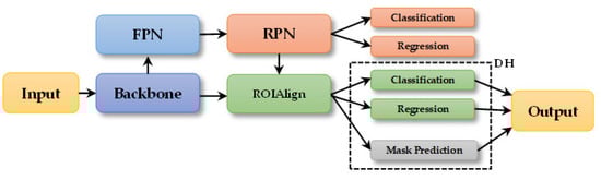
Figure 1.
Architecture of Mask R-CNN.
Based on Mask R-CNN, we propose SISNet. As shown in Figure 2, we embodied the input mode, backbone mode, RPN mode, and ROI mode in the input, backbone, RPN, and ROIAlign (marked by  in Figure 2). Additionally, we redesigned FPN and DH (marked by
  in Figure 2). As shown in Figure 2, the input SAR images are first sent into the input mode to obtain multi-scale inputs. Then, the multi-scale inputs are sent into the backbone mode to extract multi-scale features with gradually increased receptive fields at the granular level. Next, the output features are sent into redesigned FPN for feature fusion enhancement. The output features of redesigned FPN and the output features of the backbone mode are sent into the RPN mode and ROIAlign mode. Finally, the outputs of the ROIAlign mode are sent into redesigned DH to obtain the SAR ship instance segmentation results. Additionally, Table 1 is the architecture diagram of SISNet.
in Figure 2). Additionally, we redesigned FPN and DH (marked by in Figure 2). As shown in Figure 2, the input SAR images are first sent into the input mode to obtain multi-scale inputs. Then, the multi-scale inputs are sent into the backbone mode to extract multi-scale features with gradually increased receptive fields at the granular level. Next, the output features are sent into redesigned FPN for feature fusion enhancement. The output features of redesigned FPN and the output features of the backbone mode are sent into the RPN mode and ROIAlign mode. Finally, the outputs of the ROIAlign mode are sent into redesigned DH to obtain the SAR ship instance segmentation results. Additionally, Table 1 is the architecture diagram of SISNet.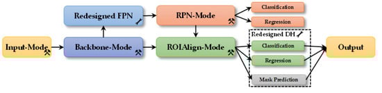
Figure 2.
Architecture of SISNet. means four SIS modes. means two improvements.
means four SIS modes. means two improvements.

Table 1.
Architecture diagram of SISNet.
2.1. Input Mode
The input mode can be counted as a multi-scale training test [81]; it is yet endowed with a new idea, i.e., establishing multi-scale inputs in a single scale. It can solve cross-scale detection (targets have a large pixel scale difference [76]). The large scale difference is often due to the large resolution difference [82,83]. Figure 3 is the input mode’s sketch map. Figure 4 represents the cross-scale ships in SSDD.
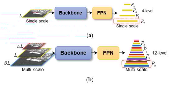
Figure 3.
Input mode. (a) Single scale. (b) Multi scale.
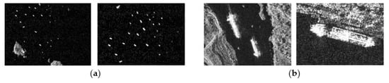
Figure 4.
Cross-scale ships. (a) Small ships. (b) Large ships.
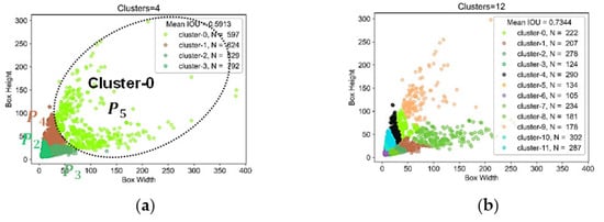
If the single scale is L in Figure 3a, then the raw FPN scales are L/4, L/8, L/16, and L/32 in P2, P3, P4, and P5; therefore, four levels are used for multi-scale detection. Yet, using four levels, it is still difficult to perform cross-scale detection, according to the K-means clustering results in Figure 5a. For example, P5 should be responsible for detecting large ships in Cluster-0, but the scale difference is too large in Cluster-0 (loose distribution). With the input mode, the input scales are αL, L, and βL in Figure 3b. The sequence 0 < α < 1 is used to improve the regression of large ships (i.e., shrinking), and β > 1 is used to detect smaller ships (i.e., stretching). The 3-level image pyramid equivalently sets up a 12-level feature pyramid (4 × 3). Intuitively, 12 levels should be better than the 4 ones from the mean intersection over union (IOU) [84] in Figure 5 (0.7344 > 0.5913). Note that the equivalent 12-level FPN is in fact virtual and has the same parameter quantity as the 4-level one. One can up- or down-sample the 4-level FPN to build a real 12-level one, but this must increase the parameters and calculation costs. We set L, α, β to [512, 0.8125, 1.1875] on SSDD empirically. They are [1000, 0.80, 1.20] on HRSID. We set three scales for accuracy–speed trade-offs. More scales might obtain better accuracy but must sacrifice speed. In Section 5, we will conduct experiments to study the impact of input scales on accuracy and speed.
2.2. Backbone Mode
The backbone mode will establish multiple hierarchical residual-like connections among a single 3 × 3 convolution (conv) layer to extract multi-scale features with gradually increased receptive fields at the granular level [77]. It is used in the backbone. Figure 6 is its sketch map. We use ResNet-101 [85] as the baseline.
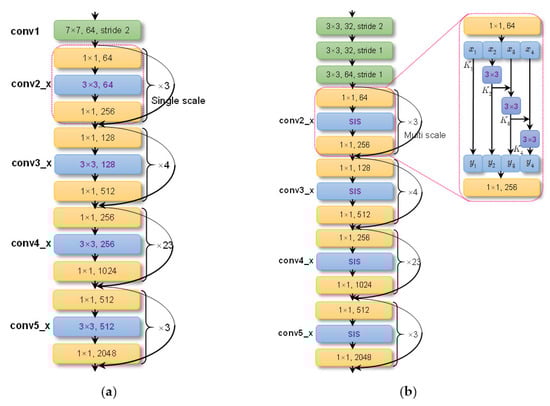
Figure 6.
Backbone mode. (a) ResNet-101. (b) ResNet-101-SIS.
In Figure 5, the conv2_x to conv5_x are bottleneck blocks, sharing a similar structure, i.e., 1 × 1 conv for channel reduction, 3 × 3 conv for feature extraction, and 1 × 1 conv for channel increase. The features are extracted by a 3 × 3 conv in a layer-wise manner, with limited receptive fields. Now, we replace the single-scale 3 × 3 conv with four smaller groups of filters (x1, x2, x3, and x4). Each subset xi has the same spatial size but 1/4 channel number (see the enlarged region in Figure 6b). Each subset is treated by each different branch (K1, K2, K3, and K4) in a divide-and-conquer way, making the network more efficient [86]. The number of smaller groups of filters is set to four, similar to ResNext [75]. Different from ResNeXt [87] and Inception [88], we connect the different filter groups in a hierarchical residual-like manner to increase the range of receptive fields progressively using three 3 × 3 convs. The above can be described by
Each 3 × 3 conv Ki() can potentially receive information from all feature subsets {xj, j ≤ i}. After a subset xj passes through a 3 × 3 conv, the output has a larger receptive field than xj. For combinatorial explosion effects, the final output contains different numbers and combinations of receptive field sizes or scales [77]. We call the above backbone-mode SIS. It can be seen from a single-scale layer to multi-scale ones or from a single-scale receptive field to multi-scale ones (1 → 3). The output of a bottleneck block changes to their concatenation [y1, y2, y3, y4].
Moreover, different from Ref [77], the top 7 × 7 conv is replaced with three 3 × 3 convs (equivalent to a 27 × 27 conv). This can further enlarge receptive fields without increasing the parameters.
2.3. RPN Mode
The RPN mode is inspired by the ship label aspect ratio distribution, as in Figure 7. Here, the ship length and breadth are not identified. In Figure 7, the labels of ships often have large aspect ratios (1365 >> 325, 1222 >> 325). The symmetrical funnel-shaped size distribution in Figure 5 also confirms this case. One can take advantage of this prior to preset the anchors. Yet, using square convs to extract non-square features might still destroy the coupling relationship between the length direction and breadth one. This was also revealed by Han et al. [89].
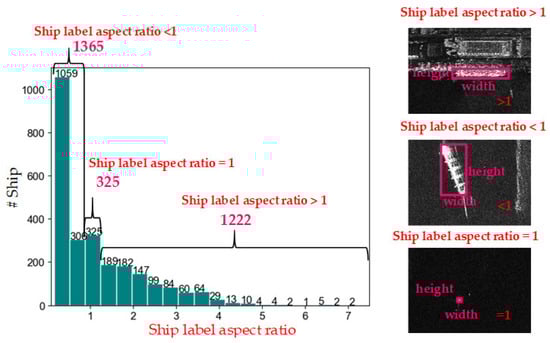
Figure 7.
Ship label aspect ratio (label box width/label box height) distribution in SSDD. Note that ship length and breadth are not identified.
Thus, the RPN mode uses multi-asymmetric convs to replace the single square conv to generate proposals, which are more in line with ship aspect ratios. The RPN mode is a shift from a single-scale conv to multi-scale/shape convs. Here, the scale refers specifically to ship label aspect ratio. Figure 8 is its sketch map, where k = 3 is the number of anchors, similar to FPN. We add a 1 × 3 conv and a 3 × 1 conv. To retain the detection performance of square ships (mostly small ships with few pixels), the raw 3 × 3 conv is still reserved. Their outputs are concatenated. To balance the contributions (1365 vs. 325 vs. 1222), a global context block (GCB) [90] is used to model channel correlation. The above is described by
Z and Z′ are the input and output, and fGCB is the GCB operator.
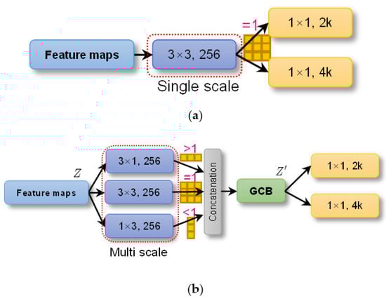
Figure 8.
RPN mode. (a) Single square conv. (b) Multi-asymmetric convs.
Figure 9 is GCB’s implementation. C is the channel number; H and W denote spatial sizes. GCB has a context modeling module and a transform one. The former adopts 1 × 1 conv Wk and softmax to generate attention weights A and conducts global attention pooling to obtain the global context features (from C × H × W to C × 1 × 1). This is equivalent to the global average pooling (GAP) [75] in squeeze and excitation (SE) [91], but the average form is replaced by an adaptive attention weighted form. The latter is similar to SE, but before the rectified linear unit (ReLU), the output of the 1 × 1 squeeze conv Wv1 is normalized to enable better generalization, equivalent to the regularization of batch normalization (BN) [92]. To refine the more salient features of three parallel differently shaped convs, the squeeze ratio r is set to 3. The last 1 × 1 conv Wv2 is used to transform the bottleneck to capture channel-wise dependencies. The element-wise addition is used for feature fusion. The above is described by
where xi is the input of GCB, zi is the output, is global attention weights, Wv2ReLU is the bottleneck transform, LN is the layer normalization, and Np = HW is the entire space. In short, GCB can capture long-range dependencies via aggregating the query-specific global context to each query position [90] with the feature self-attention function of non-local networks [93]. The resulting output Z’ is able to better balance the contributions of different conv branches in Figure 8b, making proposals better accord with ship aspect ratios.
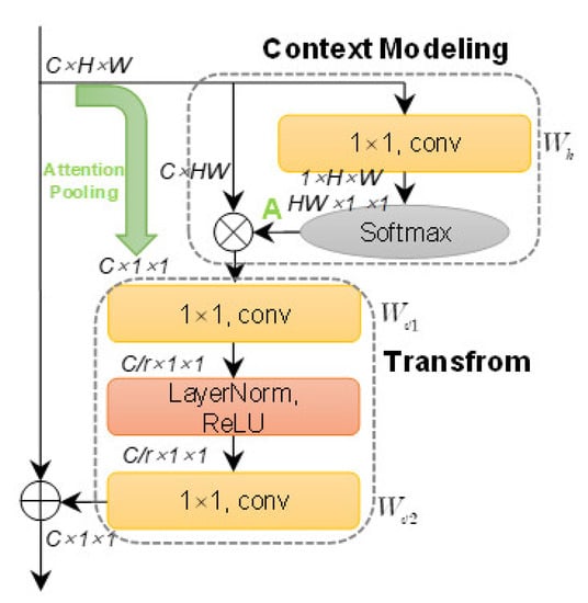
Figure 9.
Global context block (GCB).
2.4. ROI Mode
The ROI mode is inspired by specific SAR imaging mechanisms. Figure 10 shows ships with speckle noise, cross-sidelobe, wakes, and unclear edges. The detection bounding box can tightly frame a ship, but it reduces the receptive fields of the subsequent segmentation task [94,95]. This makes it impossible to observe more ship backgrounds, e.g., ship-like pixel noise and ship wakes. The box can eliminate the cross-sidelobe deviating too far from the ship center, but few sidelobe and noise pixels in the box make it difficult to ensure a segmentation network’s learning benefits. Ship edges are also unclear [96], so it is necessary to expand the receptive field to explicitly find the boundary between a ship and its surrounding. Yet, the receptive field provided by the detection box cannot enable the segmentation network to observe the entire ship surrounding and its edge. In short, the above cases due to specific SAR imaging mechanisms pose challenges for follow-up background–ship pixel binary classification. Thus, the ROI mode adds multi-level background contextual information to ease the adverse effects from speckle noise, cross-sidelobe, wakes, and unclear edges to suppress pixel false alarms during mask prediction.
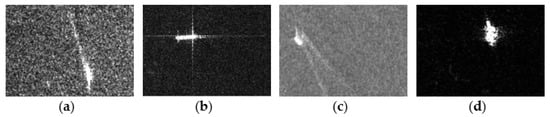
Figure 10.
Various ships in SAR images. (a) Speckle noise. (b) Cross-sidelobe. (c) Wakes. (d) Unclear edges.
Figure 11 is its sketch map. The ROIAlign output size for box classification and regression is 7 × 7; meanwhile, that for mask prediction is 14 × 14, similar to Mask R-CNN. The latter requires more spatial information to ensure segmentation performance.
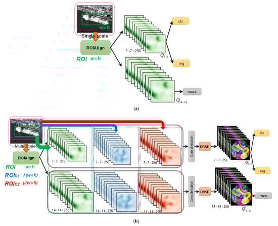
Figure 11.
ROI-mode SIS. (a) Single-scale ROI. (b) Multi-scale ROIs. cls: classification. reg: regression. mask: mask prediction.
For the ROI with a (w × h) size, the ROI mode adds two-level context information, denoted by ROIC1 with a λ(w × h) size marked in blue in Figure 11b and ROIC1 with a μ(w × h) size marked in red in Figure 11b, respectively. We only add two extra contextual ROIs considering a trade-off between accuracy and speed. λ > 1 and μ > 1 mean enlarging the ROI to receive external surrounding context information. λ is set to 2, and μ is set to 3, empirically. Note that Kang et al. [33] also added context information, but multi-level contexts were not considered. The ROIAlign outputs of three-level ROIs are concatenated directly. To avoid possible training oscillation due to injecting too many irrelevant backgrounds, we use SE to refine the features and then apply a feature dimension reduction (256 × 3→256), i.e., suppressing useless information and highlighting valuable one. We modify the raw SE to make it possess the function of dimension reduction (DR). The modified version is named DRSE. DRSE not only reduces the computational burden on the backend but also ensures a seamless connection to the follow-up box classification regression and mask prediction branches, avoiding troublesome interface designs. To sum up, the above is described by
where fDRSE is the DRSE operator, and Q’ is the output. The 7 × 7 spatial size Q’ is used for box classification and regression, and the 14 × 14 one is used for mask prediction.
Figure 12 is DRSE’s implementation. In the collateral branch, GAP is used to obtain global spatial information; 1 × 1 conv and the sigmoid function are used to squeeze the channels to focus on important ones. The squeeze ratio p is set to 3 (256 × 3→256). In the main branch, the input channel number is reduced directly using a 1 × 1 conv and ReLU. The broadcast element-wise multiplication is used for compressed channel weighting. DRSE models the channel correlation of input feature maps in a reduced dimension space. It uses the learned weights from the reduced dimension space to pay attention to the important features of the main branch. It avoids the potential information loss of the rude dimension reduction. In short, the above is described by
where X is the input, Y is the output, σ is the sigmoid function, and ⊙ denotes the broadcast element-wise multiplication.
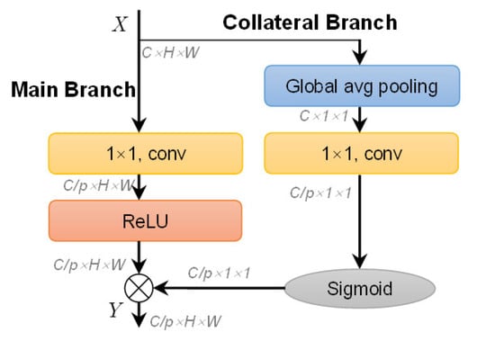
Figure 12.
Dimension reduction squeeze and excitation (DRSE).
2.5. Redesigned FPN
We redesign the FPN, so as to enhance small ship detection. Figure 13 shows the raw FPN and the redesigned one. C2, C3, C4, and C5 are the outputs of conv2_x, conv3_x, conv4_x, and conv5_x in Figure 6. If the input size is L, then their sizes are L/4, L/8, L/16, and L/32. C1 is not used because the top is a 1 × 1 conv rather than a bottleneck block. Abandoning C1 can also reduce computational burdens [19]. A top-down branch is designed to transmit high-level strong semantic information to the bottom by up-sampling. This can improve the pyramid’s representation [19]. To obtain a larger anchor scale, P6 is set via applying a stride@2 max pooling of P5 [19]. The raw FPN is described by
where UpSa×2 is the ×2 up-sampling, and MaxPool×2 is the ×2 max pooling. Five levels are used for multi-scale detection and segmentation (P2, P3, P4, P5, and P6). Yet, the SAR ships are often very small for the characteristics of the “bird’s-eye” view of SAR. This is different from most natural optical images with the “person’s-eye” view. Although network deepening can enable stronger semantic features, small ships are progressively diluted due to their faint spatial features, declining their detection and segmentation performance, so many small ships are missed.
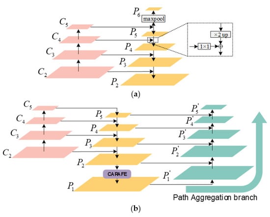
Figure 13.
FPN. (a) The raw FPN in Mask R-CNN. (b) The redesigned FPN.
CARAFE. We add an extra bottom level (P1) for better small ship detection. Its size is L/2. P1 can be obtained by × 2 up-sampling or × 2 deconvolution, but we recommend CARAFE [78]. This is because (1) unlike × 2 up-sampling by bilinear interpolation, which focuses on subpixel neighborhoods, CARAFE offers a large field of view, which can aggregate contextual information; (2) unlike deconvolution, which uses a fixed kernel for all samples, CARAFE can enable instance-specific content-aware handling, which can generate adaptive kernels on the fly [78].
Different from Ref [78], which used CARAFE to replace all × 2 up-sampling layers (P5 → P4, P4 → P3, P3 → P2), CARAFE is only used to generate the extra bottom-level P1 (P2 →P1) considering the trade-off between speed and accuracy. We find that the raw top-level (P6) does not play a big role; thus, to reduce computing costs, it is deleted. Figure 14 is CARAFE’s implementation. CARAFE contains a kernel prediction process and a feature reassembly one. The former is used to predict an adaptive × 2 up-sampling kernel Kl’ corresponding to the l’ location of feature maps after up-sampling from the original l location. The kernel size is kup × kup, which means kup × kup neighbors of the location l. kup is set to 5 empirically, same as the raw report in Ref [78]. That is, CARAFE can consider the surrounding 5 pixels for up-sampling interpolation (5 × 5 = 25 pixels in total). The weights of these 25 pixels are obtained by adaptive learning. In the kernel prediction process, one 1 × 1 conv is used to compress the channel to refine the salient features, where the compression ratio d is set to 4, i.e., the raw 256 channels are compressed to 64. This can not only reduce the calculation amount but also ensure the benefits of the predicted kernels [82]. One 3 × 3 conv is used to encode contents whose channel number is k2up × 22, where 2 denotes the up-sampling ratio (H→2H, W→2W). The dimension transformation is completed by the pixel shuffle operation [97]. Then, each reassembly kernel is normalized by a softmax function spatially to reflect the weight of each sub-content. Finally, the learned kernel Kl’ serves as the kernel of the follow-up feature reassembly process. The feature reassembly is a simple kup × kup conv. We refer readers to Ref [78] for more details.
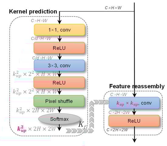
Figure 14.
Content-aware reassembly of features (CARAFE).
PA. We find that the initial redesigned FPN (P1, P2, P3, P4, P5) sacrifices the detection performance of large ships to a certain extent, especially the large ships loosely distributed in Figure 5. This may be due to the removal of P6. Moreover, it also leads to occasional training instability, possibly due to the extremely unbalanced proposal numbers in each pyramid level. This may arise from too many proposals of the added P1 level. Thus, inspired by PANet [79], an extra bottom-up path aggregation (PA) branch is designed to handle the above problems. This branch transmits accurate localization signals existing in low levels to the top again, so as to make up for lost spatial information. This makes the positioning of large ships more accurate, so as to avoid missed detections. With the top-down branch and the bottom-up one, the feature pyramid information path is greatly shortened, which speeds up the information flow. A network with faster information flow speed can integrate the features of each level comprehensively and produce some mutual restraints, so as to avoid falling into the local optimization of a certain level. Finally, more stable training can be achieved. Additionally, this PA branch can also, in fact, enhance segmentation performance further because refined spatial information in low levels can be captured emphatically. This is also revealed by Liu et al. [79]. In short, the above can be described by
where P’i denotes the output of the PA branch.
2.6. Redesigned DH
We redesign DH in Mask R-CNN via a cascaded triple structure for a more refined box regression, inspired by Refs [27,28]. “Triple structure” refers to three parallel branches (a box classification branch, a box regression one, and a mask prediction one). “Cascaded” means that multiple triple structures are connected successively in a cascade. In this way, high-quality boxes can be achieved to enable better mask prediction. The box quality is generally evaluated using the IOU with the corresponding ground truth (GT) [84], as in Figure 15. If the IOU threshold is 0.5 (the PASCAL VOC criterion [98]), Box A and Box B can both detect the ship successfully, but obviously, Box B is better. In particular, the mask prediction of Box B is more accurate than that of Box A. Figure 16 shows the raw DH and the redesigned one.
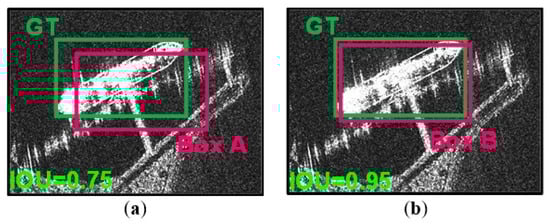
Figure 15.
Prediction box. (a) IOU = 0.75. (b) IOU = 0.95.
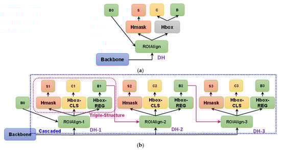
Figure 16.
Detection head (DH). (a) The raw DH in Mask R-CNN. (b) The redesigned DH. B0 denotes the box regression of RPN. B denotes the box regression. C denotes the box classification. S denotes the mask prediction.
Triple Structure. In Figure 16a, the raw box classification (C) and regression (B) share the same branch (Hbox), which contains two fully connected (FC) layers in Mask R-CNN. Yet, this is not conducive to box regression because FC layers offer less spatial positioning information than conv ones. In fact, FC is more suitable for classification due to its strong semantic information, whereas conv is more suitable for regression due to its strong space location information [28]. Thence, we split the raw Hbox into two different parallel branches (Hbox-CLS and Hbox-REG). Each branch will bear its own responsibility to give full play to their respective advantages. In this way, classification and regression are divided and ruled efficiently. The above is known as double head by Wu et al. [28]. Hbox-CLS remains the same as Hbox, but the number of FC layers is halved to reduce computing costs. We find that too many FC layers bring an almost unobservable accuracy gain because the classification task is too simple (ship–background binary classification), and it is not as difficult as generic object detection in the CV community, e.g., the classification tasks on 21 categories of targets in PASCAL VOC [98] and 81 categories of targets in COCO [99]. This is consistent with the previous report of Ref [100]. Hbox-REG contains four conv layers and a GAP for the final regression. The number of conv layers is set to four empirically, same as the number of conv layers in the Hmask [28]. Finally, one detection head will be equipped with three parallel branches (Hbox-CLS, Hbox-REG, and Hmask). We call it a triple structure.
Cascaded. Three triple structures are cascaded successively via connecting the front-end box regressor (B1 → ROIAlign-2 and B2 → ROIAlign-3). Each DH is trained sequentially with increasing IOU thresholds (0.50 → 0.60 → 0.70) by using the output of the front-end DH as the training set for the next. We only set three stages (DH-1, DH-2, and DH-3) considering the trade-off between accuracy and speed. More stages might achieve better performance, but the resulting added parameters slow down the training. Higher IOU threshold at the backend can improve box positioning precision further. Moreover, such progressive resampling can also improve the hypotheses’ quality, guaranteeing a positive training set of equivalent size for all heads and minimizing overfitting [27]. As a result, the terminal B3 will become tighter than B2 and B1, which can enable more superior mask prediction. Note that the ROI-mode SIS introduced in Section 2 D is only applied to ROIAlign-1 (the input end of the whole DH) because DH should better be injected with modest contextual information; otherwise, too much contextual information existing in the backends (e.g., ROIAlign-3) potentially makes the training unstable. In fact, the above cascaded concept is inspired by Cascade R-CNN [27], but Cascade R-CNN belongs to a double structure rather than our triple structure.
3. Experiments
3.1. Dataset
SSDD and HRSID are the two unique open datasets for SAR ship instance segmentation. SSDD is the first open dataset for SAR ship detection, which was released by Li et al. [30] in 2017. Its official release version [69] offers instance segmentation labels. SSDD has 1160 SAR images from RadarSat-2, TerraSAR-X, and Sentinel-1. The polarizations are HH, VV, VH, and HV. The resolutions range from 1 m to 10 m. The test set has 232 samples with the filename suffix of 1 and 9. The remaining samples constitute the training set. HRSID is the first open SAR ship instance dataset, which was released by Wei et al. [68] in 2020. It has 5604 SAR images from Sentinel-1 and TerraSAR-X. The polarizations are HH, HV, and VV. The resolutions are 0.5 m, 1 m, and 3 m. The training set has 3642 samples. The test set has 1962 samples.
3.2. Experimental Detail
We use stochastic gradient descent (SGD) to train SISNet in 12 epochs. The learning rate is 0.002, which is reduced by 10 times at 8 epochs and 11 epochs. The momentum is 0.9, and the weight decay is 0.0001. The batch size is 1 due to limited GPU memory. We use the pretrained weights on ImageNet to fine-tune the network. The classification loss Lcls is cross-entropy [101], and the regression one Lreg is smooth L1 [73], same as Mask R-CNN. The total multi-task learning loss function is defined by
means the type i loss of type j task; wDH-1, wDH-2, and wDH-3 are the loss weights of DH-1, DH-2, and DH-3. They are set to 1, 0.50, and 0.25, respectively, same as Cascade R-CNN. The larger weight of DH-1 can punish its lower IOU threshold to avoid too many false positive samples being input to the terminal DH and vice versa for DH-3. The base anchor size is 8. The anchor ratios are 0.5, 1.0, and 2.0, and the strides are 2, 4, 8, 16, and 32. Due to the added P1/ level, the feature map stride list of ROIAlign is changed to [2, 4, 8, 16, 32], corresponding to , , , , and . The random sampling ratio of positive and negative samples is 1:3. The IOU threshold of positive and negative samples is 0.50 in DH-1, 0.60 in DH-2, and 0.70 in DH-3, as mentioned in Section 2 F. The IOU threshold of positive samples is 0.70 in RPN, and that of negative samples is 0.30, same as Mask R-CNN.
The image pyramid of the input mode is constructed by bilinear interpolation. The default input size in SSDD is [416, 512, 608] because images in SSDD have an average size of 512 × 512, and another two settings are inspired by YOLOv3 [102]. Thus, the baseline size in SSDD is 512. The default input size in HRSID is [800, 1000, 1200], so the baseline in HRSID is 1000, similar to Ref [68]. Data augmentation is not used because the input-mode SIS expands the number of samples to three times the raw number. By inference, non-maximum suppression (NMS) [103] is used to delete duplicate boxes with an IOU threshold of 0.50. Other configurations without special instructions are the same as the vanilla Mask R-CNN. Other models for performance comparison are trained on SAR datasets again, with their pretrained weights on ImageNet under basically the same hyperparameters as in our SISNet. We try to remain as consistent as possible with their original reports to re-implement their models. The experiments are run on a personal computer (PC) with RTX3090 GPU and i9-10900 CPU. The software framework is mmdet [104] based on Pytorch.
3.3. Evaluation Criteria
The COCO metrics [99] are adopted. Their core index is the average precision (AP), that is, the average value of precisions under ten IOU thresholds from 0.50 to 0.95 with an interval of 0.05. AP50 denotes the average precision under an IOU threshold of 0.50. AP75 denotes that under an IOU threshold of 0.75. APS denotes the average precision of small ships (<322 pixels). APM denotes that of medium ships (>322 pixels and <962 pixels). APL denotes that of large ships (>962 pixels). The above metrics cover the detection task and the segmentation one.
Additionally, we use FPS to measure the detection speed. FPS represents the number of images the network can process per second. The larger the FPS, the faster the network segmentation speed. In addition, we measure network complexity by the number of parameters (#Para) the network contains. The bigger #Para, the more complex the network.
4. Results
4.1. Quantitative Results
Table 2.
Quantitative results on SSDD. Blue “+X.X” denotes the accuracy gain on the baseline. magenta “+X.X” denotes the accuracy advantage against the suboptimal method. The suboptimal method is marked by underline “—”.
Table 3.
Quantitative results on HRSID. Blue “+X.X” denotes the accuracy gain on the baseline. magenta “+X.X” denotes the accuracy advantage against the suboptimal method. The suboptimal method is marked by underline “—”.
Baseline. Mask R-CNN is our baseline. It is reproduced by us basically keeping it the same as its raw report. Its detection and segmentation AP are comparable to existing reports [68, 106], even better. Thus, our baseline is credible and persuasive.
Models for Comparison. We reproduce the other nine models for performance comparison as basically the same as their raw reports. Mask Scoring R-CNN [71] added a mask scoring branch. Cascade Mask R-CNN [72] is an implementation based on Cascade R-CNN. HTC [73] added a mask communication branch based on Cascade Mask R-CNN. PANet [79] added a path aggregation branch to boost the information flow. YOLACT [94] is a one-stage instance segmentation model. GRoIE [105] redesigned the region of interest extraction layer. HQ-ISNet [67] applied the HR-Net [56] for remote-sensing image instance segmentation, which achieved SAR ship instance segmentation. SA R-CNN was reported by Zhao et al. [106] two months ago, where synergistic attention was presented to improve SAR ship segmentation performance. The above models are trained on SAR ship images again using basically the same training strategies, so their re-implementations are credible and persuasive. Taking HTC as an example, our reproduced detection AP is 66.6%, and the segmentation AP is 55.2% on HRSID; these are comparable to the re-implementations of Zhao et al. [106]. Furthermore, their re-produced HTC accuracies (65.1% detection AP and 54.2% segmentation AP) are slightly poorer than ours, which may be due to our more appropriate training strategies. Since the input-mode SIS is equivalent to the multi-scale training test, we train and test most other models in a multi-scale manner, again, for comparison fairness (marked by †).
- Each technique (redesigned FPN, redesigned DH, and four SIS modes) is useful. The accuracy gradually increases with the progressive insertion of each technique to the baseline. This shows the correctness of the theoretical analysis in Section 2. The detection AP is improved by 9.9% on SSDD and by 5.4% on HRSID. The segmentation AP is improved by 7.3% on SSDD and by 4.1% on HRSID. Certainly, the detection speed is expectedly sacrificed. The accuracy–speed trade-off is a permanent topic, which will be considered in the future.
- The accuracy gains of different techniques are differentiated, but each of them is always instrumental in performance improvements, more or less. Thus, the accuracy still exhibits an upward trend. Each technique accuracy sensitivity upon the whole SISNet will be introduced in Section 5 in the form of each installation and removal.
- The detection accuracies are universally higher than the segmentation ones, regardless of SSDD and HRSID, because the latter is more challenging and detects ships at the pixel level.
- The accuracies on HRSID are universally lower than those on SSDD because HRSID have more complex SAR images, so more efforts should be made on HRSID in the future.
- SISNet surpasses the other competitive models dramatically. The suboptimal model is from HTC [73]. Still, its detection performance is lower than SISNet by 5.1% on SSDD and by 3.3% on HRSID. Its segmentation performance is still lower than SISNet by 4.4% on SSDD and by 2.5% on HRSID. This fully shows the state-of-the-art performance of SISNet.
- The detection speed of SISNet is inferior to others, but it offers more accuracy gains. This shortcoming needs to be handled in the future. Despite this, SISNet is still better than others because when only three techniques (the redesigned FPN, the redesigned DH, and the input SIS mode) are used, the performance of SISNet outperforms the others already. That is, the detection AP on SSDD is 67.7%, which is already better than that of HTC by 0.9% (66.8%). The segmentation AP on SSDD is 61.4%, which is already better than that of HTC by 0.7% (60.7%). Meanwhile, in the above case, the detection speed of SISNet is 3.31 FPS, which is comparable to others to some degree.
- YOLACT offers the fastest detection speed, since it is a one-stage model, but its accuracy is too poor to meet the application requirements. Its performance is greatly lower than SISNet’s, i.e., on SSDD, its detection is 54.0% AP << SISNet’s detection 71.9% AP, and its segmentation is 48.4% AP << SISNet’s segmentation 65.1% AP. The same is true on HRSID.
- SISNet’s model size is 909 MB, and its parameter quantity is 118.10 M. This seems to be acceptable due to the fact that the model size of HTC reaches 733 MB, and HQ-ISNet has 98.79 M parameters. Therefore, although SISNet has the highest complexity, its high accuracy makes up for it, which is worth it. The segmentation performance of SISNet is higher than HTC by 4.4% on SSDD and by 2.5% on HRSID. Thus, SISNet may still be cost effective.
Figure 17 presents the loss curves on the training set and validation set of SSDD and HRSID. As can be seen in Figure 17, SISNet can converge rapidly through the loss function we use. As shown in Figure 17a, SISNet converges after about 8 epochs on SSDD. As shown in Figure 17b, SISNet converges after about 9 epochs on the more complex HRSID dataset. In addition, on both SSDD and HRSID, the gap between training loss and validation loss is narrow, which proves that the overfitting phenomenon does not appear. If there is an overfitting phenomenon, the validation loss will suddenly increase, but this phenomenon does not occur in Figure 17.
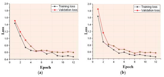
Figure 17.
Loss curve of SISNet. (a) SSDD. (b) HRSID.
4.2. Qualitative Results
Figure 18 and Figure 19 present the quantitative results on SSDD and HRSID. The IOU threshold is 0.50. FN is the number of false negatives (missed detections); FP is that of false positives (false alarms). SISNet is compared with the suboptimal HTC due to limited space.
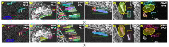
Figure 18.
Qualitative results on SSDD. (a) The suboptimal HTC. (b) SISNet. Ground truths are marked by green boxes. False alarms are marked by orange boxes.
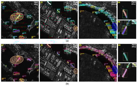
Figure 19.
Qualitative results on HRSID. (a) The suboptimal HTC. (b) SISNet. Ground truths are marked by green boxes. False alarms are marked by orange boxes.
- SISNet offers a higher detection rate than HTC (see the blue ellipse regions). In the #1 image of Figure 18, HTC missed a ship, while SISNet detected it smoothly. In the #3 image of Figure 19, HTC missed three ones parked at ports, while SISNet missed one. The same is true on other images. This benefits from the combined action of the proposed improvements.
- SISNet offers a lower false alarm rate than HTC (see the orange ellipse regions). In the #1 image of Figure 19, HTC generated four false alarms, whereas SISNet generated one. In the #2 image of Figure 19, HTC generated one false alarm, whereas SISNet suppressed it. The same is true on other images. This is because SISNet can receive more background context information via the adopted ROI-mode SIS, boosting its foreground–background discrimination capacity.
- SISNet offers better detection performance of small ships. In the #6 image of Figure 18, eleven small ships were missed by HTC, whereas SISNet detected three of them. This is because our redesigned FPN can ease the spatial feature loss of small ships. Now, SAR small ship detection is a challenging topic due to fewer features, but SISNet can deal with this task well.
- SISNet offers better detection performance of large ships. In the #4 image of Figure 18, the positioning accuracy of HTC was poorer than that of SISNet. Moreover, HTC resulted in two extra false alarms arising from repeated detections. The same situation also occurred on the #4 and #5 images of Figure 19. The redesigned DH and the PA branch in the redesigned FPN both play a vital role in detecting large ships. The multi-cascaded regressors of the former can progressively refine the positioning of large ships. More spatial location information is transmitted to the pyramid top by the latter, which can improve the representativeness of high-level features.
- SISNet offers better detection performance of densely parallel parked ships. In the #3 image of Figure 18, although the ship hulls overlap, SISNet can still detect them and then segment them. However, HTC misses most of them. At present, densely parallel parked ship detection is a challenging topic for mutual interferences, but SISNet can handle this task well.
- SISNet offers better detection performance of inshore ships. In all inshore scenes, SISNet detected more ships than HTC; meanwhile, it still avoided more false alarms. Now, inshore ship detection is a challenging topic because of more complex backgrounds and serious interferences of landing ship-like facilities, but SISNet can deal with this task well.
- SISNet offers more credible detection results (see the yellow ellipse regions). In the #5 image of Figure 18, the box confidence of HTC is 0.99, which is still lower than that of SISNet (1.0). In the #6 image of Figure 18, the box confidences of three small ships are all inferior to that of SISNet (i.e., 0.74 < 0.87, 0.70 < 0.98, and 0.96 < 0.99). This is because the triple structure of the redesigned DH can decouple the classification and regression task, enabling superior classification performance. Thus, SISNet enables more high-quality SAR ship detection.
- SISNet offers better segmentation performance. In the #4 image of Figure 18, the total pixels of the ship were separated into three independent regions by HTC, but this case did not occur on SISNet. In the #6 image of Figure 18, some scattered island pixels were misjudged as ship ones by HTC, but this case also did not occur on SISNet. This is because the ROI-mode SIS can enable the network to observe more surroundings to suppress pixel false alarms.
- SISNet offers superb multi-scale/cross-scale detection–segmentation performance. Regardless of very small ships or rather large ones, SISNet can always detect them. This benefits from the multi-scale image pyramid of the input-mode SIS, the more robust feature extraction of the backbone-mode SIS, the optimized proposals of the RPN-mode SIS, and the more robust multi-level features of the redesigned FPN.
- In short, SISNet offers state-of-the-art SAR ship instance segmentation performance.
5. Ablation Study
In this section, we will carry out extensive ablation studies to confirm the effectiveness of each contribution and to determine some vital hyperparameters. Moreover, we also offer some potential suggestions to boost the current SISNet’s instance segmentation performance further. Experiments are performed on SSDD. When discussing a certain improvement technique, for rigorous comparative experiments, we freeze the other five and then install and remove this certain improvement technique.
5.1. Ablation Study on Input Mode
(1) Effectiveness of Input Mode.Table 4 shows the quantitative results with/without the input-mode SIS. As shown in Table 4, the input-mode SIS enables a 3.1% detection AP gain. The segmentation AP gain also reaches up to 3.1%, which shows its effectiveness. Multi-scale performance is improved due to the obvious increases in APS, APM, and APL. This is because cross-scale ships can be detected more easily by the multi-level image pyramid constructed. Finally, the combination of the image and feature pyramid enables superior multi-scale instance segmentation performance. Certainly, the input-mode SIS is not free, which reduces the detection speed from 4.46 FPS to 1.84 FPS. One can reduce the scale number for accuracy–speed trade-offs.
Table 4.
Quantitative results with and without input-mode SIS.
(2) Different Input Sizes. In this experiment, we discuss the effect of input sizes on accuracy, complexity, and speed. Table 5 shows the quantitative results with different input sizes. We discuss the single-scale, double-scale, triple-scale, and quad-scale cases. Although multi-scale training and testing is common, this issue has not been surveyed comprehensively in the SAR community. As shown in Table 5, the accuracy becomes better with more scales, but the speed is reduced. One can set large input sizes to further improve performance, e.g., the double-scale combination of [608, 704], i.e., 72.7% detection AP and 66.1% segmentation AP. Still, one must consider the GPU memory’s upper limitation because training larger images requires more memory. It is also related to expense costs because larger memory GPUs are more expensive. Additionally, input sizes do not affect the number of parameters of SISNet, so the model complexity is not affected by the number of input sizes.
Table 5.
Quantitative results with different input sizes in SISNet.
(3) Larger Input Sizes.Table 6 shows the quantitative results with larger input sizes. We only study the single-scale case. As shown in Table 6, a larger input size enables better performance, but there is a saturation value, e.g., the detection AP reaches the peak 71.9%. Segmentation is more sensitive to sizes than detection because it operates at the pixel level. Larger size is beneficial for suppressing pixel-level false alarms. Thus, detection and segmentation are imbalanced. One must treat them differently, e.g., designing a weighted loss function and a task-decoupling network.
Table 6.
Quantitative results with larger input sizes in SISNet.
5.2. Ablation Study on Backbone Mode
(1) Effectiveness of Backbone Mode. Table 7 shows the quantitative results with/without backbone-mode SIS. One can observe that backbone-mode SIS improves the detection AP by 1.2% and segmentation AP by 1.7%. This benefits from more representative multi-scale ship features extracted from the proposed ResNet-101-SIS, where a series of small group filters can extract both local and global features, and the multiple hierarchical residual-like connections can fuse them effectively to enable efficient information flow. As a result, the instance segmentation performance can be improved. Moreover, if one sets more conv filters and adds more residual-like connections in Figure 6b, the performance may become better, but this must result in larger computational load. This requires reasonable trade-offs.
Table 7.
Quantitative results with and without backbone-mode SIS.
(2) Compared with Other Backbones. We compare ResNet-101-SIS with other backbones in Table 8. As shown in Table 8, ResNet-101-SIS offers the best segmentation AP compared to others, although its detection AP is slightly lower than ResNeXt-101-64x4d-DCN [107], RegNetX-4.0GF [108], and HRNetV2-W40 [56]. Despite all this, we think our ResNet-101-SIS should still be cost effective. Taking ResNeXt-101-64x4d-DCN as an example, it does offer the optimal 72.4% detection AP, but its speed is inferior to our ResNet-101-SIS (1.12 FPS < 1.84 FPS); moreover, its model size reaches up to 2.57 GB, which is greatly heavier than 909 MB ResNet-101-SIS. ResNet-101-SIS is also superior to Res2Net-101 because the top larger receptive field enables better segmentation performance. Because of the better performance of ResNeXt-101-64x4d-DCN compared to ResNeXt-101-64x4d (72.4% detection AP > 71.4% detection AP), one might apply deformable convs to ResNet-101-SIS for better accuracy in the future, but the speed–accuracy trade-offs need consideration.
Table 8.
Quantitative results with different backbones in SISNet.
5.3. Ablation Study on RPN Mode
(1) Effectiveness of RPN Mode. Table 9 shows the quantitative results with/without the RPN-mode SIS. As shown in Table 9, RPN-mode SIS improves the detection AP by 0.9%; the segmentation AP gain is 1.1%, showing its effectiveness. This is because the multiple asymmetric convs used in RPN-mode SIS can model ship shapes effectively, ensuring better proposals. In Table 9, the superscript * means that one 3 × 3 square conv is used in Figure 8a. Superscript † means that one 3 × 3 square conv, one 3 × 1 asymmetric conv, and one 1 × 3 asymmetric conv are used in Figure 8b.
Table 9.
Quantitative results with and without RPN-mode SIS.
(2) Different Convs and GCB. We discuss the different conv combinations and GCB in Table 10, using multiple asymmetric convs can mostly improve detection accuracy, but the segmentation accuracy seems to become slightly poor, to some degree. This might arise from their imbalanced contribution allocation. However, once GCB is embedded, the segmentation AP is improved obviously. More reasons need to be studied deeply in the future. Therefore, when using RPN-mode SIS, GCB is an indispensable tool; otherwise, the performance would develop in the opposite direction of expectation. In Table 10, the superscript * means that the inputs of 3 × 3, 3 × 1, and 1 × 3 convs are concatenated directly. Superscript † means that the concatenated inputs of 3 × 3, 3 × 1, and 1 × 3 convs are refined by a 3 × 3 conv. Superscript ◆ means that the concatenated inputs of 3 × 3, 3 × 1, and 1 × 3 convs are refined by GCB in Figure 8b.
Table 10.
Quantitative results of different convs and GCB in RPN-mode SIS.
5.4. Ablation Study on ROI Mode
(1) Effectiveness of ROI Mode. Table 11 shows the quantitative results with/without ROI-mode SIS. As shown in Table 11, ROI-mode SIS boosts the detection AP by 1.4% and the segmentation AP by 2.0%. Thus, injecting contextual information into ROIs is helpful for SAR ship detection and segmentation. Contextual information can help the network better observe ship surroundings, which can make the learning of background features more effective, so as to ease their interferences. Our experimental results are also in line with Kang et al. [33]. By contrast, we proposed using multi-scale ROIs, but Kang et al. [33] only used the single-scale larger ROI. In Table 11, the superscript * represents single-scale ROI in Figure 4a. Superscript † represents multi-scale ROI in Figure 11b.
Table 11.
Quantitative results with and without ROI-mode SIS.
(2) Different ROIs and DRSE. We discuss the different ROIs and DRSE in the ROI-mode SIS, as shown in Table 12. As shown in Table 12, more ROIs with larger context ranges could mostly offer better performance. The double ROIs perform better than the single ROI. When triple ROIs are used, one should balance their contribution allocation reasonably; otherwise, the performance does not always improve. Therefore, DRSE is used in SISNet. DRSE can boost the segmentation AP strongly from 63.45% to 65.1%. In Table 12, the superscript * represents single-scale ROI in Figure 11a. Superscript † represents multi-scale ROI in Figure 11b. Superscript 1 represents the raw w × h ROI. Superscript 2 represents the added 2(w × h) ROI, i.e., λ = 2.0, in Figure 11b. Superscript 3 represents the added 3(w × h) ROI, i.e., μ = 3.0, in Figure 11b.
Table 12.
Quantitative results of different ROIs and DRSE in ROI-mode SIS.
(3) Different Range Contexts. We determine the amplification factor λ and μ through experiments in Table 13. As shown in Table 13, the combination of [1.0, 2.0, 3.5] enables the optimal detection AP, but it is far inferior to that of [1.0, 2.0, 3.0] in terms of the segmentation AP (64.3% < 65.1%). Thus, in the ROI-mode SIS, [1.0, 2.0, 3.0] is selected. Moreover, a larger amplification factor consumes more time, which requires a trade-off.
Table 13.
Quantitative results of different range contexts in ROI-mode SIS.
(4) More ROIs. We use more ROIs to explore their influences on performance in Table 14, where we arrange another two ROIs that are denoted by ROIC1f and ROIC1b, whose amplification factors are set to 1.5 and 2.5. As shown in Table 14, this practice does not bring notable performance improvements, but the speed is further reduced. The small intervals between the amplification factors lead to redundancy of each other’s backgrounds. In Table 14, the subscript C1f denotes the front of C1. C1b denotes the rear of C1.
Table 14.
Quantitative results of more ROIs in ROI-mode SIS.
(5) Shrinking ROIs. Furthermore, it is an interesting idea whether one can shrink ROIs to achieve performance improvements. We conduct an extra experiment regarding this, where λ and μ are set to 0.7 and 0.5, respectively. The results are shown in Table 15. As shown in Table 15, the above practice is infeasible. The detection–segmentation performances are both reduced greatly. This may be because the terminal regressor can more easily shrink the detection box according to the enlarged ROI feature learning.
Table 15.
Quantitative results of shrinking ROIs in ROI-mode SIS.
5.5. Ablation Study on Redesigned FPN
(1) Effectiveness of Redesigned FPN. Table 16 shows the quantitative results with and without the redesigned FPN. In Table 16, the superscript * represents the raw FPN in Figure 13a. Superscript * represents the redesigned FPN in Figure 13b. As shown in Table 16, the redesigned FPN is superior to the raw FPN by 2.2% detection AP and 2.4% segmentation AP. The detection APS is boosted by 2.6%, and the segmentation APS is boosted by 2.3%. This benefits from the added P1 level, which can retain small ship spatial features and avoid the feature loss among the pyramid top. Moreover, the detection APL is boosted by 5.8%, but the segmentation APL is reduced to 62.5%. This might be due to the removal of P6. Yet, the added PA branch can make up for such loss because spatial information is transmitted to the pyramid top again to enhance the representation of high levels.
Table 16.
Quantitative results with and without redesigned FPN SIS.
(2) Component Analysis of Redesigned FPN. We analyze the different components in the redesigned FPN in Table 17. In Table 17, the superscript * means that one simple up-sampling layer with bilinear interpolation is used to replace CARAFE in Figure 13b. Superscript ◆ means that one deconvolution layer is used to replace CARAFE in Figure 12b. Superscript † means that CARAFE is used in Figure 13b. In Table 17, one can find that (i) P1 can boost small ship instance segmentation, e.g., the detection APS is improved from 69.1% to 71.3%. (ii) P6 is helpful for large ship instance segmentation while reducing the inference speed. When P6 is deleted, the large ship instance segmentation performance is indeed reduced. (iii) PA can compensate for the large ship accuracy loss (48.0% → 57.9%). The resulting accuracy is even better than the raw case with P6 (57.9% > 56.3%), so adding PA and deleting P6 is better. (iv) CARAFE offers better performance than bilinear interpolation up-sampling because it enables instance-specific content-aware handling, generating adaptive kernels on the fly, which can boost the representation of the pyramid bottom level. (v) Deconvolution does not improve the performance as expected but reduces it. We find that it leads to instability in training. This might be because deconvolution to the too-large-sized feature maps P1 easily causes an “uneven overlap”, putting more of the metaphorical paint in some places than others [111]. More possible reasons need to be studied further in the future.
Table 17.
Quantitative results of different components in redesigned FPN.
(3) Compared with Other FPNs. We also compare the redesigned FPN with other FPN architectures in Table 18. In Table 18, SS-FPN [110] and Quad-FPN [82] are proposed for targeted SAR ship detection, whereas the other five [19,26,56,78,79] are proposed for generic object detection in the CV community. As shown in Table 18, our redesigned FPN has the best performance compared to others. The sub-optimal competitor is Quad-FPN, but its segmentation AP is still far lower than ours (63.5% < 65.1%); moreover, its inference speed is slower than ours. This fully reveals our redesigned FPN’s superiority.
Table 18.
Quantitative results of different FPNs.
5.6. Ablation Study on Redesigned DH
(1) Effectiveness of Redesigned DH. Table 19 shows the quantitative results with and without the redesigned DH. As shown in Table 19, our redesigned DH improves the detection AP by 4.0% and the segmentation AP by 3.4%, showing its effectiveness. In the redesigned DH, the triple structure can decouple classification and regression using different branches. Each branch will bear its own responsibility to give full play to their respective advantages. In this way, classification and regression are divided and ruled efficiently. Moreover, the cascaded manner can improve positioning performance gradually.
Table 19.
Quantitative results with and without redesigned DH.
(2) Component Analysis of Redesigned DH. We analyze the different components in the redesigned DH in Table 20. In Table 20, one can clearly observe that the triple structure and the cascaded manner can both boost instance segmentation performance. It should be noted that Wu et al. [22] directly demonstrated the effectiveness of the double structure, and Cai et al. [20] directly confirmed the effectiveness of the cascaded manner. In essence, our redesigned DH is a straightforward and intuitive combination of the two, which has not been reported previously.
Table 20.
Quantitative results of different components in redesigned DH.
6. Discussion
Last but not least, we also discuss the universal effectiveness of the proposed four SIS modes and two improvements. We extend them to the pure detection task based on the popular Faster R-CNN with FPN [18,19]. The results are shown in Table 21. As shown in Table 21, each proposed technique is effective for SAR ship detection, with the gradual increase in detection AP, i.e., 62.5% → 65.4% → 66.1% → 67.1% → 68.3% → 68.6% → 70.3%. Thence, this work is credible and persuasive.
Table 21.
Extension to detection task based on Faster R-CNN.
7. Conclusions
Ship instance segmentation in SAR images is of great importance for port ship scheduling and traffic management. At present, there are few research works on SAR ship instance segmentation. Furthermore, multi-scales, different aspect ratios of ships, and noise interference hinder the improvement of accuracy. In order to solve these problems, we propose a SIS idea for SAR ship instance segmentation. Based on Mask R-CNN, we propose a SISNet, which is equipped with four modes, i.e., the input mode, backbone mode, RPN mode, and ROI mode. We redesign the FPN and DH of raw Mask R-CNN to further improve performance. The results on open datasets show that SISNet surpasses the other nine state-of-the-art models. We perform ablation studies to confirm the effectiveness of the four modes and two improvements. The four modes and two improvements are extended to a pure detection task based on Faster R-CNN. The results can reveal their universal effectiveness.
Author Contributions
Conceptualization, Z.S.; methodology, Z.S.; software, Z.S.; validation, Z.S.; formal analysis, Z.S.; investigation, Z.S.; resources, Z.S.; data curation, Z.S.; writing—original draft preparation, Z.S.; writing—review and editing, X.Z. (Xu Zhan) and T.Z. (Tianwen Zhang); visualization, S.W., J.S. and X.X.; supervision, X.K., T.Z. (Tianjiao Zeng) and X.Z. (Xiaoling Zhang); project administration, X.Z. (Xiaoling Zhang); funding acquisition, X.Z. (Xiaoling Zhang). All authors have read and agreed to the published version of the manuscript.
Funding
This work was supported by the National Natural Science Foundation of China (61571099).
Data Availability Statement
Not applicable.
Acknowledgments
We would like to thank all editors and reviewers for their valuable comments for improving this manuscript.
Conflicts of Interest
The authors declare no conflict of interest.
References
- Zhang, T.; Zhang, X.; Shi, J. HyperLi-Net: A hyper-light deep learning network for high-accurate and high-speed ship detection from synthetic aperture radar imagery. ISPRS J. Photogramm. Remote Sens. 2020, 167, 123–153. [Google Scholar] [CrossRef]
- Xu, X.; Zhang, X.; Shao, Z.; Shi, J.; Wei, S.; Zhang, T.; Zeng, T. A Group-Wise Feature Enhancement-and-Fusion Network with Dual-Polarization Feature Enrichment for SAR Ship Detection. Remote Sens. 2022, 14, 5276. [Google Scholar] [CrossRef]
- Zhang, T.; Zeng, T.; Zhang, X. Synthetic Aperture Radar (SAR) Meets Deep Learning. Remote Sens. 2023, 15, 303. [Google Scholar] [CrossRef]
- Chen, S.W.; Cui, X.C.; Wang, X.S. Speckle-free SAR image ship detection. IEEE Trans. Image Process. 2021, 30, 5969–5983. [Google Scholar] [CrossRef] [PubMed]
- Zhang, T.; Zhang, X. Injection of traditional hand-crafted features into modern CNN-based models for SAR ship classification: What, why, where, and how. Remote Sens. 2021, 13, 2091. [Google Scholar] [CrossRef]
- Zeng, X.; Wei, S.; Shi, J. A Lightweight Adaptive RoI Extraction Network for Precise Aerial Image Instance Segmentation. IEEE Trans. Instrum. Meas. 2021, 70, 1–17. [Google Scholar] [CrossRef]
- Xu, X.; Zhang, X.; Zhang, T.; Yang, Z.; Shi, J.; Zhan, X. Shadow-Background-Noise 3D Spatial Decomposition Using Sparse Low-Rank Gaussian Properties for Video-SAR Moving Target Shadow Enhancement. IEEE Geosci. Remote Sens. Lett. 2022, 19, 1–5. [Google Scholar] [CrossRef]
- Zhang, T.; Zhang, X. A mask attention interaction and scale enhancement network for SAR ship instance segmentation. IEEE Geosci. Remote Sens. Lett. 2022, 19, 1–5. [Google Scholar] [CrossRef]
- Zhang, T.; Zhang, X. Integrate Traditional Hand-Crafted Features into Modern CNN-based Models to Further Improve SAR Ship Classification Accuracy. In Proceedings of the 2021 7th Asia-Pacific Conference on Synthetic Aperture Radar (APSAR), Kuta, Bali island, Indonesia, 1–3 November 2021; pp. 1–6. [Google Scholar]
- Ai, J.; Luo, Q.; Yang, X. Outliers-Robust CFAR Detector of Gaussian Clutter Based on the Truncated-Maximum-Likelihood-Estimator in SAR Imagery. IEEE Trans. Intell. Transp. Syst. 2019, 21, 2039–2049. [Google Scholar] [CrossRef]
- Liu, T.; Zhang, J.; Gao, G. CFAR Ship Detection in Polarimetric Synthetic Aperture Radar Images Based on Whitening Filter. IEEE Trans. Geosci. Remote Sens. 2019, 58, 58–81. [Google Scholar] [CrossRef]
- Zhu, J.; Qiu, X.; Pan, Z. Projection Shape Template-Based Ship Target Recognition in TerraSAR-X Images. IEEE Geosci. Remote Sens. Lett. 2016, 14, 222–226. [Google Scholar] [CrossRef]
- Wang, C.; Bi, F.; Chen, L. A novel threshold template algorithm for ship detection in high-resolution SAR images. In Proceedings of the IEEE International Geoscience and Remote Sensing Symposium, Beijing, China, 10–15 July 2016; pp. 100–103. [Google Scholar]
- Liu, Y.; Zhao, J.; Qin, Y. A novel technique for ship wake detection from optical images. Remote Sens. Environ. 2021, 258, 112375. [Google Scholar] [CrossRef]
- Zhang, T.; Zhang, X. High-speed ship detection in SAR images based on a grid convolutional neural network. Remote Sens. 2019, 11, 1206. [Google Scholar] [CrossRef]
- Zhang, T.; Zhang, X. A polarization fusion network with geometric feature embedding for SAR ship classification. Pattern Recognit. 2021, 123, 108365. [Google Scholar] [CrossRef]
- Zhang, X.; Zhang, T.; Shi, J.; Wei, S. High-speed and High-accurate SAR ship detection based on a depthwise separable convolution neural network. Journal of Radars. 2019, 8, 841–851. [Google Scholar]
- Ren, S.; He, K.; Girshick, R.; Sun, J. Faster R-CNN: Towards Real-Time Object Detection with Region Proposal Networks. In Advances in Neural Information Processing Systems; MIT Press: Cambridge, MA, USA, 2015; pp. 91–99. [Google Scholar]
- Lin, T.-Y.; Dollar, P.; Girshick, R.; He, K.; Hariharan, B.; Belongie, S. Feature Pyramid Networks for Object Detection. In Proceedings of the IEEE Conference on Computer Vision and Pattern Recognition (CVPR), Honolulu, HI, USA, 21–26 July 2017; pp. 936–944. [Google Scholar]
- Zhang, T.; Zhang, X. Squeeze-and-excitation Laplacian pyramid network with dual-polarization feature fusion for ship classification in sar images. IEEE Geosci. Remote Sens. Lett. 2021, 19, 1–5. [Google Scholar] [CrossRef]
- Zhang, T.; Zhang, X.; Shi, J.; Wei, S. ShipDeNet-18: An only 1 MB with only 18 convolution layers light-weight deep learning network for SAR ship detection. In Proceedings of the IGARSS 2020–2020 IEEE International Geoscience and Remote Sensing Symposium, Waikoloa, HI, USA, 26 September–2 October 2020; pp. 1221–1224. [Google Scholar]
- Redmon, J.; Farhadi, A. YOLO9000: Better, faster, stronger. In Proceedings of the IEEE Conference on Computer Vision and Pattern Recognition, Honolulu, HI, USA, 21–26 July 2017; pp. 7263–7271. [Google Scholar]
- Zhang, T.; Zhang, X.; Shi, J.; Wei, S. High-speed ship detection in SAR images by improved yolov3. In Proceedings of the 2019 16th International Computer Conference on Wavelet Active Media Technology and Information Processing, Chengdu, China, 14–15 December 2019; pp. 149–152. [Google Scholar]
- Liu, W.; Anguelov, D.; Erhan, D.; Szegedy, C.; Reed, S.; Fu, C.Y.; Berg, A.C. SSD: Single Shot MultiBox Detector. In Proceedings of the European Conference on Computer Vision, Amsterdam, The Netherlands, 8–16 October 2016; Springer: Cham, Switzerland, 2016; pp. 21–37. [Google Scholar]
- Lin, T.Y.; Goyal, P.; Girshick, R.; He, K.; Dollár, P. Focal loss for dense object detection. In Proceedings of the IEEE International Conference on Computer Vision, Venice, Italy, 22–29 October 2017; pp. 2980–2988. [Google Scholar]
- Pang, J.; Chen, K.; Shi, J.; Feng, H.; Ouyang, W.; Lin, D. Libra R-CNN: Towards Balanced Learning for Object Detection. arXiv 2019, arXiv:1904.02701. [Google Scholar]
- Cai, Z.; Vasconcelos, N. Cascade R-CNN: Delving into high quality object detection. In Proceedings of the IEEE Conference on Computer Vision and Pattern Recognition, Salt Lake City, UT, USA, 18–23 June 2018; pp. 6154–6162. [Google Scholar]
- Wu, Y.; Chen, Y.; Yuan, L. Rethinking Classification and Localization for Object Detection. In Proceedings of the IEEE Conference on Computer Vision and Pattern Recognition (CVPR), Seattle, WA, USA, 14–19 June 2020; pp. 10183–10192. [Google Scholar]
- Duan, K.; Bai, S.; Xie, L. CenterNet: Keypoint Triplets for Object Detection. In Proceedings of the European Conference on Computer Vision, Long Beach, CA, USA, 16–20 June 2019; pp. 6568–6577. [Google Scholar]
- Li, J.; Qu, C.; Shao, J. Ship detection in SAR images based on an improved faster R-CNN. In Proceedings of the 2017 SAR in Big Data Era: Models, Methods and Applications (BIGSARDATA), Beijing, China, 13–14 November 2017; pp. 1–6. [Google Scholar]
- Zhang, T.; Zhang, X.; Ke, X. HOG-ShipCLSNet: A novel deep learning network with hog feature fusion for SAR ship classification. IEEE Trans. Geosci. Remote Sens. 2021, 60, 5210322. [Google Scholar] [CrossRef]
- Zhang, T.; Zhang, X. A full-level context squeeze-and-excitation ROI extractor for SAR ship instance segmentation. IEEE Geosci. Remote Sens. Lett. 2022, 19, 4506705. [Google Scholar] [CrossRef]
- Kang, M.; Ji, K.; Leng, X.; Lin, Z. Contextual Region-Based Convolutional Neural Network with Multilayer Fusion for SAR Ship Detection. Remote Sens 2017, 9, 860. [Google Scholar] [CrossRef]
- Lin, Z.; Ji, K.; Leng, X. Squeeze and Excitation Rank Faster R-CNN for Ship Detection in SAR Images. IEEE Geosci. Remote Sens. Lett. 2019, 16, 751–755. [Google Scholar] [CrossRef]
- Deng, Z.; Sun, H.; Zhou, S.; Zhao, J.; Lei, L.; Zou, H. Multi-scale object detection in remote sensing imagery with convolutional neural networks. ISPRS J. Photogramm. Remote Sens. 2018, 145, 3–22. [Google Scholar] [CrossRef]
- Zhao, J.; Guo, W.; Zhang, Z. A coupled convolutional neural network for small and densely clustered ship detection in SAR images. Sci. China Inf. Sci. 2018, 62, 1–16. [Google Scholar] [CrossRef]
- Cui, Z.; Li, Q.; Cao, Z.; Liu, N. Dense attention pyramid networks for multi-scale ship detection in SAR images. IEEE Trans. Geosci. Remote Sens. 2019, 57, 8983–8997. [Google Scholar] [CrossRef]
- Zhao, Y.; Zhao, L.; Xiong, B. Attention Receptive Pyramid Network for Ship Detection in SAR Images. IEEE J. Sel. Top. Appl. Earth Obs. Remote Sens. 2020, 13, 2738–2756. [Google Scholar] [CrossRef]
- Fu, J.; Sun, X.; Wang, Z. An Anchor-Free Method Based on Feature Balancing and Refinement Network for Multiscale Ship Detection in SAR Images. IEEE Trans. Geosci. Remote Sens. 2020, 59, 1331–1344. [Google Scholar] [CrossRef]
- Gao, F.; He, Y.; Wang, J.; Hussain, A.; Zhou, H. Anchor-free Convolutional Network with Dense Attention Feature Aggregation for Ship Detection in SAR Images. Remote Sens. 2020, 12, 2619. [Google Scholar] [CrossRef]
- Xu, X.; Zhang, X.; Zhang, T. Lite-YOLOv5: A Lightweight Deep Learning Detector for On-Board Ship Detection in Large-Scene Sentinel-1 SAR Images. Remote Sens. 2022, 14, 1018. [Google Scholar] [CrossRef]
- Chen, S.; Zhan, R.; Wang, W. Learning Slimming SAR Ship Object Detector Through Network Pruning and Knowledge Distillation. IEEE J. Sel. Top. Appl. Earth Obs. Remote Sens. 2020, 14, 1267–1282. [Google Scholar] [CrossRef]
- Zhang, T.; Zhang, X.; Shi, J.; Wei, S. Depthwise Separable Convolution Neural Network for High-Speed SAR Ship Detection. Remote Sens. 2019, 11, 2483. [Google Scholar] [CrossRef]
- Zhang, T.; Zhang, X.; Shi, J. Balance scene learning mechanism for offshore and inshore ship detection in SAR images. IEEE Geosci. Remote Sens. Lett. 2022, 19, 4004905. [Google Scholar] [CrossRef]
- Jiang, J.; Fu, X.; Qin, R.; Wang, X.; Ma, Z. High-Speed Lightweight Ship Detection Algorithm Based on YOLO-V4 for Three-Channels RGB SAR Image. Remote Sens. 2021, 13, 1909. [Google Scholar] [CrossRef]
- Wang, J.; Lu, C.; Jiang, W. Simultaneous Ship Detection and Orientation Estimation in SAR Images Based on Attention Module and Angle Regression. Sensors 2018, 18, 2851. [Google Scholar] [CrossRef] [PubMed]
- Jin, L.; Liu, G. An Approach on Image Processing of Deep Learning Based on Improved SSD. Symmetry 2021, 13, 495. [Google Scholar] [CrossRef]
- Wang, Y.; Wang, C.; Zhang, H. Combining a single shot multibox detector with transfer learning for ship detection using sentinel-1 SAR images. Remote Sens. Lett. 2018, 9, 780–788. [Google Scholar] [CrossRef]
- Zhang, X.; Wang, H.; Xu, C. A lightweight feature optimizing network for ship detection in SAR image. IEEE Access 2019, 7, 141662–141678. [Google Scholar] [CrossRef]
- Yang, R.; Wang, G.; Pan, Z.; Lu, H.; Zhang, H.; Jia, X. A novel false alarm suppression method for CNN-based SAR ship detector. IEEE Geosci. Remote Sens. Lett. 2020, 18, 1401–1405. [Google Scholar] [CrossRef]
- Wang, Y.; Wang, C.; Zhang, H.; Dong, Y.; Wei, S. Automatic Ship Detection Based on RetinaNet Using Multi-Resolution Gaofen-3 Imagery. Remote Sens. 2019, 11, 531. [Google Scholar] [CrossRef]
- Chen, S.; Zhang, J.; Zhan, R. R2FA-Det: Delving into High-Quality Rotatable Boxes for Ship Detection in SAR Images. Remote Sens. 2020, 12, 2031. [Google Scholar] [CrossRef]
- Shao, Z.; Zhang, X.; Zhang, T.; Xu, X.; Zeng, T. RBFA-Net: A Rotated Balanced Feature-Aligned Network for Rotated SAR Ship Detection and Classification. Remote Sens. 2022, 14, 3345. [Google Scholar] [CrossRef]
- Zhang, T.; Zhang, X.; Shi, J. Balanced feature pyramid network for ship detection in synthetic aperture radar images. In Proceedings of the 2020 IEEE Radar Conference (RadarConf20), Florence, Italy, 21–25 September 2020; pp. 1–5. [Google Scholar]
- Wei, S.; Su, H.; Ming, J.; Wang, C.; Yan, M.; Kumar, D.; Shi, J.; Zhang, X. Precise and Robust Ship Detection for High-Resolution SAR Imagery Based on HR-SDNet. Remote Sens. 2020, 12, 167. [Google Scholar] [CrossRef]
- Sun, K.; Xiao, B.; Liu, D.; Wang, J. Deep High-Resolution Representation Learning for Human Pose Estimation. In Proceedings of the IEEE/CVF Conference on Computer Vision and Pattern Recognition, Long Beach, CA, USA, 15–20 June 2019; pp. 5693–5703. [Google Scholar]
- Huang, J.; Niu, Y.; Gan, W. Ship Detection based on SAR Imaging Supervised by Noisy Ship Direction. In Proceedings of the 2021 4th International Conference on Pattern Recognition and Artificial Intelligence, Yibin, China, 20–22 August 2021; pp. 372–377. [Google Scholar]
- Guo, H.; Yang, X.; Wang, N. A CenterNet++ model for ship detection in SAR images. Pattern Recognit. 2021, 112, 107787. [Google Scholar] [CrossRef]
- Cui, Z.; Wang, X.; Liu, N. Ship detection in large-scale SAR images via spatial shuffle-group enhance attention. IEEE Trans. Geosci. Remote Sens. 2020, 59, 379–391. [Google Scholar] [CrossRef]
- Zhang, T.; Zhang, X.; Ke, X. Ls-ssdd-v1.0: A deep learning dataset dedicated to small ship detection from large-scale sentinel-1 SAR images. Remote Sens. 2020, 12, 2997. [Google Scholar] [CrossRef]
- Fan, Q.; Chen, F.; Cheng, M.; Lou, S.; Xiao, R.; Zhang, B.; Wang, C.; Li, J. Ship Detection Using a Fully Convolutional Network with Compact Polarimetric SAR Images. Remote Sens. 2019, 11, 2171. [Google Scholar] [CrossRef]
- Ronneberger, O.; Fischer, P.; Brox, T. U-Net: Convolutional Networks for Biomedical Image Segmentation. In Proceedings of the MICCAI 2015, Munich, Germany, 5–9 October 2015. [Google Scholar]
- Wu, X.; Sahoo, D.; Hoi, S.C.H. Recent advances in deep learning for object detection. Neurocomputing 2020, 396, 39–64. [Google Scholar] [CrossRef]
- Zhang, T.; Zhang, X. Htc+ for SAR ship instance segmentation. Remote Sens. 2022, 14, 2395. [Google Scholar] [CrossRef]
- Li, J.; Guo, C.; Gou, S. Ship segmentation on high-resolution SAR image by a 3D dilated multiscale U-Net. In Proceedings of the IGARSS 2020–2020 IEEE International Geoscience and Remote Sensing Symposium, Waikoloa, HI, USA, 26 September–2 October 2020; pp. 2575–2578. [Google Scholar]
- Jin, K.; Chen, Y.; Xu, B. A patch-to-pixel convolutional neural network for small ship detection with PolSAR images. IEEE Trans. Geosci. Remote Sens. 2020, 58, 6623–6638. [Google Scholar] [CrossRef]
- Su, H.; Wei, S.; Liu, S.; Liang, J.; Wang, C.; Shi, J.; Zhang, X. HQ-ISNet: High-Quality Instance Segmentation for Remote Sensing Imagery. Remote Sens. 2020, 12, 989. [Google Scholar] [CrossRef]
- Wei, S.; Zeng, X.; Qu, Q.; Wang, M.; Su, H.; Shi, J. HRSID: A High-Resolution SAR Images Dataset for Ship Detection and Instance Segmentation. IEEE Access 2020, 8, 120234–120254. [Google Scholar] [CrossRef]
- Zhang, T.; Zhang, X.; Li, J.; Xu, X.; Wang, B.; Zhan, X.; Xu, Y.; Ke, X.; Zeng, T.; Su, H.; et al. SAR Ship Detection Dataset (SSDD): Official Release and Comprehensive Data Analysis. Remote Sens. 2021, 13, 3690. [Google Scholar] [CrossRef]
- He, K.; Gkioxari, G.; Dollár, P.; Girshick, R. Mask r-cnn. In Proceedings of the IEEE International Conference on Computer Vision, Venice, Italy, 22–29 October 2017; pp. 2961–2969. [Google Scholar]
- Huang, Z.; Huang, L.; Gong, Y. Mask scoring r-cnn. In Proceedings of the European Conference on Computer Vision, Long Beach, CA, USA, 16–20 June 2019; pp. 6409–6418. [Google Scholar]
- Cai, Z.; Vasconcelos, N. Cascade R-CNN: High Quality Object Detection and Instance Segmentation. IEEE Trans. Pattern Anal. Mach. Intell. 2021, 43, 1483–1498. [Google Scholar] [CrossRef] [PubMed]
- Chen, K.; Pang, J.; Wang, J.; Xiong, Y.; Li, X.; Sun, S.; Feng, W.; Liu, Z.; Shi, J.; Ouyang, W.; et al. Hybrid Task Cascade for Instance Segmentation. In Proceedings of the IEEE/CVF Conference on Computer Vision and Pattern Recognition (CVPR), Long Beach, CA, USA, 15–20 June 2019; pp. 4969–4978. [Google Scholar]
- Zhang, T.; Xu, X.; Zhang, X. SAR ship instance segmentation based on hybrid task cascade. In Proceedings of the 2021 18th International Computer Conference on Wavelet Active Media Technology and Information Processing (ICCWAMTIP), Chengdu, China, 17–19 December 2021; pp. 530–533. [Google Scholar]
- Lin, M.; Chen, Q.; Yan, S. Network in network. arXiv 2013, arXiv:1312.4400. [Google Scholar]
- Zhou, Z.; Guan, R.; Cui, Z. Scale Expansion Pyramid Network for Cross-Scale Object Detection in SAR Images. In Proceedings of the 2021 IEEE International Geoscience and Remote Sensing Symposium IGARSS, Brussels, Belgium, 11–16 July 2021; pp. 5291–5294. [Google Scholar]
- Gao, S.H.; Cheng, M.M.; Zhao, K. Res2net: A new multi-scale backbone architecture. IEEE Trans. Pattern Anal. Mach. Intell. 2019, 43, 652–662. [Google Scholar] [CrossRef]
- Wang, J.; Chen, K.; Xu, R. Carafe: Content-aware reassembly of features. In Proceedings of the European Conference on Computer Vision, Long Beach, CA, USA, 16–20 June 2019; pp. 3007–3016. [Google Scholar]
- Liu, S.; Qi, L.; Qin, H. Path aggregation network for instance segmentation. In Proceedings of the IEEE conference on computer vision and pattern recognition, Salt Lake City, UT, USA, 18–23 June 2018; pp. 8759–8768. [Google Scholar]
- Girshick, R. Fast R-CNN. In Proceedings of the IEEE International Conference on Computer Vision (ICCV), Santiago, Chile, 7–13 December 2015; pp. 1440–1448. [Google Scholar]
- He, K.; Zhang, X.; Ren, S.; Sun, J. Spatial pyramid pooling in deep convolutional networks for visual recognition. IEEE Trans. Pattern Anal. Mach. Intell. 2015, 37, 2015. [Google Scholar] [CrossRef]
- Zhang, T.; Zhang, X.; Ke, X. Quad-FPN: A Novel Quad Feature Pyramid Network for SAR Ship Detection. Remote Sens. 2021, 13, 2771. [Google Scholar] [CrossRef]
- Zhang, T.; Zhang, X.; Shi, J.; Wei, S. A HOG Feature Fusion Method to Improve CNN-Based SAR Ship Classification Accuracy. In Proceedings of the 2021 IEEE International Geoscience and Remote Sensing Symposium IGARSS, Brussels, Belgium, 11–16 July 2021; pp. 5311–5314. [Google Scholar]
- Kosub, S. A note on the triangle inequality for the Jaccard distance. Pattern Recognit. Lett 2019, 120, 36–38. [Google Scholar] [CrossRef]
- He, K.; Zhang, X.; Ren, S.; Sun, J. Deep residual learning for image recognition. In Proceedings of the 2016 IEEE Conference on Computer Vision and Pattern Recognition (CVPR), Las Vegas, NV, USA, 27–30 June 2016; pp. 770–778. [Google Scholar]
- Dong, W.; Zhang, T.; Qu, J. Laplacian pyramid dense network for hyperspectral pansharpening. IEEE Trans. Geosci. Remote Sens. 2021, 60, 1–13. [Google Scholar] [CrossRef]
- Xie, S.; Girshick, R.; Dollár, P. Aggregated residual transformations for deep neural networks. In Proceedings of the IEEE Conference on Computer Vision and Pattern Recognition, Honolulu, HI, USA, 21–26 July 2017; pp. 1492–1500. [Google Scholar]
- Szegedy, C.; Vanhoucke, V.; Ioffe, S. Rethinking the inception architecture for computer vision. In Proceedings of the 2016 IEEE Conference on Computer Vision and Pattern Recognition (CVPR), Las Vegas, NV, USA, 27–30 June 2016; pp. 2818–2826. [Google Scholar]
- Han, L.; Zhao, X.; Ye, W. Asymmetric and square convolutional neural network for SAR ship detection from scratch. In Proceedings of the 2020 5th International Conference on Biomedical Signal and Image Processing, Suzhou, China, 21–23 August 2020; pp. 80–85. [Google Scholar]
- Cao, Y.; Xu, J.; Lin, S. GCNet: Non-local networks meet squeeze-excitation networks and beyond. In Proceedings of the IEEE/CVF Conference on Computer Vision and Pattern Recognition Workshops, Long Beach, CA, USA, 15–20 June 2019; pp. 1971–1980. [Google Scholar]
- Hu, J.; Shen, L.; Albanie, S.; Sun, G.; Wu, E. Squeeze-and-Excitation Networks. IEEE Trans. Pattern Anal. Mach. Intell. 2020, 42, 2011–2023. [Google Scholar] [CrossRef]
- Ioffe, S.; Szegedy, C. Batch normalization: Accelerating deep network training by reducing internal covariate shift. In Proceedings of the 32nd International Conference on Machine Learning, Lille, France, 6–11 July 2015; PMLR: Lille, France, 2015; Volume 37, pp. 448–456. [Google Scholar]
- Wang, X.; Girshick, R.; Gupta, A. Non-local neural networks. In Proceedings of the IEEE Conference on Computer Vision and Pattern Recognition, Salt Lake City, UT, USA, 18–23 June 2018; pp. 7794–7803. [Google Scholar]
- Bolya, D.; Zhou, C.; Xiao, F. Yolact: Real-time instance segmentation. In Proceedings of the European Conference on Computer Vision, Long Beach, CA, USA, 16–20 June 2019; pp. 9156–9165. [Google Scholar]
- Ke, X.; Zhang, X.; Zhang, T. GCBANet: A Global Context Boundary-Aware Network for SAR Ship Instance Segmentation. Remote Sens. 2022, 14, 2165. [Google Scholar] [CrossRef]
- Han, L.; Ran, D.; Ye, W. Multi-size Convolution and Learning Deep Network for SAR Ship Detection from Scratch. IEEE Access 2020, 8, 158996. [Google Scholar] [CrossRef]
- Shi, W.; Caballero, J.; Huszár, F. Real-Time Single Image and Video Super-Resolution Using an Efficient Sub-Pixel Convolutional Neural Network. In Proceedings of the 2016 IEEE Conference on Computer Vision and Pattern Recognition (CVPR), Las Vegas, NV, USA, 27–30 June 2016; pp. 1874–1883. [Google Scholar]
- Everingham, M.; Eslami, S.M.; Van Gool, L. The Pascal Visual Object Classes Challenge: A Retrospective. Int. J. Comput. Vis. 2015, 111, 98–136. [Google Scholar] [CrossRef]
- Lin, T.Y.; Maire, M.; Belongie, S.; Hays, J.; Perona, P.; Ramanan, D.; Dollár, P.; Zitnick, C.L. Microsoft coco: Common objects in context. In Proceedings of the European Conference on Computer Vision, Zurich, Switzerland, 6–12 September 2014; pp. 740–755. [Google Scholar]
- Zhang, T.; Zhang, X.; Liu, C.; Shi, J.; Wei, S.; Ahmad, I.; Zhan, X.; Zhou, Y.; Pan, D.; Li, J.; et al. Balance Learning for Ship Detection from Synthetic Aperture Radar Remote Sensing Imagery. ISPRS J. Photogramm. Remote Sens. 2021, 182, 190–207. [Google Scholar]
- De Boer, P.T.; Kroese, D.P.; Mannor, S. A Tutorial on the Cross-Entropy Method. Ann. Oper. Res. 2005, 134, 19–67. [Google Scholar] [CrossRef]
- Redmon, J.; Farhadi, A. YOLOv3: An Incremental Improvement. arXiv 2018, arXiv:1804.02767. [Google Scholar]
- Hosang, J.; Benenson, R.; Schiele, B. Learning Non-maximum Suppression. In Proceedings of the IEEE Conference on Computer Vision and Pattern Recognition (CVPR), Honolulu, HI, USA, 21–26 July 2017; pp. 4507–4515. [Google Scholar]
- Chen, K.; Wang, J.; Pang, J.; Cao, Y.; Xiong, Y.; Li, X.; Sun, S.; Feng, W.; Liu, Z.; Xu, J.; et al. MMDetection: Open MMLab Detection Toolbox and Benchmark. arXiv 2019, arXiv:1906.07155. [Google Scholar]
- Rossi, L.; Karimi, A.; Prati, A. A Novel Region of Interest Extraction Layer for Instance Segmentation. In Proceedings of the 2020 25th International Conference on Pattern Recognition (ICPR), Milan, Italy, 10–15 January; pp. 2203–2209.
- Zhao, D.; Zhu, C.; Qi, J.; Qi, X.; Su, Z.; Shi, Z. Synergistic Attention for Ship Instance Segmentation in SAR Images. Remote Sens. 2021, 13, 4384. [Google Scholar] [CrossRef]
- Dai, J.; Qi, H.; Xiong, Y. Deformable Convolutional Networks. In Proceedings of the IEEE Conference on Computer Vision and Pattern Recognition (CVPR), Honolulu, HI, USA, 21–26 July 2017; pp. 764–773. [Google Scholar]
- Radosavovic, I.; Kosaraju, R.P.; Girshick, R. Designing Network Design Spaces. In Proceedings of the IEEE Conference on Computer Vision and Pattern Recognition (CVPR), Seattle, WA, USA, 14–19 June 2020; pp. 10425–10433. [Google Scholar]
- Zhang, H.; Wu, C.; Zhang, Z. ResNeSt: Split-Attention Networks. In Proceedings of the IEEE Conference on Computer Vision and Pattern Recognition (CVPR), New Orleans, LA, USA, 19–24 June 2022; pp. 2736–2746. [Google Scholar]
- Zhang, T.; Zhang, X. ShipDeNet-20: An only 20 convolution layers and <1-MB lightweight SAR ship detector. IEEE Geosci. Remote Sens. Lett. 2020, 18, 1234–1238. [Google Scholar]
- Distill. Deconvolution and Checkerboard Artifacts. Available online: https://distill.pub/2016/deconv-checkerboard/ (accessed on 10 October 2016).
Disclaimer/Publisher’s Note: The statements, opinions and data contained in all publications are solely those of the individual author(s) and contributor(s) and not of MDPI and/or the editor(s). MDPI and/or the editor(s) disclaim responsibility for any injury to people or property resulting from any ideas, methods, instructions or products referred to in the content. |
© 2023 by the authors. Licensee MDPI, Basel, Switzerland. This article is an open access article distributed under the terms and conditions of the Creative Commons Attribution (CC BY) license (https://creativecommons.org/licenses/by/4.0/).