1. Introduction
In modern electronic warfare, the radar faces great challenges from different advanced jamming types [
1]. Among different jamming types, main lobe jamming is especially difficult to deal with because the jammer and the target are close enough and both in the main lobe of the radar antenna [
2].
Radar anti-main lobe jamming technologies mainly include passive suppression and active antagonism. The passive suppression methods mean that, after the radar is jammed, it can filter out the jamming signal by finding the separable domain between the target echo and the jamming signal [
3,
4,
5,
6]. In contrast to the passive suppression methods, active antagonism requires the radar to take measures in advance to avoid being jammed [
7]. Common active countermeasures include frequency agility, waveform agility, pulse repetition frequency (PRF) agility, and joint agility [
8]. Since the frequency-agile (FA) radar can randomly change the carrier frequency in each transmit pulse, it is difficult for the jammer to intercept and jam the radar, which is considered to be an effective means of anti-main lobe jamming [
9,
10]. In [
11], frequency agility combined with the PRF jittering method for the radar transmit waveform was proposed to resist deception jamming. In [
12], the authors proposed a moving target detection algorithm under the background of deception jamming based on FA radar.
The key to FA radar anti-jamming is the frequency-hopping strategy. For the purposes of the electronic counter-countermeasures (ECCM) considered in this paper, the radar needs to take different frequency-agile strategies to deal with different jamming strategies. How to design frequency-agile strategies according to the jammer’s actions is of vital importance. For an effective anti-jamming system, the information about the environment and the jammer must be known; otherwise, the judgment of the radar is not credible [
13]. Therefore, some researchers have introduced reinforcement learning (RL) algorithms to design anti-jamming strategies for FA radar. In [
14], the authors designed a novel frequency-hopping strategy for cognitive radar against the jammer, and the radar does not need to know the operating mode of the jammer. The signal-to-interference-pulse-noise ratio (SINR) as a reward function was used in [
14], and the interaction between the radar and the jammer was achieved by two methods, Q-learning and the deep Q-network (DQN), to learn the attack strategy of the jammer to avoid the radar being jammed. In [
15], the authors designed an anti-jamming strategy for FA radar against spot jamming based on the DQN approach. Unlike the SINR reward function adopted in [
14], Reference [
15] used the detection probability as a reward for the radar to learn the optimal anti-jamming strategy. In [
16], a radar anti-jamming scheme with the joint agility of the carrier frequency and pulse width was proposed. Different from the anti-jamming strategy design for the pulse-level FA radar in [
14,
15], Reference [
17] studied the anti-jamming strategy for the subpulse-level FA radar, where the carrier frequency of the transmit signal can be changed both within and between pulses. In addition, a policy-gradient-based RL algorithm known as proximal policy optimization (PPO) was adopted in [
17] to further improve the anti-jamming performance of the radar.
Currently, most of the research assumes that the jamming strategy is static, which means that the jammer is a dumb jammer who adopts a fixed jamming strategy. However, the jammer can also adaptively learn jamming strategies according to the radar’s actions [
18,
19]. How to model and study intelligent games between the radar and the jammer is of great significance to modern electronic warfare.
The game analysis framework can generally be used to model and deal with multi-agent RL problems [
20]. It is feasible to apply game theory to model the relationship between the radar and the jammer. In [
21], the competition between the radar with constant false alarm processing and the self-protection jammer was considered based on the static game, and the Nash equilibrium (NE) was studied for different jamming types. In [
22], the competition was also modeled by the static game, and the NE strategies could be obtained. In [
23,
24], a co-located multiple-input multiple-output (MIMO) radar and a smart jammer were considered, and the competition was modeled based on the dynamic game. From the perspective of mutual information, the NE of the radar and the jammer were solved.
Although the jammer is considered as a player, which has the same intelligence level as the radar, the established model is too ideal in the above-mentioned work. For example, the work based on static games cannot characterize the sequence decision-making between the radar and the jammer, and the work based on dynamic games only considers a single-round interaction. In real electronic warfare, the competition between the radar and the jammer is a multiple-round interaction with imperfect information [
25]. In addition, with the advancement of jamming technology, the jammer can transmit spot jamming, which aims at multiple frequencies simultaneously [
26]. How to establish a more realistic electronic warfare model becomes a preliminary step for designing anti-jamming strategies for the radar.
Therefore, this paper considered a signal model of the jammer as transmitting spot jamming with its central frequency aiming at different frequencies simultaneously, and the jamming power of each frequency can be arbitrarily allocated under the constraint condition. Extensive-form games [
27] are proposed to model the relationship of the multiple-round sequence decision-making between the radar and the jammer. Imperfect information was also considered through the characteristics of the partial observation of two-player games. Under this model, the NE strategies of the competition between the radar and the jammer with jamming power dynamic allocation can be investigated. The main contributions of this work are summarized as follows:
A mathematical model of jamming power discrete allocation is established. Different action spaces of the jammer can be obtained for different quantization steps of power. The smaller the quantization step, the larger the action space of the jammer. When the number of available actions is more, the jammer could find the optimal jamming strategy, and the conclusion is proven by simulation.
A detection probability calculation method based on the SINR accumulation gain criterion (SAGC) is proposed. After the radar receives a target echo, it judges whether each subpulse is retained or discarded through the SAGC. The specific calculation procedure is that the radar uses the subpulse and the subpulse with the same carrier frequency retained in the past to calculate the coherent integration. If the SINR is improved, the subpulse is retained; otherwise, the subpulse is discarded. At the end of one coherent processing interval (CPI), the coherent integration results obtained from the retained subpulses are used to calculate the detection probability based on the SINR-weighting-based detection (SWD) [
17,
28] algorithm.
Extensive simulations were carried out to demonstrate the competition results. Specifically, the training curves of the detection probability of the radar and whether the game between the radar and the jammer can converge to an NE under different quantization steps of power were investigated. The simulation results showed that: (1) the proposed SAGC outperformed another criterion; (2) the game can achieve an approximate NE; if the jammer action space is larger, the game can achieve an NE because the jammer can explore the best action; (3) the approximate NE strategies are better than elementary strategies from the perspective of detection performance.
The remainder of this paper is organized as follows. In
Section 2, the signal model of the radar and the jammer is introduced and the jamming power allocation model is proposed. In
Section 3, the game elements for the radar and the jammer are designed in detail. In
Section 4, the deep reinforcement learning (DRL) and NFSP algorithms are described and the overall confrontation process between the radar and the jammer is given.
Section 5 shows the results of the competition between the radar and the jammer under the system model, and
Section 6 summarizes the work of this paper.
3. Game Elements Design for Radar and Jammer
In a complex electronic warfare environment, the confrontation between the radar and the jammer is often multi-round and can be regarded as a sequential decision-making process. The interaction process between the radar and the jammer can be described as follows. The radar transmits the signal, and the jammer makes a decision based on the intercepted partial information of the radar. The radar analyses the behavior of the jammer or the possible jamming strategy based on the interfered echoes and improves the transmitting waveform in the next pulse to achieve the anti-jamming objective.
Each pulse transmitted by the radar corresponds to one competition between the radar and the jammer. At the end of one CPI, the radar will evaluate the anti-jamming performance of the entire process based on the information of all previous pulses. Extensive-form games are a model involving the sequential interaction of multiple agents [
31], which can conveniently describe the relationship between the radar and the jammer. The essential elements of the game include actions, information states, and payoff functions.
Generally, the interaction process between the radar and the jammer can be modeled by game theory, in which the radar and the jammer are players in a game.
3.1. Radar Actions
The target of the subpulse-level FA radar is to adopt an appropriate frequency-hopping strategy to deal with interference, and each transmitted pulse is one competition, so the action of the radar is defined as the carrier frequency combination of subpulses. Given the number of subpulses K in one pulse and the number of available carrier frequencies M, the action of the radar can be expressed as , which is a vector with size . Each element represents the subcarrier of the ith subpulse of the tth pulse. For example, indicates that the subcarrier is . Based on the number of subpulses and the available frequencies, it can be known that the total number of actions of the radar is .
3.2. Jammer Actions
The action of the jammer consists of two parts: interception and transmission. To simplify the analysis, assume that the total duration of these two actions is equal to the duration of the radar pulse. According to the number of subpulses, the interception action of the jammer takes any value in set
, which denotes the number of look-through subpulses. If the value of the interception action is
K, then the jammer does not transmit any jamming signal and only executes the look-through operation. The jammer transmits the jamming signal referring to the number of power samples allocated to different frequencies. Based on the number of available frequencies for the radar,
can represent this part of the action. The value of
is related to the quantization step of the jamming power
and should satisfy the allocation model in
Section 2.3. Combining the two actions of interception and transmission, the complete action of the jammer is a vector with size
. It is worth noting that when the quantization step remains unchanged, unless the jammer intercepts all subpulses, the number of the jammer action in the second part is the same. Take
,
,
as an example. According to the jamming power allocation model, it can be known that there are three allocation schemes, which is the number of the jammer actions in the second part, as shown in
Table 1.
The interception action can be 0, 1, and 2. Only when the interception code is 2, the second part of the jammer action is all 0. Under other codes, the transmission action can be any of the cases in
Table 1. Therefore, the total number of jammer actions is
. The complete actions of the jammer are shown in
Table 2.
3.3. Information States
In the competition between the radar and the jammer, the radar decides the action at the next moment according to the behavior of the jammer, and so does the jammer. The information state is defined as the player’s actions and partial observations of adversary actions at all historical times. Partial observation makes the player unable to fully obtain the opponent’s actions, which reflects the imperfect information of the game. When calculating the information state of the jammer at time
t, the radar has executed action
. Since the action of the jammer always lags behind the radar in timing, the current radar action
is not available to the jammer. This also reflects the existence of imperfect information. The information states of the radar and the jammer are given as follows:
where
denotes the partial observation of the jammer action by the radar at time
.
represents the partial observation of the radar action by the jammer at time
.
3.4. Payoff Functions
The payoff function is used to evaluate the value of the agent’s policy. After the agent makes an action according to the information state, it will obtain a feedback signal from the environment. The agent judges the value of that action according to the feedback information to guide subsequent learning. Therefore, the agent will formulate a payoff function as the feedback. Through the payoff function, it can achieve the expected objective. Detection probability is an important performance indicator of the radar, which can be used as the feedback for the anti-jamming strategies’ design. However, in practical signal processing, the radar calculates the detection probability based on the information of all pulses after one CPI ends. The game between the radar and the jammer is based on a single pulse, so taking the detection probability as a payoff function will bring the problem of a sparse reward. For each echo received by the radar, the SINR of the echo can be calculated. The existence of jamming signals will reduce the SINR. Thus, it is feasible to use the SINR as a reward to guide anti-jamming strategies’ learning for the radar and can avoid the sparse reward. The calculation formulas [
32] for the signal power and jamming power of the
kth subpulse echo are
where
and
are the radar transmission power and antenna gain, respectively,
R represents the distance between the radar and the target,
and
are the wavelength and radar cross section (RCS) corresponding to the
kth subpulse carrier frequency, and
and
are the jammer transmission power and antenna gain. Therefore, the mathematical expression for calculating the SINR of the
kth subpulse is
where
and
are the signal power and jamming power of the
kth subpulse echo, respectively;
is the system noise power of the radar receiver, and it can be estimated by
where
is the Boltzmann constant,
is the effective noise temperature, and
is the bandwidth of a subpulse.
In (
14),
is the jamming power entering the radar receiver, but it exists only when the central frequency
of the jamming signal is equal to the subpulse carrier frequency
. Otherwise, it is 0. Therefore,
can be expressed by
Therefore, the payoff function of the radar can be expressed as follows:
Due to the hostile relationship between the radar and the jammer, they can be regarded as a two-player zero-sum (TPZS) game, so the payoff function of the jammer is given as follows:
3.5. Detection Probability Calculation Method Based on SINR Accumulation Gain Criterion
In
Section 3.4, the target echo power, jamming power, and noise power can be estimated. Based on this information, the coherent integration of each carrier frequency is obtained according to the SINR accumulation gain criterion (SAGC). Then, the detection probability is calculated by the SWD algorithm [
17,
28]. The calculation step of the SAGC is given below:
(1) Let denote the coherent integration of from n pulses. Here, we take two carrier frequencies , two subpulses, and one CPI containing four pulses as an example. Therefore, the value of k is 1 and 2, and the value of n is 1 to 4. Let the initial thresholds of the SINR of these two frequencies be and , respectively.
(2) After the radar receives the first pulse echo, if the carrier frequencies of the two subpulses are
, the signal power is
, and the noise power is
, the jamming power of each subpulse is determined as
based on the central frequency and power allocation schemes of the jamming signal. According to the above information of the first pulse echo, the coherent integration of each frequency can be calculated (since there is only one pulse and the carrier frequency is different, the SINR is calculated directly).
Judgment: if , retain the subpulse whose carrier frequency is and update the value of with . Otherwise, discard the subpulse whose carrier frequency is , and still use the initial as the threshold. In the same way, it is determined whether the subpulse whose carrier frequency is is reserved or discarded. Assume that both subpulses are retained here, then , .
(3) After the radar receives the second echo, if the frequency is , the signal power is , and the noise power is , the jamming power of each subpulse is determined as according to the jamming signal. Each subpulse is coherently integrated with the same carrier frequency as the subpulse reserved in the first pulse.
Firstly, add the first subpulse to calculate the coherent integration of
:
and if
, reserve the subpulse with carrier frequency
in the second echo and update the value of
with
. Otherwise, discard the subpulse, and do not update the value of
.
Next, append the second subpulse to compute the coherent integration of
:
and if
, retain the subpulse with carrier frequency
in the second echo and update the value of
with
. Otherwise, discard the subpulse, and the value of
is not updated.
(4) After receiving the third echo, the radar takes the same operation: adding subpulses in turn to calculate the coherent integration of each frequency and comparing with the thresholds to determine whether to retain the subpulses and update the thresholds. Until the end of one CPI, the obtained SINR is used as the final coherent integration of each frequency.
It is important to note that, although the symbols of the jamming powers of different echoes are the same, their values are different and depend on the specific jamming situation.
SAGC focuses on the impact of a single subpulse on the overall effect, rather than just the subpulse itself. Another advantage of SAGC is that the coherent integration of all frequencies is immediately available as the last pulse is judged.
5. Experiments
This section shows the competition results between the radar and the jammer under the jamming power dynamic allocation. The simulation experiments included detection probability training curves, a performance comparison between different quantization steps of jamming power, the verification of the approximate NE, the visualization of approximate NE strategies, etc. The basic simulation parameters are shown in
Table 3.
According to
Table 3,
, so the total number of actions of the radar is
. To decorrelate the subpulse echoes of different carrier frequencies, let the frequency step size
[
17]. It was assumed that the RCS of the target does not fluctuate at the same frequency, but the RCS may be different at different frequencies [
26]. Without loss of generality, the RCS corresponding to the three carrier frequencies was set to
. The number of samples of jamming power is five when
. Based on
and
M, it can be known that there are 21 allocation schemes. Combining with
K, then the total number of jammer actions is
. The radar actions and jammer actions are given in
Figure 3.
As described in
Section 4.2, this paper used the NFSP algorithm to train the radar and jammer. The NFSP algorithm contains a value network and a supervised network. Multilayer perceptron (MLP) [
41] was used to parameterize these two networks in the experiments. The network information for DRL with the dueling architecture and SL is shown in
Table 4 and
Table 5, respectively.
The learning rates for DRL and SL were set to be 0.001 and 0.0001, respectively. The capacity for DRL memory and SL memory was 150,000 and 500,000. The update frequency of the target network parameters in the double-DQN was 4000. The anticipatory parameter of the mixed strategy was 0.1. The exploration rate of was 0.06 at the beginning and gradually decayed to 0 with the increase of the number of episodes.
5.1. The Training Curve of Detection Probability
Let the game between the radar and the jammer go on for 400,000 episodes. Perform 1000 Monte Carlo adversarial experiments on the resulting policy every 2000 episodes to estimate the detection probability of the radar. The training curve is shown in
Figure 4.
It can be seen from
Figure 4 that, as the number of training episodes increases, the detection probability gradually becomes stable and converges to 0.57.
In target detection theory, the detection probability is determined by the threshold and test statistic. If the statistical properties of the noise are known, the value of the threshold can be derived from the false alarm rate in constant false alarm rate (CFAR) detection. Then, the detection probability is determined by the test statistic. It can be known from the SWD algorithm that the SINR after coherent integration of each channel will affect the expression of the test statistic. Therefore, the results of the coherent integration directly affect the detection performance of the radar.
Section 3.5 proposes to calculate the coherent integration of each frequency based on SAGC. It is clear from the calculation procedure of SAGC that the key to this criterion is the setting of the initial thresholds of the SINR. To illustrate the influence of the initial thresholds on the detection probability, five initial thresholds were set, as shown in
Table 6. The radar and jammer strategies trained when
were used to perform 1000 Monte Carlo experiments under different thresholds to obtain the variation of the detection probability with the thresholds.
Figure 5 presents the result of this experiment.
A coherent integration calculation method based on a fixed threshold criterion (FTC) was also adopted as a comparison. This method also needs to set thresholds. The calculation procedure is to retain the subpulse as long as the SINR is greater than the threshold. At the end of one CPI, the coherent integration for each frequency is calculated using the retained subpulses. Different from SAGC, the thresholds of FTC are unchanged in the whole training process, and the judgment of the current subpulse is only related to its SINR, not to the past retained subpulses. In contrast, the thresholds of SAGC are dynamic, and the judgment of the current subpulse needs to be combined with the past retained subpulses.
Figure 6 shows the effect of different fixed thresholds (same as
Table 6) on the detection probability under FTC. The experimental approach is to perform 1000 Monte Carlo with the radar and jammer strategies trained when
.
Conclusion: According to
Figure 5 and
Figure 6, SAGC outperformed FTC. The reason for this result is whether to eliminate each subpulse depends not only on its SINR, but also on its contribution to coherent integration in SAGC. However, FTC only considers the subpulses themselves and does not care about the results of the coherent integration of all pulses.
5.2. Performance Comparison between Different Quantization Steps of Jamming Power
This subsection studies the performance comparison between different quantization steps of jamming power. Four quantization steps were set in the experiment:
,
,
, and
. The number of power samples in these four cases was 1, 2, 5, and 10, respectively. Therefore, the number of jammer action spaces corresponding to these situations was
,
,
, and
.
Figure 7 shows the jammer actions under different quantization steps.
The detection probability curves under different quantization steps are shown in
Figure 8. From
Figure 8, if the quantization step of jamming power is smaller, the detection performance of the radar is worse. However, the total number of jammer actions will increase accordingly, and the convergence speed will become slower. It can also be seen from
Figure 8 that, when the quantization step is 0.1 and 0.2, the convergence results of the detection probability are consistent. This shows that the jamming effect of the jammer has performance boundaries.
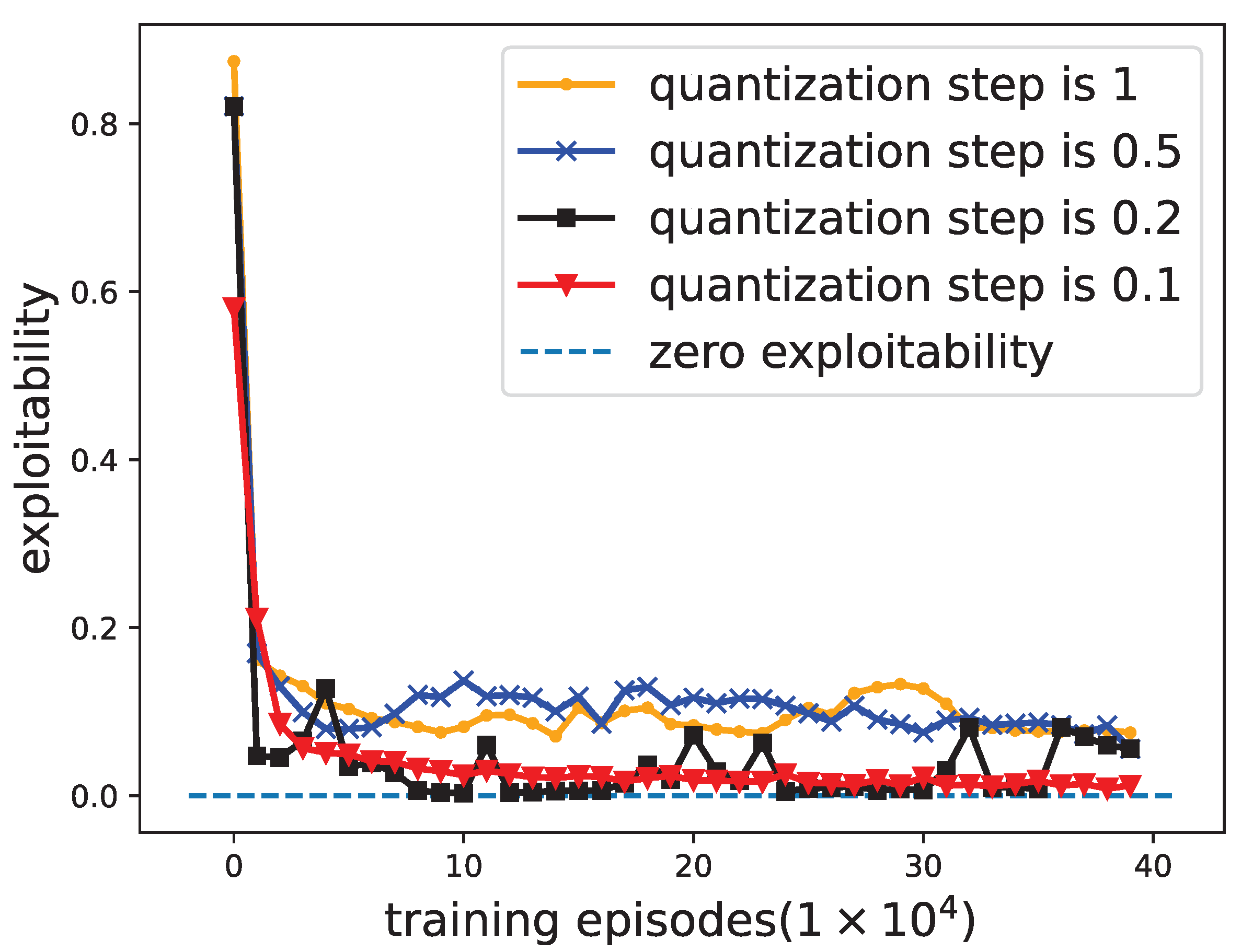
To verify whether the competition between the radar and the jammer can converge to an NE at the end of the training, the exploitability of the strategy profile needs to be evaluated. Exploitability is a metric that describes how close a strategy profile is to an NE [
42,
43,
44]. A perfect NE is a strategy profile
that satisfies the following conditions:
An approximate NE or
-NE is a strategy profile that satisfies the following conditions:
For a perfect NE, its exploitability is 0. The exploitability of
-NE is
. The closer the exploitability is to 0, the closer the strategy profile is to the NE. The exploitability curves under different quantization steps are shown in
Figure 9.
It can be seen from
Figure 9 that, under different quantization steps, the exploitability curves gradually decrease and are close to 0. The exploitability when the quantization step is 0.1 and 0.2 can converge to 0. When the quantization step is 0.5 and 1, the exploitability converges to 0.05 and 0.07, respectively. This shows that the strategy profile of the radar and jammer can achieve an approximate NE under different quantization steps.
Conclusion: If the quantization step of jamming power is smaller, the total number of jammer actions will increase accordingly. Therefore, the jammer could explore the optimal jamming strategy so that the game between the radar and the jammer can achieve a real NE.
5.3. Visualization of Approximate Nash Equilibrium Strategies
Section 5.2 shows that the game between the radar and the jammer can converge to an approximate NE under different quantization steps of jamming power. Therefore, this subsection visualizes the approximate NE strategies. Through
Figure 3 and
Figure 7, the corresponding relationship between the action number and action vector can be understood. The radar action vector is transformed into frequency, and the jammer action vector is transformed into power percentage for strategy research.
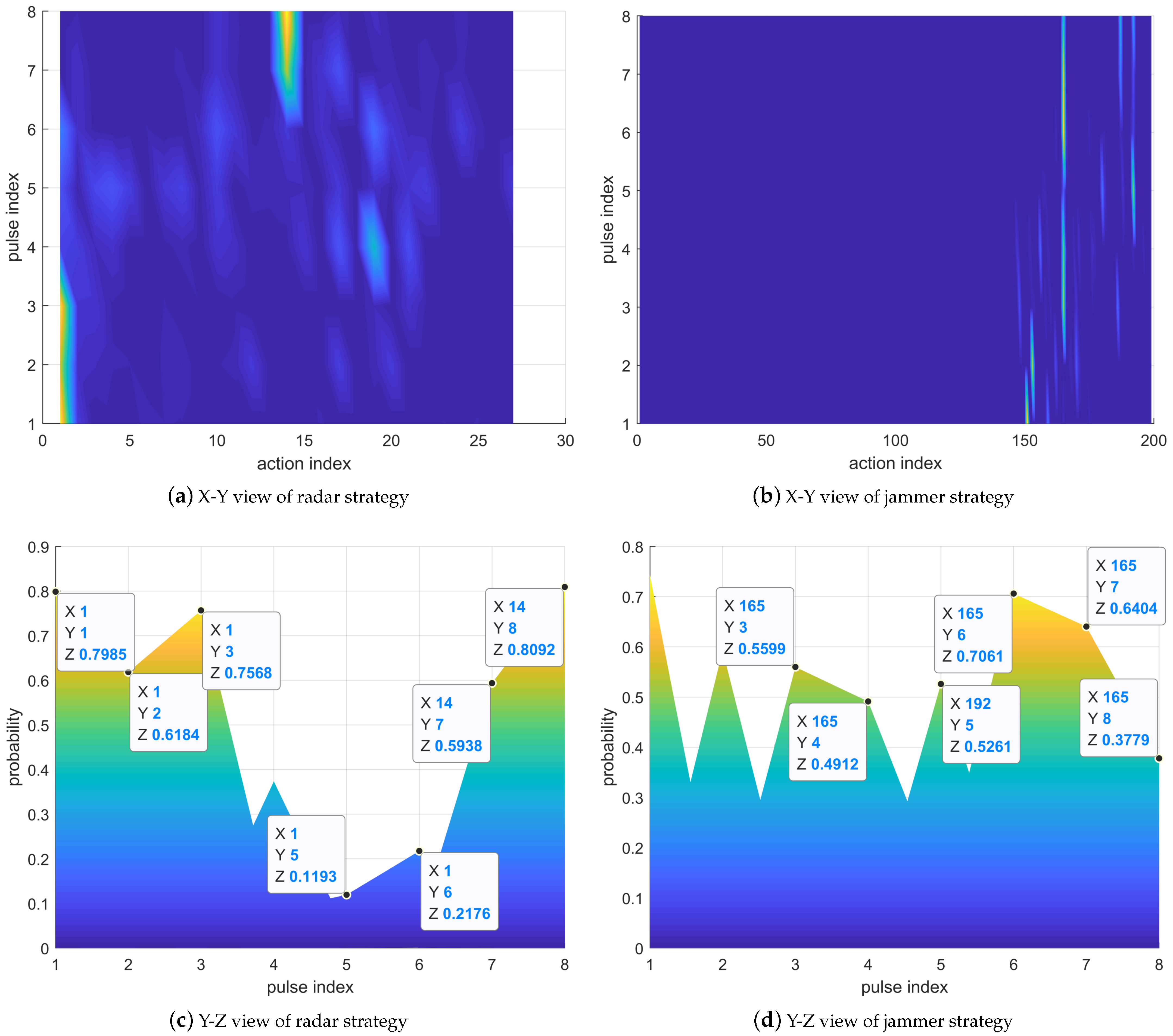
The strategies of the radar and jammer can be expressed in a three-dimensional coordinate system, in which the x-axis represents the action index, the y-axis represents the pulse index, and the z-axis represents the probability. Therefore, the meaning of the coordinates of any point is that the probability of choosing action x at the yth pulse is z.
In
Figure 10,
Figure 11,
Figure 12 and
Figure 13, (a) and (b) are the X-Y views of their strategies. The X-Y view shows the probability distribution of the radar or jammer’s selection action on each pulse. (c) and (d) are the Y-Z views of their strategies. From the Y-Z view, it can be seen that the radar or jammer selects the action with the highest probability on each pulse.
In
Figure 10, the radar prefers to select Actions 1 and 14, indicating that the carrier frequency combination of the transmitted signal is
and
, respectively. The jammer tends to choose actions 165 and 192, representing that the power ratio allocated to
,
, and
is
and
.
. The larger the RCS, the stronger the target echo power, so the jammer will allocate more power to reduce the SINR of the radar receiver. Jammer Action 192 allocates the most jamming power to
, while there is little difference in jamming power between
and
. Thus, the radar should choose
with a larger RCS, corresponding to Radar Action 14. Jammer Action 165 allocates the most jamming power to
, so the radar selects
with the largest RCS, corresponding to Radar Action 1.
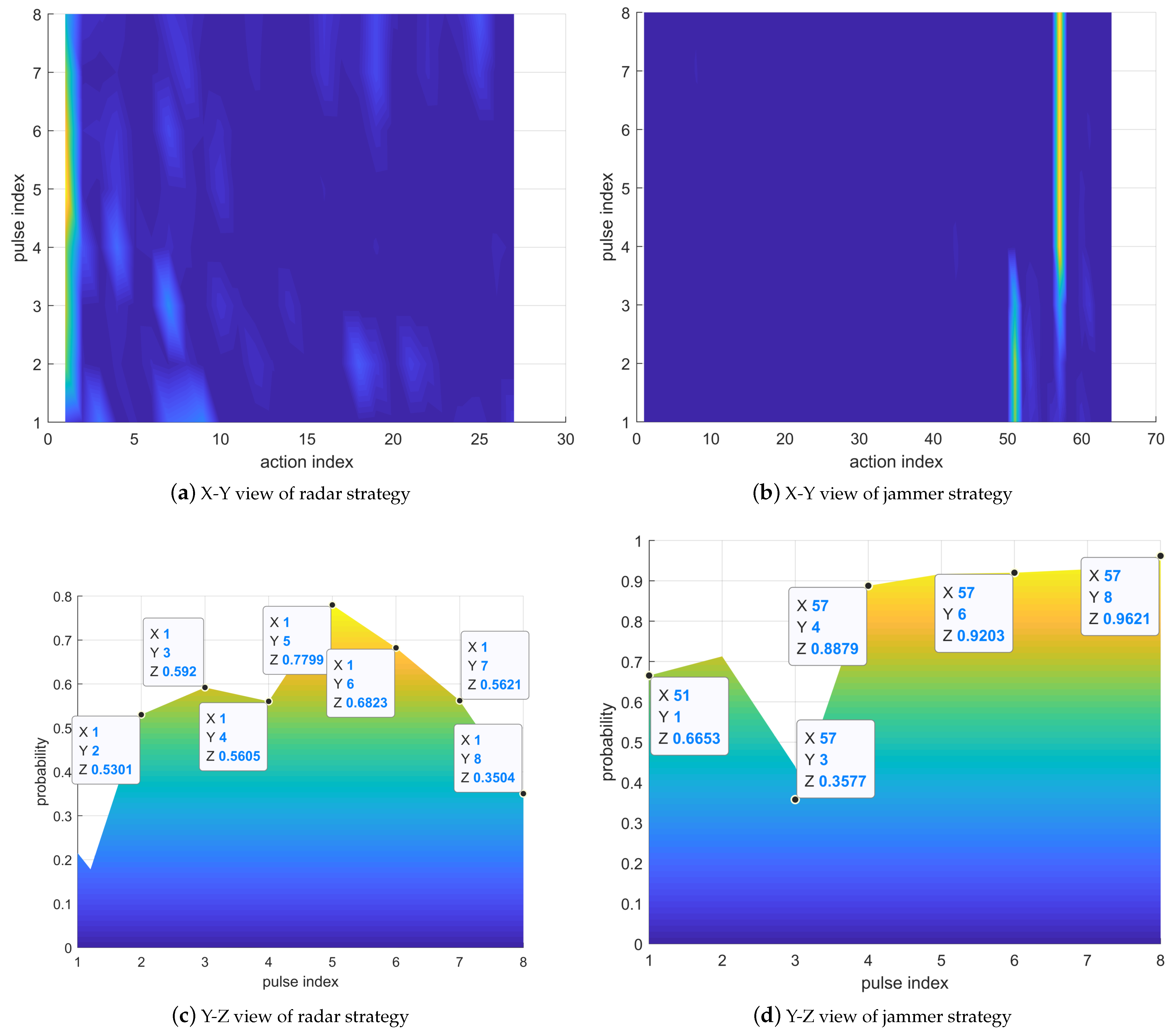
In
Figure 11, the radar selects Action 1 with the highest probability. The jammer tends to select Action 57, indicating that the power allocated to the three frequencies is
. Although the power allocated by Jammer Action 57 to
is the smallest, the RCS corresponding to
is also the smallest, and the echo power is correspondingly the smallest. The jamming power of
and
is the same, but the RCS of
is the largest. Therefore, the radar selects
, that is Action 1, which can ensure the maximum output SINR.
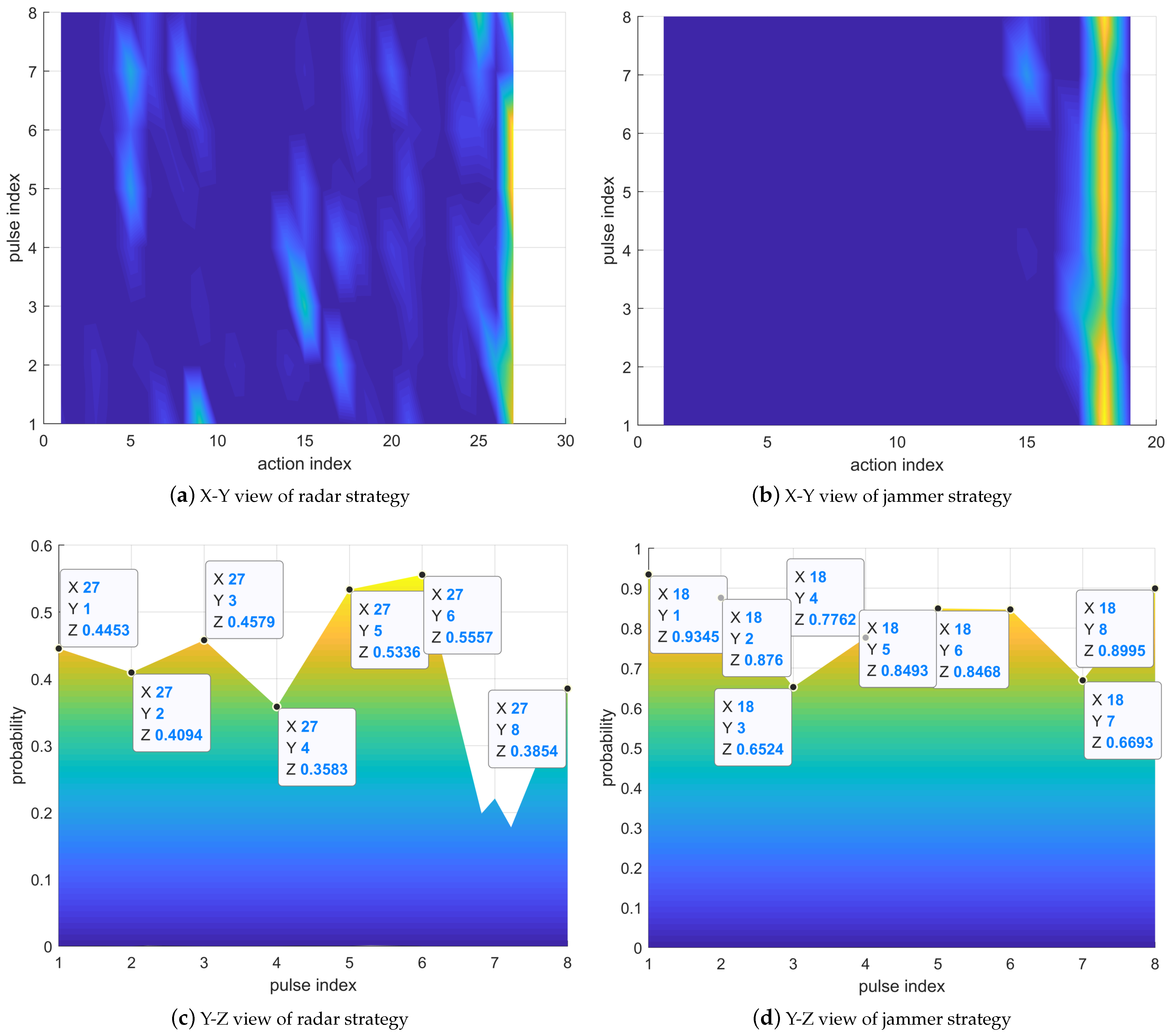
In
Figure 12, the radar selects Action 27, meaning that the combination of the carrier frequency of the transmitted signal is
. The jammer selects Action 18, representing the power allocation scheme as
. The strategy of the jammer is to evenly distribute the power to the two frequencies with the first- and second-largest RCS. At this time, the radar selection Action 27 can ensure that all subpulses will not be jammed and the radar can obtain a larger SNR.
In
Figure 13, the radar selects Action 14, which means the carrier frequency combination of the transmitted signal is
. The jammer selects Action 10, representing that the power allocation scheme is
, that is all the power is allocated to
with the largest RCS. In this case, the quantization step of power is 1, so the jammer can only use all the jamming power to jam one frequency. At this time, the subcarrier of the subpulse of the radar is all
, which is the frequency of the second-largest RCS. In this way, it can not only avoid being jammed, but also ensure a large output SNR.
In these four different scenarios, when the game converges to the NE, the strategy of the jammer is that it does not perform the look-through operation. This shows that, when the jammer is regarded as an agent, it can learn the carrier frequency information of the radar through the interaction with the radar, so it only needs to optimize the power allocation strategy. In real electronic warfare, due to the limited confrontation time, the jammer cannot fully know the available frequencies of the radar, that is the jammer needs to intercept the subpulse of the radar most of the time, which indicates that the strategy of the jammer must deviate from the NE. Therefore, the radar can achieve better performance.
It can also be seen from
Figure 10,
Figure 11,
Figure 12 and
Figure 13 that, no matter what the quantization step of jamming power is, the NE strategies of the radar and the jammer are mixed strategies. The radar and the jammer select actions from their respective action sets with a probability. This is the characteristic of imperfect information games.
Conclusion: Imperfect information games require stochastic strategies to achieve optimal performance [
36].
5.4. Comparison to Elementary Strategies
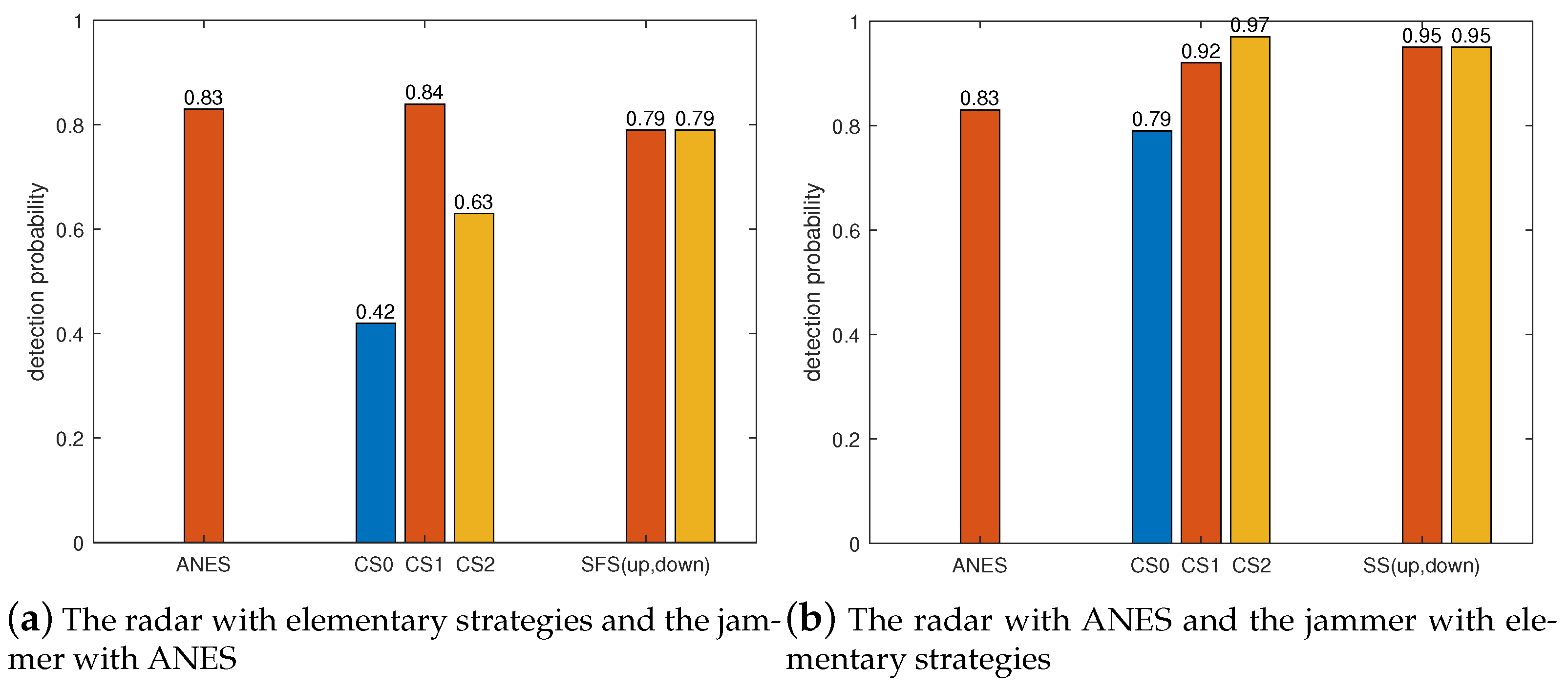
This subsection verifies the performance of the approximate NE strategies (ANESs) by comparing them with the elementary strategies.
Assume that the radar can choose two elementary strategies, which are the constant strategy (CS) and the stepped frequency strategy (SFS). The CS means that the carrier frequency of the radar is unchanged. Since the radar has three available frequencies, the CS includes three cases, denoted as CS0, CS1, and CS2. The SFS means that the carrier frequency of the radar increases or decreases step by step between pulses, and these two situations are recorded as SFS-up and SFS-down.
Two elementary strategies for the jammer were considered, which are the constant strategy (CS) and the swept strategy (SS). The CS means that the central frequency of the jamming signal remains unchanged. Similar to the CS of the radar, the CS of the jammer is also denoted as CS0, CS1, and CS2. The SS is similar to the SFS of the radar, and these two situations are recorded as SS-up and SS-down.
We made one side of the radar and jammer adopt the ANES, and the other side adopts the elementary strategies. In addition to the elementary strategies, the radar and the jammer also adopt the ANES as a comparison. The results of 1000 Monte Carlo experiments are shown in
Figure 14,
Figure 15,
Figure 16 and
Figure 17.
In
Figure 15, the detection probability of the radar adopting CS0 and the ANES is the same because these two strategies are similar in this jamming situation.
Similarly, in
Figure 16, since the CS2 and ANES of the radar are the same, there is little difference in their detection performance.
In
Figure 17, the ANES of the radar is the same as CS1, and the ANES of the jammer is the same as CS0. Therefore, the performance of one side adopting the ANES and the other taking the elementary strategy is basically the same as that of both adopting the ANES.
From
Figure 14,
Figure 15,
Figure 16 and
Figure 17, the practical implication of the NE can be known, that is, as long as one side deviates from the NE, its performance will decrease. For the jammer, performance degradation refers to an increase in the detection probability of the radar.
Conclusion: The approximate NE strategies obtained in this paper are better than the elementary strategies from the perspective of detection probability.
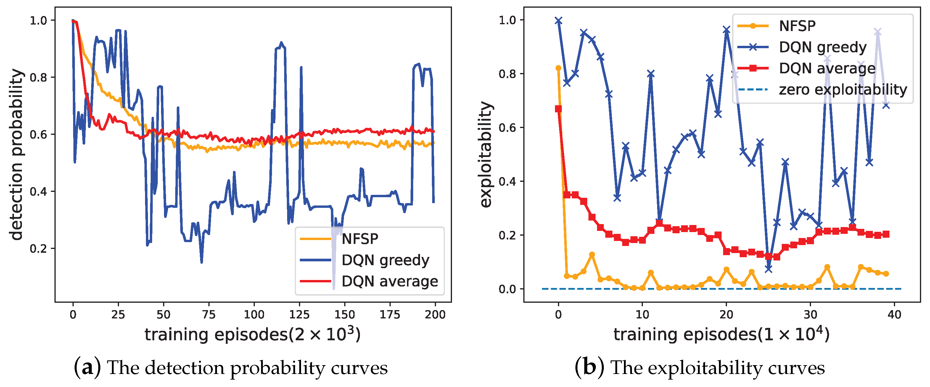
5.5. Comparison to DQN
This subsection discusses the performance of the DQN in multi-agent imperfect information games. Two forms of the DQN were considered: DQN greedy and DQN average. DQN greedy chooses the action that maximizes the Q value in each state, so it learns a deterministic policy. DQN average draws on the idea of NFSP and also trains the historical average strategy through the supervised learning model, but the average strategy does not affect the agent’s decision. Therefore, the agent chooses an action only based on at each moment, not based on a mixed policy. DQN average can be achieved by setting the anticipatory parameter in the NFSP algorithm. Because the NFSP agent in this paper solves the best response by the dueling double-DQN, DQN greedy and DQN average also adopt this method.
In
Figure 18, the detection probability and exploitability curves of DQN greedy fluctuate markedly. Its exploitability cannot converge to 0, indicating that DQN greedy cannot achieve NE. Although the training curve of the detection probability of DQN average can be stable, its policy is highly exploitable. DQN average cannot reach an NE either.
Conclusion: DQN greedy learns a deterministic policy. Such strategies are insufficient to behave optimally in multi-agent domains with imperfect information. DQN average learns the best responses to the historical experience generated by other agents, but the experiences are generated only based on
. These experiences are both highly correlated over time and highly focused on a narrow distribution of states [
36]. Thus, the DQN average performs worse than NFSP.
5.6. Performance Comparison with Existing Methods
To verify the effectiveness of the strategy obtained in this paper, a comparison between the proposed method and existing resource allocation methods was designed. The work in [
17] is the strategy design problem based on RL, so the radar and the jammer interact with one of them as the agent and the other as the environment when applying this method to the established model of this paper. The strategy for the radar and jammer is solved independently rather than based on game theory. The work in [
24] was based on the Stackelberg game and concluded that the jamming strategy is related to the target characteristic when the signal power is fixed. The method proposed in [
25] was applied to the non-resource allocation scene, and the radar echo was processed by directly eliminating the jammed pulse. In addition to the above-mentioned methods, there is a common and without loss of generality method of allocating all power to the frequency with the second-largest RCS. This allocation strategy was proven by [
25] to be feasible. This allocation method is denoted as a constant allocation strategy (CAS). The comparison result is given in
Table 7.
In
Table 7, in addition to the proposed method in this paper, the exploitability of the other existing allocation methods cannot reach 0. Therefore, only the strategy obtained in this paper is an NE.
6. Conclusions
In this paper, the intelligent game between the subpulse-level FA radar and the self-protection jammer under the jamming power dynamic allocation was investigated. Specifically, the discrete allocation model of jamming power was established and the corresponding relationship between the quantization step of power and the available actions of the jammer was obtained. Furthermore, an extensive-form game model was used to describe the multiple-round sequence decision-making characteristics between the radar and jammer. A detection probability calculation method based on SAGC was proposed to evaluate the competition results. Then, due to the feature of the imperfect information game between the radar and jammer, we utilized NFSP, an end-to-end DRL method, to solve the NE of the game. Finally, simulations verified that the game between the radar and the jammer can converge to the approximate NE under the established model, and the approximate NE strategies are better than the elementary strategies from the perspective of detection probability. The comparison of NFSP and the DQN demonstrated the advantages of NFSP in finding the NE of imperfect information games.
In the future, we should investigate the radar anti-jamming game with the continuous allocation of jamming power, in which the jammer has a continuous action space, and an algorithm to design the strategy for the radar and jammer should also be proposed.


