Article

Framework for Geometric Information Extraction and Digital Modeling from LiDAR Data of Road Scenarios

1
School of Transportation, Southeast University, #2 Southeast University Road, Nanjing 211189, China
2
China Design Group Co., Ltd., Nanjing 210014, China
3
School of Civil Engineering, Beijing Jiaotong University, No.3 Shangyuancun, Beijing 100044, China
*
Author to whom correspondence should be addressed.
Remote Sens. 2023, 15(3), 576; https://doi.org/10.3390/rs15030576
Submission received: 4 December 2022 / Revised: 8 January 2023 / Accepted: 16 January 2023 / Published: 18 January 2023

Abstract

:
Road geometric information and a digital model based on light detection and ranging (LiDAR) can perform accurate geometric inventories and three-dimensional (3D) descriptions for as-built roads and infrastructures. However, unorganized point clouds and complex road scenarios would reduce the accuracy of geometric information extraction and digital modeling. There is a standardization need for information extraction and 3D model construction that integrates point cloud processing and digital modeling. This paper develops a framework from semantic segmentation to geometric information extraction and digital modeling based on LiDAR data. A semantic segmentation network is improved for the purpose of dividing the road surface and infrastructure. The road boundary and centerline are extracted by the alpha-shape and Voronoi diagram methods based on the semantic segmentation results. The road geometric information is obtained by a coordinate transformation matrix and the least square method. Subsequently, adaptive road components are constructed using Revit software. Thereafter, the road route, road entity model, and various infrastructure components are generated by the extracted geometric information through Dynamo and Revit software. Finally, a detailed digital model of the road scenario is developed. The Toronto-3D and Semantic3D datasets are utilized for analysis through training and testing. The overall accuracy (OA) of the proposed net for the two datasets is 95.3 and 95.0%, whereas the IoU of segmented road surfaces is 95.7 and 97.9%. This indicates that the proposed net could accomplish superior performance for semantic segmentation of point clouds. The mean absolute errors between the extracted and manually measured geometric information are marginal. This demonstrates the effectiveness and accuracy of the proposed extraction methods. Thus, the proposed framework could provide a reference for accurate extraction and modeling from LiDAR data.

Graphical Abstract

1. Introduction

As-built roads have received much more attention from road administration agencies after years of operation, which requires extensive field measurements to update the corresponding information based on a data model or technology, such as Building Information Modeling (BIM) [1]. Geometric and semantic information on as-built roads and infrastructures is essential to cover a wide range of topics, including asset management and road safety inspection [2,3]. Advanced information and sensing technologies have been increasingly applied in road maintenance and management with the increase in the number of as-built roads and higher requirements of construction management [4]. Light detection and ranging (LiDAR) is a reliable and efficient technology widely used in road geometry measurements, obstacle detection, and landscape modeling [5,6]. This technology could provide high quality point clouds [7]. However, these point cloud data do not contain semantic and geomatic information. Moreover, road scenarios are complex and contain multiple types of objects. This decreases the precision of semantic segmentation and geometric information extraction. In particular, the data gathered through LiDAR technology is a collection of unorganized, irregularly sampled, and unstructured point clouds [8], which increases the difficulty of converting the point clouds into semantic-rich models of as-built roads and different categories of infrastructures. Thus, it is important to establish an accurate and effective framework that takes, as input, point clouds from LiDAR systems and outputs a digital model to interlink 3D point clouds regarding the geometric and semantic information of as-built roads and surrounding infrastructures.
Within this context, the road surface is an important road design structure, representing the geometric information of the road. Roadside infrastructure is essential for traffic-related applications and safe operation. Hence, segmentation of road surfaces and infrastructures is the first step for generating detailed geometric elements. The studies related to road surface segmentation from point clouds have focused on three categories: structure-driven, feature–driven, and model-driven methods [9,10,11]. Structure-driven methods rely on the detection of curbs to define the road boundary and the subsequent extraction of the road surface [12]. These methods have been developed for curb detection using different data sources, including the scan lines, density and elevation of 3D point clouds [13,14], and two-dimensional geo-referenced feature (2D GRF) images generated by the projection of the 3D point clouds [15,16]. Although good results were attained from these works, the segmentation of the road surface is not robust when it is not delimited by curbs, which is the case for most non-urban roads. Feature–driven methods are performed based on previous knowledge of geometric and contextual features, such as roughness and the height of road surfaces [17,18]. However, these approaches require a substantial number of fixed thresholds, which need to be defined or tested by the user. Model-driven methods primarily refer to the semantic segmentation of road surfaces by deep neural networks. These can be largely divided into three categories [19]: projection-based [20], discretization-based [21,22,23], and point-based methods [24]. The first two methods convert the point clouds into other regular representations, such as 2D images and 3D grids. This causes information loss and incurs computation expense for the projection back to the original dimension [25]. Unlike the above methods, point-based methods (e.g., PointNet and PointNet++) directly work on the point clouds. For large-scale point clouds containing hundreds of objects, the widely employed farthest point sampling cannot efficiently and rapidly process a large number of points. Thus, the pioneering RandLA-Net [26] was proposed as a potential approach developed on the principles of random sampling (RS). However, it fails to capture wider context information for different and similar features owing to the removal of key features caused by the RS method [27].
In addition, numerous studies have examined the geometric information extraction methods based on point clouds and other data sources, such as the Geographic Information Systems (GIS) database [28,29], optical images [30], or vehicle trajectory obtained by Global Positioning System (GPS) [31] or Inertial Measurement Units (IMU) [32]. According to the above analysis, the accuracy of geometric element extraction is severely affected by the captured data sources. However, the accurate extraction of geometric information using optical images is challenging because of low illumination and inclement weather. Furthermore, certain extraction methods based on trajectory data may not satisfy the requirements of a stationary system. In addition, the integrity and accuracy of the obtained trajectory are limited in complex road scenarios owing to the movement of vehicles with larger fluctuations and away from the centerline of the road.
Finally, and in the context of digital modeling using 3D point clouds, Justo et al. proposed a semi-automatic modeling approach for traffic signs, guardrails, and other road elements via BIM [33]. In addition, they modeled the alignment and centerline of each road lane on a highway through BIM and GIS [34]. Tang et al. developed a framework for integrating road design and pavement analysis relying on the capabilities of Dynamo [35]. However, these approaches only focused on separate objects, rather than considering the integration of the road and other infrastructures in a real-world space or their relationship.
The objective of this paper is to present a framework that accepts raw point clouds from various LiDAR systems as input, and outputs an integrated digital model that represents the geometric and semantic information of the road and other infrastructure. The main contributions of this study are as follows:
(1)
An improved semantic segmentation network that accurately and efficiently divides the road surface and other infrastructure.
(2)
A series of geometric information extraction methods that can be used to obtain the road boundary and centerline, and to calculate the geometric elements of roads. These can be applied to the segmented point clouds that contain 3D coordinates and RGB information. Note that the extraction methods do not aim to be the contribution. However, these are essential for the entire workflow and would be validated if the mean absolute errors between the extracted and manually measured geometric information were marginal.
(3)
A digital modeling process that constructs a road entity model and various infrastructure components to realize a geometric representation.

2. Materials and Methods

This section is divided into four subsections. The first analyzes the point clouds obtained by different LiDAR systems. After a brief overview of the methods, a detailed description of the main processing steps is provided. In particular, point cloud semantic segmentation and the extraction of road geometric information are described. The digital modeling of road scenarios is described in detail.

2.1. Point Clouds Obtained by Different LiDAR Systems

Considering the platform type employed to install the system, there are three types of arrangements of laser scanner systems: terrestrial laser scanner (TLS), aerial laser scanner (ALS), and mobile laser scanner (MLS) [36]. A TLS is a stationary system consisting of a LiDAR device mounted on a tripod or other type of stand. It is capable of obtaining high-resolution scans of complex scenarios. The point clouds captured by TLS contain 3D coordinates, RGB information, and intensity [37]. With regard to ALS, the laser scanner is installed on an aircraft (typically an airplane) based on GNSS receivers and IMU. The ALS can record the 3D coordinates and intensity of each echo, and colorize point clouds through digital photographs captured by a calibrated camera [38]. Finally, the MLS is integrated with multiple on-board sensors comprising a GNSS system, an IMU, and a DMI. However, in certain cases, the data processing methods used in TLS or ALS cannot be directly applied to MLS. This is owing to differences in the manner of data acquisition, mainly the geometry of the scanning and point density [39]. Therefore, our study is implemented based on per-point features (e.g., 3D coordinates and RGB information). It focuses on the content of acquired data rather than the LiDAR systems, thereby ensuring the universality of the proposed methods.

2.2. Methods Overview

The methodology proposed in this paper is divided into three steps (see Figure 1): (1) semantic segmentation, (2) geometric information extraction, and (3) BIM technology for digital modeling. The raw point cloud data do not possess semantic and geomatic information, and road scenarios are complex and contain multiple types of objects. Therefore, we first segment the road surfaces and infrastructures in the process of semantic segmentation. More specifically, the improved semantic segmentation network is proposed in Step 1. Based on a fundamental foundation of SCF-Net, the aggregated attention pooling module is improved to describe the difference and similarity of local features. Then, 3D coordinates and radial distributions are gathered to enrich global contextual features and preserve the complex geometric structure of point clouds. The road surfaces and other categories of infrastructure are segmented by this procedure. In Step 2, the road boundary and centerline are extracted by the alpha-shape method and Voronoi diagram (or Thiessen-Polygons) method based on the segmented road surfaces. Subsequently, the geometric information is obtained from the 3D coordinates of the road boundary and centerline. Finally, the road centerline and geometric information is imported to generate a road route through Dynamo. Adaptive road components are developed and placed to form a complete road entity model based on the generated road route. Given the segmented infrastructures in Step 1, the locations of infrastructures are determined and fitted. The road entity model and various infrastructure components, such as guardrails and buildings, are constructed and arranged using Revit software. Thereby, the details of vegetation and other elements are manually adjusted based on the imported point clouds, and the digital road scenario is established.

2.3. Semantic Segmentation of Point Clouds

The large scale of point clouds incurs high computational and memory costs owing to the wide space of road scenarios, including the road surface, vegetation, infrastructure, buildings, and other categories of objects. Consequently, an efficient and lightweight deep neural network needs to be applied to directly infer per-point semantics for large-scale point clouds, and thereby realize multi-object recognition and segmentation. Large-scale point cloud semantic segmentation networks have been proposed, such as RandLA-Net and SCF-Net. SCF-Net can achieve high efficiency using the RS method and generate point-wise representations of spatial information. However, the RS method would unintentionally discard key features [40]. It is worth mentioning that the collected point clouds may include noise and unclear objects at a distance from the sensor. These affect the accuracy of semantic segmentation. It is difficult to reflect the different and similar features of local point clouds because the point clouds would be inadequate and sparse during the sampling process. To address these subproblems, we propose an improved SCF-Net for raw point clouds to aggregate the different and similar local contextual features, and optimize global contextual features. This would enhance the capability to learn effective spatial contextual features from large-scale point clouds. We introduce the proposed module in detail in this section and describe the architecture of the improved SCF-Net in the following subsection.

2.3.1. Improved SCF Module

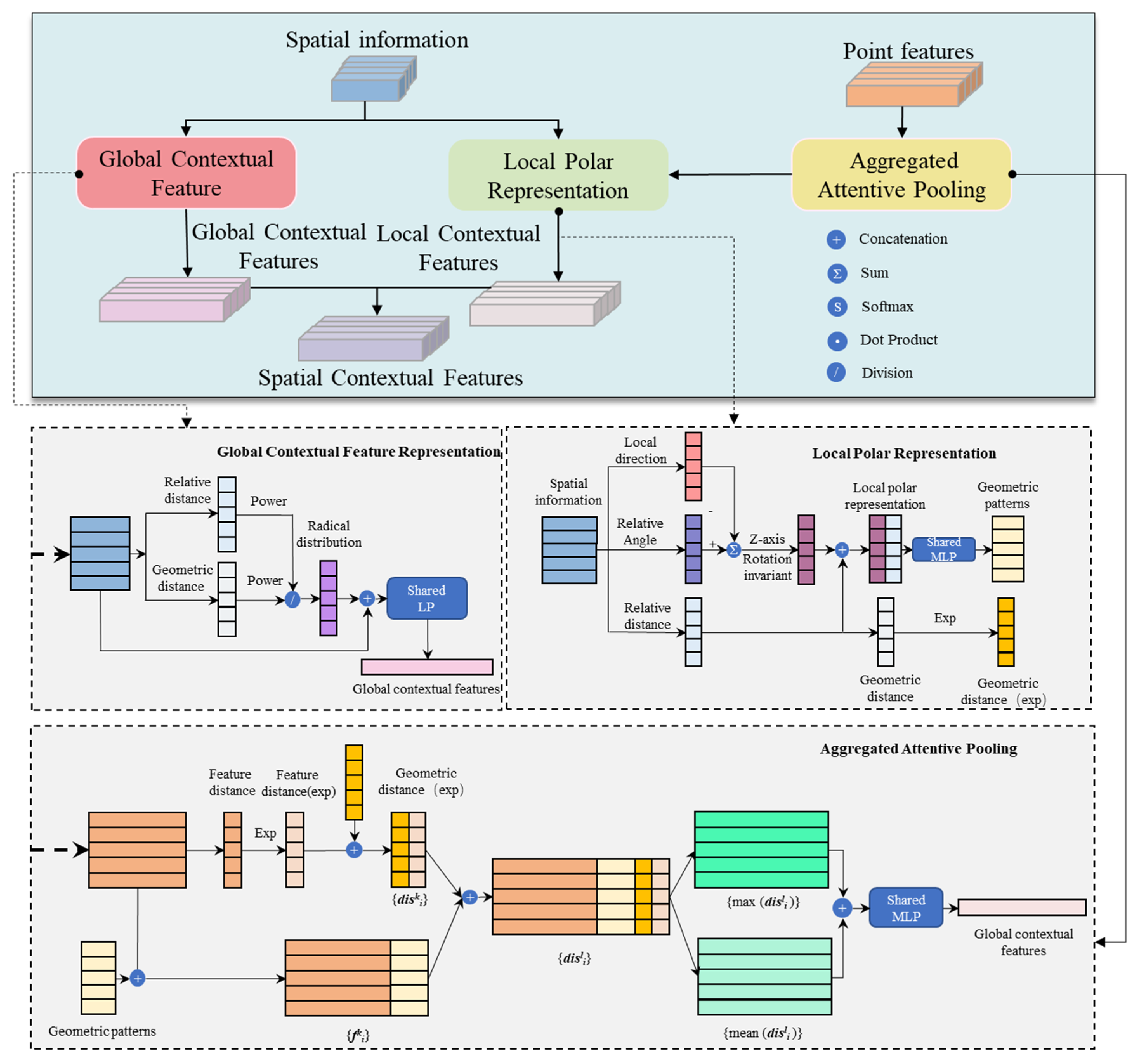
We improved the SCF module to extract local and global contextual features of point clouds. It consists of three blocks: local polar representation (LPR), aggregated attentive pooling (AAP), and global contextual feature representation (GCFR). We introduce the architecture of the improved SCF-Net. It has an encoder-decoder with the SCF module.
It is observed that the improved SCF module is applied to aggregate the local maximum and mean features of neighboring points to extract more local contextual features and reduce the redundant information in an AAP neural unit. In a GCFR neural unit, 3D coordinates and radial distributions are utilized as global contextual features to represent the distribution of point clouds in 3D space (see Figure 2).
  • Local Polar Representation
It is notable that, in certain real scenarios, segmentation performance is hindered by different orientations of the same category of objects. For example, vehicles parked in different orientations on the roadside may be misconstrued as roadside infrastructures [41]. We apply the method proposed by Fan [27] to reduce the influence of object orientation on the geometric features. Evidently, the LPR unit is established in the polar coordinate system that is invariant along the z-axis. Furthermore, the local context of point clouds is converted from Cartesian coordinates to polar coordinates.
First, a point and its k-nearest neighboring points are obtained in the polar coordinate system. Thereafter, the geometric distance and original relative angles are calculated. Then, the center-of-mass of the neighboring points is determined, and the local direction is defined from a point to its center-of-mass. In addition, the updated relative angles are obtained by the original relative angles and relative angles. Finally, the updated relative angles and geometric distance are combined as the geometric patterns.
2.
Aggregated Attentive Pooling
The AAP unit is developed by integrating the local and neighboring point features to measure geometric details among large-scale point clouds and learn local contextual features. In an AAP unit, the geometric distance, point features, and geometric patterns are obtained as inputs. This proposed unit entails the following steps:
Computing the feature distance: The L1 norm and mean function are used to calculate the feature distance between the input feature vectors of the i-th point and its k-th neighboring point [27]. This can be expressed as
d i s i f k = mean ( | v ( i ) | | v ( k ) | )
where d i s i f k denotes the feature distance, | | is the L1 norm, and mean (·) is the mean function. v(i) and v(k) denote feature vectors of the i-th point and its k-th neighboring point, respectively.
Determining the attentive pooling weights: The geometric distance and feature distance can measure the correlation among points in the world and feature space. The smaller the distance, the higher their relevance. Meanwhile, the weights lie in [0,1]. Hence, the geometric distance and feature distance are transformed through a negative exponential, and combined to define the aggregated distance d i s i k :
d i s i k = concat ( exp ( d i s i g k ) , exp ( d i s i f k ) )
where d i s i g k and d i s i f k are the geometric distance and feature distance, respectively.
Given the aggregated distance d i s i k , we combine point features f ι κ to obtain the set of local features d i s i l through a concatenation operator. Then, we use a shared MLP followed by Softmax to learn the attentive pooling weight w i k for d i s i l .
Calculating local contextual features: First, the maximum features max k ( d i s i l ) from the neighboring point features are directly collected to show the local distinctness. Then, the neighboring point mean features mean k , w k i ( d i s i l ) are defined by re-weighting the neighboring point features with w i k to closely gather similar local context. Finally, we combine the two types of features to precisely capture and learn local contextual features f i L by utilizing the neighboring point features.
f i L = concat ( max k ( d i s i l ) , mean k , w i k ( d i s i l ) )
3.
Global Contextual Feature Representation
Given the local contextual features, the context among the neighboring points is not sufficiently discriminative for semantic segmentation. The global contextual features can be used to learn complex geometric structures and enrich the global context from 3D points. These two contextual features can be concatenated to obtain spatial contextual features.
It is noted that different objects of the same category may have certain differences in global spatial features owing to different locations and scenarios. Furthermore, their geometric architectures are generally similar. The radial distribution is utilized as the supplement of global contextual features. It reflects the distribution of point clouds in the world space [42], which is defined as follows:
r i = ρ l i ρ g i = N k i N g i ( R l i R g i ) 3
where ri is the radial distribution; ρ l i and ρ g i are the densities of the neighboring points and global point clouds, respectively; N k i and N g i are the numbers of neighboring points and global points, respectively. R l i and R g i are the local and global radii, respectively.
The radial distribution could combine the local and global information distribution and is irrelevant to the per-point distribution. Evidently, the radial distribution is insensitive to marginal geometric deformations, thereby reserving the global information and geometric structures. In addition, the 3D coordinates of a point p i are used to represent the location of local neighboring points. Therefore, 3D coordinates are combined with radial distribution as global contextual features. This is defined as follows:
f i g = concat ( MLP ( x i , y i , z i ) , r i )

2.3.2. Architecture of Improved SCF-Net

In this subsection, the improved SCF module is embedded in a standard encoder-decoder architecture to yield the improved SCF-Net. It consists of fully connected layers, and encoder and decoder layers (see Figure 3). A fully connected layer is first used to extract the per-point features. In addition, five encoders are used to reduce the point cloud size and increase the feature dimension. More specially, the number of point clouds is downsampled through the RS method. The improved module can learn effective spatial contextual features to prevent loss of valid information caused by the RS method. Then, decoder layers are used after the above encoder layers. The encoded feature dimension is then upsampled through a nearest-neighbor interpolation. The upsampled features are concatenated with the intermediate features produced by the encoder layers through skip connections. Thereafter, a shared MLP is used to concatenate the features before and after sampling. Finally, three fully connected layers and a dropout layer are applied to predict the semantic labels. Furthermore, the cross-entropy loss is used for training.

2.4. Process of Road Geometric Information Extraction

The geometric information, including the horizontal alignment, vertical alignment, and cross-section of the road (particularly the elevation of intersections), needs to be obtained for the as-built survey or traffic safety analysis. Evidently, the digital elevation model (DEM) of the intersection is established to provide the basis for calculating the sight distance, analyzing traffic conflicts, and reconstructing intersections. Therefore, we propose a series of geometric information extraction methods for segmented point clouds from various LiDAR systems. To guarantee the reliability and versatility of the methods, we use 3D coordinates and RGB information as per-point features, lacking timestamps and echo times. Accordingly, certain methods based on scan lines are unsuitable for geometric information and track extraction [43,44].
Given the segmented road surface, the alpha-shape method is first used to preserve polygonal details of the finite points for boundary reconstruction [45]. The parameter α identifies the radius of the rolling circles around the road, which controls the precision of the boundary [46]. Thereafter, the centerline can be extracted by the Voronoi diagram (or Thiessen-Polygons) method depending on the calculated road boundary points. Moreover, extraneous lines are removed by several iterations and a minimum threshold [47,48]. Finally, the geometric information calculations based on the road boundary and centerline entail the following steps:
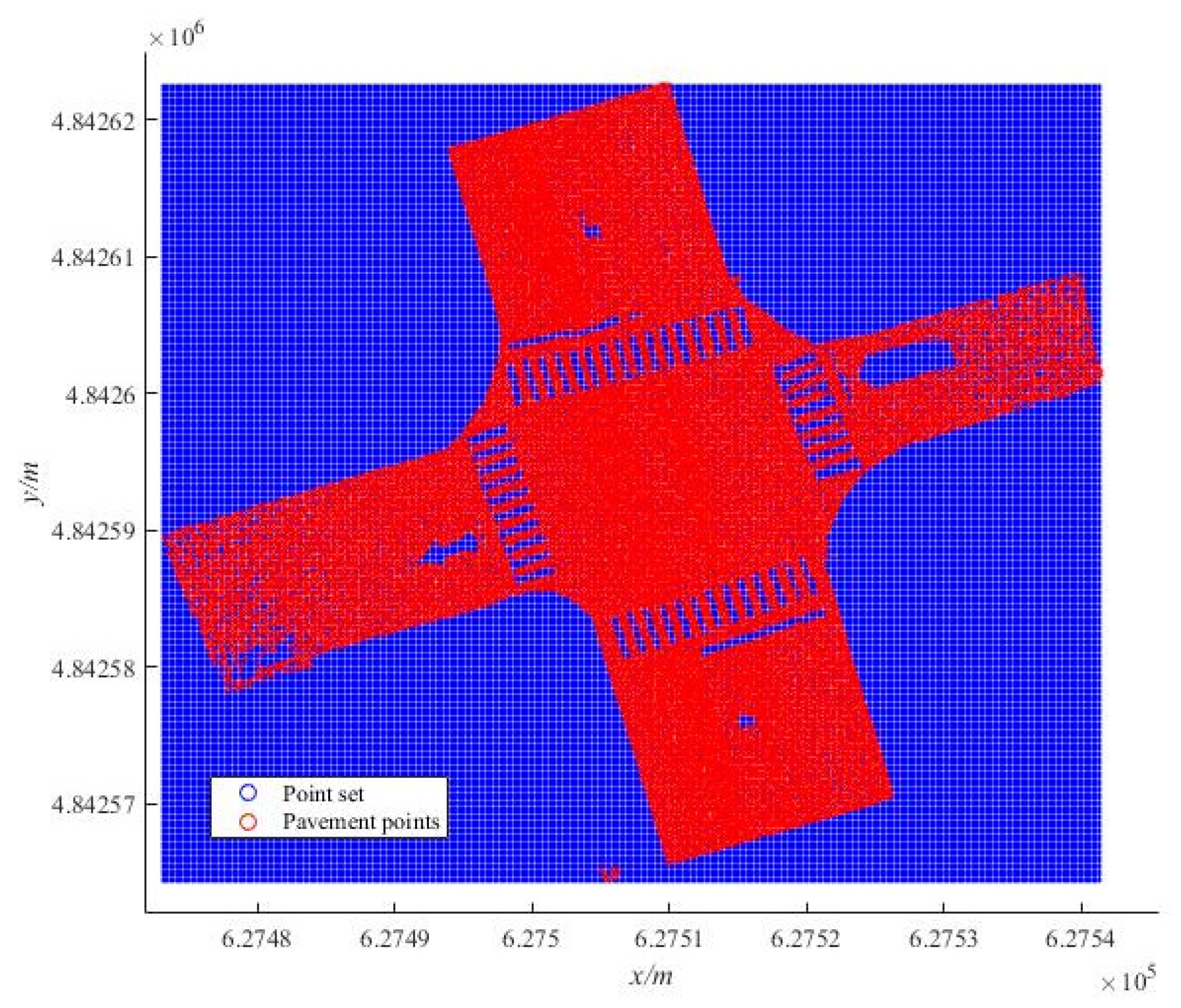
DEM of the intersection: Owing to the different densities of the captured road surface points, a uniformly distributed point set is first generated to calculate the elevation of the intersection. In particular, the range of the uniformly distributed point set is generated from xmin to xmax and from ymin to ymax. This forms a series of points with ε intervals. Thus, the number of the point set is y max y min ε × x max x min ε (‘   ’ implies floor function). Moreover, the inShape function in MATLAB is used to assess and reserve the road surface points within the extracted boundary of the intersection. The elevation of each point in the point set is determined by the interpolation method based on the elevation and distance of two adjacent road surface points. This can be expressed as
Z i = d i b d i a + d i b · z i a + d i a d i a + d i b · z i b
where Z i denotes the elevation of the i-th point in the point set; z i a , z i b are the elevations of the two adjacent road surface points nearest to the i-th point; and d i a , d i b are the distances between the two adjacent road surface points and the i-th point.
Thus, the DEM of the intersection is established by integrating the elevation of the point set and the existing road surface points. Similarly, the DEM of the road can be constructed on the surface points within the road boundary.
Horizontal information: To decrease the difficulty of geometric information calculations, the curved road is transformed into a straight line by applying the coordinate transformation matrix of Equation (7). The original surface points are converted into transformed points based on the coordinates of the road centerline. Thus, the vertical and forward directions of the road are determined as the OX and OY directions, respectively. The horizontal alignment is generated by the transformed centerline.
[ X Y Z ] = [ cos ( θ ) sin ( θ ) 0 sin ( θ ) cos ( θ ) 0 0 0 1 ] ( [ x y z ] [ x 0 y 0 z o ] ) + [ x 0 y 0 z o ] , θ = ( π 2 ϕ )
where X , Y , Z denote the 3D coordinates of the transformed point; θ is the transformation angle; ϕ is the grade of the road centerline; x, y, z are the 3D coordinates of the original surface points; and x0, y0, z0 are the origin coordinates of the road centerline.
Vertical information: The elevation of the centerline is utilized to calculate the longitudinal slope of the road. Moreover, the relative elevation difference and horizontal distance of the centerline are obtained. The quotient of the two values is computed as the longitudinal slope, which can be express as:
i j = H j + 1 H j W j + 1 , j = H j + 1 H j ( X j + 1 X j ) 2 + ( Y j + 1 Y j ) 2
where Hj, Hj+1; Xj, Xj+1; and Yj, Yj+1 denote the elevations, X-coordinates, and Y-coordinates, respectively, of the j-th and j + 1-th points of the centerline.
Cross-section information: First, the cross-sectional profile is represented in a vertical plane. It is computed as being perpendicular to the plane defined by the forward directions of the road. Thereafter, the identified cross-sectional profile is divided into left and right sides based on the centerline. The road width is calculated as the difference between the left and right sides. The least square method is then used to fit the cross-sectional profile on both sides, reducing the errors caused by the different densities of road surface points. Meanwhile, the errors between the fitting curves and the points of the profile are calculated. The slope of the fitting equation when the error is minimum is the cross slope.

2.5. BIM Technology for Digital Modeling

Based on the semantic segmentation of point clouds and the extraction of road geometric information, this study combines road 3D point clouds with BIM technology. In particular, the road entity and infrastructure modeling is established based on Dynamo and Revit. Dynamo is a visual programming software for geometric shapes, Revit diagram elements, and data interaction. The process of completing the parametric design of the road scenario entails the following steps.
To ensure that the work is feasible and effective in Dynamo, many nodes such as Code Block, NurbsCurve.ByPoints, and Data.ImportExcel are connected for editing. The process of digital modeling entails the following steps:
Setting the coordinate system: The point cloud of the road scenario is imported in Autodesk Recap and converted into rcp format. It can be inserted in Revit software to complement information for modeling. The point cloud and Revit file are set in the same coordinate system to ensure consistency with the position and orientation.
Generation of road route: Given the extracted road centerline and geometric information, the Excel database relevant to the 3D information of each stack is established. Thereafter, Data.ImportExcel is used to import the coordinate and geometric information (stack number, horizontal and vertical coordinates, elevation) from the Excel database. Finally, the imported coordinate data is fitted to generate the road route using NurbsCurve.ByPoints.
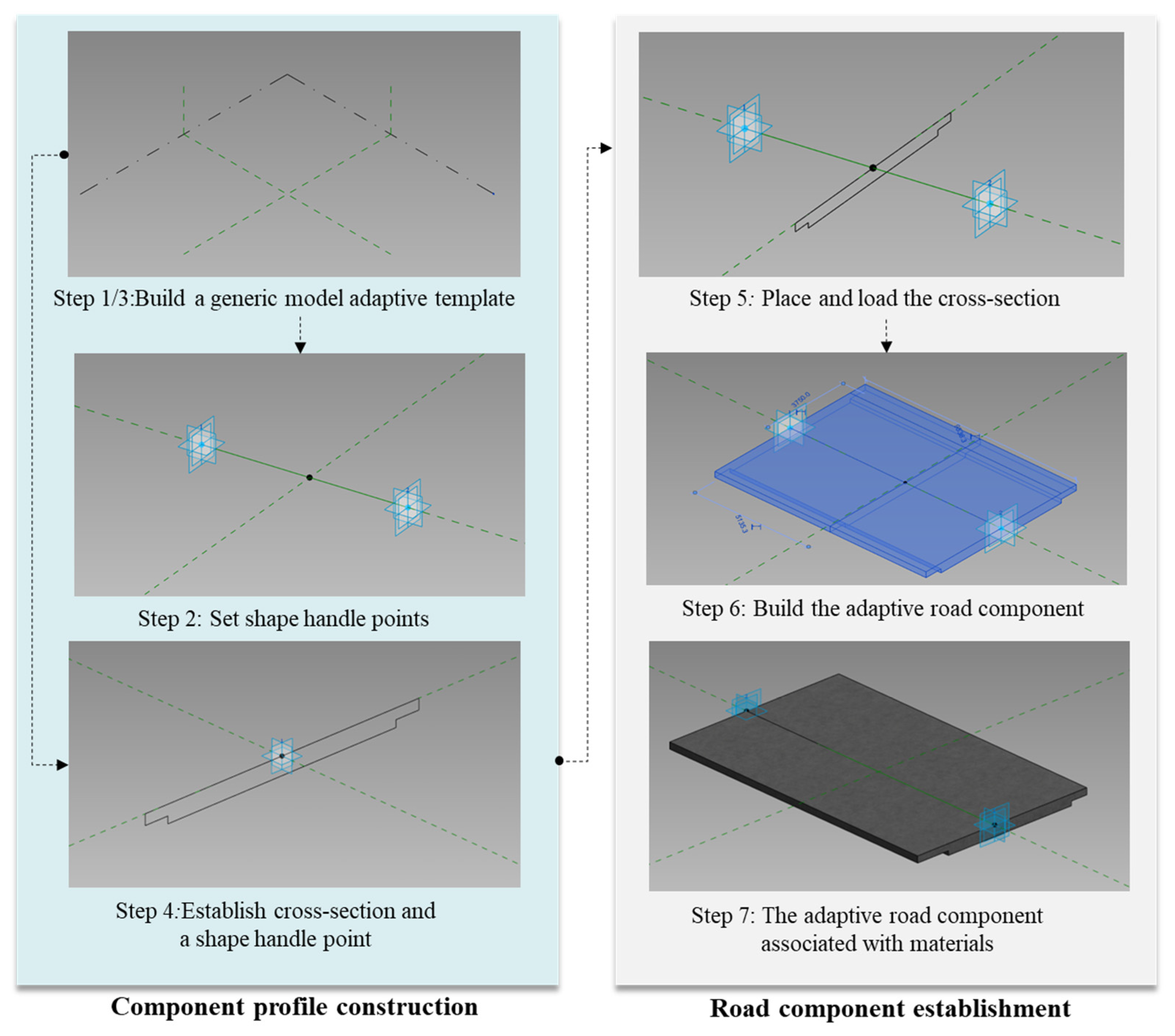
Setting adaptive road components: Considering the flexibility of an adaptive component in generative applications, we construct adaptive road components to adapt the actual road alignment. This process of generating an adaptive road component used by Revit software entails the following steps (see Figure 4).
First, a new generic model adaptive template is developed. Thereafter, the shape handle points are set and adjusted at the origin, midpoint, and destination of the adaptive component based on the direction of the road route, to ensure consistency with the design.
Additionally, another generic model adaptive template is created. In the template file, a cross-section is established. Thereby, a new shape handle point is generated and adjusted at the origin of the cross-section.
Finally, the origin of the cross-section is placed and loaded at the midpoint of the road route, generating the adaptive road component. The established adaptive road components associated with materials can be offered in the road entity model through Dynamo.
Establishment of the road entity model: First, a series of discrete coordinate data are obtained from the generated road route by equidistant interpolation. In addition, the deviation from each interpolation point to the road route is calculated in the XOY plane. The interpolation point is removed depending on the threshold value. Specifically, the processed interpolation points are allocated relying on the road alignment. When the road alignment is straight, two interpolation points are grouped as the origin and destination at the centerline of the adaptive road component. When the road alignment is a circular curve, three interpolation points are grouped as the origin, midpoint, and destination at the centerline of the adaptive road component. The cross-section is then adjusted to satisfy the requirements of widening and superelevation. For the transition curve, apart from setting the three interpolation points, additional shape handle points should be arranged at the origin, midpoint, and destination of the inner and outer roads. Accordingly, the designed adaptive components are placed among the group of interpolation points to form a complete road entity model using Dynamo.
Constructing the infrastructure components: Different categories of infrastructure components are constructed based on the semantic segmentation results. The data of the infrastructure boundary are imported through Data.ImportExcel first. The data is thereafter fitted to form boundary curves by NurbsCurve.ByPoints. Subsequently, the locations of placements are determined on the fitted boundary curves to construct different infrastructure. Finally, the infrastructure components are manually placed and constructed through Revit software.
Construction of 3D road scenario: Detailed designs are carried out for the road entity model and infrastructure components through Dynamo and Revit software. Evidently, the details of the surrounding environment are manually adjusted based on the imported point clouds. In addition, the road infrastructure assets and model information exchange and sharing can be completed based on BIM technology by adding the records regarding name, age, and maintenance.

3. Results

3.1. Datasets and Implementation Detail

In this section, we train and evaluate the improved SCF-Net on two typical large-scale point cloud benchmarks: Toronto-3D [49] and Semantic3D [50]. The following includes a description of the datasets and the detailed implementation. Toronto-3D is a dataset related to urban roadways captured by the MLS system. It consists of four sections. Each point cloud owns the attributes of 3D coordinates, RGB information, intensity, GPS time, and scan angle rank. Semantic3D is related to urban and rural scenarios including streets, intersections, and rural roads. The TLS system is used for recording these scenarios. The raw 3D points are represented by 3D coordinates, RGB information, and intensity in the experiments.
Owing to the different acquired platform type, the attributes of each captured point cloud are dissimilar. Meanwhile, the manner of data acquisition affects the geometry of the scanning and point density. Therefore, our study uses two datasets from different LiDAR systems and focuses on the common attributes of acquired data to ensure the application of the proposed net. Because the intensity is significantly affected by the environment and illumination, we use 3D coordinates and RGB information of points for training and testing.
The experiments are implemented in Tensorflow on a server with NVDIA GTX-1080 TI GPU and CUDA 11.5. We use the Adam optimizer with default parameters. For example, the initial learning rate and batch size are set as 0.01 and 5, respectively. The network is trained for 100 epochs with a dropout ratio of 0.5. The number of neighbors is set to 16 (k = 16).

3.2. Semantic Segmentation on Benchmarks

We compare the proposed net with other state-of-the-art methods. We use the mean IoU (mIoU) and overall accuracy (OA) as standard metrics to evaluate the semantic segmentation of the proposed net on the Toronto-3D and Semantic3D datasets.

3.2.1. Evaluation on Toronto-3D

We select L002 as a test set for its smaller size and balanced number of points of each label. The mIoU and OA of the total eight categories are compared in Table 1. The visual comparison between point clouds and semantic segmentations is shown in Figure 5.
As Table 1 indicates, our method outperforms the other methods in three of the eight categories; i.e., road surface, road marking, and fence. In particular, the IoU of the road surface in dense scans is higher than 95%. The proposed net is marginally inferior to RandLA-Net in terms of mIoU, but better in terms of OA. This is mainly owing to the suboptimal segmentation in the category of vertical objects (such as buildings, utility lines, and poles), which marginally reduces the mIoU. Figure 5 presents certain qualitative results at the intersection of L002. However, road markings could not be identified. These can be accurately extracted by the additional intensity and other information.

3.2.2. Evaluation on Semantic3D

In this work, we submit the results to the server and infer the dense scenes of the semantic-8 test set. The quantitative results are reported in Table 2. We consider an irregular road as an example because the ground truth of the test set is not publicly available. Its RGB colored point clouds and predicted segmentation results are presented in Figure 6, which shows the visualization results.
As shown in this table, our method has the best mIoU and OA among all of the methods. Furthermore, the segmentation of the road surface exhibits better performance (an IoU of 97.9%) than the other categories. The categories of natural terrain, building, cars, and trucks have an IoU of over 89%. Figure 6 indicates that the low vegetation category, with low height and discrete distribution, is straightforwardly classified as infrastructure. Most errors are caused by the low vegetation, infrastructure, and scanning artifact categories with few points and indistinct geometric structures, which renders the aggregated attentive pooling unit incapable of effectively obtaining the difference and similarity of its local features.
Meanwhile, we compared the improved SCF-Net with the SCF-Net based on the benchmark to validate the effectiveness of the improved SCF module. The results show that the proposed module could enrich the feature expression of input points’ spatial information. Thereby, it achieves a higher application value for semantic segmentation. Overall, the improved net could be applied in the semantic segmentation of large-scale point clouds, particularly for road surfaces. This could ensure the accuracy and efficiency of road geometric information extraction in the subsequent steps.

3.3. Results of Road Geometric Information Extraction

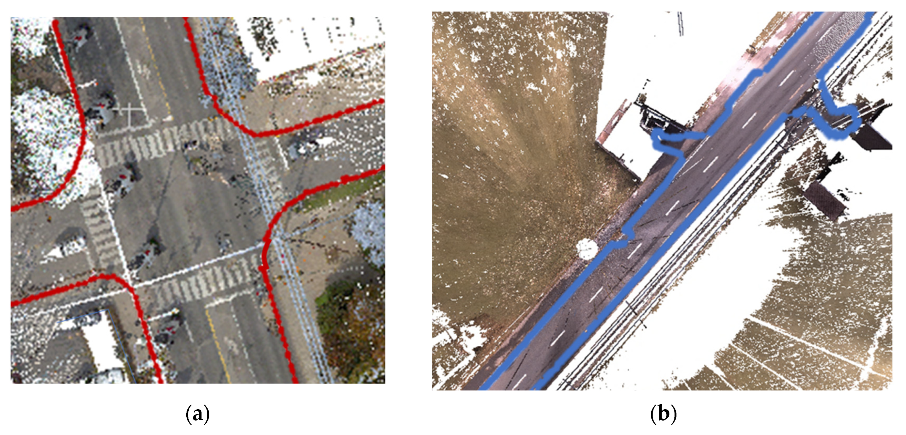
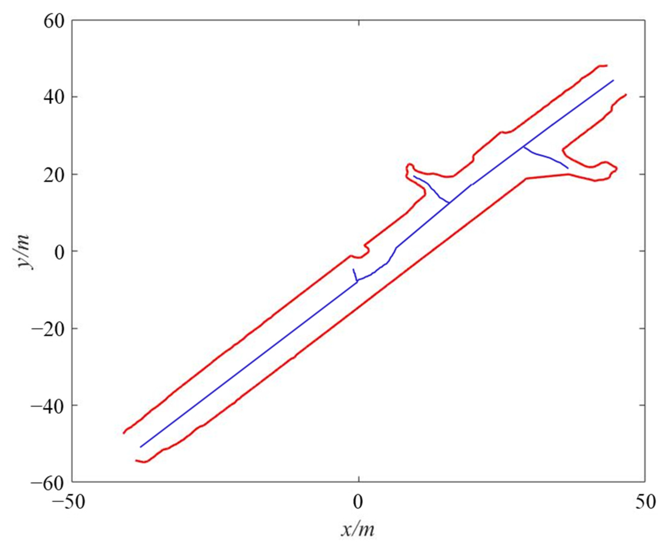
Considering the road scenarios L002 in Toronto-3D and sg27_1 in Semantic3D as examples, the alpha-shape method is first applied to extract the road boundary when α is defined as 1 m (see Figure 7).
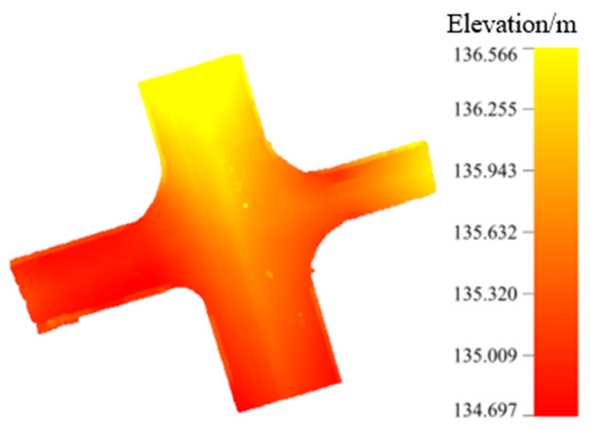
To accurately obtain the elevation of the entire intersection, the DEM is constructed by the interpolation method based on the uniformly distributed point set. The generated point set and DEM are shown in Figure 8 and Figure 9.
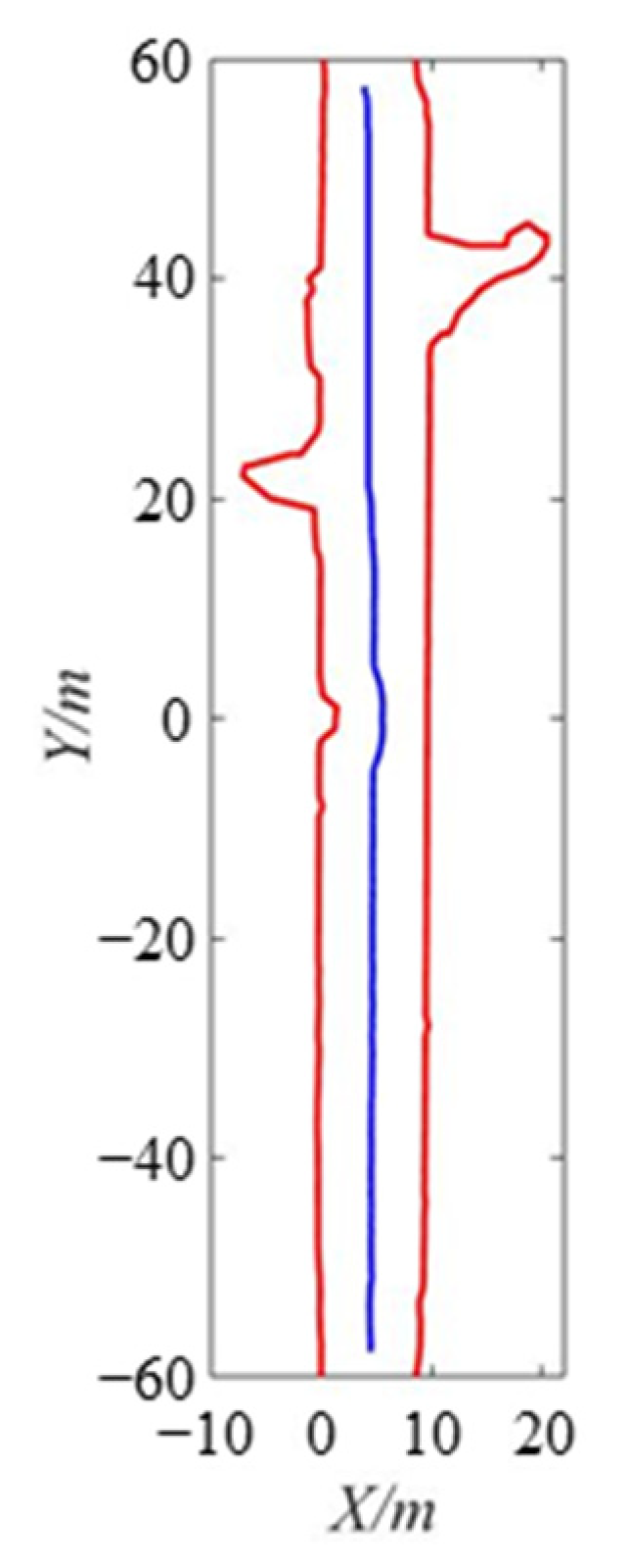
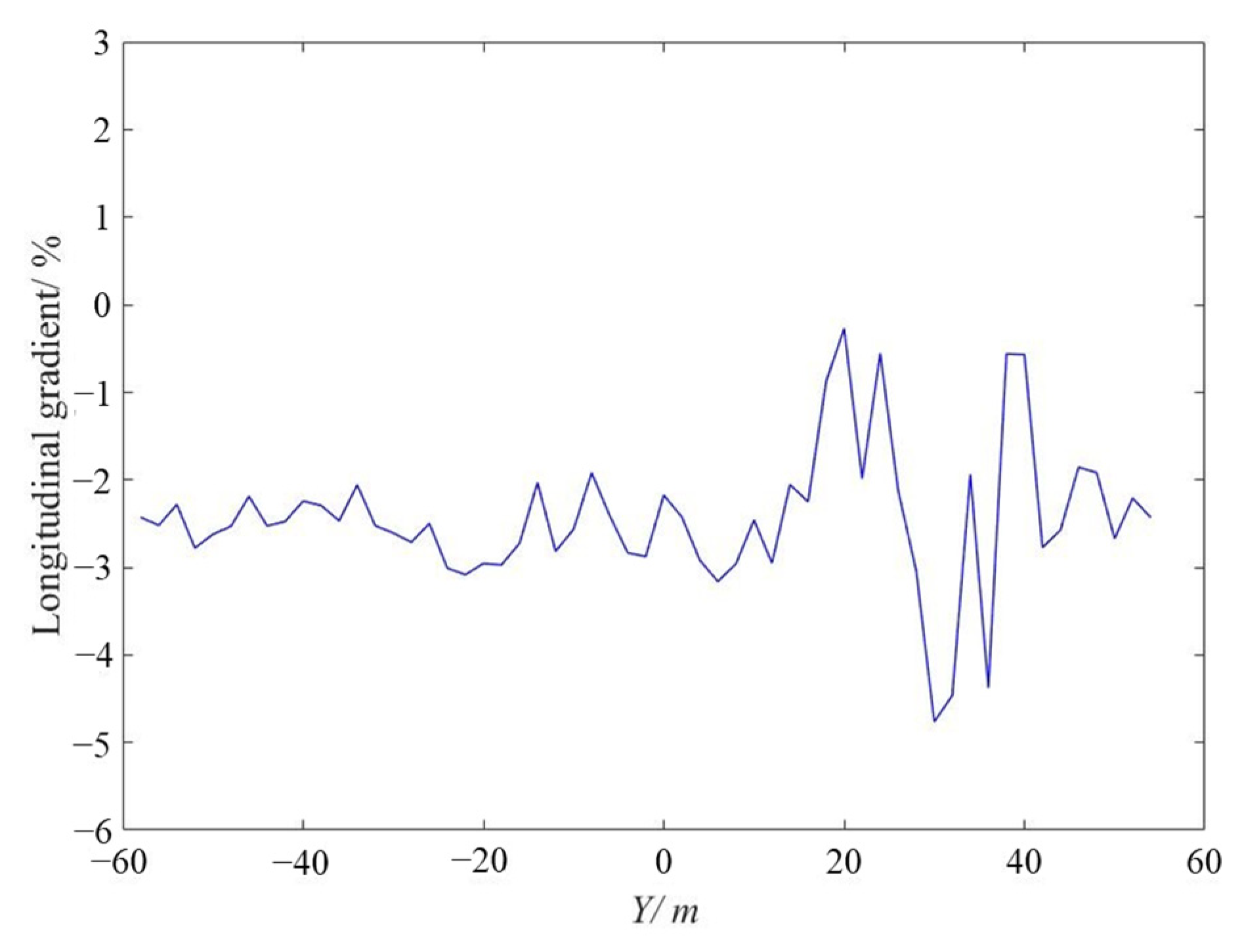
Thereafter, the Voronoi diagram method is used to obtain the centerline. To ensure the accuracy of extraction, the extraneous lines are removed based on the number of line segments (set as 25) in side branches through several iterations (see Figure 10). The original surface points are converted based on the centerline of the main road. The transformed boundary and centerline are presented in Figure 11. Meanwhile, the longitudinal slope is obtained from the elevation of the centerline expressed by Equation (8). As illustrated in Figure 12, the mean longitudinal slope of the road is −2.3%.
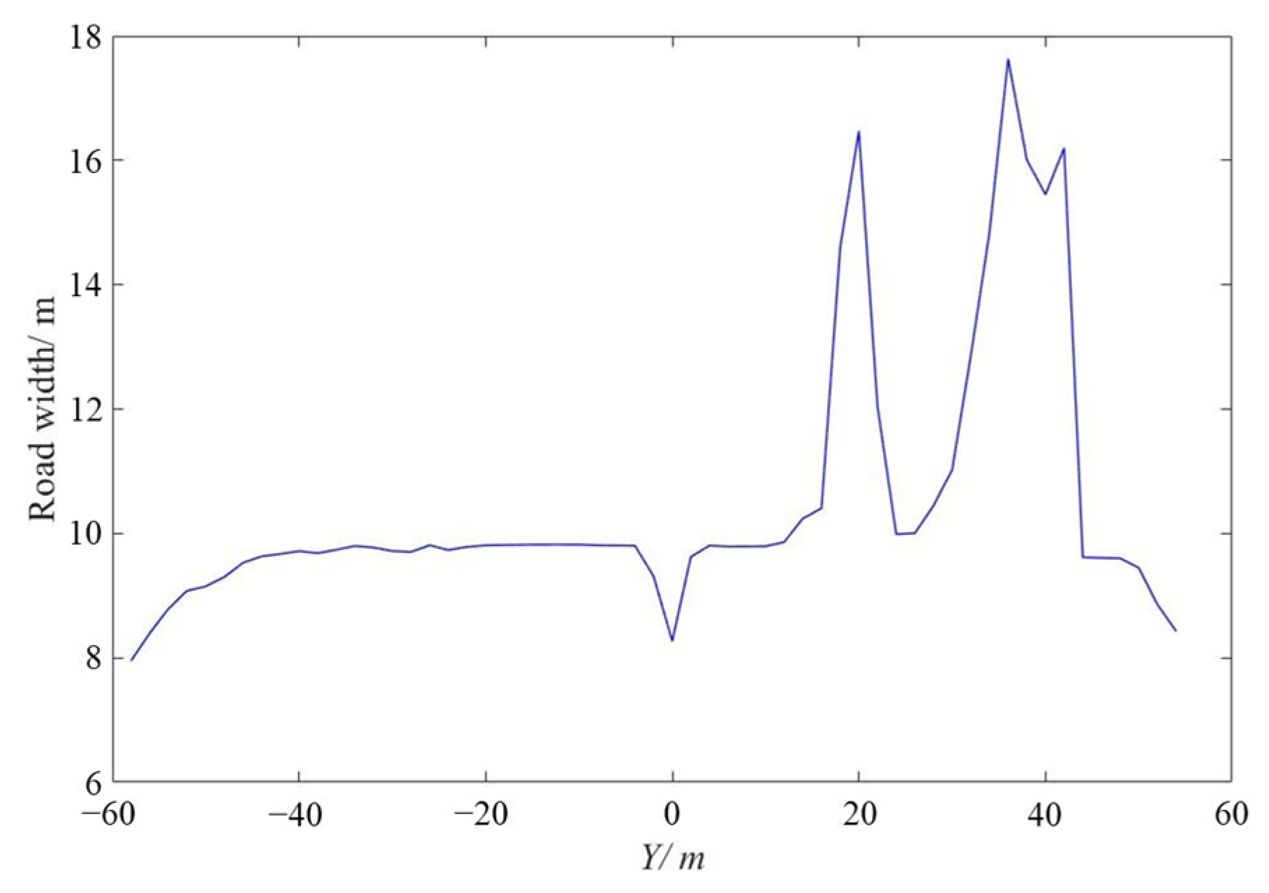
In addition, the road width is calculated as the difference between the left and right sides (see Figure 13). As depicted in this figure, apparent road widening occurs at 20 m and 40 m because of the crossings. The cross-sectional profiles on both sides are fitted. The results are shown in Figure 14. As illustrated in this figure, the left and right cross slopes are 2.2 % and 2.3 % on average, respectively.
To verify the reliability and accuracy of the geometric information extraction, manual measurement was employed in CloudCompare software to manually segment and measure the slices of cross-sections every 2 m. Certain coordinate information can be displayed by visualization in CloudCompare software during the measurement process. The highest point of the cross-section (painted with the darkest red) is the midpoint of the road, owing to the form of the cross-section. For each cross-section, the left, right, and midpoint points could be selected to be exported in a batch and to calculate the left and right cross slopes (see Figure 15). The maximum and mean absolute errors of geometric information between the extracted methods and manual measurements are as shown in Table 3.
Table 3 demonstrates that the mean absolute error of road width between the extracted methods and manual measurements is less than 0.0094 m. Furthermore, the mean absolute errors for the other geometric information are less than 0.0091%. These indicate that the extracted methods are accurate and effective. The maximum and mean absolute errors for road width are larger than those for longitudinal gradient and cross slope. Based on the location of the maximum absolute error, we analyze the errors of geometric information from 20 to 40 m on the Y-coordinate to further investigate the cause of the larger errors. The comparison between the extracted and manually measured geometric information is presented in Table 4.
As shown in Table 4, the errors for different geometric information are larger when the Y-coordinates are 20 m and 30–36 m. Combined with the horizontal alignment, it can be observed that intersections exist in this range. This affects the surface segmentation. This directly results in the larger error of the road width, and further reduces the extraction accuracy of the geometric information.

3.4. Digital Modeling in BIM Environment

The 3D road scenario of sg27_1 is established using the proposed digital modeling process in Section 2.5. The road scenario consists of the road entity model, infrastructure components, and other detailed designs. Among these, the process of establishing the road entity model should be given attention because of the road geometric information. More specifically, the road route is first interpolated to generate a series of interpolation points. Thereafter, these points are assessed and grouped to place the designed adaptive components. This establishes a road entity model. In this case study, the road alignment is straight, and the road width is approximately 10 m. Hence, 5% of the width is considered as the threshold value. Two interpolation points are grouped as the origin and destination of the adaptive road component. Subsequently, the placements of different infrastructures are determined based on boundary curves. The infrastructure components are manually placed and generated through Revit software. The surrounding vegetation and other elements are manually constructed based on the imported point clouds. The road entity is applied in the material of bituminous concrete. The established digital road scenario is compared with the LiDAR data (see Figure 16).
As shown in Figure 16, the road entity and infrastructure essentially achieve correspondences in the digital road scenarios. However, there are differences in the vegetation models because of the missing point clouds and different modeling approaches. Specifically, the morphology of low vegetation is incomplete owing to the occlusion of other objects and the larger distance from the sensor during point cloud collection. Although the surrounding vegetation can be effectively divided by the semantic segmentation network, these fail to be completely modeled with regard to the shapes and poses. Meanwhile, the vegetation is in the block distribution with denser locations. This cannot be sequentially realized by the modeling. Therefore, there is scope for improvement through multi-view images and the spatial geometry information of point clouds. It is likely to be feasible to accurately and completely model the surrounding vegetation.

4. Discussion

The results in Section 3 demonstrate the proposed framework can achieve the objective and make contributions, as shown in Section 1. First, the improved SCF-Net segments different categories of objects in road scenarios that can easily extract the geometric information and establish semantic-rich digital models. The quantitative results and visualizations show the improved SCF-Net is beneficial to enhance the segmentation performance in large-scale point cloud benchmarks. However, it can be argued that road markings, low vegetation, and infrastructure categories could not be identified because of missing points and indistinct geometric structures. Hence, a future direction for this research will be motivated by extracting more features and structures from point clouds or multiple data sources, such as optical images, GIS databases, and vehicle trajectory.
Second, a series of methods that extract the geometric information from point clouds of the segmented road surface is proposed. The mean absolute errors between the extracted and manually measured geometric information verify the reliability and accuracy of the extraction methods. Furthermore, Dynamo and Revit software are expected to generate digital models of the road entities and infrastructures based on the obtained semantic and geometric information. The nodes in Dynamo are used to import the data and establish the model. Nevertheless, the process of digital modeling is semi-automated. Manual modeling is required based on the imported point clouds for surrounding vegetation and other elements. Therefore, full automation is a future objective for digital modeling from LiDAR data of road scenarios.

5. Conclusions

In this study, an improved semantic segmentation network was used to divide the road surface and other infrastructures. The alpha-shape and Voronoi diagram methods were applied to extract the road boundary and centerline, and thereby obtain road geometric information. Subsequently, the road entity model and infrastructure components were constructed through Dynamo and Revit software. Finally, a digital road scenario was developed. The following conclusions could be drawn:
(1) The improved networks were validated by experiments on the large-scale point cloud benchmarks Toronto-3D and Semantic3D. The results of semantic segmentation showed that the OA of our net on the two datasets were 95.3 and 95.0%, respectively. Meanwhile, road surface achieved a better performance (IoU of 95.7 and 97.9%) than the other categories. This demonstrated that the proposed net is accurate and effective.
(2) Compared with the extracted and manually measured geometric information in CloudCompare software, the mean absolute error for road width was less than 0.0094 m, and those for the other geometric information were less than 0.0091%. Therefore, the extraction methods were effective for calculating the geometric information.
(3) The road entity and infrastructure modeling in BIM was established based on Dynamo and Revit software. This achieved correspondence in the digital road scenarios and LiDAR data.
This proposed framework is expected to provide transportation agencies with a workflow for updating the semantic and geomatic information of as-built roads and surrounding infrastructure as LiDAR technology and BIM technology become more common. It could also provide accurate descriptions for as-built road and infrastructure features, which extends beyond helping enhance the efficiency of inventorying to a potential reference in asset management and road safety inspection. Meanwhile, our study focused on the acquired data rather than the laser scanner system. It selected 3D coordinates and RGB information to represent the point clouds. This increased the applicability and portability of the proposed methods. In addition, the proposed methods could be combined with other data sources to accomplish road marking extraction and object recognition.
Finally, this study only demonstrated the applicability and accuracy of the proposed methods from the perspective of theoretical and manual measurements. Further field experiments are required to conduct geometric information extraction and validate its accuracy.

Author Contributions

Conceptualization, Y.W.; Data curation, S.W.; Formal analysis, J.L.; Funding acquisition, B.Y.; Investigation, Y.W. and B.Y.; Methodology, Y.W.; Software, J.L.; Supervision, B.Y.; Validation, T.C.; Writing—original draft, Y.W.; Writing—review and editing, W.W. and B.Y.; Supervision, B.Y. and X.Q. All authors have read and agreed to the published version of the manuscript.

Funding

This study was supported by the projects found by the National Natural Science Foundation of China under Grants 51878039 and 52078034, National Key R&D Program of China under Grants 2017YFF0205600 and Jiangsu transportation science and technology project under Grants 2020Y19-1(1), to which the authors are very grateful.

Data Availability Statement

The data used to support the findings of this study are available from the corresponding author upon request.

Acknowledgments

The authors would like to thank the Jiangsu transportation science and technology project for the Open Access Funding.

Conflicts of Interest

The authors declare no conflict of interest.

References

  1. Jiang, F.; Ma, L.; Broyd, T.; Chen, W.; Luo, H. Building Digital Twins of Existing Highways Using Map Data Based on Engineering Expertise. Autom. Constr. 2022, 134, 104081. [Google Scholar] [CrossRef]
  2. Jalayer, M.; Gong, J.; Zhou, H.; Grinter, M. Evaluation of Remote Sensing Technologies for Collecting Roadside Feature Data to Support Highway Safety Manual Implementation. J. Transp. Saf. Secur. 2015, 7, 345–357. [Google Scholar] [CrossRef]
  3. Vaiana, R.; Perri, G.; Iuele, T.; Gallelli, V. A Comprehensive Approach Combining Regulatory Procedures and Accident Data Analysis for Road Safety Management Based on the European Directive 2019/1936/Ec. Safety 2021, 7, 6. [Google Scholar] [CrossRef]
  4. Hou, Q.; Ai, C. A Network-Level Sidewalk Inventory Method Using Mobile LiDAR and Deep Learning. Transp. Res. Part C Emerg. Technol. 2020, 119, 102772. [Google Scholar] [CrossRef]
  5. Holgado-Barco, A.; González-Aguilera, D.; Arias-Sanchez, P.; Martinez-Sanchez, J. Semiautomatic Extraction of Road Horizontal Alignment from a Mobile LiDAR System. Comput.-Aided Civ. Infrastruct. Eng. 2015, 30, 217–228. [Google Scholar] [CrossRef]
  6. Gu, H.; Han, Y.; Yang, Y.; Li, H.; Liu, Z.; Soergel, U.; Blaschke, T.; Cui, S. An Efficient Parallel Multi-Scale Segmentation Method for Remote Sensing Imagery. Remote Sens. 2018, 10, 590. [Google Scholar] [CrossRef] [Green Version]
  7. Holgado-Barco, A.; Riveiro, B.; González-Aguilera, D.; Arias, P. Automatic Inventory of Road Cross-Sections from Mobile Laser Scanning System. Comput.-Aided Civ. Infrastruct. Eng. 2017, 32, 3–17. [Google Scholar] [CrossRef]
  8. Qiu, S.; Anwar, S.; Barnes, N. Semantic Segmentation for Real Point Cloud Scenes via Bilateral Augmentation and Adaptive Fusion. In Proceedings of the IEEE Computer Society Conference on Computer Vision and Pattern Recognition, Nashville, TN, USA, 20–25 June 2021; pp. 1757–1767. [Google Scholar]
  9. Lin, Y.; Vosselman, G.; Cao, Y.; Yang, M.Y. Active and Incremental Learning for Semantic ALS Point Cloud Segmentation. ISPRS J. Photogramm. Remote Sens. 2020, 169, 73–92. [Google Scholar] [CrossRef]
  10. Pierdicca, R.; Paolanti, M.; Matrone, F.; Martini, M.; Morbidoni, C.; Malinverni, E.S.; Frontoni, E.; Lingua, A.M. Point Cloud Semantic Segmentation Using a Deep Learning Framework for Cultural Heritage. Remote Sens. 2020, 12, 1005. [Google Scholar] [CrossRef] [Green Version]
  11. Han, X.; Dong, Z.; Yang, B. A Point-Based Deep Learning Network for Semantic Segmentation of MLS Point Clouds. ISPRS ISPRS J. Photogramm. Remote Sens. 2021, 175, 199–214. [Google Scholar] [CrossRef]
  12. Rodríguez-Cuenca, B.; García-Cortés, S.; Ordóñez, C.; Alonso, M.C. An Approach to Detect and Delineate Street Curbs from MLS 3D Point Cloud Data. Autom. Constr. 2015, 51, 103–112. [Google Scholar] [CrossRef]
  13. Ibrahim, S.; Lichti, D. Curb-Based Street Floor Extraction From Mobile Terrestrial Lidar Point Cloud. ISPRS-Int. Arch. Photogramm. Remote Sens. Spat. Inf. Sci. 2012, XXXIX-B5, 193–198. [Google Scholar] [CrossRef] [Green Version]
  14. Xu, S.; Wang, R.; Zheng, H. Road Curb Extraction from Mobile LiDAR Point Clouds. IEEE Trans. Geosci. Remote Sens. 2017, 55, 996–1009. [Google Scholar] [CrossRef] [Green Version]
  15. Kumar, P.; McElhinney, C.P.; Lewis, P.; McCarthy, T. An Automated Algorithm for Extracting Road Edges from Terrestrial Mobile LiDAR Data. ISPRS J. Photogramm. Remote Sens. 2013, 85, 44–55. [Google Scholar] [CrossRef] [Green Version]
  16. Kumar, P.; Lewis, P.; McCarthy, T. The Potential of Active Contour Models in Extracting Road Edges from Mobile Laser Scanning Data. Infrastructures 2017, 2, 9. [Google Scholar] [CrossRef] [Green Version]
  17. Guo, J.; Tsai, M.J.; Han, J.Y. Automatic Reconstruction of Road Surface Features by Using Terrestrial Mobile Lidar. Autom. Constr. 2015, 58, 165–175. [Google Scholar] [CrossRef]
  18. Yadav, M.; Singh, A.K.; Lohani, B. Extraction of Road Surface from Mobile LiDAR Data of Complex Road Environment. Int. J. Remote Sens. 2017, 38, 4645–4672. [Google Scholar] [CrossRef]
  19. Guo, Y.; Wang, H.; Hu, Q.; Liu, H.; Liu, L.; Bennamoun, M. Deep Learning for 3D Point Clouds: A Survey. IEEE Trans. Pattern. Anal. Mach. Intell. 2021, 43, 4338–4364. [Google Scholar] [CrossRef]
  20. Lawin, F.J.; Danelljan, M.; Tosteberg, P.; Bhat, G.; Khan, F.S.; Felsberg, M. Deep Projective 3D Semantic Segmentation. Lect. Notes Comput. Sci. 2017, 10424 LNCS, 95–107. [Google Scholar]
  21. Tchapmi, L.; Choy, C.; Armeni, I.; Gwak, J.; Savarese, S. SEGCloud: Semantic Segmentation of 3D Point Clouds. In Proceedings of the 2017 International Conference on 3D Vision, (3DV), Qingdao, China, 10–12 October 2017; pp. 537–547. [Google Scholar]
  22. Graham, B.; Engelcke, M.; Van Der Maaten, L. 3D Semantic Segmentation with Submanifold Sparse Convolutional Networks. In Proceedings of the IEEE Computer Society Conference on Computer Vision and Pattern Recognition, Salt Lake City, UT, USA, 18–23 June 2018; pp. 9224–9232. [Google Scholar]
  23. Meng, H.Y.; Gao, L.; Lai, Y.K.; Manocha, D. VV-Net: Voxel VAE Net with Group Convolutions for Point Cloud Segmentation. In Proceedings of the IEEE International Conference on Computer Vision 2019, Seoul, Republic of Korea, 27 October–2 November 2019; pp. 8499–8507. [Google Scholar]
  24. Sha, A.; Yun, D.; Hu, L.; Tang, C. Influence of Sampling Interval and Evaluation Area on the Three-Dimensional Pavement Parameters. Road Mater. Pavement Des. 2021, 22, 1964–1985. [Google Scholar] [CrossRef]
  25. Jing, H.; You, S. Point Cloud Labeling Using 3D Convolutional Neural Network. In Proceedings of the International Conference on Pattern Recognition, Cancun, Mexico, 4–8 December 2016; pp. 2670–2675. [Google Scholar]
  26. Hu, Q.; Yang, B.; Xie, L.; Rosa, S.; Guo, Y.; Wang, Z.; Trigoni, N.; Markham, A. Learning Semantic Segmentation of Large-Scale Point Clouds With Random Sampling. IEEE Trans. Pattern Anal. Mach. Intell. 2021, 44, 1. [Google Scholar] [CrossRef]
  27. Fan, S.Q.; Dong, Q.L.; Zhu, F.H.; Lv, Y.S.; Ye, P.J.; Wang, F.Y.; Ieee Comp, S.O.C. SCF-Net: Learning Spatial Contextual Features for Large-Scale Point Cloud Segmentation. In Proceedings of the IEEE/CVF Conference on Computer Vision and Pattern Recognition (CVPR), Nashville, TN, USA, 20–25 June 2021; pp. 14499–14508. [Google Scholar]
  28. Yang, X.; Tang, L.; Niu, L.; Zhang, X.; Li, Q. Generating Lane-Based Intersection Maps from Crowdsourcing Big Trace Data. Transp. Res. Part C Emerg. Technol. 2018, 89, 168–187. [Google Scholar] [CrossRef]
  29. Zhang, Z.; Li, J.; Guo, Y.; Yang, C.; Wang, C. 3D Highway Curve Reconstruction from Mobile Laser Scanning Point Clouds. IEEE Trans. Intell. Transp. Syst. 2020, 21, 4762–4772. [Google Scholar] [CrossRef]
  30. Strygulec, S.; Muller, D.; Meuter, M.; Nunn, C.; Ghosh, S.; Wohler, C. Road Boundary Detection and Tracking Using Monochrome Camera Images. In Proceedings of the 16th International Conference on Information Fusion, (FUSION 2013), Istanbul, Turkey, 9–12 July 2013; pp. 864–870. [Google Scholar]
  31. Mi, X.; Yang, B.; Dong, Z.; Chen, C.; Gu, J. Automated 3D Road Boundary Extraction and Vectorization Using MLS Point Clouds. IEEE Trans. Intell. Transp. Syst. 2022, 23, 5287–5297. [Google Scholar] [CrossRef]
  32. Di Mascio, P.; Di Vito, M.; Loprencipe, G.; Ragnoli, A. Procedure to Determine the Geometry of Road Alignment Using GPS Data. Procedia Soc. Behav. Sci. 2012, 53, 1202–1215. [Google Scholar] [CrossRef] [Green Version]
  33. Justo, A.; Soilán, M.; Sánchez-Rodríguez, A.; Riveiro, B. Scan-to-BIM for the Infrastructure Domain: Generation of IFC-Complaint Models of Road Infrastructure Assets and Semantics Using 3D Point Cloud Data. Autom. Constr. 2021, 127, 13. [Google Scholar] [CrossRef]
  34. Soilán, M.; Justo, A.; Sánchez-Rodríguez, A.; Riveiro, B. 3D Point Cloud to BIM: Semi-Automated Framework to Define IFC Alignment Entities from MLS-Acquired LiDAR Data of Highway Roads. Remote Sens. 2020, 12, 2301. [Google Scholar] [CrossRef]
  35. Tang, F.; Ma, T.; Zhang, J.; Guan, Y.; Chen, L. Integrating Three-Dimensional Road Design and Pavement Structure Analysis Based on BIM. Autom. Constr. 2020, 113, 17. [Google Scholar] [CrossRef]
  36. Soilan, M.; Sanchez-Rodriguez, A.; del Rio-Barral, P.; Perez-Collazo, C.; Arias, P.; Riveiro, B. Review of Laser Scanning Technologies and Their Applications for Road and Railway Infrastructure Monitoring. Infrastructures 2019, 4, 58. [Google Scholar] [CrossRef] [Green Version]
  37. Olsen, M.J.; Kuester, F.; Chang, B.J.; Hutchinson, T.C. Terrestrial Laser Scanning-Based Structural Damage Assessment. J. Comput. Civ. Eng. 2010, 24, 264–272. [Google Scholar] [CrossRef]
  38. Kukko, A.; Kaartinen, H.; Hyyppa, J.; Chen, Y.W. Multiplatform Mobile Laser Scanning: Usability and Performance. Sensors 2012, 12, 11712–11733. [Google Scholar] [CrossRef]
  39. Jaakkola, A.; Hyyppa, J.; Hyyppa, H.; Kukko, A. Retrieval Algorithms for Road Surface Modelling Using Laser-Based Mobile Mapping. Sensors 2008, 8, 5238–5249. [Google Scholar] [CrossRef] [PubMed] [Green Version]
  40. Zhang, C.; Xu, S.; Jiang, T.; Liu, J.; Liu, Z.; Luo, A.; Ma, Y. Integrating Normal Vector Features into an Atrous Convolution Residual Network for Lidar Point Cloud Classification. Remote Sens. 2021, 13, 3427. [Google Scholar] [CrossRef]
  41. Fang, L.; Shen, G.; You, Z.; Guo, Y.; Fu, H.; Zhao, Z.; Chen, C. A Joint Network of Point Cloud and Multiple Views for Roadside Objects Recognition from Mobile Laser Point Clouds. Cehui Xuebao/Acta Geod. Cartogr. Sin. 2021, 50, 1558–1573. [Google Scholar] [CrossRef]
  42. AlHajri, M.F.; El-Hawary, M.E. Exploiting the Radial Distribution Structure in Developing a Fast and Flexible Radial Power Flow for Unbalanced Three-Phase Networks. IEEE Trans. Power Deliv. 2010, 25, 378–389. [Google Scholar] [CrossRef]
  43. Guan, H.Y.; Li, J.; Yu, Y.T.; Chapman, M.; Wang, C. Automated Road Information Extraction From Mobile Laser Scanning Data. IEEE Trans. Intell. Transp. Syst. 2015, 16, 194–205. [Google Scholar] [CrossRef]
  44. Ma, Y.; Easa, S.; Cheng, J.C.A.; Yu, B. Automatic Framework for Detecting Obstacles Restricting 3D Highway Sight Distance Using Mobile Laser Scanning Data. J. Comput. Civ. Eng. 2021, 35, 19. [Google Scholar] [CrossRef]
  45. Al-Tamimi, M.S.H.; Sulong, G.; Shuaib, I.L. Alpha Shape Theory for 3D Visualization and Volumetric Measurement of Brain Tumor Progression Using Magnetic Resonance Images. Magn. Reson. Imaging 2015, 33, 787–803. [Google Scholar] [CrossRef]
  46. Widyaningrum, E.; Peters, R.Y.; Lindenbergh, R.C. Building Outline Extraction from ALS Point Clouds Using Medial Axis Transform Descriptors. Pattern Recognit. 2020, 106, 15. [Google Scholar] [CrossRef]
  47. Tejenaki, S.A.K.; Ebadi, H.; Mohammadzadeh, A. A New Hierarchical Method for Automatic Road Centerline Extraction in Urban Areas Using LIDAR Data. Adv. Space Res. 2019, 64, 1792–1806. [Google Scholar] [CrossRef]
  48. Younas, S.; Figley, C.R. Development, Implementation and Validation of an Automatic Centerline Extraction Algorithm for Complex 3D Objects. J. Med. Biol. Eng. 2019, 39, 184–204. [Google Scholar] [CrossRef]
  49. Tan, W.K.; Qin, N.N.; Ma, L.F.; Li, Y.; Du, J.; Cai, G.R.; Yang, K.; Li, J.; Ieee Comp, S.O.C. Toronto-3D: A Large-Scale Mobile LiDAR Dataset for Semantic Segmentation of Urban Roadways. In Proceedings of the IEEE/CVF Conference on Computer Vision and Pattern Recognition (CVPR), Seattle, WA, USA, 13–19 June 2020; pp. 797–806. [Google Scholar]
  50. Hackel, T.; Wegner, J.D.; Savinov, N.; Ladicky, L.; Schindler, K.; Pollefeys, M. Large-Scale Supervised Learning For 3D Point Cloud Labeling: Semantic3d.Net. Photogramm. Eng. Remote Sens. 2018, 84, 297–308. [Google Scholar] [CrossRef]
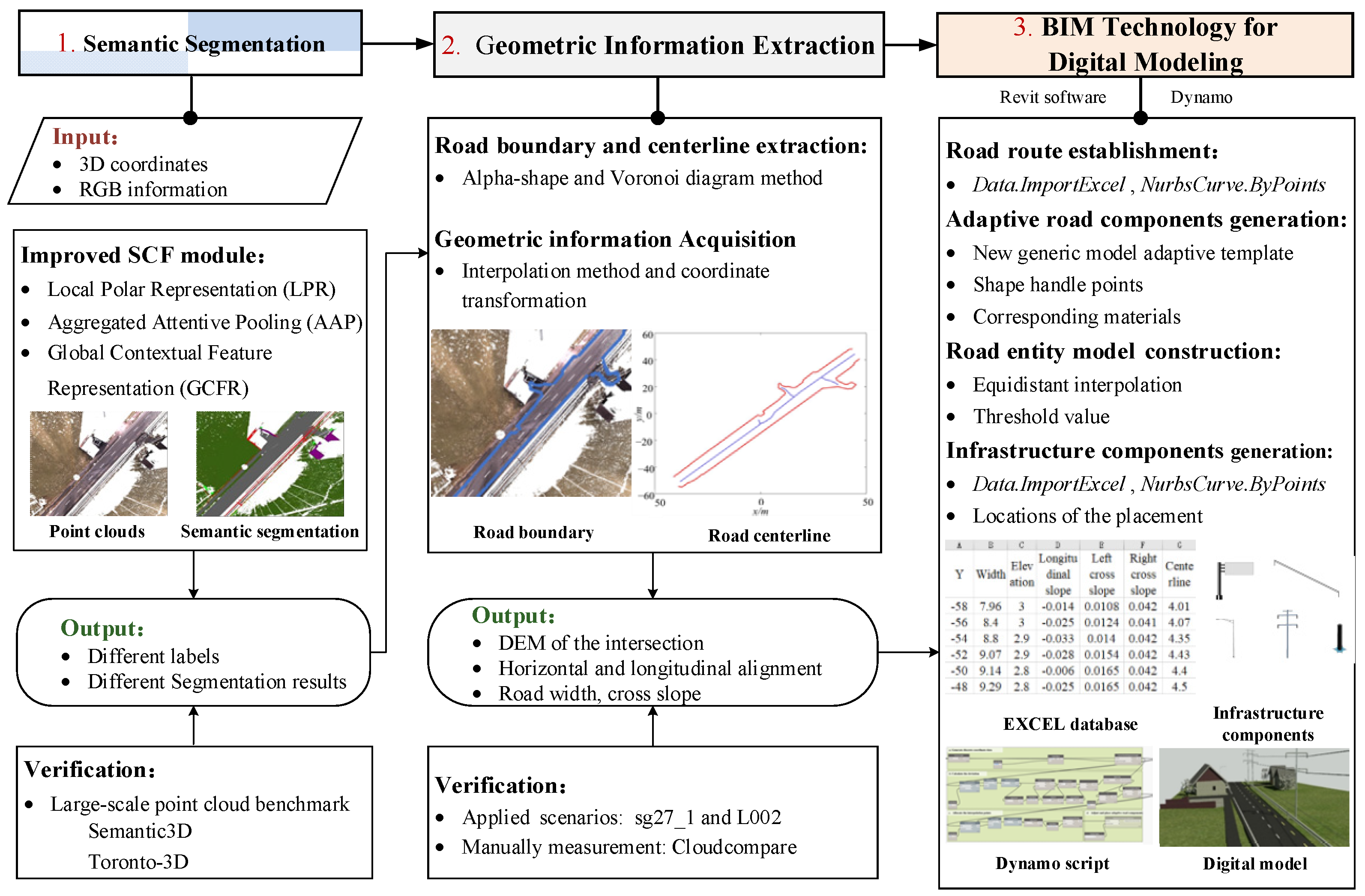
Figure 1. Workflow of the methods.
Remotesensing 15 00576 g001
Figure 2. Improved SCF module.
Remotesensing 15 00576 g002
Figure 3. Architecture of improved SCF-Net.
Remotesensing 15 00576 g003
Figure 4. Setting of adaptive road components.
Remotesensing 15 00576 g004
Figure 5. Comparison between colored point clouds and predicted segmentation results (Toronto-3D).
Remotesensing 15 00576 g005
Figure 6. Comparison between colored point clouds and predicted segmentation results (Semantic3D).
Remotesensing 15 00576 g006
Figure 7. Extraction of the road boundary. (a) Intersection; (b) road.
Remotesensing 15 00576 g007
Figure 8. Generated point set.
Remotesensing 15 00576 g008
Figure 9. Generated DEM.
Remotesensing 15 00576 g009
Figure 10. Generated original centerline.
Remotesensing 15 00576 g010
Figure 11. Transformed boundary and centerline of the main road.
Remotesensing 15 00576 g011
Figure 12. Longitudinal gradient.
Remotesensing 15 00576 g012
Figure 13. Road width.
Remotesensing 15 00576 g013
Figure 14. Cross slopes of the road. (a) Left cross slope; (b) right cross slope.
Remotesensing 15 00576 g014
Figure 15. Manual measurement of the geometric information.
Remotesensing 15 00576 g015
Figure 16. Comparison of LiDAR data and the digital road scenario.
Remotesensing 15 00576 g016
Table 1. Semantic segmentation (L002) results of Toronto-3D dataset %.
MethodmIoU
(%)
OA
(%)
IoU (%)
Road SurfaceRoad Mrk.Natural.BuildingUtil. LinePoleCarFence
Pointnet++65.093.093.919.490.581.768.562.958.944.4
RandLA-Net74.388.487.422.096.492.785.975.586.647.6
SCF-Net71.593.591.419.690.987.378.572.684.647.4
Ours73.995.395.725.994.086.381.571.878.158.1
Table 2. Semantic segmentation (semantic-8) results of Semantic3D Dataset %.
MethodmIoU
(%)
OA
(%)
IoU (%)
Road SurfaceNatural. High Veg.Low Veg.BuildingInfrastructureScanning Art.Cars
Pointnet++63.185.781.978.164.351.775.936.443.772.6
RandLA-Net71.894.29688.665.362.095.949.827.889.3
Ours74.795.097.994.170.864.394.048.538.889.2
Table 3. Error Between Extraction Methods and Manual Measurement.
IndicatorsGeometric Information
Road Width/mLongitudinal
Gradient/%
Cross Slope
Left Cross Slope/%Right Cross Slope/%
Mean absolute error0.00940.00910.00740.0073
Maximum absolute error0.05300.04750.02380.0237
Location of Maximum absolute error/m 36302020
Table 4. Comparison between extracted and manually measured geometric information.
Location/mRoad Width/mLongitudinal Gradient/%
Extracted MethodsManual
Measurement
Absolute ErrorExtracted
Methods
Manual
Measurement
Absolute Error
2016.472316.4228 0.0495 −0.2728 −0.2700 0.0028
2212.046812.0348 0.0121 −1.9862 −1.9663 0.0199
249.99019.9931 0.0030 −0.5564 −0.5553 0.0011
2610.00439.9944 0.0100 −2.1261 −2.1304 0.0043
2810.448010.4376 0.0104 −3.0431 −3.0431 0.0000
3011.025111.0140 0.0110 −4.7629 −4.8104 0.0475
3212.857012.8312 0.0257 −4.4626 −4.5072 0.0446
3414.842914.8132 0.0297 −1.9402 −1.9594 0.0192
3617.633117.5801 0.0530 −4.3765 −4.4198 0.0433
3816.009215.9611 0.0481 −0.5631 −0.5687 0.0056
4015.450515.4195 0.0310 −0.5698 −0.5641 0.0057
Location/mLeft cross slope/%Right cross slope/%
Extracted methodsManual measurementAbsolute errorExtracted methodsManual measurementAbsolute error
202.09602.11980.02382.09042.11410.0237
222.14362.16610.02252.02532.04650.0212
242.16282.15820.00461.84971.84570.0040
262.27892.27550.00341.70421.70170.0025
282.44852.44970.00121.65681.65770.0009
302.45042.42710.02331.81621.79890.0173
322.56082.53770.02311.70561.69020.0154
342.32592.30470.02122.16792.14820.0197
362.18692.16800.01892.20002.18100.0190
382.23012.21080.01932.30622.28630.0199
402.02452.04650.02201.42231.43780.0155
Disclaimer/Publisher’s Note: The statements, opinions and data contained in all publications are solely those of the individual author(s) and contributor(s) and not of MDPI and/or the editor(s). MDPI and/or the editor(s) disclaim responsibility for any injury to people or property resulting from any ideas, methods, instructions or products referred to in the content.