High-Resolution SAR Imaging with Azimuth Missing Data Based on Sub-Echo Segmentation and Reconstruction

Abstract

Due to the substantial electromagnetic interference, radar interruptions, and other factors, the SAR system may fail to receive valid data in some azimuth areas. This phenomenon is known as Azimuth Missing Data (AMD). If classical SAR imaging algorithms are performed directly using AMD echo, the imaging results may be defocused or even display false targets, which seriously affects the accuracy of the image. Thus, we proposed a Sub-echo Segmentation and Reconstruction Azimuth Missing Data SAR Imaging Algorithm (SSR-AMDIA) to solve the problem of incomplete echo SAR imaging in this article. Instead of using the motion compensation step of the Polar Format algorithm (PFA) to recover the full echo from the AMD echo, the proposed SSR-AMDIA eliminates the effect of the planar approximation in PFA and expands the maximum depth of focus (DOF). The raw AMD echo was first subjected to range compression and Range Cell Migration Correction (RCMC), after which the AMD-RCMC echo was divided along the range direction. Then, we constructed a series of phase compensation functions based on the sub-segment AMD-RCMC echoes to guarantee the perfect recovery of the full RCMC echoes corresponding to the sub-scenes. Finally, we combined them to obtain the complete RCMC echo, and an excellent focused imaging result was then obtained via azimuth compression. Simulation and experimental data verified the effectiveness of the proposed algorithm. Furthermore, we derived the mathematical expressions for the two-dimensional maximum DOFs of the proposed algorithm. In contrast to the State-Of-the-Art (SOA) AMDIA, the SSR-AMDIA can obtain a superior imaging performance in a larger imaging scope under the conditions of most AMD cases.

1. Introduction

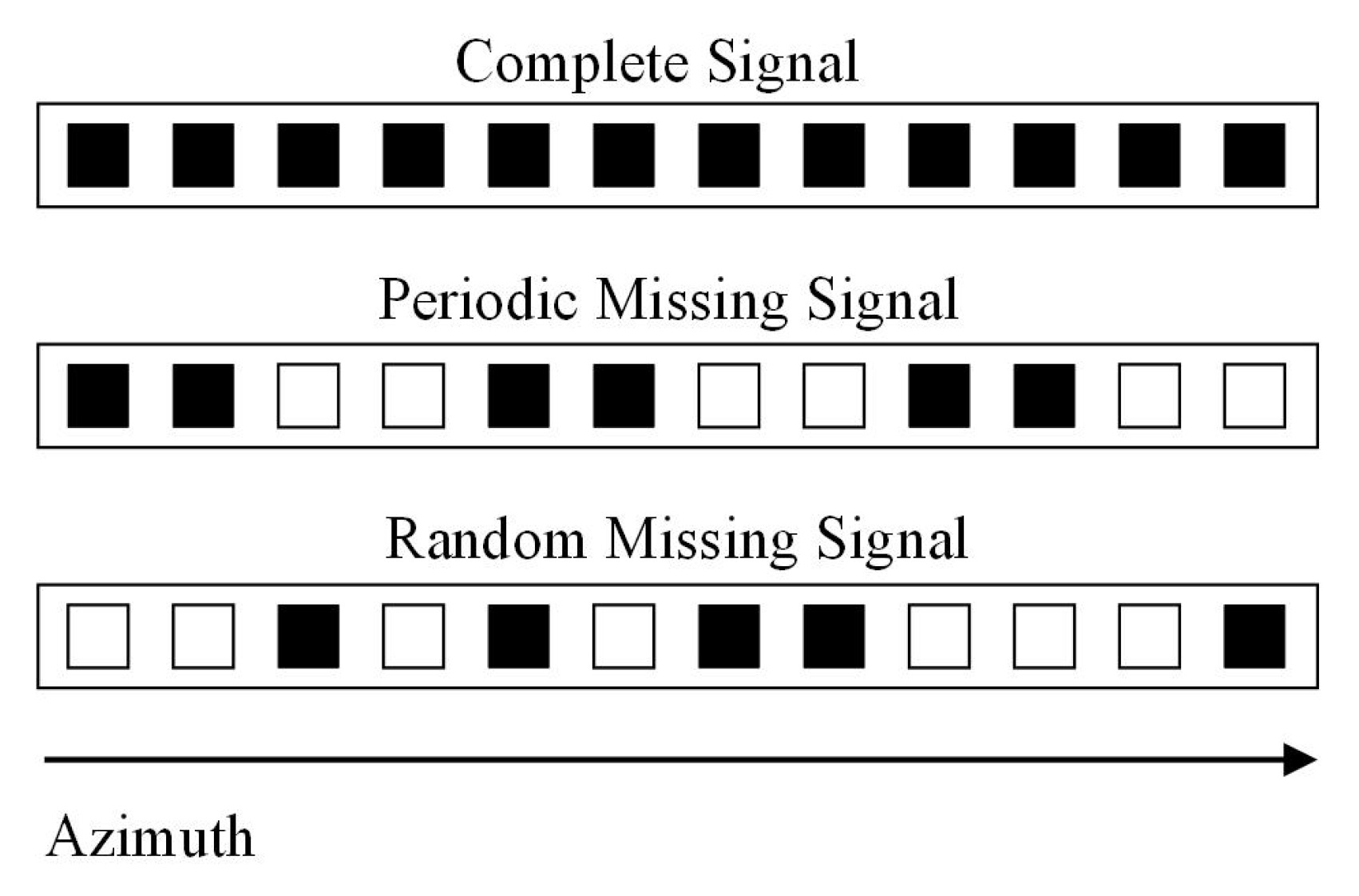
Unavoidable interference between SAR systems and imaging scenes, interruptions in SAR systems for different purposes, or new SAR mission requirements will result in the azimuth missing data (AMD) [1,2]. If the conventional SAR imaging algorithm is used directly in the AMD echo case, false targets or severe defocus will be produced in the final imaging results [3].

In order to overcome the AMD-SAR imaging challenge, an auto-regressive linear prediction approach used initially in the discontinuous aperture SAR imaging [4]. However, it only improves image quality if the Azimuth Missing Ratio (AMR) is below 30%. The equal-gap AMD-SAR imaging problem was solved by P. Stoica and J. Li. They proposed the Gapped-data APES (GAPES) algorithm based on the Amplitude and Phase EStimation (APES) algorithm [5,6,7]. In order to enhance AMD-SAR imaging performance in random AMD conditions, they took advantage of the Expectation-Maximization algorithm and then further presented the Missing-data APES (MAPES) algorithm [8]. However, its reliability decreases rapidly when the AMR increases, and the computational complexity is relatively expensive. To address this problem under the high AMR conditions, a random Missing-data Iterative Adaptive algorithm (MIAA) was proposed in [9]. The maximum AMR threshold can achieve nearly 80%. Compared with the MAPES, the MIAA’s recovery performance is greatly improved when the AMR is higher than 60%. However, due to the fact that the MIAA involves numerous matrix inversions and iterations, its computing cost will be insurmountable for large-scene AMD-SAR imaging.

The partial data SAR imaging problem has been addressed from a new perspective since the Compressed Sensing (CS) technology was proposed [10,11]. Various CS-based sparse SAR imaging algorithms and methods have been proposed and improved in recent years [12,13,14]. A segmented reconstruction algorithm for the large-scene sparse SAR imaging was proposed in [15]. The whole scene is split into a set of small sub-scenes. With the appropriate increase in the segment number, the reconstruction time and running memory can be greatly reduced. Additionally, ref. [16] proposed an improved method to speed up the sparse SAR imaging and reduce the memory requirement using the Non-Uniform Fast Fourier Transform (NUFFT).It applies interpolation coefficients instead of multiplication of observation matrices and vectors, leading to a smaller computational complexity and memory usage. Furthermore, since the strong scattering points are rebuilt directly, the imaging accuracy will be severely degraded under low echo signal-to-noise ratio (SNR).

For this problem, an Azimuth Missing Data Imaging Algorithm (AMDIA) was proposed in 2018 [17]. It estimates and recovers the full echo of sparse targets from the AMD echo. The CS methods cannot reconstruct the complete SAR echo in the time domain because it is not sparse. Hence, influenced by PFA’s motion compensation approach [18,19], Literature [17] discovered that multiplying the dense SAR echo with a Phase Compensation Function (PCF) in the range-frequency domain can yield a sparser signal in the Doppler domain. Next, a phase-compensated complete echo can be recovered from the phase-compensated AMD echo using the CS method. Then, by multiplying the phase-compensated complete echo with the conjugate of the previous PCF, the complete echo can be estimated. Lastly, using the traditional SAR imaging algorithms, the final image can be focused via the estimated full echo. Compared with the sparse SAR imaging algorithms, the AMDIA can obtain an excellent-focused image even at low SNR due to the two-dimensional Matched Filtering process [3]. Its improved algorithms have developed rapidly in these years. K. Liu improved the imaging capabilities of the AMDIA by extending it into the spaceborne FMCW SAR system [20,21]. J. Wu suggested a sparsity adaptive StOMP algorithm for AMD-SAR imaging [22]. It exhibits excellent recovery performance when the prior sparsity is unknown. In 2022, we proposed a Moving Target AMD-SAR Imaging (MTIm-AMD) method based on the AMDIA [23]. Since the motion parameters are considered, the PCF is modified to be more efficient, and hence the moving target can be well-focused in the AMD case. Moreover, we proposed an Enhancement AMDIA (EnAMDIA) to improve the AMD-SAR imaging performance in [24]. The EnAMDIA recovers the RCMC echo instead of the time domain echo. Therefore, it demonstrates a more accurate recovery and a more moderate computational burden.

However, the PCFs of all the above-mentioned AMD-SAR imaging algorithms are designed based on one reference point, which is generally regarded as the scene centroid. Therefore, the phase compensation error for the non-centered targets will increase significantly with the expansion of the imaging scene. Once the imaging scene is larger than the limit of the focusable region, the PCF of the State-Of-the-Art (SOA) AMDIA will result in unsatisfactory sparsity of the phase-compensated signal. Therefore, the estimation accuracy of the complete echo will decrease. It indicates that the imaging performance of SOA-AMDIA is unsatisfactory when the imaging scene is relatively large.

Therefore, to enlarge the maximum focusable region under the AMD conditions, an improved Sub-echo Segmentation and Reconstruction AMDIA (SSR-AMDIA) is proposed in this paper. We consider enhancing the phase-compensated signal’s sparsity and then enlarging the imaging scene limits in azimuth and range direction, respectively. First, we apply RCMC processing on the raw AMD echo and then design a new PCF for AMD-RCMC echo. Since the range migration is removed, a sparser signal can be obtained along the azimuth direction. Subsequently, the AMD-RCMC echo is split into a series of AMD-RCMC sub-echoes along the range direction. Each sub-scene’s centroid is regarded as the reference point for phase compensation. Instead of designing a PCF for the whole scene, many PCFs are redesigned for each sub-scene. Therefore, each phase-compensated RCMC (PC-RCMC) sub-echo is sparser, which implies that the complete RCMC sub-echoes can be estimated more precisely. Finally, by combining the reconstructed RCMC sub-echoes, a reliable complete RCMC echo is obtained. A superior imaging result of the edge targets can be obtained via azimuth compression.

The main innovations of the article consist in:

• We first rebuilt the full RCMC echo rather than the full raw echo. The SOA-AMDIA only focuses on reconstructing the full raw echo before range compression and RCMC processing, resulting in an inaccurate reconstruction of azimuth far-field targets. Thus, the proposed algorithm first eliminates the negative effect of range migration on echo recovery. It significantly reduces the azimuth far-field target’s residual phase error, and expands the azimuth maximum Depth of Focus (DOF) of the sparse domain signal. Additionally, the computational cost can also be reduced if the range direction’s targets are adequately sparse.
• We first exploited range segmentation to improve the SOA-AMDIA. Instead of using one PCF for the whole imaging scene, we redesigned a series of PCFs for each sub-scene. It ensures the significant reduction of the range far-field target’s residual phase error, and the imaging range limits can be eliminated with a reasonable segmentation strategy.
• We also carried out the mathematical derivation for the two-dimensional maximum DOFs of the proposed algorithm. The advantage of the proposed SSR-AMDIA over SOA-AMDIA for the imaging scene scope is theoretically verified.

The rest of this article is organized as follows. In Section 2, the SAR echo models are introduced. In Section 3, the proposed SSR-AMDIA is derived in detail. In Section 4, the azimuth maximum DOF, range segmentation strategy and the computational complexity of the proposed algorithm are analyzed and mathematically derived. The findings of the simulation and measured experiment are shown and discussed in Section 5. Finally, Section 6 serves as our conclusion.

2. SAR Signal Models

Typically, the linear frequency modulation signal is used as the transmitted signal $s_t\left(t\right)$ in SAR systems to obtain a uniform signal bandwidth [25]. Due to the linear modulation of frequency, its phase is a quadratic function with respect to fast time t. The complex form of $s_t\left(t\right)$ can be expressed as

$$\begin{array}{c}\hfill s_t\left(t\right)={\beta }_t{w}_r\left(t\right)exp\left(j2\pi f_{c}t\right)exp\left(j\pi K_r{t}^2\right)\end{array}$$

(1)

$K_r$ is chirp rate, and $f_c$ is the center frequency. ${\beta }_t$ is the chirp signal’s amplitude, while $w_r\left(t\right)$ is the range windowing function.

2.1. Complete SAR Echo Model

The de-carried echo of a stationary point scatterer $P(x,y,0)$ is presented in

$$\begin{array}{cc}\hfill s_r(t,\eta )& ={\beta }_r{w}_r\left(t-\frac{2R_P\left(\eta \right)}{c}\right)w_a\left(\eta \right)exp\left\{\frac{-j4\pi f_c{R}_P\left(\eta \right)}{c}\right\}\hfill \\ \hfill & \times exp\left\{j\pi K_r{\left(t-\frac{2R_P\left(\eta \right)}{c}\right)}^2\right\}+n\hfill \end{array}$$

(2)

where $\eta$, ${\beta }_r$, c, n, and $w_a\left(\eta \right)$ are the slow time dimension during the imaging interval, back-scattered coefficient, light speed, random noise, and azimuth windowing function, respectively. $R_P\left(\eta \right)$ is the instantaneous distance between the stationary target $P(x,y,0)$ and the platform position $(x_i,y_i,h)$, which can be demonstrated as

$$R_P\left(\eta \right)=\sqrt{{(x_i-x)}^2+{\left(y_i-y\right)}^2+h^2}$$

(3)

Assuming that the SAR system moves at a constant velocity $v_a$, thus the azimuth position $y_i=y_a+v_a\eta$, where $y_a$ denotes radar initial azimuth position.

2.2. SAR Echo Model with Azimuth Missing Data

The AMD echo types include periodic and random AMD echo. The FMCW SAR system or the anti-jamming SAR system is the primary cause of the periodic AMD echo. In contrast, the occlusion or inevitable interference are the primary causes of the random AMD echo [17,21]. Figure 1 compares the complete, periodic missing, and random missing signals.

White squares represent missing samples, while black squares represent valid samples.

Suppose that the azimuth and range sample numbers are denoted by $N_A$ and $N_R$, respectively, and that the total echo size is $N_A\times N_R$. Then, assume that $N_M$ ($N_M<N_A$) is the total number of missing azimuth samples, and ${\mathit{G}}_m$ is their corresponding location set. In order to determine the AMD echo model, we define an azimuth missing matrix ${\mathsf{\Lambda }}_m$, that is

$$\begin{array}{c}\hfill {\mathsf{\Lambda }}_m=diag\left[{\lambda }_{N_1},\cdots ,{\lambda }_{N_i},\cdots ,{\lambda }_{N_A}\right]\end{array}$$

(4)

where

$$\begin{array}{c}\hfill \left\{\begin{array}{cc}{\lambda }_{N_i}=0,\hfill & when{N}_i\in {\mathit{G}}_m\hfill \\ {\lambda }_{N_i}=1,\hfill & else\hfill \end{array}\right.\end{array}$$

(5)

Hence, the time domain AMD echo ${\mathit{s}}_m$ is obtained by

$$\begin{array}{c}\hfill {\mathit{s}}_m={\mathsf{\Lambda }}_m{\mathit{s}}_r\end{array}$$

(6)

If all zero row vectors of ${\mathit{s}}_m$ are removed, a small size echo ${\mathit{s}}_y$ is acquired as

$$\begin{array}{c}\hfill {\mathit{s}}_y={\tilde{\mathit{I}}}_y{\mathit{s}}_m\end{array}$$

(7)

where ${\tilde{\mathit{I}}}_y$ represents the deformed identity matrix, and it can be denoted as

$${\tilde{I}}_y\iff {\left.\mathit{I}\left(N_i,:\right)\right|}_{N_i\in {\mathit{G}}_m}=Ø$$

(8)

where $\mathit{I}$ and Ø represent the identity matrix and empty set, respectively.

3. Sub-Echo Segmentation and Reconstruction Azimuth Missing Data SAR Imaging Algorithm

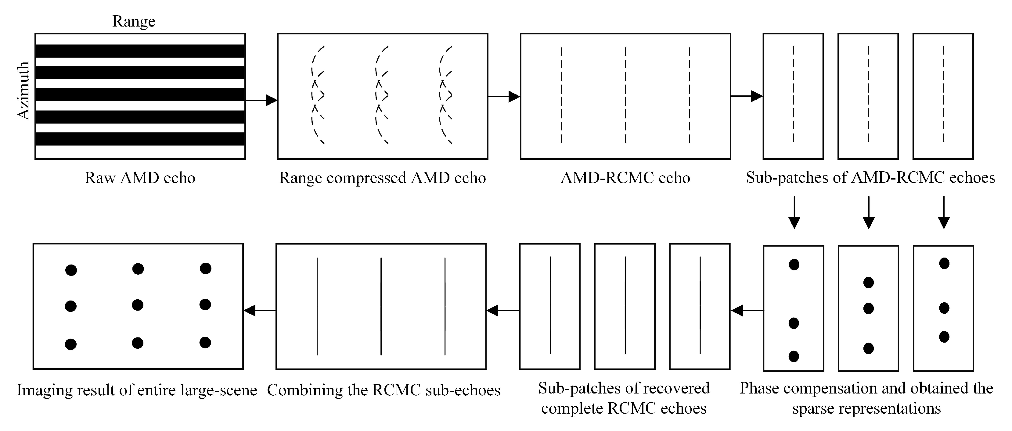
The detailed steps of the proposed SSR-AMDIA are demonstrated in Figure 2. First of all, the raw AMD echo is range compressed, and the range cells migration is corrected. Then, the entire AMD-RCMC echo is split into a series of AMD-RCMC sub-echoes along the range direction. Next, as the critical step, a set of PCFs are redesigned based on the RCMC sub-echoes. By multiplying each RCMC sub-echo with its corresponding PCF in the range-frequency domain, each complete PC-RCMC sub-echo can obtain a sparse representation in the Doppler domain. Subsequently, the accurate estimations of the complete PC-RCMC sub-echoes are recovered from the AMD-PC-RCMC sub-echoes using the CS method. In this article, we employ the Generalized Orthogonal Matching Pursuit (GOMP) algorithm [26] to reconstruct the full PC-RCMC sub-echoes in order to remove any potential error impacts of various CS techniques, as in the SOA-AMDIA [3,17,20,27]. Then, the accuracy estimations of the complete RCMC sub-echoes can be obtained by multiplying the complete PC-RCMC sub-echoes with the conjugation of the previously mentioned PCFs. Finally, by combining each reconstructed RCMC sub-echo, the reconstructed RCMC echo of the entire imaging scene can be acquired, and then after azimuth compression, a satisfied imaging result can be obtained.

Next, we describe the specific derivation steps of the proposed SSR-AMDIA in detail.

3.1. Range Compression and Range Cell Migration Correction

First, $s_m(t,\eta )$ should accomplish the range Fourier transform to obtain the range-frequency domain signal $S_m(f_r,\eta )$, which can be expressed as

$$\begin{array}{c}\hfill S_m(f_r,\eta )=w_r\left(f_r\right)w_a\left(\eta \right)exp\left(\frac{-j\pi f_r^2}{K_r}\right)exp\left\{\frac{-j4\pi (f_c+f_r)R_P\left(\eta \right)}{c}\right\}\end{array}$$

(9)

where $f_r$ denotes the range frequency.

Then, the range compressed signal $s_{m\mathrm{rc}}(t,\eta )$ can be obtained after range compression, and the range Doppler domain signal $S_{m\mathrm{rc}}(t,f_{\eta })$ can be presented as

$$\begin{array}{c}\hfill S_{m\mathrm{rc}}\left(t,f_{\eta }\right)=p_r\left(t-\frac{2R_{rd}\left(f_{\eta }\right)}{c}\right)w_a\left(f_{\eta }\right)exp\left(\frac{-j4\pi f_c{R}_{rd}\left(f_{\eta }\right)}{c}\right)\end{array}$$

(10)

where $p_r$ stands for the sinc function and $f_{\eta }$ is the azimuth frequency. The Doppler instantaneous distance $R_{rd}\left(f_{\eta }\right)$ can be written as

$$\begin{array}{c}\hfill R_{rd}\left(f_{\eta }\right)\approx R_0+\frac{v_a^2}{2R_0}{\left(\frac{f_{\eta }}{K_a}\right)}^2\end{array}$$

(11)

where $R_0$ is shortest distance between the platform and the target. $K_a$ is Doppler chirp rate. The second term of (11) is the range cells migration term.

After RCMC and the azimuth Inverse Fourier Transform (AIFT), the AMD-RCMC signal $s_{m\mathrm{rcmc}}(t,\eta )$ is demonstrated as

$$\begin{array}{c}\hfill s_{m\mathrm{rcmc}}(t,\eta )=p_r\left(t-\frac{2R_0}{c}\right)w_a\left(\eta \right)exp\left(\frac{-j4\pi f_c{R}_P\left(\eta \right)}{c}\right)\end{array}$$

(12)

3.2. Reconstructing the Sub-Echoes

To reduce the residual phase error of the range far-field targets, the AMD-RCMC echo is split into K sub-patches along the range direction. Since target range locations are determined after RCMC, the range segmentation will not distort the adjacent sub-scenes. To redesign the more effective PCFs, k-th AMD-RCMC sub-echo $s_{m\mathrm{rcmc}}^{k_{th}}(t,\eta )$ transforms to range-frequency domain, which is described as

$$\begin{array}{c}\hfill S_{m\mathrm{rcmc}}^{k_{th}}\left(f_r,\eta \right)=w_r\left(f_r\right)w_a\left(\eta \right)exp\left(\frac{-j4\pi f_r{R}_0}{c}\right)exp\left(\frac{-j4\pi f_c{R}_P\left(\eta \right)}{c}\right)\end{array}$$

(13)

Thus, k-th redesigned PCF ${\theta }_{\mathrm{ref}}^{k_{th}}\left(f_r,\eta \right)$ is defined as

$$\begin{array}{c}\hfill {\theta }_{\mathrm{ref}}^{k_{th}}\left(f_r,\eta \right)=exp\left(\frac{j4\pi f_r{R}_{\mathrm{ref}0}^{k_{th}}}{c}\right)exp\left(\frac{j4\pi f_c{R}_{\mathrm{ref}}^{k_{th}}\left(\eta \right)}{c}\right)\end{array}$$

(14)

where $R_{\mathrm{ref}0}^{k_{th}}$ is the shortest slant range of k-th reference point $P_{\mathrm{ref}}^{k_{th}}(x_{\mathrm{ref}}^{k_{th}},y_{\mathrm{ref}}^{k_{th}},0)$. The ${\mathit{R}}_{\mathrm{ref}}^{k_{th}}$ represents the slant range between $P_{\mathrm{ref}}^{k_{th}}(x_{\mathrm{ref}}^{k_{th}},y_{\mathrm{ref}}^{k_{th}},0)$ and the moving platform $(x_i,y_i,h)$. It can be expressed as

$$R_{\mathrm{ref}}^{k_{th}}\left(\eta \right)=\sqrt{{(x_i-x_{\mathrm{ref}}^{k_{th}})}^2+{\left(y_i-y_{\mathrm{ref}}^{k_{th}}\right)}^2+h^2}$$

(15)

Next, the azimuth missing redesigned PCF ${\mathit{\theta }}_{m\mathrm{ref}}^{k_{th}}$ is acquired based on (6), that is

$$\begin{array}{c}\hfill {\mathit{\theta }}_{m\mathrm{ref}}^{k_{th}}={\mathsf{\Lambda }}_m{\mathit{\theta }}_{\mathrm{ref}}^{k_{th}}\end{array}$$

(16)

The PCF designation is the key step of the proposed SSR-AMDIA. A sparse PC-RCMC sub-echo $S_{\mathrm{pc}}^{k_{th}}(t,f_{\eta })$ that is likewise the waiting-recovering signal may be generated in the Doppler domain by multiplying $S_{\mathrm{rcmc}}^{k_{th}}\left(f_r,\eta \right)$ by ${\theta }_{\mathrm{ref}}^{k_{th}}\left(f_r,\eta \right)$, which is represented by

$$\begin{array}{c}\hfill S_{\mathrm{pc}}^{k_{th}}(t,f_{\eta })={\mathrm{FFT}}_a\left[{\mathrm{IFFT}}_r\left[S_{\mathrm{rcmc}}^{k_{th}}(f_r,\eta ){\theta }_{\mathrm{ref}}^{k_{th}}\left(f_r,\eta \right)\right]\right]\end{array}$$

(17)

where ${\mathrm{FFT}}_a\left[·\right]$ and ${\mathrm{IFFT}}_r\left[·\right]$ are azimuth Fast Fourier Transform and range Inverse Fast Fourier Transform, respectively.

Since the main purpose of the proposed SSR-AMDIA is to reconstruct $S_{\mathrm{pc}}(t,f_{\eta })$, its sparsity is vital for the signal reconstruction.

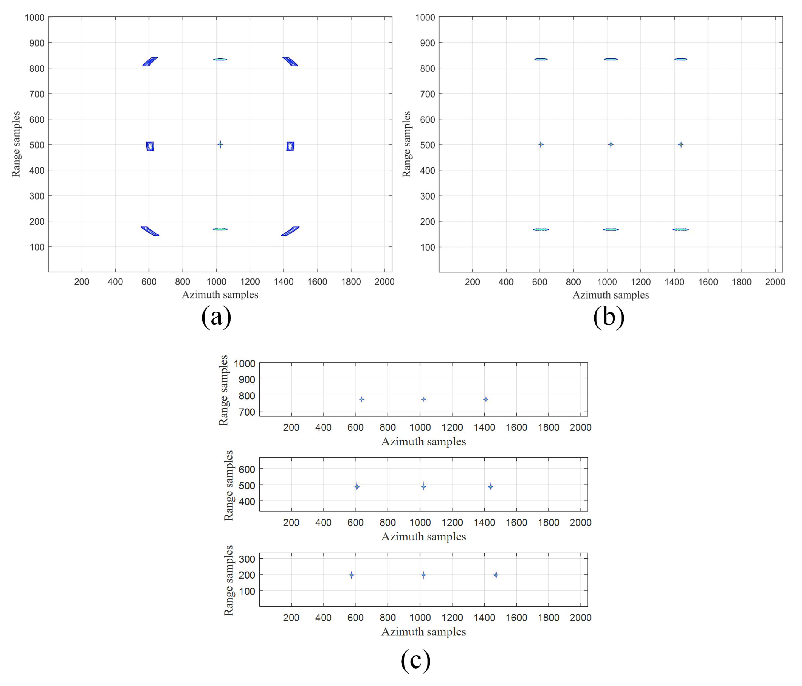
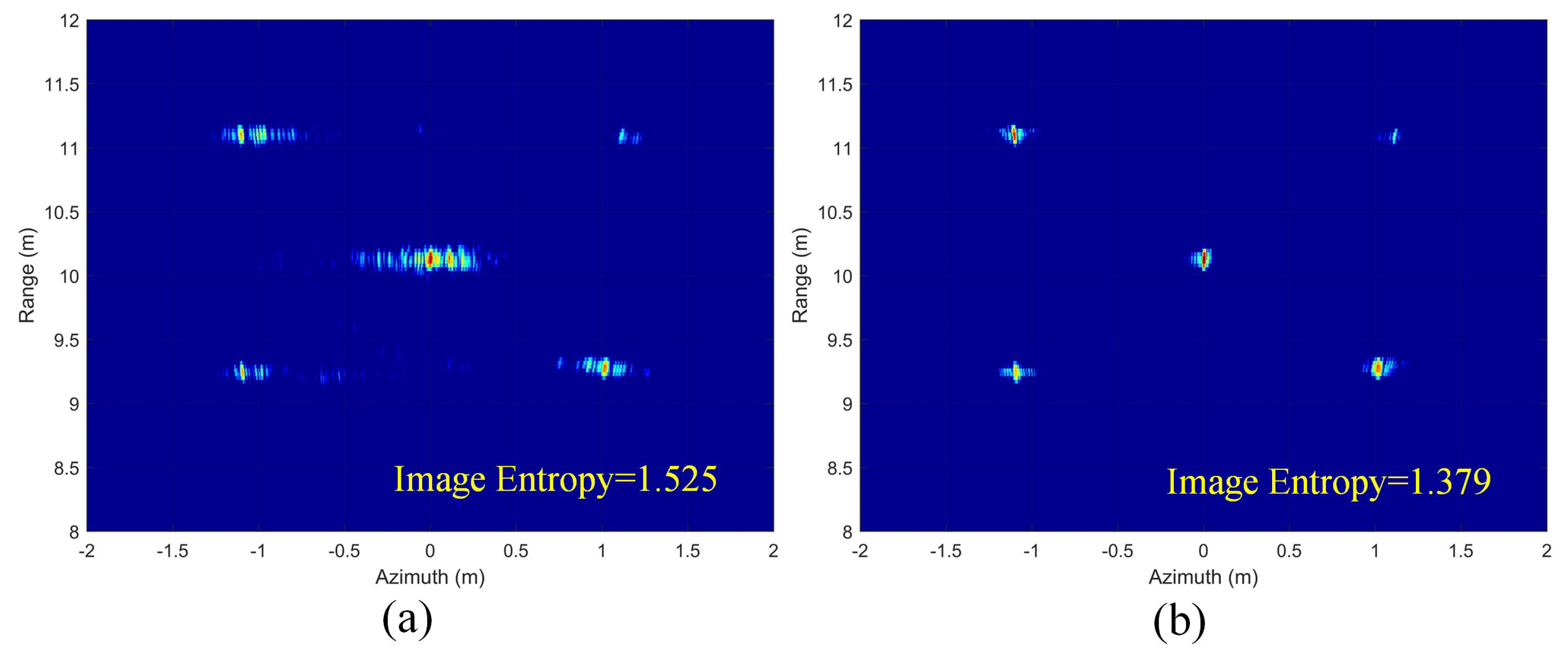
To evaluate the focusing performance of the redesigned PCFs, $S_{\mathrm{pc}}(t,f_{\eta })$ results obtained by different methods are shown in Figure 3. There are nine targets in the imaging scene, and the SOA-AMDIA’s $S_{\mathrm{pc}}(t,f_{\eta })$ is shown in Figure 3a. Obviously, only the center point is well-focused. The significant defocus can be easily found on the edge targets. Therefore, the effectiveness of SOA-AMDIA’s PCF for larger scenarios is limited. Moreover, Figure 3b is imaged using the proposed SSR-AMDIA before the sub-echo segmentation. Compared with the Figure 3a, the azimuth far-field targets at the center range are well-focused. However, it still cannot remove the residual phase error caused by the range differences. The range edge targets are still defocused. When a series of segmented ${\theta }_{\mathrm{ref}}^{k_{th}}\left(f_r,\eta \right)$ are used, the most sparse $S_{\mathrm{pc}}(t,f_{\eta })$ can be obtained by observing Figure 3c. The two-dimensional residual phase errors of the borderline targets are significantly reduced. The focusing performance of the redesigned PCFs is validated.

Next, the detailed reconstruction steps of the proposed SSR-AMDIA are introduced as follows. Firstly, the small size phase-compensated signal ${\mathit{s}}_{y\mathrm{pc}}^{k_{th}}$ can be demonstrated as the same as (7)

$$\begin{array}{c}\hfill {\mathit{s}}_{y\mathrm{pc}}^{k_{th}}={\tilde{\mathit{I}}}_y{\mathit{s}}_{m\mathrm{pc}}^{k_{th}}\end{array}$$

(18)

$s_{y\mathrm{pc}}^{k_{th}}(t,\eta )$ must be segmented into several one-dimensional range signals in order to accommodate the one-dimensional signal recovery processing. The q-th ($1\le q\le N_R$) range signal can be expressed as ${\mathit{s}}_{y\mathrm{pc}}^{k_{th}}(t_q,\eta )$, where $N_R$ denotes the number of entire range gates. In the proposed SSR-AMDIA, the q-th estimated range signal $S_{\mathrm{pc}}^{k_{th}}(t_q,f_{\eta })$ is regarded as the signal $\mathit{x}$ in CS method, while $S_{y\mathrm{pc}}^{k_{th}}(t_q,\eta )$ is considered as the compressed signal vector $\mathit{y}$. Accordingly, since $S_{\mathrm{pc}}^{k_{th}}(t_q,f_{\eta })$ is direct sparse, ${\mathsf{\Phi }}_{y\mathrm{AIFT}}$ is understood as being the sensing matrix $\mathit{A}$. First, the complete AIFT matrix ${\mathsf{\Phi }}_{\mathrm{AIFT}}$ is illustrated as

$$\begin{array}{cc}\hfill & {\mathsf{\Phi }}_{\mathrm{AIFT}}=\frac{1}{N_A}\left[\begin{array}{ccc}exp\left(j\frac{2\pi {\eta }_1{\eta }_1}{{\eta }_{N_A}}\right)& \cdots & exp\left(j\frac{2\pi {\eta }_1{\eta }_{N_A}}{{\eta }_{N_A}}\right)\\ ⋮& \ddots & ⋮\\ exp\left(j\frac{2\pi {\eta }_{N_A}{\eta }_1}{{\eta }_{N_A}}\right)& \cdots & exp\left(j\frac{2\pi {\eta }_{N_A}{\eta }_{N_A}}{{\eta }_{N_A}}\right)\end{array}\right]\hfill \end{array}$$

(19)

Similar to the Equation (6) and (16), the partial missing AIFT matrix ${\mathsf{\Phi }}_{m\mathrm{AIFT}}$ is obtained by

$$\begin{array}{c}\hfill {\mathsf{\Phi }}_{m\mathrm{AIFT}}={\mathsf{\Lambda }}_m{\mathsf{\Phi }}_{\mathrm{AIFT}}\end{array}$$

(20)

Similar to (7), the small size AIFT matrix ${\mathsf{\Phi }}_{y\mathrm{AIFT}}$ is gained by

$$\begin{array}{c}\hfill {\mathsf{\Phi }}_{y\mathrm{AIFT}}={\tilde{\mathit{I}}}_y{\mathsf{\Phi }}_{m\mathrm{AIFT}}\end{array}$$

(21)

Its size is equal to $(N_A-N_M)\times N_A$. Consequently, the sub-echoes reconstructing process can be formulated as

$$\begin{array}{c}\underset{S_{\mathrm{pc}}^{k_{th}}(t_q,f_{\eta })}{min}{\Vert S_{\mathrm{pc}}^{k_{th}}(t_q,f_{\eta })\Vert }_1,\\ \mathrm{s}.\mathrm{t}.{\Vert {\mathsf{\Phi }}_{y\mathrm{AIFT}}{S}_{\mathrm{pc}}^{k_{th}}(t_q,f_{\eta })-s_{y\mathrm{pc}}^{k_{th}}(t_q,\eta )\Vert }_2\le ϵ\end{array}$$

(22)

where $ϵ$ denotes the threshold value.

To eliminate the possible error effects of different recovery methods, the estimated ${\widehat{S}}_{\mathrm{pc}}^{k_{th}}(t_q,f_{\eta })$ is reconstructed using the GOMP algorithm in this article.

Table 1. The specific steps for the GOMP algorithm based on $s_{y\mathrm{pc}}^{k_{th}}(t_q,\eta )$.

Step 1	Input the indices number of each selection P, the maximum number of iterations $I_{max}$, the threshold parameter $ϵ$ and ${\mathsf{\Phi }}_{y\mathrm{AIFT}}$;
Step 2	Initialize the iteration parameter $It$ = 1, let the residue signal ${\mathit{r}}^0={\mathit{s}}_{y\mathrm{pc}}^{k_{th}}(t_q,\eta )$, and set a new sensing matrix ${\mathit{B}}^0=Ø$;
Step 3	Let $It=It+1$;
Step 4	Calculate the largest P values in $\left|〈{\mathit{r}}^{It-1},{\mathsf{\Phi }}_{y\mathrm{AIFT}}〉\right|$ from the largest to smallest and then the corresponding ${\mathit{\varphi }}_{{max}_p}$ are selected;
Step 5	Update matrix ${\mathit{B}}^{It}={\mathit{B}}^{It-1}\cup \left[{\mathit{\varphi }}_{{max}_1},\cdots ,{\mathit{\varphi }}_{{max}_P}\right]$ and calculate the estimated value of complete signal vector by $\widehat{\mathit{\alpha }}={\left({\left({\mathit{B}}^{It}\right)}^H{\mathit{B}}^{It}\right)}^{-1}{\left({\mathit{B}}^{It}\right)}^H{\mathit{s}}_{y\mathrm{pc}}^{k_{th}}(t_q,\eta )$, where H represents the conjugate transpose operation;
Step 6	Update residue signal ${\mathit{r}}^{It}={\mathit{s}}_{y\mathrm{pc}}^{k_{th}}(t_q,\eta )-{\mathit{B}}^{It}\widehat{\mathit{\alpha }}$;
Step 7	If $It=I_{max}$ or ${\Vert {\mathit{r}}^{It}\Vert }_2\le ϵ$, let ${\widehat{\mathit{S}}}_{\mathrm{pc}}^{k_{th}}(t_q,f_a)=\widehat{\mathit{\alpha }}$. Else go to Step 3.

or [26] contains the specific steps for the GOMP algorithm.

Once the reconstructed one-dimensional signals ${\widehat{S}}_{\mathrm{pc}}^{k_{th}}(t_q,f_{\eta })$ are combined, the k-th segment sub-echo ${\widehat{S}}_{\mathrm{pc}}^{k_{th}}(t,f_{\eta })$ can be acquired. It follows that the conjugation of ${\theta }_{\mathrm{ref}}^{k_{th}}\left(f_r,\eta \right)$ must be compensated in order to obtain the k-th segment ${\widehat{s}}_{\mathrm{rcmc}}^{k_{th}}(t,\eta )$, which is represented by

$$\begin{array}{c}\hfill {\widehat{S}}_{\mathrm{rcmc}}^{k_{th}}(f_r,\eta )={\widehat{S}}_{\mathrm{pc}}^{k_{th}}(f_r,\eta )conj\left({\theta }_{\mathrm{ref}}^{k_{th}}\left(f_r,\eta \right)\right)\end{array}$$

(23)

3.3. Combining the Sub-Echoes and Entire Scene Imaging

To obtain the reconstructed complete RCMC echo ${\widehat{\mathit{s}}}_{\mathrm{rcmc}}$ of entire imaging scene, a series of ${\widehat{\mathit{s}}}_{\mathrm{rcmc}}^{k_{th}}$ are combined in sequence, that is

$$\begin{array}{c}\hfill {\widehat{\mathit{s}}}_{\mathrm{rcmc}}=⌊{\widehat{\mathit{s}}}_{\mathrm{rcmc}}^{1_{st}},\cdots ,{\widehat{\mathit{s}}}_{\mathrm{rcmc}}^{k_{th}},\cdots ,{\widehat{\mathit{s}}}_{\mathrm{rcmc}}^{K_{th}}⌋\end{array}$$

(24)

where $⌊·⌋$ denotes the combination operation.

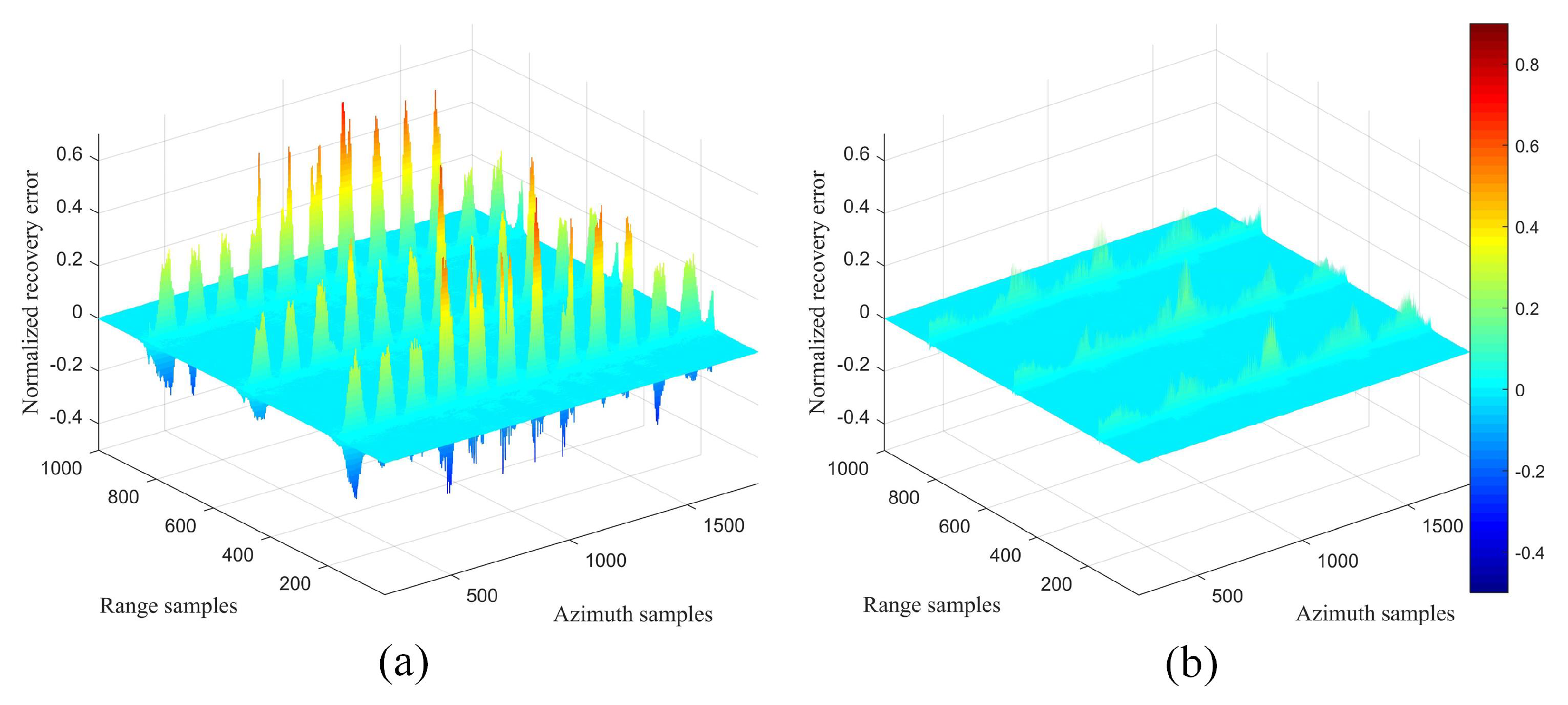
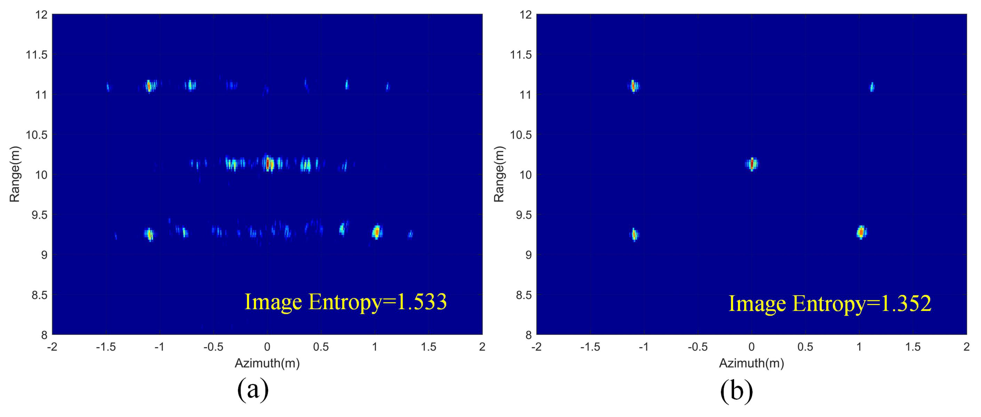
The normalized recovery error results between $s_{\mathrm{rcmc}}(t,\eta )$ and ${\widehat{s}}_{\mathrm{rcmc}}(t,\eta )$ are illustrated in Figure 4. Figure 4a is obtained using the SOA-AMDIA and Figure 4b is obtained using the proposed SSR-AMDIA. In order to quantitatively evaluate the reconstruction performance, the average normalized recovery error $E_a$ is defined as

$$\begin{array}{c}\hfill E_a=\mathrm{mean}\left(\sum _{}^{t\in Q_R}\sum _{\eta =0}^{N_A-1}\left(\left|\frac{s_{\mathrm{rcmc}}\left(t,\eta \right)}{max\left(s_{\mathrm{rcmc}}\left(t,\eta \right)\right)}\right|-\left|\frac{{\widehat{s}}_{\mathrm{rcmc}}\left(t,\eta \right)}{max\left({\widehat{s}}_{\mathrm{rcmc}}\left(t,\eta \right)\right)}\right|\right)\right)\end{array}$$

(25)

where $Q_R$ represents the range cells set corresponding to the presence of targets after RCMC, and $\mathrm{mean}\left(·\right)$ denotes the average function. According to Figure 4, $E_a$ of Figure 4a is equal to 0.087, which is almost half to that of Figure 4b, which is equal to 0.179. Therefore, the proposed SSR-AMDIA obviously has a better reconstruction performance.

Finally, since a satisfied complete RCMC echo of the entire scene is estimated, an excellent-focused image can be obtained via azimuth compression.

4. Parameter Analysis

As mentioned before, we consider extending the maximum DOFs of SOA-AMDIA in azimuth and range directions, respectively. Thus, the range segmentation is applied in the proposed SSR-AMDIA. However, the identical segmentation idea cannot be exploited to enlarge the azimuth imaging scope. Azimuth segmentation may result in too few azimuth samples available in some sub-apertures, especially in the case of random missing. Sub-apertures with a high AMR will be detrimental to complete sub-aperture reconstruction [3]. Hence, although the proposed SSR-AMDIA extends the azimuth maximum DOF, it has a limitation. Moreover, there is no limit to the maximum range imaging scope of the proposed SSR-AMDIA under a proper segmentation. We next analyze the azimuth maximum DOF and range segmentation strategy of the proposed algorithm. The computational complexity advantage is also investigated.

4.1. Azimuth Maximum Depth of Focus

In 2005, B. Rigling analyzed the imaging scene size limits for the PFA in the monostatic SAR system situation [28]. When the absolution value of residual Quadratic Phase Error after the PFA (PFA-QPE) $\left|{\mathsf{\Phi }}_{\mathrm{QPE}}\right|<\pi /4$, the PFA’s maximum well-focused radius $r_{max}$ can be expressed as

$$\begin{array}{c}\hfill r_{max}<{\rho }_a\sqrt{\frac{2R_{\mathrm{ref}0}}{\lambda }}\end{array}$$

(26)

where ${\rho }_a$ and $\lambda$ denote the azimuth resolution and wavelength, respectively. The prerequisite for applying (26) is that there are no unknown motion measurement errors during the flight. Otherwise, the phase errors will lead to an irreparable defocus to the image long before the far-field approximation (26) breaks down.

In 2016, L. Gorham and B. Riging further derived the imaging scene size limits for the PFA in the linear flight case [18]. The residual PFA-QPE ${\mathsf{\Phi }}_{\mathrm{QPE}}$ can be written as

$$\begin{array}{c}\hfill {\mathsf{\Phi }}_{\mathrm{QPE}}=-\frac{L_a^2\pi }{2\lambda }\left(\frac{1}{R_{P0}}-\frac{2}{R_{\mathrm{ref}0}}-\frac{y^2}{R_{P0}^3}+\frac{R_{P0}}{R_{\mathrm{ref}0}^2}\right)\end{array}$$

(27)

where $L_a$ is the length of synthetic aperture and $R_{P0}$ can be calculated as

$$\begin{array}{c}\hfill R_{P0}={\left.R_P\right|}_{y_i=0}=\sqrt{{\left(x_i-x\right)}^2+{\left(0-y\right)}^2+h^2}\end{array}$$

(28)

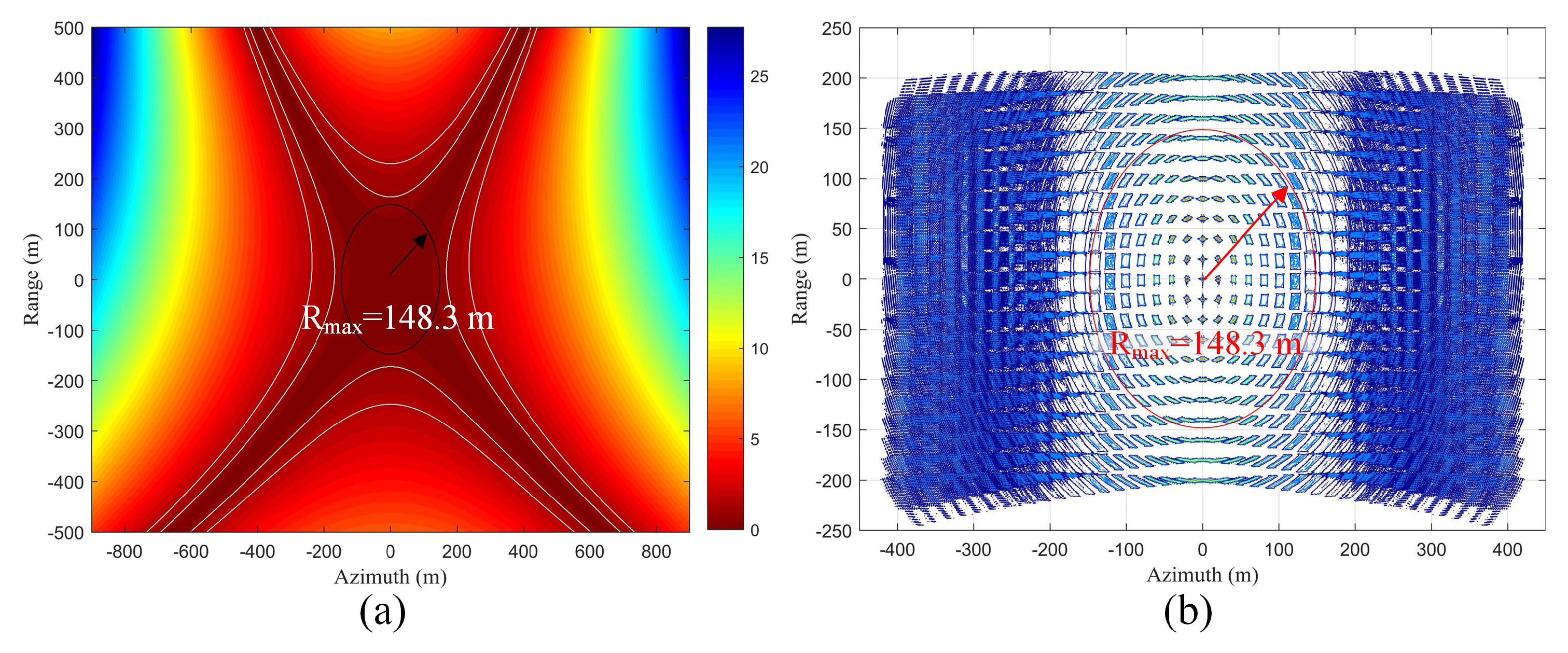
The value of ${\mathsf{\Phi }}_{\mathrm{QPE}}$ is related to the position of targets. Assume $f_c=1$ GHz, $R_{\mathrm{ref}0}=3300$ m, ${\mathsf{\Phi }}_{\mathrm{QPE}}$ result in different positions is shown in Figure 5a. The maximum focus area is limited to a circle of which radius equals 148.3 m after the PFA imaging. However, since the SOA-AMDIA only utilizes the phase compensation process of PFA, the maximum DOF of ${\mathit{S}}_{\mathrm{pc}}(t,f_{\eta })$ decreases rapidly [29,30].

To illustrate this phenomenon more clearly, we form $S_{\mathrm{pc}}(t,f_{\eta })$ using the SOA-AMDIA with a regular grid in actual coordinates in Figure 5b. Due to the impact of the range cells migration and the residual phase error, the azimuth edge targets of Figure 5b are distorted and defocused severely while only the centroid is excellent-focused. Although it is clearly sparser than the dense time domain signal, the maximum DOF of $S_{\mathrm{pc}}(t,f_{\eta })$ is only 25 m, much less than 148.3 m. The aforementioned conclusion has been verified in simulation. The low-quality $S_{\mathrm{pc}}(t,f_{\eta })$ will impair full echo reconstruction. The applicable imaging scope of the SOA-AMDIA will be significantly reduced.

In response to this problem, the range cells migration effect of the raw echo is removed by the proposed SSR-AMDIA. Then, a new PCF is redesigned to enhance the sparsity of $S_{\mathrm{pc}}(t,f_{\eta })$ and to extend the maximum azimuth DOF.

First, the residual phase error ${\mathsf{\Phi }}_{\mathrm{E}}$ between the scattering point and the reference point can be represented as

$$\begin{array}{c}\hfill {\mathsf{\Phi }}_{\mathrm{E}}=-\frac{4\pi \Delta R\left(\eta \right)}{\lambda }\end{array}$$

(29)

where $\Delta R=R_P-R_{\mathrm{ref}}$ is the differential slant range, and the expressions of $R_P$ and $R_{\mathrm{ref}}$ can be found in (3) and (15), respectively. The second-order Taylor series approximation of $\Delta R$ is performed as

$$\begin{array}{cc}\hfill \Delta R\left(\eta \right)& \approx {\left.\Delta R\right|}_{\eta =0}+{\left.\frac{\partial \Delta R}{\partial \eta }\right|}_{\eta =0}\eta +{\left.\frac{{\partial }^2\Delta R}{{\partial }^2\eta }\right|}_{\eta =0}\frac{{\eta }^2}{2}\hfill \\ \hfill & \approx \left(R_{P0}-R_{\mathrm{ref}0}\right)+\left({\left.\frac{\partial R_P}{\partial \eta }\right|}_{\eta =0}-{\left.\frac{\partial R_{\mathrm{ref}}}{\partial \eta }\right|}_{\eta =0}\right)\eta +\left({\left.\frac{{\partial }^2{R}_P}{\partial {\eta }^2}\right|}_{\eta =0}-{\left.\frac{{\partial }^2{R}_{\mathrm{ref}}}{\partial {\eta }^2}\right|}_{\eta =0}\right)\frac{{\eta }^2}{2}\hfill \end{array}$$

(30)

Let the monostatic SAR system moves at a constant speed in the azimuth direction ($+y$ direction), the first and second derivatives of $R_P$ and $R_{\mathrm{ref}}$ can be calculated as

$$\left\{\begin{array}{c}\frac{\partial R_P}{\partial \eta }=-\frac{\left(y-y_i\right)}{R_P}\frac{\partial y_i}{\partial \eta }\hfill \\ \frac{\partial R_{\mathrm{ref}}}{\partial \eta }=\frac{y_i}{R_{\mathrm{ref}}}\frac{\partial y_i}{\partial \eta }\hfill \\ \frac{{\partial }^2{R}_P}{\partial {\eta }^2}=-\frac{1}{R_P}\left(\left(y-y_i\right)\frac{{\partial }^2{y}_i}{\partial {\eta }^2}\left.-{\left(\frac{\partial y_i}{\partial \eta }\right)}^2+{\left(\frac{\partial R_P}{\partial \eta }\right)}^2\right)\right.\hfill \\ \frac{{\partial }^2{R}_{\mathrm{ref}}}{\partial {\eta }^2}=\frac{1}{R_{\mathrm{ref}}}\left(y_i\frac{{\partial }^2{y}_i}{\partial {\eta }^2}+{\left(\frac{\partial y_i}{\partial \eta }\right)}^2\right.\left.-{\left(\frac{\partial R_{\mathrm{ref}}}{\partial \eta }\right)}^2\right)\hfill \end{array}\right.$$

(31)

where $\partial y_i/\partial \eta =L_a/2$ and ${\partial }^2{y}_i/\partial {\eta }^2=0$.

The residual QPE after RCMC and phase compensation (PC-RCMC-QPE) ${\tilde{\mathsf{\Phi }}}_{\mathrm{QPE}}$ is thus computed as

$$\begin{array}{cc}\hfill {\tilde{\mathsf{\Phi }}}_{\mathrm{QPE}}& =-\frac{2\pi }{\lambda }\left({\left.\frac{{\partial }^2{R}_P}{\partial {\eta }^2}\right|}_{\eta =0}-{\left.\frac{{\partial }^2{R}_{\mathrm{ref}}}{\partial {\eta }^2}\right|}_{\eta =0}\right)\hfill \\ \hfill & =\frac{L_a^2\pi \left(y^2{R}_{\mathrm{ref}0}+R_{P0}^3-R_{P0}^2{R}_{\mathrm{ref}0}\right)}{2\lambda R_{P0}^3{R}_{\mathrm{ref}0}}\hfill \end{array}.$$

(32)

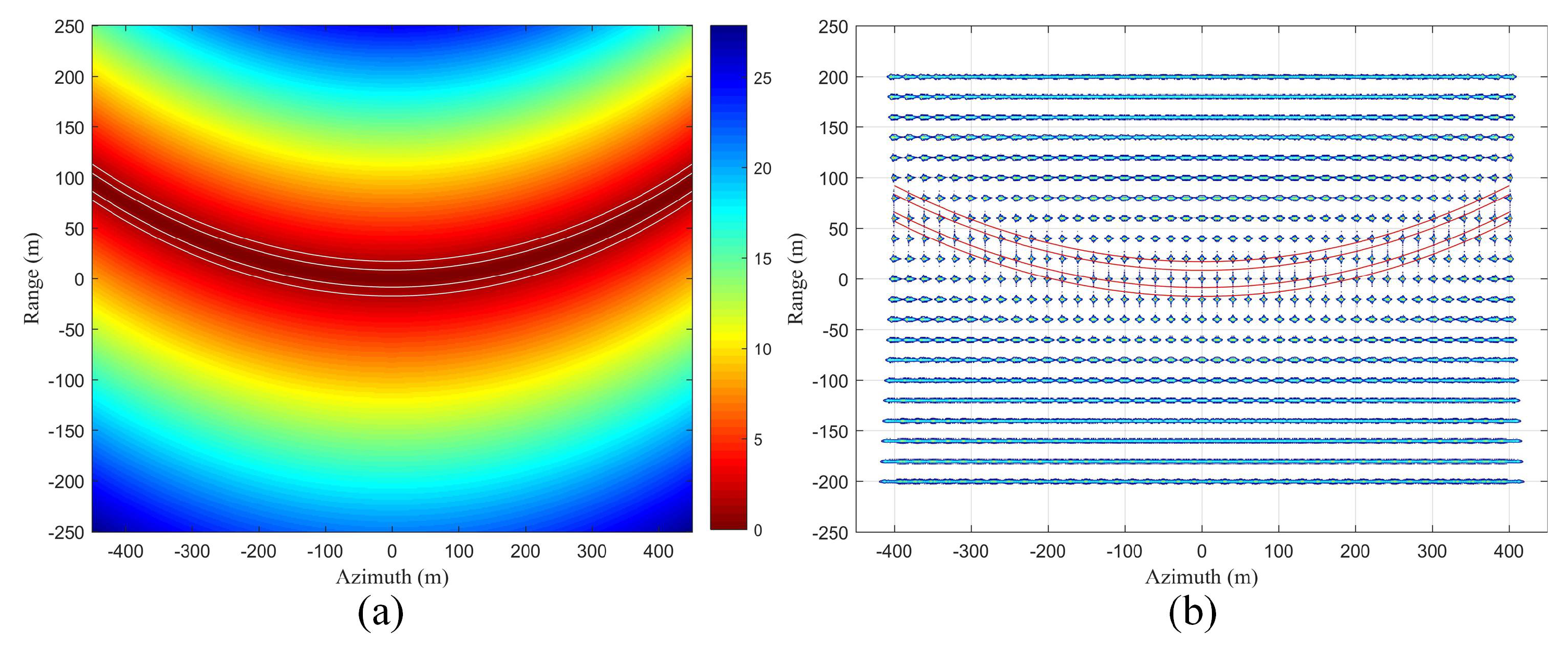
Suppose $f_c=1$ GHz, $R_{\mathrm{ref}0}=3300$ m, PC-RCMC-QPE ${\tilde{\mathsf{\Phi }}}_{\mathrm{QPE}}$ result in different positions is shown in Figure 6a and we form the calculated $S_{\mathrm{pc}}(t,f_{\eta })$ by (17) when $K=1$ with a regular grid in actual coordinates in Figure 6b.

Figure 6b is significantly sparser than Figure 5b. The azimuth maximum DOF is substantially enlarged. Let $\left|{\tilde{\mathsf{\Phi }}}_{\mathrm{QPE}}\right|=\pi /2$ and $x=0$, the azimuth coordinate $y_{\mathrm{QPE}}$ can be calculated as

$$\begin{array}{c}\hfill y_{\mathrm{QPE}}=\pm \sqrt{{\left(\frac{L_a^2{R}_{\mathrm{ref}0}^3}{L_a^2+\lambda R_{\mathrm{ref}0}}\right)}^{2/3}-R_{\mathrm{ref}0}}\end{array}$$

(33)

Substitute the above-mentioned simulation parameters into (33), then two farthest points, $P_{y_1}(0,-194.05,0)$ and $P_{y_2}(0,194.05,0)$, that can achieve an excellent focus are obtained. Thus, the azimuth maximum DOF $\Delta y_{\mathrm{QPE}}=194.05-(-194.05)=388.10$ m, which is much larger than that in Figure 5b.

A strong sparsity of $S_{\mathrm{pc}}(t,f_{\eta })$ will facilitate the signal reconstruction. Hence, the azimuth maximum DOF of $S_{\mathrm{pc}}(t,f_{\eta })$ given by (33) is conservative compared to that of the final image. We found that $P_y(0,\pm 400,0)$ in the final image can still be accurately focused using the proposed algorithm with the above-mentioned simulation parameters. Conversely, the azimuth maximum DOF using SOA-AMDIA only reaches about $\pm 70$ m under identical simulation conditions.

4.2. Range Segmentation Strategy

Figure 6b exhibits the limited range maximum DOF of $S_{\mathrm{pc}}(t,f_{\eta })$ as well. Motivated by [15,19], the range segmentation is applied to expand the imaging scene scope in range direction. By observing Equation (32), the contour shape of ${\tilde{\mathsf{\Phi }}}_{\mathrm{QPE}}=0$ is a circle in the plane of $y=0$, of which radius equals $R_{\mathrm{ref}0}$. Since the imaging scene is limited in the plane of $z=0$, ${\tilde{\mathsf{\Phi }}}_{\mathrm{QPE}}=0$ can only be obtained at two points $(0,0,0)$ and $(2R_{\mathrm{ref}0},0,0)$. Similarly, the contour shapes of ${\tilde{\mathsf{\Phi }}}_{\mathrm{QPE}}=-\pi /2$ and ${\tilde{\mathsf{\Phi }}}_{\mathrm{QPE}}=\pi /2$ are two circles in the plane of $y=0$ with different radius. It indicates that only four targets can ensure $\left|{\tilde{\mathsf{\Phi }}}_{\mathrm{QPE}}\right|=\pi /2$ in the $y=z=0$ case.

Let $\left|{\tilde{\mathsf{\Phi }}}_{\mathrm{QPE}}\right|=\pi /2$ and $y=0$, the range coordinate $x_{\mathrm{QPE}}$ can be calculated as

$$\left\{\begin{array}{c}{x}_{\mathrm{QPE}}=x_i\pm \sqrt{{\left(\frac{L_a^2{R}_{\mathrm{ref}0}}{L_a^2-\lambda R_{\mathrm{ref}0}}\right)}^2-h^2},{\tilde{\mathsf{\Phi }}}_{\mathrm{QPE}}=-\frac{\pi }{2}\hfill \\ x_{\mathrm{QPE}}=x_i\pm \sqrt{{\left(\frac{L_a^2{R}_{\mathrm{ref}0}}{L_a^2+\lambda R_{\mathrm{ref}0}}\right)}^2-h^2},{\tilde{\mathsf{\Phi }}}_{\mathrm{QPE}}=\frac{\pi }{2}\hfill \end{array}\right.$$

(34)

Hence, $P_{x_1}(-17.3,0,0)$, $P_{x_2}(17.1,0,0)$, $P_{x_3}(6582.9,0,0)$ and $P_{x_4}(6617.3,0,0)$ are obtained by substituting the above-applied simulation parameters into (34). Obviously, only $P_{x_1}(-17.3,0,0)$ and $P_{x_2}(17.1,0,0)$ are located in the imaging scene. The range maximum DOF is $\Delta x_{\mathrm{QPE}}=17.1-(-17.3)=34.4$ m.

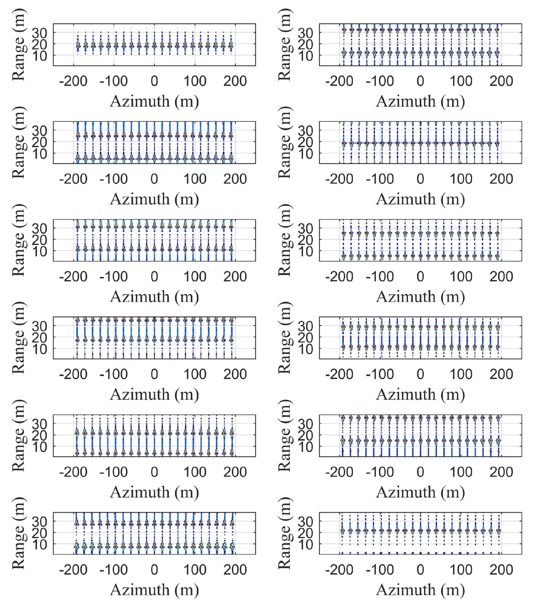
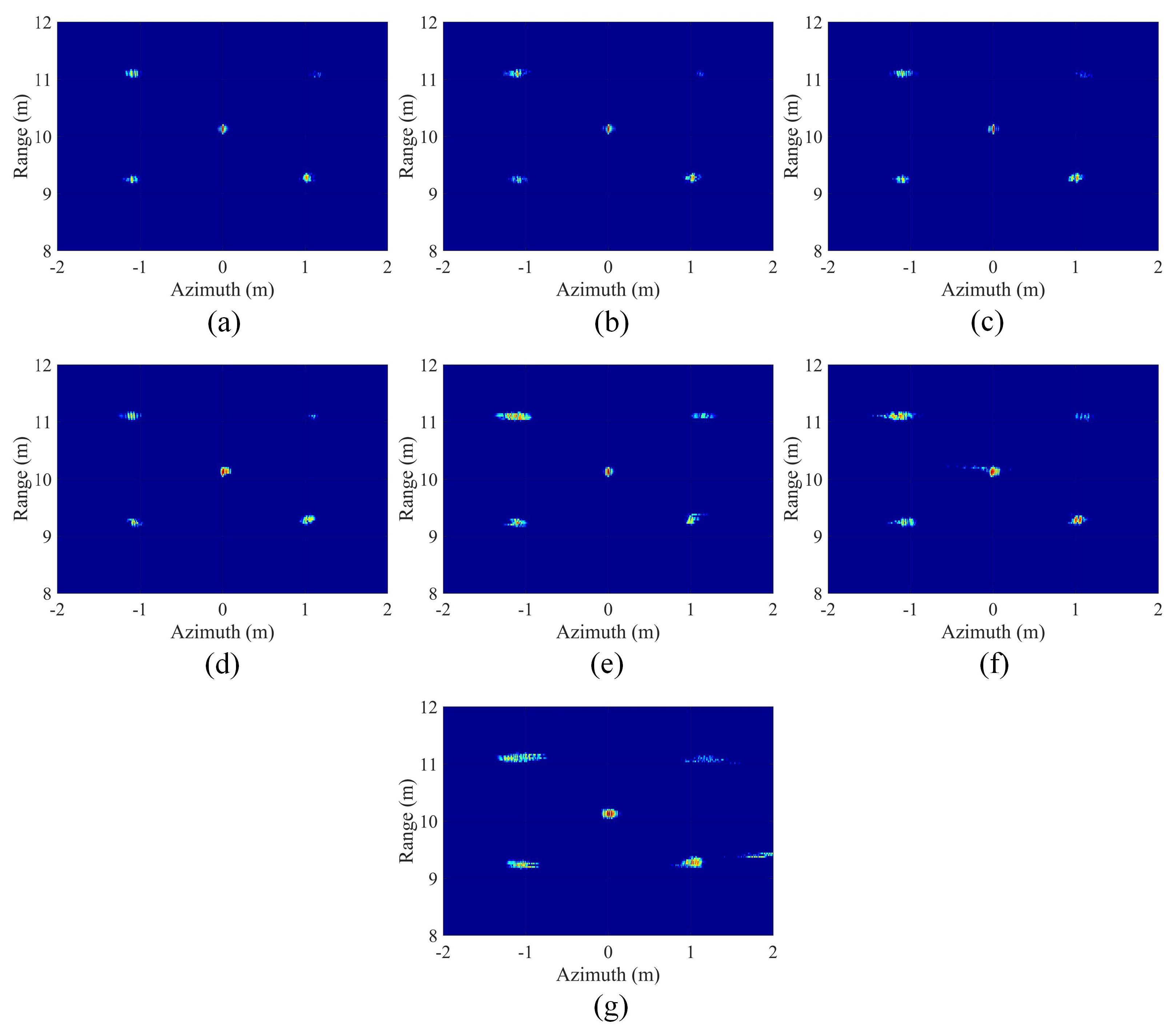
Obviously, when there is no target existing in the q-th range profile, the value of $S_{m\mathrm{pc}}(t_q,f_{\eta })$ is equal to zero. The zero row vectors do not need to be reconstructed. We assume that the number of the range profiles that exist targets equals $N_E$. Therefore, the $N_E$ range profiles of AMD-RCMC echo should be split into K sub-patches. The size of each sub-echo equals $(N_A-N_M)\times N_E/K$, where $N_E/K\le {\Delta x}_{\mathrm{QPE}}/\Delta x$ and $\Delta x$ denotes the interval of adjacent range cells.

Figure 7 demonstrates the simulated images of $S_{\mathrm{pc}}^{k_{th}}(t,f_{\eta })$ based on the aforementioned range segmentation strategy. By adequately segmenting the imaging scene within the azimuth maximum DOF, all targets corresponding to $S_{\mathrm{pc}}^{k_{th}}(t,f_{\eta })$ can be well-focused. The proposed SSR-AMDIA can guarantee the estimation accuracy of the complete echo in a larger imaging scene.

Moreover, since the proposed algorithm performs RCMC on the raw data before the range segmentation, the range position information of the sparse target is determined. Thus, it will not deteriorate the reconstruction error.

4.3. Computational Complexity

Assume that the number of entire range gates equals $N_R$ and $N_E$ sparse targets spread out along the range direction ($N_E\le N_R$). Since the range position information of the target is hidden in all range profiles before range compression and RCMC, no matter how many sparse targets exist, $N_R$ times reconstructions are required using the SOA-AMDIA. Contrarily, the proposed SSR-AMDIA only needs $N_E$ times reconstructions to complete echo reconstruction. Suppose the computational complexity of one-dimensional GOMP algorithm equals $\mathcal{O}$, then the computational complexity of the SOA-AMDIA is $N_R\mathcal{O}$, while that of the proposed SSR-AMDIA is equal to $N_E\mathcal{O}$. It implies that the computational complexity of the proposed SSR-AMDIA is $N_E/N_R$ times to that of SOA-AMDIA. Obviously, when fewer range profiles exist sparse targets, the computational complexity advantage of the proposed SSR-AMDIA is prominent.

5. Simulation and Real-Measured Experiment Validation

5.1. Simulation Verification of the Proposed SSR-AMDIA

An AMD-SAR imaging simulation is performed to evaluate the validation of the proposed SSR-AMDIA. Simulation parameters are shown in

Table 2. Key parameters for simulation.

Parameters	Value
Central frequency/$f_c$	1 GHz
Shortest central slant range / $R_{\mathrm{ref}0}$	3300 m
Signal frequency bandwidth / B	100 MHz
Range sampling rate / $f_s$	200 MHz
Pulse repetition frequency / PRF	197 Hz
Range samples / $N_R$	1002
Azimuth samples / $N_A$	2048
Azimuth missing ratio / AMR	50%

.

After allowing for 64 azimuth missing samples, we estimate that there are 64 available samples, making the AMR equals 50%. 600 range cells are segmented and reconstructed. Let the segment number $K=12$. Thus the range cell number of each sub-patch equals 50.

Figure 8a depicts a grid of point targets spaced at 20 m intervals extending from $-200$ m to $+200$ m in both range and azimuth directions. The scenario geometry is chosen to accentuate the defocus effects. The imaging result obtained using the SOA-AMDIA is demonstrated in Figure 8b. In Figure 8b, only the targets near the center point can be excellent-focused, while the peripheral targets are defocused. Contrarily, all targets can be clearly imaged by using the proposed SSR-AMDIA in the AMD echo situation, as shown in Figure 8c.

To exhibit the imaging performance of the proposed SSR-AMDIA in more detail, two far-field targets $P_A(200,200,0)$ and $P_B(-200,-200,0)$ are selected and marked with yellow squares in Figure 8b,c. These squares are zoomed for clearer exhibit in Figure 8d–g. In comparison to the Figure 8d,f, the false targets are eliminated using the proposed SSR-AMDIA, as shown in Figure 8e,g. While the azimuth resolution is maintained around 1 m, the azimuth Peak Side-lobe Ratio (PSLR) of $P_A^{\prime }$ and $P_B^{\prime }$ can reach $-10$ dB, which are much superior to that of $P_A$ and $P_B$. It can be observed that the PSLR results of $P_A^{\prime }$ and $P_B^{\prime }$ are not as good as the ideal PSLR result. This is because the proposed SSR-AMDIA is an aperture estimation algorithm. Therefore, there are inevitably estimation errors in the estimated aperture signal, resulting in imperfect focus in the final imaging result. However, compared to SOA-AMDIA, its focusing performance has been significantly improved. Thus, the effectiveness of the proposed SSR-AMDIA is verified. The limits of the imaging scene size have been significantly expanded. The imaging quality of far-field targets has been improved. Moreover, the running times of the SOA-AMDIA and proposed SSR-AMDIA are calculated by the average of 50 times Monte Carlo simulations. The simulations are manipulated with the laptop that was configured with the Intel Core i5-1135G7 CPU, eight cores, and 16-GB RAM. The running time of the SOA-AMDIA equals 459.52 s while that of the proposed SSR-AMDIA equals 238.33 s, almost half of the former result. Therefore, the computational complexity advantage of the proposed SSR-AMDIA has been verified.

5.2. Measured Data Verification of the Proposed SSR-AMDIA

In order to further explore the theoretical analyses offered in this study, a real measured SAR experiment is designed and implemented based on a 77GHz millimeter-wave radar. As shown in Figure 9a, the radar is placed on an electric track 1.40 m above the ground and moved in the azimuth direction at a speed of 2.13 cm/s, forming a linear aperture with a length of 1.57 m. When the millimeter-wave radar stops, the SAR system collects a two-dimensional SAR echo with a size of $1024\times 1960$.

First, to determine the azimuth and range maximum DOF, ${\tilde{\mathsf{\Phi }}}_{\mathrm{QPE}}$ is analyzed based on the measured SAR parameters. Substitute the related experiment parameters into (33) and (34), the two-dimensional maximum DOF can achieve 2.04 m and 0.32 m, respectively. We place five triangle reflectors in the scene based on the theoretical analysis. Target1 (11.10, −1.10), Target2 (11.10, 1.12), Target4 (9.24, −1.10), and Target5 (9.28, 1.02) are placed on the a square’s four vertices. Additionally, Target3 (10.12, 0.00) is placed in the center, as shown in Figure 9b. Figure 9c displays the image result obtained using the Range Doppler algorithm with the real measured complete echo.

The AMD echo in the first experiment is produced by a periodic gap that occurs every 40 pulses. Hence, the AMR is equal to 50%. Figure 10a,b illustrate the final images focused by using SOA-AMDIA and the proposed SSR-AMDIA, respectively. Obviously, the SOA-AMDIA cannot effectively reconstruct a satisfied image. On the other hand, all five point targets are accurately focused through the proposed SSR-AMDIA, as shown in Figure 10b. It implies that SSR-AMDIA can significantly improve the imaging performance in a larger imaging scope. Therefore, the effectiveness of the proposed algorithm is successfully verified in the real SAR data. Image Entropy (IE) is also presented to assess the imaging performance of the above-mentioned two imaging algorithms. The lower the IE, the superior the focus of the imaging algorithm. The IE values corresponding to Figure 10a,b are 1.533 and 1.352, respectively. Compared with Figure 9c, the imaging result obtained using the proposed SSR-AMDIA is almost identical. Additionally, the IE result of Figure 10b reaches the equivalent level of Figure 9c. Thus, the proposed algorithm obviously obtains a superior focusing performance.

Additionally, to comprehensively investigate the applicability of the proposed algorithm, a random AMD echo is set in the second experiment. Suppose that the SAR system is randomly subjected to 10 strong interferences during the data acquisition, and each interference causes 5% aperture data loss. In this case, AMR still equals 50% and the data size of random AMD echo is still $1024\times 980$. Figure 11 demonstrates the imaging results comparison, which leads to the identical conclusion to that of Figure 10. The proposed algorithm can still accurately focus all targets while all targets obtained using the SOA-AMDIA are defocused. Compared with the IE $=1.525$ obtained in Figure 11a, the IE can achieve 1.379 using the proposed SSR-AMDIA. Therefore, its effectiveness is fully verified on the measured SAR data once more.

Moreover, the running times of the SOA-AMDIA and proposed SSR-AMDIA are calculated by the average of 50 times Monte Carlo simulations.

Table 3. Running times of two AMD-SAR imaging algorithms under the real measured SAR data condition.

	SOA-AMDIA	SSR-AMDIA
50% Periodic Missing	53.25	7.92
50% Random Missing	29.39	7.04

shows the running time results. It can be found that the running time of the proposed SSR-AMDIA is much smaller than that of the SOA-AMDIA under both 50% periodic missing and 50% random missing conditions. Specifically, the proposed SSR-AMDIA needs 7.92 s to reconstruct the complete echo under periodic conditions, which is only about 1/7 of the existing method. Furthermore, in the random case, the running time of the proposed algorithm can be about 4 times faster than the SOA-AMDIA. A superior imaging result may be acquired more efficiently with the proposed SSR-AMDIA.

5.3. Imaging Performance Effects on Different Azimuth Missing Ratios

Moreover, in order to evaluate the imaging performance effects of the proposed SSR-AMDIA on different AMRs, a series of simulations based on real measured SAR data are designed and implemented. We assume that the radar system will be subjected to 11–17 strong interferences during the motion, and each substantial interference will result in 5% azimuth data loss. Therefore, the AMR will gradually increase from 55% to 85%. The imaging results obtained by the proposed SSR-AMDIA are shown in Figure 12.

Obviously, when AMR $\le 70\%$, the proposed SSR-AMDIA can obtain satisfactory imaging results. Targets in the imaging scene are well-focused. When AMR $>70\%$, the imaging quality of SSR-AMDIA gradually decreases, and the imaging results have obvious side-lobes along the azimuth direction. This situation will further deteriorate as AMR rises. In order to measure the imaging quality of the proposed method in different AMR cases, we also introduce IE to quantitatively analyze the imaging results, as Figure 13a shows.

In all AMR cases, the image focusing performance of the proposed SSR-AMDIA is superior to that of the SOA-AMDIA. It can be found that the IE has a significant increase, reaching 1.424, when AMR $=75\%$. It is identical to the conclusion in Figure 12, indicating that when AMR $>70\%$, the imaging performance of the proposed SSR-AMDIA decreases obviously.

Additionally, we calculated and analyzed the running time of the two algorithms under different AMR conditions through 50 Monte Carlo experiments. The results are shown in Figure 13b. Same as the previous simulation and experimental results, the running time of SSR-AMDIA is much smaller than SOA-AMDIA. Concretely, the SSR-AMDIA takes only a few seconds to reconstruct the complete signal, which is an order of magnitude less than the SOA-AMDIA. So far, the imaging performance effects on different AMRs have been comprehensively analyzed. The proposed AMD-SAR imaging algorithm has obvious advantages.

6. Conclusions

In this paper, we propose SSR-AMDIA to solve the AMD-SAR imaging problem. The effectiveness of the proposed algorithm has been verified in both simulations and the measured SAR experiments. Additionally, we derive the two-dimensional maximum DOFs of the proposed algorithm and perform a rigorous theoretical analysis of the SSR-AMDIA’s imaging scope. Compared with SOA-AMDIA, the proposed method can eliminate the limitation of the range maximum focusable scope, while the azimuth maximum focusable scope can be expanded by about 6 times. Our work found that the SOA-AMDIA has unacceptable focusable imaging size in the case of small shortest instantaneous distance or synthetic aperture length. The algorithm proposed in this paper can cope with this problem well and improve the applicability of AMD-SAR imaging. Furthermore, the imaging performance effects on different AMRs have been investigated. When AMR $\le 70\%$, the proposed SSR-AMDIA can obtain satisfactory imaging results. It indicates that the proposed algorithm can handle most AMR cases. Furthermore, with the multi-dimensional development of radar signals, our next logical step is to deal with the AMD-SAR imaging problems under various robust waveforms [31,32].