Article

A Numerical Assessment and Prediction for Meeting the Demand for Agricultural Water and Sustainable Development in Irrigation Area

1
School of Architecture and Civil Engineering, Xi’an University of Science and Technology, Xi’an 710054, China
2
School of Water and Environment, Chang’an University, Xi’an 710054, China
3
Key Laboratory of Subsurface Hydrology and Ecological Effects in Arid Region of the Ministry of Education, Chang’an University, Xi’an 710054, China
4
Northwest Engineering Corporation Limited, Xi’an 710054, China
5
Department of Civil and Environmental Engineering, Technion, Haifa 32000, Israel
*
Author to whom correspondence should be addressed.
Remote Sens. 2023, 15(3), 571; https://doi.org/10.3390/rs15030571
Submission received: 13 December 2022 / Revised: 10 January 2023 / Accepted: 11 January 2023 / Published: 18 January 2023
(This article belongs to the Special Issue Remote Sensing in Natural Resource and Water Environment)

Abstract

:
The demand for agricultural water is a growing problem in irrigated regions across the globe, particularly in arid and semi-arid regions. Changes in the level of groundwater in irrigation districts will affect the flow of surface water connected to the aquifer, which may damage the sustainability of water resources and ecosystems. In this study, a two-dimensional unsteady flow model based on MODFLOW was constructed and three scenarios were established to assess the demand for agricultural water in the Jiaokou Irrigation District. The results show that the groundwater in the study area is basically balanced. However, the supply of irrigation water for summer irrigation is insufficient. The results of the model prediction indicate that when groundwater is primarily used for irrigation (scenario 1), the maximum water level decrease is 25 m, which is beyond this limit (15 m). When the ratio of groundwater to surface water is 2:1 for irrigation (scenario 2), the largest decrease in water level is approximately 10 m. Scenario 3 is proposed based on the Hanjiang-to-Weihe River Valley Water Diversion Project to prevent the salinization of soil owing to the rise in water level, and its result shows that the maximum decrease and buried depth are approximately 5 m and above 3 m, respectively, indicating that the scenario is more reasonable and sustainable. These findings provide theoretical guidance to protect water resources and prevent water pollution and should serve as a reference for rationally allocating water resources in other irrigation districts in arid and semi-arid areas.

1. Introduction

Water, energy, food, and ecology play significant roles in poverty reduction, human well-being, and regional sustainable development [1]. As an important guarantee of food security and ecological construction, water resource plays an important role in agricultural irrigation, urban development, and harmonious coexistence between human and nature [2,3,4]. As an important part of water resources, groundwater has become a major resource for irrigated agriculture, particularly in arid and semi-arid regions that cover approximately one-third of the Earth’s total land area and where water resources are scarce [5,6,7,8]. It has been reported that agriculture is one of the largest consumers of groundwater and uses approximately 75% of the total extraction of groundwater freshwater resources [9,10,11]. Increased water consumption for irrigation has caused increasing pressures on the available water resources and the users of agricultural water [9,12,13,14]. Notably, a series of problems is caused by changes in the level of groundwater. On the one hand, a sharp decrease in the groundwater level will cause geological problems, such as ground fissures [15,16] and ground subsidence [17,18]. Alternatively, a sharp rise in the groundwater level will cause it to become polluted [19,20,21] and lead to soil salinization [22,23]. The variation in groundwater level plays a very important role in the management of water resources in irrigation districts. There are many factors that cause changes in the groundwater level, such as construction and the use of water-saving irrigation projects and man-made canals [13,24,25], the impact of climate change [25,26,27,28], and groundwater exploitation [29,30]. These factors affect the processes of water balance and the mechanisms of interactions between groundwater and surface water [26,31]. Therefore, understanding the water balance and interaction between groundwater and surface water is very important for the control of groundwater level, water quantity, and the management of water quality in irrigation areas.
Numerical simulation combined with field surveys is one of the best techniques to elucidate the interaction relationships between surface water and groundwater and the establishment of water resource management plans [13,32,33,34]. Currently, there are many models for groundwater flow simulation, such as MIKE SHE [35,36], InHM [37,38], HydroGeoSphere [39,40], and MODFLOW [24,41,42]. Among them, MODFLOW (modular finite-difference flow model) is the most commonly used system to model groundwater, which solves the governing groundwater flow equations through the Finite Difference Method (FDM) [12,32,43]. It is a groundwater-based method and can be used to simulate groundwater flow, groundwater head, and groundwater storage under a variety of scenarios [44]. A number of studies have applied MODFLOW to simulate and assess groundwater flow under pumping and drainage in agriculture areas and have achieved great success [24,32,45,46,47,48]. Therefore, in this study, MODFLOW was selected to conduct the numerical assessment of meeting the demand for agricultural water.
An accurate estimation of the demand for agricultural water and recharging the water table is essential for the proper management of groundwater [9,42]. In arid and semi-arid areas where water resources are scarce, solving the water source is important [49]. The Hanjiang-to-Weihe River Valley Water Diversion Project is the South-to-North Water Diversion project in Shaanxi Province in China, which is one of 172 major water conservancy projects in China’s 13th Five-Year Plan [50]. The project to allocate water resources has the largest scale and influence in Shaanxi Province with overall, basic, and strategic significance [50,51]. In the 1990s, owing to the severe water shortage in Xi’an, a large amount of groundwater was exploited, which caused a series of environmental problems, such as the accelerated tilt of the Big Wild Goose Pagoda, the appearance of ground fissures and ground subsidence, and the deterioration of groundwater quality [15,52]. Therefore, the implementation of this project will effectively alleviate the water shortage in the Guanzhong area of Shaanxi Province, restrain the deterioration of the Wei River’s water ecology and water environment, reduce environmental geological disasters, and realize the optimal allocation of water resources [51,53].
The Jiaokou Irrigation District was constructed in 1960 [19,20]. Over the past 60 years since its establishment and operation, the irrigation area has pumped 108 × 108 m3 of water, irrigated more than 6.67 × 10⁴ km2 of farmland, increased grain output by 130 × 108 kg, and built many national characteristic fruit industry parks, such as melon, grape, and winter jujube, which have made outstanding contributions to ensure food security and promote economic and social development (http://www.sxjkcw.com/DfArticleShow.action?id=6957 (accessed on 18 June 2021)). Currently, the water in this region primarily originates from the Wei River, precipitation, and groundwater. However, the long-term use of polluted Wei River water and groundwater extraction for unreasonable irrigation has caused a series of water quantity and quality problems in the Jiaokou Irrigation District, such as deterioration in water quality, and an increase in the water level [19,20,25]. Therefore, the objectives of this study were (1) to construct a MODFLOW model suitable for the simulation of water resources in the study area and calibrate it, (2) to assess the groundwater balance and analyze the annual supply and demand of irrigation water, and (3) to propose plans for the optimal allocation plan of water resources to ensure the sustainable development of the study area based on different scenarios. This study provides valuable and reliable information for local stakeholders to protect and manage water resources, thus achieving the sustainable development of water resources.

2. Materials and Methods
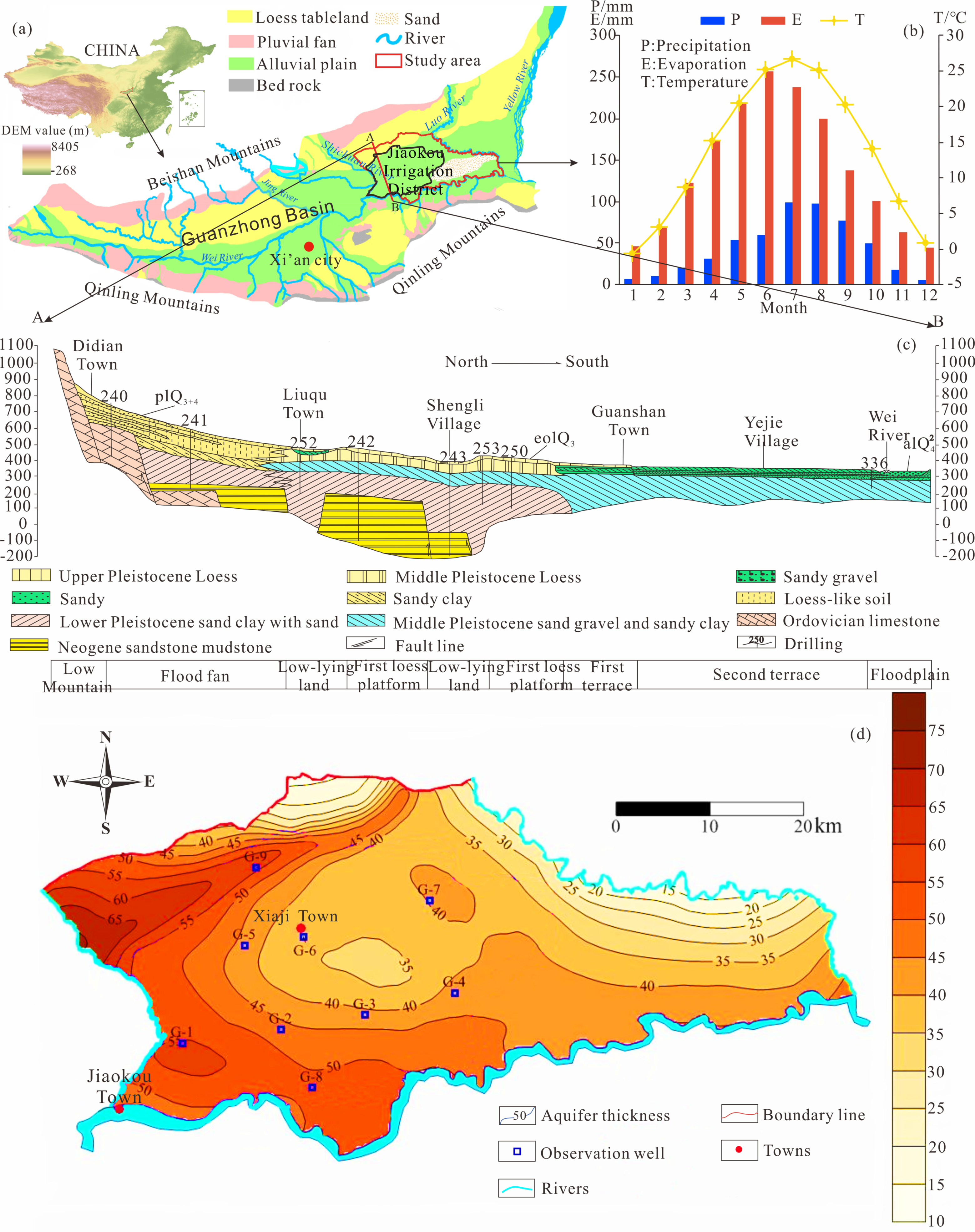
2.1. Study Area

2.1.1. Location and Climate

The study area (34°30′7″–34°52′37″N, 109°12′40″–110°10′1″E) with an area of 1895.57 km2 is situated in the eastern part of Guanzhong Basin, central China, approximately 60 km northeast of Xi’an (Figure 1). The Guanzhong Basin is located between the Beishan Mountains in the north and the Qinling Mountains in the south. The Wei River water system is the main source of surface water in the Guanzhong Basin. The Wei River flows through the central part of the Guanzhong Basin and is distributed in the south of Jiaokou Irrigation District. The length of Wei River in Shaanxi is 502.4 km, with catchment area of 67,108 km2, and the average annual runoff is 6.266 billion m3, which serves as the main source for the Jiaokou Irrigation District [8,19,25]. Additionally, the Shichuan River is distributed in the west of study area, while Luo River is in the east (Figure 1a). The Shichuan River has a total length of 137 km, an average decrease of 4.6‰, a catchment area of 4478 km2, and an annual runoff of 215 million m3, while the length of Luo River is 680.2 km, with an area of 26,905 km2 [54]. The climate of study area is warm temperate and semi-arid monsoon with a mean annual precipitation of 548.5 mm, annual evaporation of 1003.1 mm, and a mean annual air temperature of 13.4 °C. The meteorological details can be found in Table S1.

2.1.2. Geology and Hydrogeology

The Guanzhong Basin is part of the Fenwei fault basin, which is a typical Cenozoic faulted basin. It was formed at the end of the Cretaceous Period and the beginning of the Tertiary Period and was a product of the Himalayan Movement [54,55]. Cenozoic clastic rocks with a thickness of more than 6000 m have accumulated in the basin. The study area is primarily controlled by the Qinling zonal structure system. Its tectonic structure is an EW direction, which is the result of strong NS compression.
The main aquifer in the study area is the Quaternary strata, which are terrestrial deposits, the Primary covering the Tertiary, with only a small part overlying the Pre-Tertiary. Its thickness varies substantially and is controlled by factors, such as neotectonics movement and paleogeography. The maximum thickness of the Quaternary stratum ranges from 900 to 1200 m, while the minimum thickness is 300~400 m [19,20]. Additionally, the aquifers are continuously and widely distributed, and the groundwater flows from northwest to southeast. The different types of Quaternary sediments can be divided into two categories, namely, coarse-grained deposits dominated by gravel and pebbles and soil-like accumulations dominated by loess [54] (Figure 1).
The landform features of study area are an alluvial plain, loess tableland, and sand, which specifically includes five landscape types: floodplain, first terrace, and second terrace of the Wei River, loess plateau, and sand belt (Figure 1). The study area slopes to the southeast like a dustpan. The existence conditions and hydraulic characteristics indicate that the types of groundwater in the study area are primarily loose rock pore water and aeolian loess pore fissure water. The depth of groundwater is between 1 and 25 m, with the aquifer thickness ranging from 10 to 80 m (Figure 1).

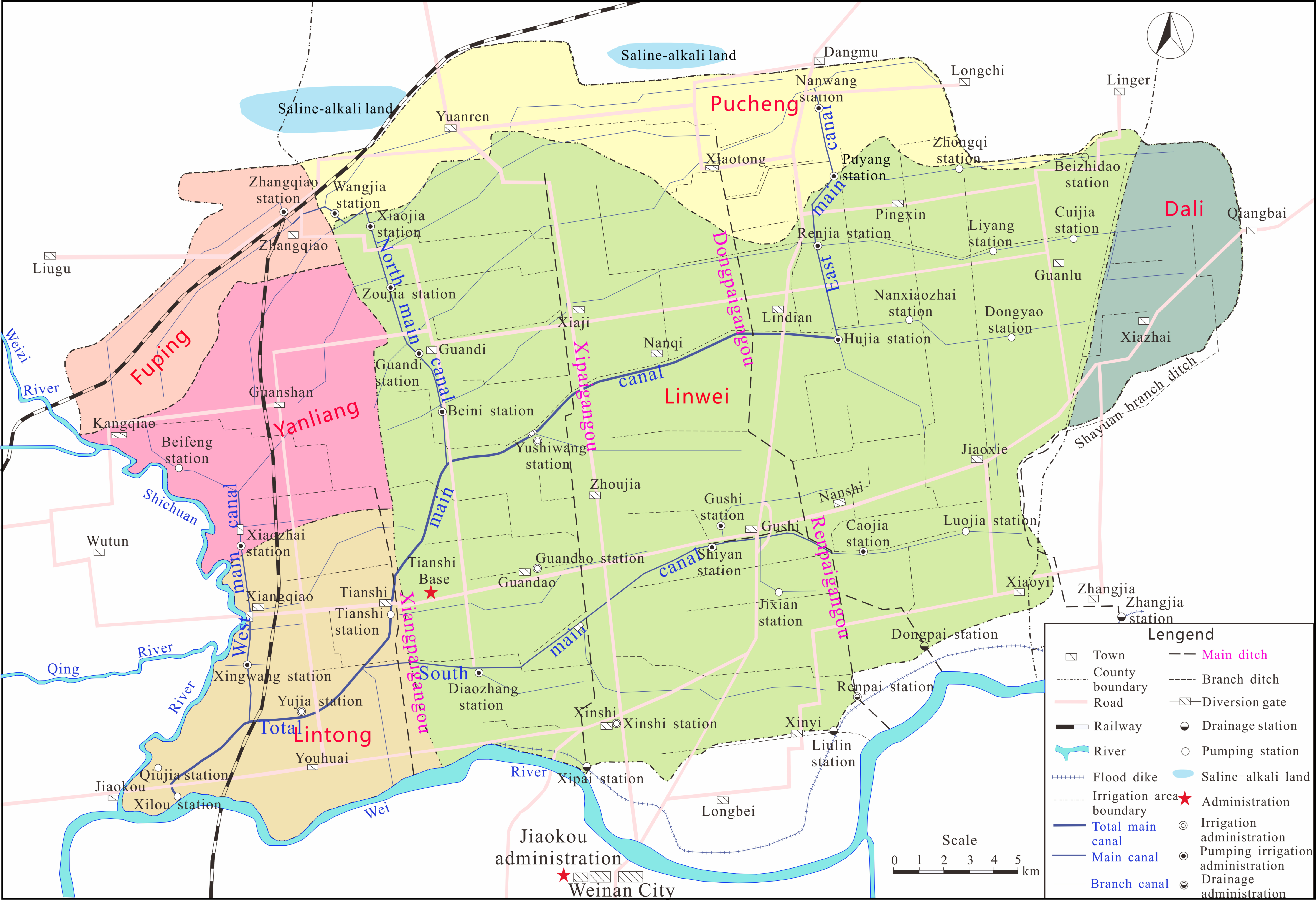
2.2. Aqueduct Distribution and Groundwater Exploitation

There are crisscross canals and drainage ditches within the Jiaokou Irrigation Area, including 5 main canals, 47 branch canals, 4 main ditches, and 56 branch ditches (Figure 2). Five main canals have a length of 95.84 km, and consist of the total main canal, east main canal, west main canal, south main canal, and north main canal, while 47 branch canals have a length of 328.77 km. Four main ditches are 86.77 km long, and 56 branch ditches are 346.48 km long [54].
Since the groundwater in the irrigation area is recharged by water that has leaked from irrigation, and the deeper the groundwater is buried, the higher the salinity. Shallow wells are used to make full use of the shallow groundwater to obtain sufficient water in the irrigation area. Currently, there are more than 3870 wells in the irrigation area with more than 3600 in normal use; the average annual irrigation area is 142 km2, with an average annual groundwater extraction volume of 43.469 million m3 [54]. Artificial pumping in the study area is primarily used for agricultural irrigation and consumption by rural humans and livestock. The amount of groundwater used for agricultural irrigation and consumption by humans and livestock was 502.3 million m3 and 0.0899 million m3, respectively.

2.3. Development and Calibration of the Model

2.3.1. Conceptual Model

The conceptual model includes system boundaries, hydrogeological characterization, and the flow system of groundwater [42]. Owing to the deep cutting and large water flow of the Wei and Luo Rivers, they are all generalized to the constant head boundary. The river level was obtained by linear interpolation based on the known river water level points. The Shichuan River is generalized as a river boundary owing to its shallow cutting and small water flow. The northern boundary is the front edge of the Fuping-Pucheng Plateau. Some of the groundwater flows into the area from the north side; thus, it is generalized as a specified flux boundary. The value of flow is calculated based on the phreatic flow direction, permeability coefficient, and aquifer thickness. It is added to the model in the form of a well. The drainage ditches in the simulation area are generalized as the third type of drainage ditches boundary because it has a hydraulic connection with the groundwater. In the vertical direction, the simulation area is a single phreatic aquifer. The upper boundary is the phreatic surface, and the lower boundary is the confining bed. The sources for the recharge of groundwater include precipitation, leakage from irrigation canals, irrigation infiltration, and lateral inflow. Evaporation, groundwater extraction, and discharge by drains are the major outflows. According to the “Evaluation Report of Groundwater Resources in Guanzhong Basin” [56] and the geological and geomorphological conditions of the simulation area, the hydraulic conductivity in the simulation area is determined (Figure 3).
The groundwater in the simulation area is affected by topography, landforms, and rivers. In the Loess Plateau in the northern part of simulation area, the phreatic water primarily flows from the northwest to southeast, while in the first and second terraces of the Wei River, phreatic water flows from the north to south into the Wei River. Additionally, on the east side of the simulation area, the groundwater flows from west to east into the Luo River, while on the west side, the groundwater tends to be discharged into the Shichuan River [8,19,20]. Simultaneously, owing to the influence of the drainage ditch, there is a local tendency to converge in the drainage ditch. However, in the vertical direction, there is basically no water exchange between the phreatic and confined water. Based on the analysis described above, the groundwater flow in the area is generalized with a plane two-dimensional unsteady flow.

2.3.2. Mathematical Model

Based on the hydrogeological conceptual model described above, the two-dimensional unsteady-state flow mathematical model of groundwater in the simulation area is shown in Equation (1).
x K h B h x + y K h B y + W = μ h t x ,   y D , t > 0
The initial and boundary conditions are as follows:
h ( x , y , 0 ) = h 0 ( x , y ) ( x , y ) D h ( x , y , t ) | Γ 1 = h 1 ( x , y ) t > 0 K h h n | Γ 2 = q t > 0 lim r r w r 0 2 π K h h r d θ = Q i t > 0 K h d h M A = Q d h d < h t > 0 , Drainage ditch
where D is the study areal extent; h is the groundwater head (m); h0 is the initial groundwater level (m); h1 is the water level of specified head boundary (m), i.e., providing a head distributed on the boundary; hd is the water level of drainage ditch (m); B is the elevation of confining bed (m); K is the hydraulic conductivity of aquifer (m/d); K’ is the hydraulic conductivity of silt layer at the bottom of the drainage ditch and canal (m/d); μ is the specific yield of phreatic aquifer sediments; M’ is the thickness at the bottom of the drainage ditch and canal (m); W is fluxes that represent recharge, evaporation, and pumping; A is the area of drainage ditch and canal; q is the single width flow of the specified flux boundary, i.e., providing the inbound (outbound) flow distribution on the boundary; r is the radial distance of pumping wells; Qi is the pumping volume of the i-th well; and n is the outer normal direction of the specified flux boundary.

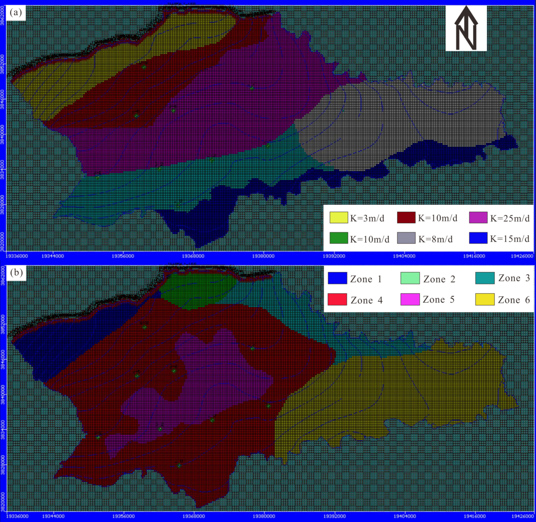
2.3.3. Model Construction

A two-dimensional unsteady flow hydrogeological model was developed to simulate the flow system in the Jiaokou Irrigation District using MODFLOW 2011.1. The study area (1895.57 km2) was discretized with a finite-difference gird comprising 301 columns, 141 rows, and a uniform cell dimension of 300 m × 300 m for the aquifer. In terms of time, the simulation area is divided into 12 stress periods with natural months as the unit. In this simulation, the water level measured in August 2013 was used to calibrate the model. To improve the calculation accuracy of the model, each stress period was divided further into 10 periods, and the time interval between adjacent periods is required to satisfy the following relationship:
t k + 1 = 1.2 t k
where tk is the k-th calculation period.
The digital elevation model of the simulation area is obtained by kriging spatial interpolation as shown in Figure 4a. The Wei and Luo Rivers were simulated with Constant Head in MODFLOW as described, while the Shichuan River was simulated with River boundary. Lateral recharge to aquifers from the northern boundaries was established as specified flux boundaries based on Darcy’s law, joining the model via a well boundary. The recharge is a superimposed result of precipitation, irrigation infiltration, canal leakage, and artificial pumping and was applied via the recharge boundary. Evaporation was introduced to the model with an evapotranspiration boundary, and the Extinction Depth is 5 m [19,54]. Discharge to the drains is represented in the model by drain boundaries. A no-flow boundary was established at the bottom of the aquifer.
The boundary conditions of the study area, average hydrology, meteorology, and water resources development and utilization data were added to the model, and the steady flow model was used for the operation to obtain the initial flow field of the model, as shown in Figure 4b. The WHS iteration method was selected for the model solution, and the maximum number of external iterations was set to 500, while the number of internal iterations was 250. The convergence standard for water level changes is 0.001 m, and the residual convergence standard is 0.0001 m.

2.3.4. Model Calibration

The model calibration was conducted using the piezometric data collected from September 2012 to August 2013, including precipitation, evaporation, groundwater extraction, water diversion and irrigation, and groundwater boundary conditions. The groundwater level in August 2013 was calculated based on the piezometric data, and the calculated water level was compared with the actual water level in August 2013. The parameters were adjusted repeatedly until the degree of fit met the requirements; i.e., the difference between the calculated and the observed groundwater level was <2 m [42]. The model can be used to simulate calculations in this area. The initial hydraulic parameters were adjusted during the calibration process. To test the accuracy of the model, the absolute residual mean (ARM), the normalized root mean square (NRMS), and the model efficiency (EF) were used in the MODFLOW software [24,57], for which the calculation formulae are as follows:
A R M = 1 N i = 1 N ( O i P i ) N R M S = 1 N i = 1 N ( O i P i ) 2 O i max O i min E F = i = 1 N ( O i m e a n ) 2 i = 1 N ( O i P i ) 2 i = 1 N ( O i m e a n ) 2
where Oi and Pi were the observed and predicted values, respectively, and N was the total number of observations. Mean was the average value of the observed groundwater levels.

2.3.5. Model Prediction

With MODFLOW calibrated, three hypothetical options for groundwater management were investigated (Figure 5). Scenario 1 considered using groundwater for spring and winter irrigation. Scenario 2 assumed that groundwater and surface water were used for irrigation, and the ratio was 2:1. Scenario 3 is a predictive model based on the Hanjiang–Wei River Water Diversion Project. The specific steps of each scenario are shown in Figure 5.

3. Results

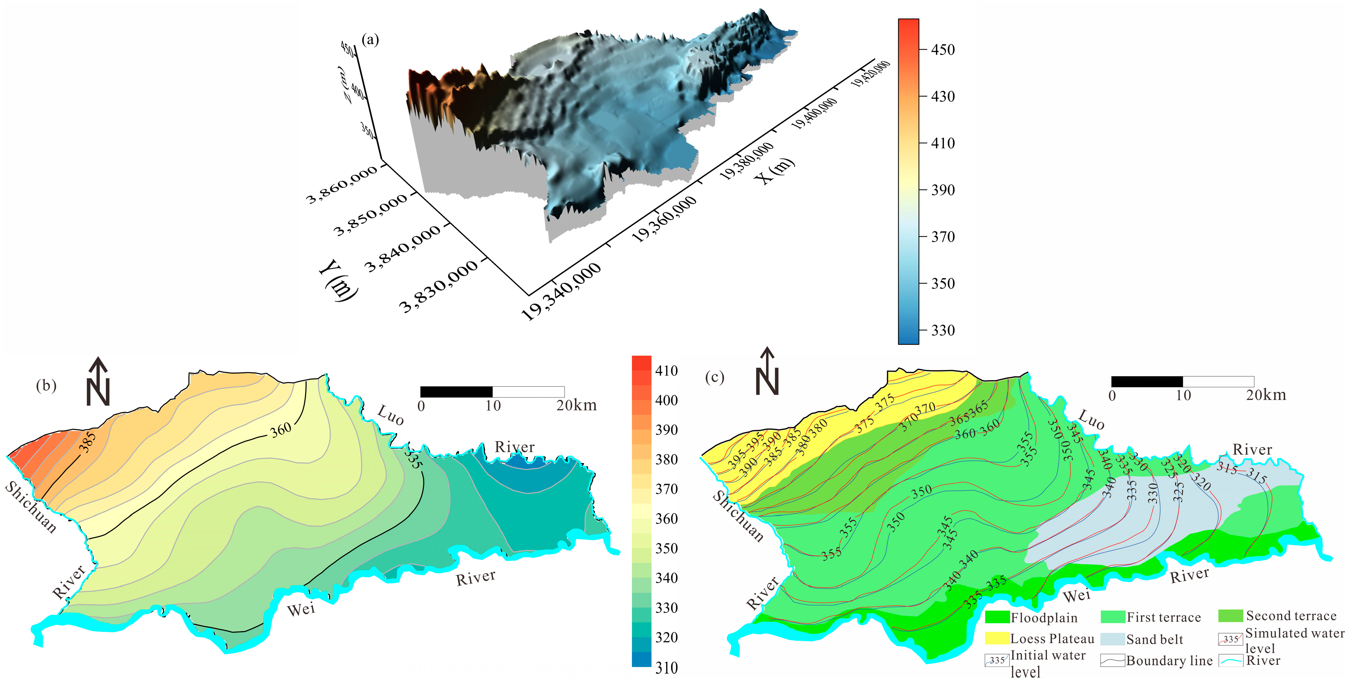
3.1. Calibration Results

The model has few errors and can substantially represent the state of groundwater movement [24]. The fitting result of the simulated value (red line) and observed value (blue line) of the groundwater flow field is shown in Figure 4c, which shows that the water level difference is basically within 1 m. The comparison from September 2012 to August 2013 based on the observation well’s date also confirmed this result. Moreover, the EF value is up to 0.99 (Supplementary Figure S1). Therefore, the established numerical model can meet the accuracy requirements of groundwater level simulation and prediction in the study area.

3.2. Groundwater Balance Analyses

Table 1 lists the results of the calculation of the groundwater balance. The total recharge of groundwater was 1.99 × 10⁸ m3/a in the operating results of the model as shown in the table. Among them, precipitation and canal leakage are the main resources to use to recharge the water. The amounts of recharge were 1.02 × 10⁸ m3/a and 0.65 × 10⁸ m3/a, comprising 51.26% and 32.81% of the total groundwater recharge, respectively. Irrigation infiltration and lateral runoff recharge comprised a relatively small proportion, comprising 12.56% and 3.37% of the total groundwater recharge, respectively.
In the meantime, the total discharge of groundwater was 1.93 × 10⁸ m3/a. The main discharge ways were lateral runoff and artificial pumping. The discharge amounts were 0.63 × 10⁸ m3/a and 0.61 × 10⁸ m3/a, comprising 32.64% and 31.61% of the total groundwater outflow, respectively. Evaporation followed and comprised 20.73% of the total outflow. The drainage ditch had the smallest outflow, comprising only 15.02% of the total outflow.

3.3. Annual Irrigation Water Demand and Supply in the Study Area

3.3.1. Annual Water Demand

In response to the problems faced in the study area, a reasonable plan to allocate water resources under the premise of meeting crop water requirements should be proposed. There are four main crops planted in the irrigation district, namely wheat, corn, cotton, and fruit trees [54]. Among them, the wheat, cotton, and fruit trees were summer crops, while the corn, cotton, and fruit trees were fall crops. Therefore, based on the irrigation quota of different crops in the irrigation district, the demand for water during the irrigation period was calculated, as shown in Table 2.

3.3.2. Annual Water Supply

Based on the research of Liu [54], the average water diversion volume at the head of the irrigation area was 21,142.71 × 104 m3/a for many years, and the utilization coefficient of the canal system was 0.51. Therefore, the water supply of the canal system during the irrigation period was Q = 21,142.71 × 104 m3/a × 0.51 = 10,782.78 × 104 m3/a. Additionally, the annual average groundwater pumping volume was 4,346.9 × 104 m3/a. Therefore, based on the monthly extraction of the canal system and groundwater in the irrigation area, a comparison table of crop water demand and water supply was obtained, as shown in Figure 6.
As shown in Figure 6, the total amount of irrigation water in a year is sufficient, and the irrigation water supply exceeded the demand for water for the crop. From a monthly perspective, spring irrigation (February, March, April, and May) and winter irrigation (January, November, and December) can meet the demand for water, but the supply of water for irrigation in the summer is insufficient. The amount of water available in June is insufficient, and the volume of water shortage was 667.7406 × 10⁴ m3, while the comparable value for July was 75.7603 × 10⁴ m3. There are two main reasons for this situation. On the one hand, owing to the insufficient flow of the Wei River, and alternatively, owing to the large amount of sand in the river, the head of the canal cannot be started for water diversion, resulting in an insufficient diversion of water.

4. Discussion

4.1. Scenario 1: Primarily Using Groundwater for Spring and Winter Irrigation

For this scenario, the plan for the allocation of water resources is shown in Table S3. Irrigation water can be added to the model with a recharge module and run in an unsteady flow for 50 years. The decrease in water level and the buried depth after 50 years is shown in Figure 7a and 7b, respectively.
The groundwater level draws down in a funnel shape as shown in Figure 7a. The deepest decrease in the north-central part of the irrigation area was 25 m, and it spread around. The decrease in water level is only less than 5 m in the river area and the eastern part of the study area. In terms of burial depth, with the exception of the floodplain of Wei River, the burial depths of the water levels were all greater than 20 m (Figure 7b). However, when the water level decreases by more than one-half of the thickness of the aquifer, it will cause problems, such as difficulty in mining and the deterioration of water quality [58]. The thickness of the aquifer in the Jiaokou Irrigation District varies from 30 to 50 m (Figure 1). Therefore, to protect the groundwater source, the maximum decrease in water level should be maintained within 15 m. However, in scenario 1, the maximum drawdown (above 25 m) is beyond this limit, indicating that the scheme is unsustainable.

4.2. Scenario 2: The Ratio of Groundwater to Surface Water Is 2:1 for Irrigation

For this scenario, the plan for the allocation of water resources is shown in Table S4. As in scenario 1, the irrigation water was added to the model with a recharge module and run in an unsteady flow for 50 years. The decrease in water level and buried depth after 50 years is shown in Figure 8a and 8b, respectively, and the groundwater drawdown in the observation wells is shown in Table S5.
As shown in Figure 8a, the largest decrease in water level occurred in the northwest and northeast regions of the irrigation district and was approximately 10 m. The buried depth of the water level was basically between 5 and 30 m (Figure 8b), which will not result in harm by salinization. Simultaneously, according to the field survey in 2013, the wells used for irrigation in the study area are basically more than 40 m deep [54]; thus, the buried depth of 5–30 m can meet the requirements for providing water.
As shown in Table S5, the water level decreases of the observation wells were all within 15 m, and the largest decrease was 10.13 m, which is in the G-9 observation well. Followed by G-7 and G-5, the water level decrease was 7.16 and 6.50 m, respectively. The minimum water level decrease was 1.71 m, which was in the G-1 observation well. The G-9, G-7, and G-5 observation wells with the large decrease in water level should be selected, and a line of decrease in water level over time drawn, as shown in Figure 9. This figure indicates that the water levels of observation wells G-9, G-7, and G-5 basically stabilized after 50 years. Combined with the decrease in water level and the change in trend of the water level, scenario 2 appears to be reasonably sustainable. If the water quality of the Wei River maintains its current status, scenario 2 can be used for the allocation of groundwater and surface water.

4.3. Scenario 3: Predictive Model Based on the Hanjiang-to-Weihe River Valley Water Diversion Project

To adapt to the contradiction between the supply and demand of water resources in the Guanzhong Basin and improve the ecological environment of the Wei River, the Shaanxi Provincial Government planned the Hanjiang-to-Weihe River Valley Water Diversion Project in 2008 [54]. The project supplements the water supply of Xi’an, Xianyang, Weinan, and Tongchuan by diverting water from Hanjiang, thereby returning the ecological water of Wei River and helping to improve the water quality of Wei River. The Hanjiang-to-Weihe River Valley Water Diversion Project was planned in three phases. The third phase of the project will be completed in 2030, and it is estimated that 15 × 108 m3 of water will be transferred [54]. Combining with the characteristics and development trend of the project, a long-term predictive plan for the irrigation district is proposed.
(1)
This scenario assumes that the water quality of the Wei River will recover after the Hanjiang-to-Weihe River Valley Water Diversion Project starts operation for 10 years (year 2040).
In the early stage of water level restoration, i.e., before 2040, the allocation of water resources is the same as that in scenario 2. After 2040, the plans to allocate surface water and groundwater are shown in Table S6. When the model is run in an unsteady flow, the decrease in water level after 20 years was basically within 1 m with the exception of a few places compared with the initial water level as shown in Figure 10a. This indicates that the groundwater level has basically been restored.
(2)
This scenario assumes that the water quality of Wei River will recover after the Hanjiang-to-Weihe River Valley Water Diversion Project starts operation in 20 years (year 2050).
Similar to the previous example, during the early stage of restoration of the water level, i.e., before 2050, the allocation of water resources was the same as in scenario 2. After 2050, the plans to allocate surface water and groundwater are the same as in Table S6. When the model is run in an unsteady flow, after 30 years, the decrease in groundwater level was basically within 1 m of the initial water level, with the exception of a few places in the north of the study area, indicating that the groundwater level had basically been recovered at this time. The decrease in water level after 30 years is shown in Figure 10b.
The water in the drainage ditch in the study area contains high salt content. The maximum value exceeds 10 g/L and the annual average salt content is 2.33 g/L (Supplementary Figure S2). The shallow burial depth of the groundwater resulting from long-term irrigation and the strong evaporation increases the salinity of groundwater, which leads to the high salinity of water in the drainage ditch. Therefore, drainage water is not suitable for use in general, but only suitable for irrigation of salt-tolerant crops. To prevent the secondary salinization caused by an excessive increase in the groundwater level owing to a large amount of surface water irrigation, after the groundwater level has been restored, a new plan to allocate the water resource needs to be provided. Therefore, based on the allocation plan after the water level had been restored and combined with the demand for water from the crops, a new plan to allocate water resources is proposed, as shown in Table S7. Compared with the plan for allocation after the restoration of the water level, the plan had two adjustments. The first one was an increase in the exploitation of groundwater sources during the summer irrigation period to ensure the water requirements of crops. Secondly, during spring irrigation and winter irrigation, the amount of water diversion at the head of the canal was reduced. The model was run for 50 years based on this plan to allocate water resources, and the decrease in water level and buried depth after 50 years are shown in Figure 11a and 11b, respectively. As shown in Figure 11a, the groundwater level had decreased to some extent, and the maximum decrease was approximately 5 m. This is primarily because the plan to allocate water increased the amount of groundwater extraction and reduced the amount of surface water diversion. Moreover, the buried depth of the groundwater level had also increased to basically above 3 m (Figure 11b), which meets its requirements for the critical depth. It is worth noting that the maximum critical depth is 2.8 m. According to Jin [59], the critical depth of the study area is calculated, and the specific calculation process is shown in the Supplementary Materials.
In the meantime, the water level changes in the observation wells are shown in Table S8. It is apparent that the largest decrease was 4.55 m, followed by 2.91 m and 2.79 m, which correspond to G-9, G-5, and G-7, respectively. Therefore, the G-9, G-7, and G-5 observation wells were selected to study the trend of water level changes, as shown in Figure 12. At first, the water level will decrease, then slowly decrease, and finally, stabilize. Combined with the decrease in water level map after 50 years, the water level will decrease slightly when the water resources are allocated with this scheme, and remain within an acceptable amount of decrease. The final water level will stabilize and reach a new equilibrium state. Combined with the changes in the buried depth of the groundwater level, the decrease in water level will render the buried depth of the groundwater greater than the critical buried depth (2.8 m); thus, it will not result in salinization. Therefore, the scheme described above is reasonable and feasible.

5. Conclusions

The present study highlighted the close association between water allocation and groundwater level decline in the irrigation area. A two-dimensional unsteady flow model was constructed and calibrated. Moreover, three scenarios were established to discuss the problems of water shortage and groundwater quality caused by water level drop.
(1)
The model results show that the groundwater in the study area is in a positive equilibrium and the total recharge and discharge of groundwater were 1.99 × 10⁸ m3/a and 1.93 × 10⁸ m3/a, respectively. It is noted that summer is short of water.
(2)
For scenario 1, when the groundwater is primarily used for irrigation, the water level in most areas decreases significantly after 50 years, reaching 25 m at the maximum, and the buried depth is basically above 20 m.
(3)
For scenario 2, when the ratio of groundwater to surface water is 2:1 for irrigation, the largest decrease in water level is approximately 10 m, and the buried depth of the water level is basically between 5 and 30 m, indicating that scenario 2 is reasonably feasible to solve the scarcity of water.
(4)
The results of scenario 3 indicate that the maximum decrease is approximately 5 m, and the buried depth of the groundwater level is basically above 3 m. It can be seen that the joint regulation of groundwater and surface water and the Hanjiang-to-Weihe River Valley Water Diversion Project have significant optimization benefits for groundwater level change and soil salinization in irrigation areas.
Therefore, model results were useful and valuable to protect water resources and prevent water pollution and provide a reference to rationally allocate water resources for other irrigation districts in arid and semi-arid areas. Regrettably, the capacity of groundwater to transport pollution was not examined in this study. Therefore, it will be the goal of future research.

Supplementary Materials

The following supporting information can be downloaded at: https://www.mdpi.com/article/10.3390/rs15030571/s1, Figure S1: Observed and simulated groundwater levels at the monitoring wells. The insets depict temporal variations over one year in calculated water levels (green lines) as compared to field measurements (red lines) at 9 selected observation wells. Water levels are shown in meters (m) above sea level; Figure S2: Change in salt discharge from drains in the study area from 2015 to 2020; Table S1: Statistical results of meteorological data in the study area; Table S2: The recharge parameter values of groundwater in the model; Table S3: Groundwater and surface water allocation for scenario 1; Table S4: Groundwater and surface water allocation for scenario 2; Table S5: Observation well water level changes in 50 years for scenario 2; Table S6: Water resources allocation plan during the water level restoration period; Table S7: Water resources allocation plan after water level restoration for predictive model (scenario 3); Table S8: Observation well water level changes in 50 years for scenario 3; Additional supplementary material: The specific calculation process of the critical depth.

Author Contributions

Conceptualization, H.Q. and Q.Z.; Data curation, Q.Z. and P.X.; Formal analysis, Q.Z. and P.X.; Funding acquisition, H.Q.; Methodology, Q.Z.; Software, Q.Z., R.L. and X.K.; Supervision, H.Q. and R.L.; Writing—original draft preparation, Q.Z.; Writing—review and editing, H.Q., A.F. and J.S. All authors have read and agreed to the published version of the manuscript.

Funding

We are grateful for the support from the National Natural Science Foundation of China (41931285 and 41790441) and the Program of Introducing Talents of Discipline to Universities (B08039).

Data Availability Statement

The data of this article is unavailable due to privacy or ethical restrictions.

Acknowledgments

The completion of this article was inseparable from the contributions of all authors. Their support is gratefully acknowledged.

Conflicts of Interest

The authors declare no conflict of interest.

References

  1. Qin, J.; Duan, W.; Chen, Y.; Dukhovny, V.A.; Sorokin, D.; Li, Y.; Wang, X. Comprehensive evaluation and sustainable development of water–energy–food–ecology systems in Central Asia. Renew. Sustain. Energy Rev. 2022, 157, 112061. [Google Scholar] [CrossRef]
  2. Luo, P.P.; Zheng, Y.; Wang, Y.Y.; Zhang, S.P.; Yu, W.Q.; Zhu, X.; Huo, A.D.; Wang, Z.H.; He, B.; Nover, D. Comparative Assessment of Sponge City Constructing in Public Awareness, Xi’an, China. Sustainability 2022, 14, 11653. [Google Scholar] [CrossRef]
  3. Zhu, W.; Zha, X.; Luo, P.; Wang, S.; Cao, Z.; Lyu, J.; Zhou, M.; He, B.; Nover, D. A quantitative analysis of research trends in flood hazard assessment. Stoch. Environ. Res. Risk Assess. 2022, 37, 413–428. [Google Scholar] [CrossRef]
  4. Wang, Z.; Luo, P.P.; Zha, X.B.; Xu, C.Y.; Kang, S.X.; Zhou, M.M.; Nover, D.; Wang, Y.H. Overview assessment of risk evaluation and treatment technologies for heavy metal pollution of water and soil. J. Clean. Prod. 2022, 379, 134043. [Google Scholar] [CrossRef]
  5. Han, D.M.; Song, X.F.; Currell, M.J.; Cao, G.L.; Zhang, Y.H.; Kang, Y.H. A survey of groundwater levels and hydrogeochemistry in irrigated fields in the Karamay Agricultural Development Area, northwest China: Implications for soil and groundwater salinity resulting from surface water transfer for irrigation. J. Hydrol. 2011, 405, 217–234. [Google Scholar] [CrossRef]
  6. Nong, X.Z.; Shao, D.G.; Zhong, H.; Liang, J.K. Evaluation of water quality in the South-to-North Water Diversion Project of China using the water quality index (WQI) method. Water Res. 2020, 178, 115781. [Google Scholar] [CrossRef]
  7. Zhang, Q.Y.; Xu, P.P.; Qian, H. Groundwater Quality Assessment Using Improved Water Quality Index (WQI) and Human Health Risk (HHR) Evaluation in a Semi-arid Region of Northwest China. Expo. Health 2020, 12, 487–500. [Google Scholar] [CrossRef]
  8. Zhang, Q.Y.; Xu, P.P.; Chen, J.; Qian, H.; Qu, W.G.; Liu, R. Evaluation of groundwater quality using an integrated approach of set pair analysis and variable fuzzy improved model with binary semantic analysis: A case study in Jiaokou Irrigation District, east of Guanzhong Basin, China. Sci. Total Environ. 2021, 767, 145247. [Google Scholar] [CrossRef]
  9. Dehghanipoura, A.H.; Schoups, G.; Zahabiyoun, B.; Babazadeh, H. Meeting agricultural and environmental water demand in endorheic irrigated river basins: A simulation-optimization approach applied to the Urmia Lake basin in Iran. Agric. Water Manag. 2020, 241, 106353. [Google Scholar] [CrossRef]
  10. Mostaza-Colado, D.; Carreño-Conde, F.; Rasines-Ladero, R.; Iepure, S. Hydrogeochemical characterization of a shallow alluvial aquifer: 1 baseline for groundwater quality assessment and resource management. Sci. Total Environ. 2018, 639, 1110–1125. [Google Scholar] [CrossRef]
  11. Singh, A. Simulation-optimization modeling for conjunctive water use management. Agric. Water Manag. 2014, 141, 23–29. [Google Scholar] [CrossRef]
  12. Liu, W.; Park, S.; Bailey, R.T.; Molina-Navarro, E.; Andersen, H.E.; Thodsen, H.; Nielsen, A.; Jeppesen, E.; Jensen, J.S.; Jensen, J.B.; et al. Quantifying the streamflow response to groundwater abstractions for irrigation or drinking water at catchment scale using SWAT and SWAT–MODFLOW. Environ. Sci. Eur. 2020, 32, 113. [Google Scholar] [CrossRef]
  13. Ni, X.J.; Parajuli, P.B.; Ouyang, Y. Assessing Agriculture Conservation Practice Impacts on Groundwater Levels at Watershed Scale. Water Resour. Manag. 2020, 34, 1553–1566. [Google Scholar] [CrossRef]
  14. Xue, J.; Gui, D.; Lei, J.; Sun, H.; Zeng, F.; Feng, X. A hybrid Bayesian network approach for trade-offs between environmental flows and agricultural water using dynamic discretization. Adv. Water Resour. 2017, 110, 445–458. [Google Scholar] [CrossRef]
  15. Peng, J.B.; Sun, X.H.; Wang, W.; Sun, G.C. Characteristics of land subsidence, earth fissures and related disaster chain effects with respect to urban hazards in Xi’an, China. Environ. Earth Sci. 2016, 75, 15. [Google Scholar] [CrossRef]
  16. Jia, Z.J.; Qiao, J.W.; Peng, J.B.; Lu, Q.Z.; Xia, Y.Y.; Zang, M.D.; Wang, F.Y.; Zhao, J.Y. Formation of ground fissures with synsedimentary characteristics: A case study in the Linfen Basin, northern China. J. Asian Earth Sci. 2021, 214, 104790. [Google Scholar] [CrossRef]
  17. Bagheri-Gavkosh, M.; Hosseini, S.M.; Ataie-Ashtiani, B.; Sohani, Y.; Ebrahimian, H.; Morovat, F.; Ashra, S. Land subsidence: A global challenge. Sci. Total Environ. 2021, 778, 146193. [Google Scholar] [CrossRef]
  18. Li, H.J.; Zhu, L.; Guo, G.X.; Zhang, Y.; Dai, Z.X.; Li, X.J.; Chang, L.Z.; Teatini, P. Land subsidence due to groundwater pumping: Hazard probability assessment through the combination of Bayesian model and fuzzy set theory. Nat. Hazards Earth Syst. Sci. 2021, 21, 823–835. [Google Scholar] [CrossRef]
  19. Zhang, Q.Y.; Xu, P.P.; Qian, H.; Yang, F.X. Hydrogeochemistry and fluoride contamination in Jiaokou Irrigation District, Central China: Assessment based on multivariate statistical approach and human health risk. Sci. Total Environ. 2020, 741, 140460. [Google Scholar] [CrossRef]
  20. Zhang, Q.Y.; Qian, H.; Xu, P.P.; Li, W.Q.; Feng, W.W.; Liu, R. Effect of hydrogeological conditions on groundwater nitrate pollution and human health risk assessment of nitrate in Jiaokou Irrigation District. J. Clean. Prod. 2021, 298, 126783. [Google Scholar] [CrossRef]
  21. Noori, R.; Hooshyaripor, F.; Javadi, S.; Dodangeh, M.; Tian, F.Q.; Adamowski, J.F.; Berndtsson, R.; Baghvand, A.; Klöve, B. PODMT3DMS-Tool: Proper orthogonal decomposition linked to the MT3DMS model for nitrate simulation in aquifers. Hydrogeol. J. 2020, 28, 1125–1142. [Google Scholar] [CrossRef]
  22. Chen, J.; Qian, H.; Gao, Y.Y.; Wang, H.K.; Zhang, M.S. Insights into hydrological and hydrochemical processes in response to water replenishment for lakes in arid regions. J. Hydrol. 2020, 581, 124386. [Google Scholar] [CrossRef]
  23. Wu, X.; Xia, J.; Zhan, C.S.; Jia, R.L.; Li, Y.; Qiao, Y.F.; Zou, L. Modeling soil salinization at the downstream of a lowland reservoir. Hydrol. Res. 2019, 50, 1202–1215. [Google Scholar] [CrossRef]
  24. Yang, G.; Tian, L.J.; Li, X.L.; He, X.L.; Gao, Y.L.; Li, F.D.; Xue, L.Q.; Li, P.F. Numerical assessment of the effect of water-saving irrigation on the water cycle at the Manas River Basin oasis, China. Sci. Total Environ. 2020, 707, 135587. [Google Scholar] [CrossRef] [PubMed]
  25. Zhang, Q.Y.; Qian, H.; Xu, P.P.; Hou, K.; Yang, F.X. Groundwater quality assessment using a new integrated-weight water quality index (IWQI) and driver analysis in the Jiaokou Irrigation District, China. Ecotox. Environ. Saf. 2021, 212, 111992. [Google Scholar] [CrossRef] [PubMed]
  26. Guevara-Ochoa, C.; Medina-Sierra, A.; Vives, L. Spatio-temporal effect of climate change on water balance and interactions between groundwater and surface water in plains. Sci. Total Environ. 2020, 722, 137886. [Google Scholar] [CrossRef]
  27. Klaas, D.K.S.Y.; Imteaz, M.A.; Sudiayem, I.; Klaas, E.M.E.; Klaas, E.C.M. Assessing climate changes impacts on tropical karst catchment: Implications on groundwater resource sustainability and management strategies. J. Hydrol. 2020, 582, 124426. [Google Scholar] [CrossRef]
  28. Wang, S.; Cao, Z.; Luo, P.; Zhu, W. Spatiotemporal Variations and Climatological Trends in Precipitation Indices in Shaanxi Province, China. Atmosphere 2022, 13, 744. [Google Scholar] [CrossRef]
  29. Chang, S.W.; Chung, I.-M.; Kim, M.G.; Yifru, B.A. Vulnerability assessment considering impact of future groundwater exploitation on coastal groundwater resources in northeastern Jeju Island, South Korea. Environ. Earth Sci. 2020, 79, 498. [Google Scholar] [CrossRef]
  30. Mohseni, N.; Bol, R. Variation in the rate of land subsidence induced by groundwater extraction and its effect on the response pattern of soil microbial communities. Earth Surf. Proc. Landf. 2021, 46, 1898–1908. [Google Scholar] [CrossRef]
  31. Zhu, Y.; Luo, P.; Su, F.; Zhang, S.; Sun, B. Spatiotemporal Analysis of Hydrological Variations and Their Impacts on Vegetation in Semiarid Areas from Multiple Satellite Data. Remote Sens. 2020, 12, 4177. [Google Scholar] [CrossRef]
  32. Omar, P.J.; Gaur, S.; Dwivedi, S.B.; Dikshit, P.K.S. A Modular Three-Dimensional Scenario-Based Numerical Modelling of Groundwater Flow. Water Res. Manag. 2020, 34, 1913–1932. [Google Scholar] [CrossRef]
  33. Luo, P.P.; Luo, M.T.; Li, F.Y.; Qi, X.G.; Huo, A.D.; Wang, Z.H.; He, B.; Takara, K.; Nover, D.; Wang, Y.H. Urban flood numerical simulation: Research, methods and future perspectives. Environ. Model. Softw. 2022, 156, 105478. [Google Scholar] [CrossRef]
  34. Wang, S.T.; Luo, P.P.; Xu, C.Y.; Zhu, W.; Cao, Z.; Ly, S. Reconstruction of Historical Land Use and Urban Flood Simulation in Xi’an, Shannxi, China. Remote Sens. 2022, 14, 6067. [Google Scholar] [CrossRef]
  35. Butts, M.; Graham, D. Evolution of an integrated surface water-groundwater hydrological modelling system. In Proceedings of the IAHR International Groundwater Symposium—Flow and Transport in Heterogeneous Subsurface Formations: Theory, Modelling & Applications, Istanbul, Turkey, 18–20 June 2008. [Google Scholar]
  36. DHI. MIKE SHE User Manual; DHI—Water and Environment: Hørsholm, Denmark, 2007. [Google Scholar]
  37. Jones, J.P.; Sudicky, E.A.; McLaren, R.G. Application of a fully-integrated surface-subsurface flow model at the watershed-scale: A case study. Water Resour. Res. 2008, 44, 1–13. [Google Scholar] [CrossRef]
  38. Ran, Q.H.; Chen, X.X.; Hong, Y.Y.; Ye, S.; Gao, J.H. Impacts of terracing on hydrological processes: A case study from the Loess Plateau of China. J. Hydrol. 2020, 588, 125045. [Google Scholar] [CrossRef]
  39. Hwang, H.T.; Jeen, S.W.; Kaown, D.; Lee, S.S.; Sudicky, E.A.; Steinmoeller, D.T.; Lee, K.K. Backward probability model for identifying multiple contaminant source zones under transient variably saturated flow conditions. Water Resour. Res. 2020, 56, e2019WR025400. [Google Scholar] [CrossRef]
  40. Persaud, E.; Levison, J.; MacRitchie, S.; Berg, S.J.; Erler, A.R.; Parker, B.; Sudicky, E. Integrated modelling to assess climate change impacts on groundwater and surface water in the Great Lakes Basin using diverse climate forcing. J. Hydrol. 2020, 584, 124682. [Google Scholar] [CrossRef]
  41. Deng, C.; Bailey, R.T. Assessing causes and identifying solutions for high groundwater levels in a highly managed irrigated region. Agric. Water Manag. 2020, 240, 106329. [Google Scholar] [CrossRef]
  42. Qian, H.; Chen, J.; Howard, K.W.F. Assessing groundwater pollution and potential remediation processes in a multi-layer aquifer system. Environ. Pollut. 2020, 263, 114669. [Google Scholar] [CrossRef]
  43. Tran, Q.Q.; Meert, P.; Huysmans, M.; Willems, P. On the importance of river hydrodynamics in simulating groundwater levels and baseflows. Hydrol. Process. 2020, 34, 1754–1767. [Google Scholar]
  44. Xiang, Z.C.; Bailey, R.T.; Nozari, S.; Husain, Z.; Kisekka, I.; Sharda, V.; Gowda, P. DSSAT-MODFLOW: A new modeling framework for exploring groundwater conservation strategies in irrigated areas. Agric. Water Manag. 2020, 232, 106033. [Google Scholar] [CrossRef]
  45. Stefania, G.A.; Rotiroti, M.; Fumagalli, L.; Simonetto, F.; Capodaglio, P.; Zanotti, C.; Bonomi, T. Modeling groundwater/surface-water interactions in an Alpine valley (the Aosta Plain, NW Italy): The effect of groundwater abstraction on surface-water resources. Hydrogeol. J. 2018, 26, 147–162. [Google Scholar] [CrossRef]
  46. Javadi, S.; Saatsaz, M.; Shahdany, S.M.H.; Neshat, A.; Milan, S.G.; Akbari, S. A new hybrid framework of site selection for groundwater recharge. Geosci. Front. 2021, 12, 101144. [Google Scholar] [CrossRef]
  47. Mirlas, V. Assessing soil salinity hazard in cultivated areas using MODFLOW model and GIS tools: A case study from the Jezre’el Valley, Israel. Agric. Water Manag. 2012, 109, 144–154. [Google Scholar] [CrossRef]
  48. Mirlas, V.; Kulagin, V.; Ismagulova, A.; Anker, Y. MODFLOW and HYDRUS Modeling of Groundwater Supply Prospect Assessment for Distant Pastures in the Aksu River Middle Reaches. Sustainability 2022, 14, 16783. [Google Scholar] [CrossRef]
  49. Duan, W.; Zou, S.; Christidis, N.; Schaller, N.; Chen, Y.; Sahu, N.; Li, Z.; Fang, G.H.; Zhou, B.T. Changes in temporal inequality of precipitation extremes over China due to anthropogenic forcings. NPJ Clim. Atmos. Sci. 2022, 5, 33. [Google Scholar] [CrossRef]
  50. Du, X.Z.; Dong, L.H.; Kang, W.J. Research on ecological product value realization mechanism in water diversion regions of Hanjiang-to-Weihe River Valley Water Diversion Project. Water Conserv. Constr. Manag. 2021, 41, 6–11+5. (In Chinese) [Google Scholar]
  51. Jin, Y.; Xu, G.X.; Qiao, H.J.; Dong, L.H.; Tan, Q.L. Research on the ecological compensation mechanism of the water source protection area of the Hanjiang-to-Weihe River Valley Water Diversion Project. Water Resour. Dev. Res. 2021, 21, 50–55. (In Chinese) [Google Scholar]
  52. Li, M.; Ge, D.Q.; Liu, B.; Zhang, L.; Wang, Y.; Guo, X.F.; Wang, Y.; Zhang, D.D. Research on development characteristics and failure mechanism of land subsidence and ground fissure in Xi’an, monitored by using time-series SAR interferometry. Geomat. Nat. Hazards Risk 2019, 10, 699–718. [Google Scholar] [CrossRef] [Green Version]
  53. Gao, C.; Ren, M.Z.; Liu, D.F.; Huang, Q. Risk evaluation of multi-objective dispatching scheme for Shaanxi Hangjiang-to-Weihe River Valley Water Diversion Project. Pearl River 2020, 41, 81–87. (In Chinese) [Google Scholar]
  54. Liu, R. Study on the Rational Allocation of Water Resources in Jiaokou Irrigation District; Chang’an University: Xi’an, China, 2014. (In Chinese) [Google Scholar]
  55. Xu, P.P.; Feng, W.W.; Qian, H.; Zhang, Q.Y. Hydrogeochemical characterization and irrigation quality assessment of shallow groundwater in the Central-Western Guanzhong Basin, China. Int. J. Environ. Res. Public Health 2019, 16, 1492. [Google Scholar] [CrossRef] [Green Version]
  56. Shaanxi Geological Survey Institute. Evaluation Report of Groundwater Resources in Guanzhong Basin; Shaanxi Geological Survey Institute: Xi’an, China, 2002. (In Chinese) [Google Scholar]
  57. Lyu, S.; Chen, W.P.; Wen, X.F.; Chang, A.C. Integration of HYDRUS-1D and MODFLOW for evaluating the dynamics of salts and nitrogen in groundwater under long-term reclaimed water irrigation. Irrig. Sci. 2019, 37, 35–47. [Google Scholar] [CrossRef]
  58. Zhang, C.C.; Shao, J.L.; Li, C.J.; Cui, Y.L. Research on groundwater ecological environment water level in north China plain. J. Jilin Univ. (Earth Sci. Ed.) 2003, 33, 323–326. (In Chinese) [Google Scholar]
  59. Jin, J. Study on Early Warning of Groundwater Environment under Papermaking Wastewater Irrigation Condition; Chang’an University: Xi’an, China, 2013. (In Chinese) [Google Scholar]
Figure 1. Study area map showing (a) locations and geomorphology, (b) meteorological elements, including precipitation (P), evaporation (E), and temperature (T), (c) stratigraphic profile, and (d) aquifer thickness.
Remotesensing 15 00571 g001
Figure 2. Map of the distribution of canal system and drainage ditches in the Jiaokou Irrigation District.
Remotesensing 15 00571 g002
Figure 3. Maps that show the model parameter partition: (a) hydraulic conductivity; (b) recharge area map. See Table S2 for the specific assignment of recharge.
Remotesensing 15 00571 g003
Figure 4. (a) Digital elevation model of ground surface in the simulation area; (b) The initial head diagram of the study area; (c) Comparison chart between the model running results and actual measured water level above mean sea level.
Remotesensing 15 00571 g004
Figure 5. Model simulations—scenarios 1, 2, and 3.
Remotesensing 15 00571 g005
Figure 6. The relationship between crop water demand and supply.
Remotesensing 15 00571 g006
Figure 7. Maps that show the (a) decrease in water level and (b) buried depth after 50 years for scenario 1.
Remotesensing 15 00571 g007
Figure 8. Maps showing the (a) decrease in water level and (b) buried depth after 50 years for scenario 2.
Remotesensing 15 00571 g008
Figure 9. Maps showing the trend in change in water level of (a) G-5, (b) G-7, and (c) G-9 observation well for scenario 2.
Remotesensing 15 00571 g009
Figure 10. The decrease in groundwater level after (a) 20 years and (b) 30 years of water level restoration.
Remotesensing 15 00571 g010
Figure 11. Maps that show the (a) decrease in water level and (b) buried depth after 50 years for scenario 3.
Remotesensing 15 00571 g011
Figure 12. Maps that show the trend in change in the water level of (a) G-5, (b) G-7, and (c) G-9 observation wells for scenario 3.
Remotesensing 15 00571 g012
Table 1. Groundwater balance calculation results of MODFLOW model.
RechargeWater Volume (108 m3/a)PercentageDischargeWater Volume (108 m3/a)Percentage
Precipitation1.0251.26%Lateral runoff (out)0.6332.64%
Canal leakage0.6532.81%Pumping0.6131.61%
Irrigation infiltration0.2512.56%Evaporation0.4020.73%
Lateral runoff (in)0.073.37%Drainage ditch0.2915.02%
Total1.99100%Total1.93100%
Equilibrium difference0.06
Relative equilibrium difference3.1%
Table 2. Monthly water demand during the irrigation period.
MonthWater Demand (104 m3)Total
WheatCornCottonOrchard
1339.90 339.90
2642.20 642.20
31153.70 1153.70
41684.85 59.64600.522345.00
52170.37 76.83652.802900.00
6 1867.0885.88742.252695.20
7 1575.3478.54449.322103.20
8 1164.0771.36616.771852.20
11321.40 321.40
12266.40 266.40
Disclaimer/Publisher’s Note: The statements, opinions and data contained in all publications are solely those of the individual author(s) and contributor(s) and not of MDPI and/or the editor(s). MDPI and/or the editor(s) disclaim responsibility for any injury to people or property resulting from any ideas, methods, instructions or products referred to in the content.

