Influence of Range-Dependent Sound Speed Profile on Position of Convergence Zones

Abstract

Based on the Wentze–Kramers–Brillouin approximation, we derive formulae to calculate the position of convergence zones in a range-dependent environment with sound speed profiles varying in linear and ellipsoidal Gaussian eddy cases. Simulation results are provided for the linear and ellipsoidal Gaussian eddy cases. Experiment data are used for calculations considering linearly varying sound speed, and the findings suitably agree with the simulation results. According to the evaluated environment, the influence of the range-dependent sound speed profile on the position of the upper and lower convergence zones for different source depths is analyzed through simulations. The corresponding results show that the influence of the sound speed profile on the position of the upper convergence zone is greater for a shallower source. In contrast, the position of the lower convergence zone for large-depth reception is less affected.

1. Introduction

The marine hydrological environment, with its local sound speed profile structure, considerably influences long-range sound propagation and alters time and space correlations of underwater pressure fields. The sound speed profile in the deep sea causes rays to refract or reflect and gather in a certain area to form a spatial periodic high-intensity sound area called the convergence zone [1]. This zone is important for characterizing long-range sound propagation, and research on its characteristics in the deep sea has become a research hotspot.

Since the 1940s, several theoretical studies have been conducted on the sound propagation characteristics of the convergence zone, mainly focusing on the sound transmission loss and impact of environmental factors on the position of the convergence zone. Woezel [2] and Brekhovskikh [3] discovered sound fixing and ranging channels in the deep sea. Urick [4] found that, with increasing sound source depth, the convergence zone splits, with the inner zone moving inward and the outer zone moving outward. Schulkin [5] analyzed the influence of bubbles and surface waves on sound propagation in the convergence zone based on experimental data. Bongiovanni et al. [6] proposed a method to locate the convergence zone based on deep-sea surface temperature data and evaluated the prediction accuracy of this method using the parabolic equation method. Zhang [7] used the normal mode theory to approximate the pressure field for ideal shallow water mixed-layer conditions. Wang and Wang [8] analyzed the impact of strength, thickness, and depth of the main thermocline on the convergence zone through numerical simulations and found that the strength of the main thermocline has the greatest impact on the position of the convergence zone. Chen et al. [9] found that the Subtropical Mode Water in the Northwestern Pacific Ocean will help form a sonic duct which makes the convergence zone gain greater. Yang et al. [10] divided the sound speed profile in the North Atlantic into six types and analyzed the influence of different types on the position and gain of the convergence zone. Bi and Peng [11] found that, because of the earth’s curvature, the location of the convergence zone moves toward the sound source, and its movement can reach 10 km at 1000 km in distance.

With increasing knowledge of the deep sea, research on the convergence zone is no longer limited to a range-independent environment but instead more focused on the impact of mesoscale spatial variability on sound propagation in the convergence zone. Henrick [12] analyzed the sound propagation characteristics of the convergence zone in a range-dependent environment with an eddy by establishing an ideal eddy parameter model. According to ray theory simulations, when the sound source is located at the center of a cold eddy, the convergence zone moves closer to the sound source, and when the sound source is far from the eddy center, the convergence zone movement reduces. Rudnick and Munk [13] found that the influence of internal waves on the sound speed gradient of a mixed layer causes the convergence zone to move towards the sound source. Colosi and Rudnick [14] analyzed experimental data and found that a change in the thickness of the mixed layer with range leads to energy leakage in the mixed layer, thus making the convergence zone close to the sound source and increasing the width. Li et al. [15] found that the convergence zone moves backwards and the width increases with an anticyclone eddy, whereas the cyclone eddy has the opposite effect. Colosi and Zincola-Lapin [16] analyzed the influence of mesoscale phenomena on mode coupling in the lower surface sound channel and found that the convergence zone moves toward the sound source, while the width increases under strong high-order coupling. White et al. [17] studied the impact of internal waves and tides on sound propagation and found that the second convergence zone moves farther from the sound source than from the first convergence zone for a 250 Hz sound source. Zhang et al. [18] analyzed the impact of mesoscale vortices on the convergence zone through the parabolic equation method, determining that warm vortices increase the distance of the convergence zone, while cold vortices make it smaller. Piao et al. [19] found that there is a convergence zone in the deep sea at large receiving depths and analyzed the position of the convergence zone using ray mode theory. Wu et al. [20] found that, under the influence of the Indian Ocean Dipole, the thermocline fluctuation at the location of the second convergence zone has an important influence on the formation and location of the third convergence zone. It is found that the location of the third convergence zone shifts 2–3 km toward the sound source in the experiment. Chandrayadula et al. [21] analyzed the influence of internal tides on the modes intensity and compared with a new hybrid broadband transport theory.

In long-range sound propagation, the influence of the range-dependent sound speed profile on the position of the convergence zone should be considered. Research on sound propagation in the deep sea mainly focuses on the characteristics of long-range sound propagation in a range-independent environment and the characteristics of the convergence zone near the sea surface, while scarce studies are available on the influence of range-dependent sound speed on the position of the convergence zone, especially the convergence zone at large receiving depths. Ocean acoustic tomography is very important. Studying the sensitivity of the convergence zone to the sound speed variation can provide theoretical support for ocean acoustic tomography. In this paper, the formulae to calculate the position of the convergence zone in a range dependent environment are derived based on the Wentze–Kramers–Brillouin (WKB) approximation for the position of the convergence zone in a range-independent environment. Two cases are considered. One is linearly varying sound speed, and the other is ellipsoidal Gaussian eddy. The formulae derived from the two cases are simulated and analyzed. Through the simulations, the correctness of the formulae is verified. The formula for the linear case is further verified with experimental data.

The remainder of this paper is organized as follows. In Section 2, the position of the convergence zone in a range-dependent environment is derived for sound speed profiles with linear variation and ellipsoidal Gaussian eddy case. In Section 3, we report simulation results using the derived formulae. In Section 4, the experimental setup is introduced, and experimental data are processed and analyzed. In Section 5, we discuss the experimental results. In Section 6, the conclusions are made.

2. Methods

2.1. Position of Convergence Zones

According to the normal mode theory, the pressure field of a single-frequency point source for range $r$ and depth $z$ can be expressed as (suppressing the harmonic time dependence, $e^{-i\omega t}$)

$$p(r,z)=A{\displaystyle \sum _n{\varphi }_n}\left(z_s\right){\varphi }_n(z)H_0^{(1)}\left(k_{n}r\right),$$

(1)

where $z$ is the receiver depth, $z_s$ is the source depth, $r$ is the horizontal range between the source and receiver, $A$ is a normalization constant, ${\varphi }_n(z)$ is the normal mode depth function, $H_0^{(1)}\left(k_{n}r\right)$ is the Hankel function of the first kind that satisfies the radiation condition over a large range, and $k_n$ is the horizontal wavenumber.

The normal mode depth functions satisfy the following differential equation:

$$\frac{d^2{\varphi }_n(z)}{d{z}^2}+\left[k_0^2{q}^2(z)-k_n^2\right]{\varphi }_n(z)=0.$$

(2)

In addition, they satisfy orthonormality:

$${\displaystyle {\int }_0^H{\varphi }_n}(z){\varphi }_m(z)dz={\delta }_{nm},$$

(3)

where $k_0={\omega }_0/c_0$, ${\omega }_0$ is the angular frequency, $c_0$ is the reference sound speed, $q(z)$ is the depth-dependent refraction index, $c_0/c\left(z\right)$, and $H$ is the sea depth. ${\delta }_{nm}$ is a Dirac function whose value is equal to 1 only when n is equal to m.

When the refraction index is a slowly varying function of depth, or when the frequency is high, the following WKB approximation is obtained:

$$\frac{{\lambda }_n(z)}{2\pi }\left(\left|\frac{d{\kappa }_n(z)}{dz}\right|/{\kappa }_n(z)\right)\ll 1,$$

(4)

where ${\kappa }_n^2(z)=k_0^2{q}^2(z)-k_n^2$. ${\lambda }_n\left(z\right)$ is the wavelength. Using the WKB approximation and asymptotic approximation of the Hankel function in Equation (2), the phase function of the pressure field can be obtained as follows:

$$\theta =k_{n}r\pm {\displaystyle {\int }_{z_s}^z{\kappa }_n}\left(z^{\prime }\right)d{z}^{\prime }.$$

(5)

Tindle and Guthrie [22] and Beilis [23] unveiled constructive interference between neighboring modes, resulting in a change of phase $\Delta \theta$ over a group of modes $\Delta n$ being a multiple of $2\pi$, that is, $\Delta \theta /\Delta n=2\pi m$ and

$$\frac{\Delta \theta }{\Delta n}=2\pi m=\left(\frac{\Delta k_n}{\Delta n}\right)r\mp {\displaystyle {\int }_{z_s}^z\frac{k_n\left(\Delta k_n/\Delta n\right)}{{\kappa }_n\left(z^{\prime }\right)}}d{z}^{\prime }.$$

(6)

From Equation (6), the position of the convergence zone in a range-independent environment can be obtained as follows:

$$r=\pm {\displaystyle {\int }_{z_s}^z\frac{k_n}{{\kappa }_n\left(z^{\prime }\right)}d}{z}^{\prime }+m{D}_n,$$

(7)

where $D_n=2\pi /\left(\Delta k_n/\Delta n\right)$ is the modal skip distance.

When the sound speed varies with range, the peak positions of the convergence zone shift compared with those described by Equation (7). We consider an adiabatic approximation that discards any transfer of energy to other modes. Simultaneously, the refraction index is a slowly varying function of depth satisfying the condition of Equation (4). Hence, the variation in sound speed, $\delta c\left(z,r\right)$, is introduced to derive the formula for the position of the convergence zone in a range-dependent environment. The sound speed is defined as

$$c(z,r)=c(z)+\delta c(z,r),$$

(8)

where $c\left(z\right)$ is the sound speed at range 0 km. The corresponding phase function of the pressure field is given by

$$\theta ={\displaystyle {\int }_0^r{k}_n}\left(r^{\prime }\right)d{r}^{\prime }\pm {\displaystyle {\int }_{z_s}^z{\kappa }_n}\left(z^{\prime },r\right)d{z}^{\prime },$$

(9)

where ${\kappa }_n(z,r)={\left[k_0^2{q}^2(z,r)-k_n^2(r)\right]}^{1/2}$ and $q(z,r)=c_0/c(z,r)$. Calculating $\Delta \theta /\Delta n=2\pi m$ yields

$$2\pi m={\displaystyle {\int }_0^r\frac{\Delta k_n\left(r^{\prime }\right)}{\Delta n}}d{r}^{\prime }\mp k_n(r)\frac{\Delta k_n(r)}{\Delta n}{\displaystyle {\int }_{z_s}^z\frac{1}{{\kappa }_n\left(z^{\prime },r\right)}d}{z}^{\prime }.$$

(10)

All the other quantities of interest are defined in terms of $\delta c\left(z,r\right)$. The approximate wavenumber is given by

$$k_n(r)=k_n+\delta k_n(r),$$

(11)

where

$$\delta k_n(r)=\frac{-k_0^2}{k_n}{\displaystyle {\int }_0^H{\varphi }_n^2}\left(z^{\prime }\right)q^3\left(z^{\prime }\right)\left(\frac{\delta c(z,r)}{c_0}\right)d{z}^{\prime }$$

Hence,

$$\frac{\Delta \delta k_n(r)}{\Delta n}=\frac{-\Delta k_n}{\Delta n}\frac{\delta k_n(r)}{k_n},$$

(12)

and

$$k_n(r)\frac{\Delta k_n(r)}{\Delta n}=k_n\frac{\Delta k_n}{\Delta n}+O\left\{{\left[\delta k_n(r)\right]}^2\right\}.$$

(13)

Further,

$${\kappa }_n(z,r)={\kappa }_n(z)+\delta {\kappa }_n(z,r),$$

(14)

where

$$\delta {\kappa }_n(z,r)=-\frac{\left[k_0^2{q}^3(z)\delta c(z,r)/c_0+k_n\delta k_n(r)\right]}{{\kappa }_n(z)}.$$

Consider the second integral part in Equation (10):

$$\begin{array}{ll}{I}_n(z,r)& =\frac{1}{{\kappa }_n\left(z,r\right)}=\frac{1}{{\kappa }_n\left(z\right)+\delta {\kappa }_n\left(z,r\right)}\\ & =\frac{{\kappa }_n\left(z\right)-\delta {\kappa }_n\left(z,r\right)}{{\kappa }_n^2\left(z\right)}=I_n(z)-\frac{\delta {\kappa }_n\left(z,r\right)}{{\kappa }_n^2\left(z\right)}\end{array}$$

(15)

Equation (15) shows that the integral term in the sound speed under varying range environment is composed of an integral term in a range-independent environment and a change term caused by variations in sound speed. We derive specific formulae for sound speed profiles with linear variation and ellipsoidal Gaussian eddy case.

2.2. Case of Linearly Varying Sound Speed

Consider the following specific form for the range variation of sound speed:

$$\delta c(z,r)=\sigma rc(z)w(z),$$

(16)

where $\sigma$ is the intensity parameter of the range variation, which is small, $\left|\sigma \right|/k_0\ll 1$, and $w\left(z\right)$ is a dimensionless function used to limit the range variation in a limited region of the environment, $0<w\left(z\right)\le 1$. In this form of $\delta c\left(z,r\right)$, Equation (15) can be rewritten as

$$I_n(z,r)=I_n(z)+\sigma r{\widehat{p}}_n(z),$$

(17)

where

$${\widehat{p}}_n(z)=\frac{k_0^2{q}^2(z)w(z)-k_n^2{a}_n}{{\kappa }_n^3(z)},$$

and modal constant $a_n$ is given by

$$a_n=\frac{k_0^2}{k_n^2}{\displaystyle {\int }_0^H{\varphi }_n^2}\left(z^{\prime }\right)q^2\left(z^{\prime }\right)w\left(z^{\prime }\right)d{z}^{\prime }.$$

(18)

Substituting the above partial expressions into Equation (10), we obtain

$$r\left(1\mp \sigma L_n\right)+\frac{\sigma a_n}{2}{r}^2=R_z+m{D}_n,$$

(19)

where $L_n=L_n(z)=k_n{\displaystyle {\int }_{z_s}^z{\widehat{p}}_n\left(z^{\prime }\right)d}{z}^{\prime }$ and $R_z=\pm k_n{\displaystyle {\int }_{z_s}^{z}d}{z}^{\prime }{I}_n\left(z^{\prime }\right)$, being only related to the depth of the sound source and receiver.

When $\sigma =0$, Equation (19) reduces to Equation (7). Compared with Equation (7), the change in the first term on the left-hand side of Equation (19) adds a linear range variation of sound speed, and the second term is a quadratic term related to range $r$ in the phase integral term owing to the linear variation in sound speed. Solving the quadratic problem in $r$ provides two roots. One root is $\frac{-\left(1\mp \sigma L_n\right)-\sqrt{{\left(1\mp \sigma L_n\right)}^2+2\sigma a_n\left(R_z+m{D}_n\right)}}{\sigma a_n}<0$, which should be neglected. The other root is

$$r=\frac{-\left(1\mp \sigma L_n\right)+\sqrt{{\left(1\mp \sigma L_n\right)}^2+2\sigma a_n\left(R_z+m{D}_n\right)}}{\sigma a_n},$$

(20)

which indicates the position of the convergence zone in a range-dependent environment with a linear variation in sound speed.

2.3. Case of Ellipsoidal Gaussian Eddy

The sound speed variation for the ellipsoidal Gaussian eddy can be expressed as

$$\delta c\left(z,r\right)=A_0\exp \left(-{\left(\frac{r-r_0}{dr}\right)}^2-{\left(\frac{z-z_0}{dz}\right)}^2\right),$$

(21)

where $A_0$ is the amplitude of sound speed variation caused by the eddy, $r_0$ and $z_0$ determine the center position of the eddy, and $dr$ and $dz$ are characteristic parameters of the semi-major and semi-minor axes, respectively.

Equation (15) is thus rewritten as

$$I_n(z,r)=I_n(z)+\zeta \left(r\right){\widehat{p}}_n(z),$$

(22)

where

$$\zeta \left(r\right)=\frac{A_0}{c_0}\exp \left(-{\left(\frac{r-r_0}{dr}\right)}^2\right),$$

$${\widehat{p}}_n(z)=\frac{k_0^2{q}^3(z)\exp \left(-{\left(\frac{z-z_0}{dz}\right)}^2\right)-k_n^2{a}_n}{{\kappa }_n^3(z)},$$

$$a_n=\frac{k_0^2}{k_n^2}{\displaystyle {\int }_0^H{\varphi }_n^2}\left(z^{\prime }\right)q^3\left(z^{\prime }\right)\exp \left(-{\left(\frac{z^{\prime }-z_0}{dz}\right)}^2\right)d{z}^{\prime }.$$

By substituting the above partial expressions into Equation (10), we obtain

$$r+\frac{A_0{a}_n}{c_0}\frac{\sqrt{\pi }dr}{2}erf\left(\frac{r-r_0}{dr}\right)\mp \zeta \left(r\right)L_n\left(z\right)=R_z-R_{r_0}+m{D}_n,$$

(23)

where $erf\left(x\right)$ is a Gaussian error function, $L_n=L_n(z)=k_n{\displaystyle {\int }_{z_s}^z{\widehat{p}}_n\left(z^{\prime }\right)d}{z}^{\prime }$ and $R_z=\pm k_n{\displaystyle {\int }_{z_s}^{z}d}{z}^{\prime }{I}_n\left(z^{\prime }\right)$ are only related to the depth of the sound source and receiver, and $R_{r_0}=\frac{A_0{a}_n}{c_0}\frac{\sqrt{\pi }dr}{2}erf\left(\frac{r_0}{dr}\right)$ is related only to the eddy center position and characteristic width.

Compared with Equation (7), the left-hand side of Equation (23) adds two terms. Term $\frac{A_0{a}_n}{c_0}\frac{\sqrt{\pi }dr}{2}erf\left(\frac{r-r_0}{dr}\right)$ is the result obtained by integrating the integral term with respect to $r$ in the phase function, owing to the Gaussian eddy environment. Term $\zeta \left(r\right)L_n\left(z\right)$ is the product of the horizontal parameters and integral terms of vertical eddy parameters. Simultaneously, the right-hand side of Equation (23) adds $R_{r_0}$ compared with the range-independent environment. $R_{r_0}$ appears by the existence of eddy and is only related to the eddy center position and characteristic width. The position of the convergence zone in the ellipsoidal Gaussian eddy environment can be obtained by numerically calculating the root of Equation (23).

3. Simulations

We verified the derived formulae through simulations considering sound speed profiles with linear variation and ellipsoidal Gaussian eddy case.

3.1. Case of Linearly Varying Sound Speed

For the simulation, we considered a sea depth of 4500 m. The sound speed profile at a range of 0 km satisfied the Munk sound speed profile:

$$c(z)=c_0\left\{1+\epsilon \left[e^{-\eta }-\left(1-\eta \right)\right]\right\},$$

(24)

where $\eta =2\left(z-z_0\right)/B$, $B=1000 \mathrm{m}$, $z_0=1000 \mathrm{m}$, $c_0=1500 \mathrm{m}/\mathrm{s}$, and $\epsilon =5.7 \times {10}^{-3}$. The sedimentary layer was considered to be a fluid with a constant sound speed of 1650 m/s and density of $1.6 {\mathrm{g}/\mathrm{cm}}^3$. The acoustic absorption coefficient of the sedimentary layer was $0.5 \mathrm{dB}/\mathsf{\lambda }$.

Figure 1 and Figure 2 show the sound speed profile and depth variation function $w\left(z\right)$ for the first 400 m. In this range-dependent environment with linearly varying sound speed, $\sigma$ was set to −1.74 × 10⁻⁸, such that the maximum sound speed variation in the range of 450 km was −12 m/s. The source depth was 200 m, and the receiver depth was 3500 m. Thus, the receiver depth was below the conjugate depth of the sound source.

The transmission loss in the range-independent and range-dependent environments was calculated using the normal and coupled normal modes, respectively. For the range-dependent environment, adiabatic approximation, which assumes that no other energy transfers to other modes, was used. We focused on the position of the convergence zone. Thus, the modes with phase speeds less than the seabed sound speed, namely, the refracted and surface-reflected modes, were selected for the simulations to calculate the transmission loss. A comparison of the obtained transmission losses is shown in Figure 3.

To calculate the position of the convergence zone in a range-dependent environment with linear variation in sound speed according to Equation (20), the modal strength of the normal modes of each order must be calculated. The corresponding results are shown in Figure 4. The modal strength of the lower mode is 0, and only the part with the larger amplitude is shown in the figure.

Figure 4 shows that mode 170 yields the strongest modal intensity at the receiver depth. Computationally, the spread in mode $\Delta n$ is defined by two successive minima in the figure (i.e., $\Delta n=10$).

Table 1. Positions of convergence zones obtained using proposed formulation and coupled normal mode.

Number of Convergence Zones, m	${\mathit{r}}_{\mathit{r}\mathit{i}}$/km	${\mathit{r}}_{\mathit{r}\mathit{d}}$/km	${\mathit{r}}_{\mathit{e}\mathit{q}}$/km
1	76.6	76.6	76.6
2	134.5	134.4	134.4
3	192.0	191.1	190.0
4	248.5	246.6	245.6
5	305.0	301.9	301.3
6	361.5	356.3	356.8
7	417.9	411.1	412.4

lists the positions of the convergence zones calculated using Equation (20) and the coupled normal mode.

In Table 1, column $r_{ri}$ lists the position of the convergence zone in the range-independent environment based on the normal mode. Column $r_{rd}$ lists the position of the convergence zone in the range-dependent environment based on the coupled normal mode. Column $r_{eq}$ lists the position of the convergence zone in the range-dependent environment obtained from our derived Equation (20).

For the first two convergence zones, Equation (20) better agrees with the coupled normal mode theory. With more convergence zones, there is an error between our formulation and the coupled normal mode, but the error at the seventh convergence zone is only 1.3 km. The error may be explained as follows. First, by calculating the modal strength at different ranges in sections, the maximum order of modal strength in the entire range is the 170th order of the normal mode, but two successive minima appear near the highest intensity mode change with increasing range. When calculating for 400 km, $\Delta n$ should be 14. With this change, the position of the seventh convergence zone is 411.7 km, and the error with respect to the coupled normal mode result is smaller. Hence, the previous error is partially due to the error of $D_n$ in Equation (20) because of the selection of $\Delta n$ after increasing the range. Part of the error may also be caused by the fact that, although $\Delta n$ orders of normal modes yield the strongest modal intensity in the convergence zone, other higher-order modes also have a certain impact. Therefore, the position of the convergence zone, according to Equation (20), shows some error with respect to the results of all the refracted and sea surface-reflected modes selected in the coupled normal mode. However, the error is negligible, indicating that Equation (20) can be used to accurately calculate the position of the convergence zone in a range-dependent environment with linearly varying sound speed.

3.2. Case of Ellipsoidal Gaussian Eddy

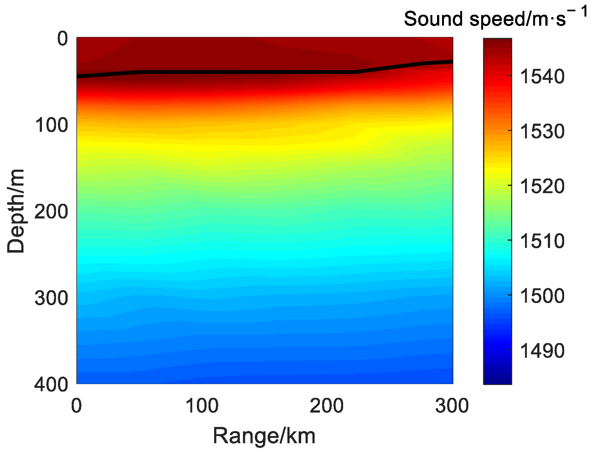
For the simulation, we considered a sea depth of 4500 m. The sound speed profile at a range of 0 km satisfied the Munk sound speed profile given by Equation (24). The Gaussian eddy parameters were set as follows: intensity of cyclonic eddy of $-30 m/s$, semi-major axis of 40 km, semi-minor axis of 400 m, eddy center $r_0=110 \mathrm{km}$, and $z_0=0 \mathrm{m}$. The sedimentary layer was considered as a fluid with a constant sound speed of 1650 m/s and density of $1.6 g/c{m}^3$. The acoustic absorption coefficient of the sedimentary layer was $0.5 dB/\lambda$.

Figure 5 shows the sound speed profile for the first 400 m. The source depth was 200 m, and the receiver depth was 3500 m. Thus, the receiver depth was below the conjugate depth of the sound source.

As for the linear variation in sound speed, the transmission loss in the range-independent and range-dependent environments was calculated using the normal and coupled normal modes, respectively. For the range-dependent environment, adiabatic approximation was used. The refracted and surface-reflected modes were selected in the simulation to calculate the transmission loss. The obtained transmission losses are shown in Figure 6.

To calculate the position of the convergence zone in a range-dependent environment with a Gaussian eddy using Equation (23), the modal strength of the normal modes of each order must be calculated. The corresponding results are shown in Figure 7. The modal strength of the lower mode is 0, and only the part with the larger amplitude is shown in the figure.

Figure 7 shows that the strongest modal intensity at receiver depth is achieved at mode 168. Computationally, the spread in mode $\Delta n$ is defined by two successive minima in the figure (i.e., $\Delta n=10$).

Table 2. Positions of convergence zones obtained using proposed formulation and coupled normal mode.

m	${\mathit{r}}_{\mathit{r}\mathit{i}}$/km	${\mathit{r}}_{\mathit{r}\mathit{d}}$/km	${\mathit{r}}_{\mathit{e}\mathit{q}}$/km
1	76.6	76.4	76.4
2	134.5	131.4	131.1
3	192.0	187.2	186.7
4	248.5	243.4	242.5
5	305.0	299.7	298.3
6	361.5	355.9	354.1
7	417.9	412.0	409.9

lists the positions of the convergence zones calculated according to Equation (23) and the coupled normal mode.

The columns of Table 2 have the same meanings as those of Table 1 but considering Equation (23) for column $r_{eq}$.

For the first convergence zone, Equation (23) agrees with the coupled normal mode theory. For other zones, there is an error between the two results, mainly because the skip distance is smaller than the numerical calculation. When considering the range of 400 km, an appropriate $\Delta n$ value is 14 for the position of the convergence zone to be 410.5 km. However, the error is only about 0.5% between the result of Equation (23) and the coupled normal mode in the seventh convergence zone, indicating that Equation (23) can be used to accurately calculate the position of the convergence zone in a range-dependent environment with a Gaussian eddy.

4. Experiments

4.1. Experimental Setup and Data Processing

In the summer of 2014, a deep-sea long-range sound propagation experiment was conducted in the South China Sea. An experimental diagram is shown in Figure 8. A hydrophone was placed at a depth of 3146 m, and the explosions at a depth of 200 m was selected as the sound source.

Figure 9 shows the sea depth measured in the experiment, which was approximately 4300 m, within 450 km of the entire experimental range. Figure 10 shows the sound speed profile at the hydrophone position measured by a conductivity, temperature, depth (CTD) sensor. The CTD is placed at the bottom of the submersible buoy. With the deployment and recovery of the submersible buoy, the sound speed profile of the whole depth can be obtained. The axis of the sound channel was approximately 1000 m. Figure 9 shows that the seabed in the first 300 km is flat, and there are three seamounts in 300–450 km. To ignore the impact of sea depth changes on the convergence zone, the experimental data for the first 300 km were selected for analysis.

To study the influence of sound speed variation, data represented by the hybrid coordinate ocean model (HYCOM) were used to obtain the sound speed profile in different ranges. The HYCOM data included temperature, salinity, density, and other parameters. Shaji et al. [24] showed that HYCOM data can be used to simulate a real environment. The precision of the HYCOM data selected for this study was 1/12°. By obtaining the temperature and salinity data from the experimental area and using Wood’s empirical formula for sound speed, we obtain the following variation in sound speed:

$$c=1450+4.206\times T-0.036\times T^2+1.137\times (S-35)+0.0175\times D,$$

(25)

where $c$ is the sound speed, $T$ is the temperature, $S$ is the salinity, and $D$ is the depth.

The sound speed profile over the first 400 m of depth obtained from the HYCOM data is shown in Figure 11, where the solid black line represents the depth of the maximum sound speed in the mixed layer. The variation in sound speed is mainly concentrated at a depth above 200 m, and the depth of the maximum sound speed in the mixed layer changes slightly with range. To further analyze the characteristics of the surface sound speed in the experimental area, the corresponding parameters were calculated for the environment within 200 m.

Figure 12 shows the average sound speed, salinity, temperature, refractive index of sound speed, sound speed gradient, and root-mean-square error (RMSE) of the sound speed for depths above 200 m. In each graph, the circle indicates the depth of the maximum sound speed in the mixed layer, and the asterisk represents the depth of the maximum sound speed gradient. The salinity, temperature, sound speed gradient, and RMSE of the sound speed show negligible changes above the depth of the maximum sound speed, and all the parameters have obvious changes from the depth of the maximum sound speed. Through Figure 12a–c, it is found that temperature is the main influencing factor of sound speed. At the depth of maximum sound speed gradient, the RMSE of the sound speed also reaches its maximum. Below this depth, the RMSE of sound speed decreases again. Figure 12 shows that the depth variation function can be described by the RMSE of sound speed, namely, $w\left(z\right)=c_{rmse}/\max \left(c_{rmse}\right)$ in Equation (16), where $c_{rmse}$ is the RMSE of sound speed.

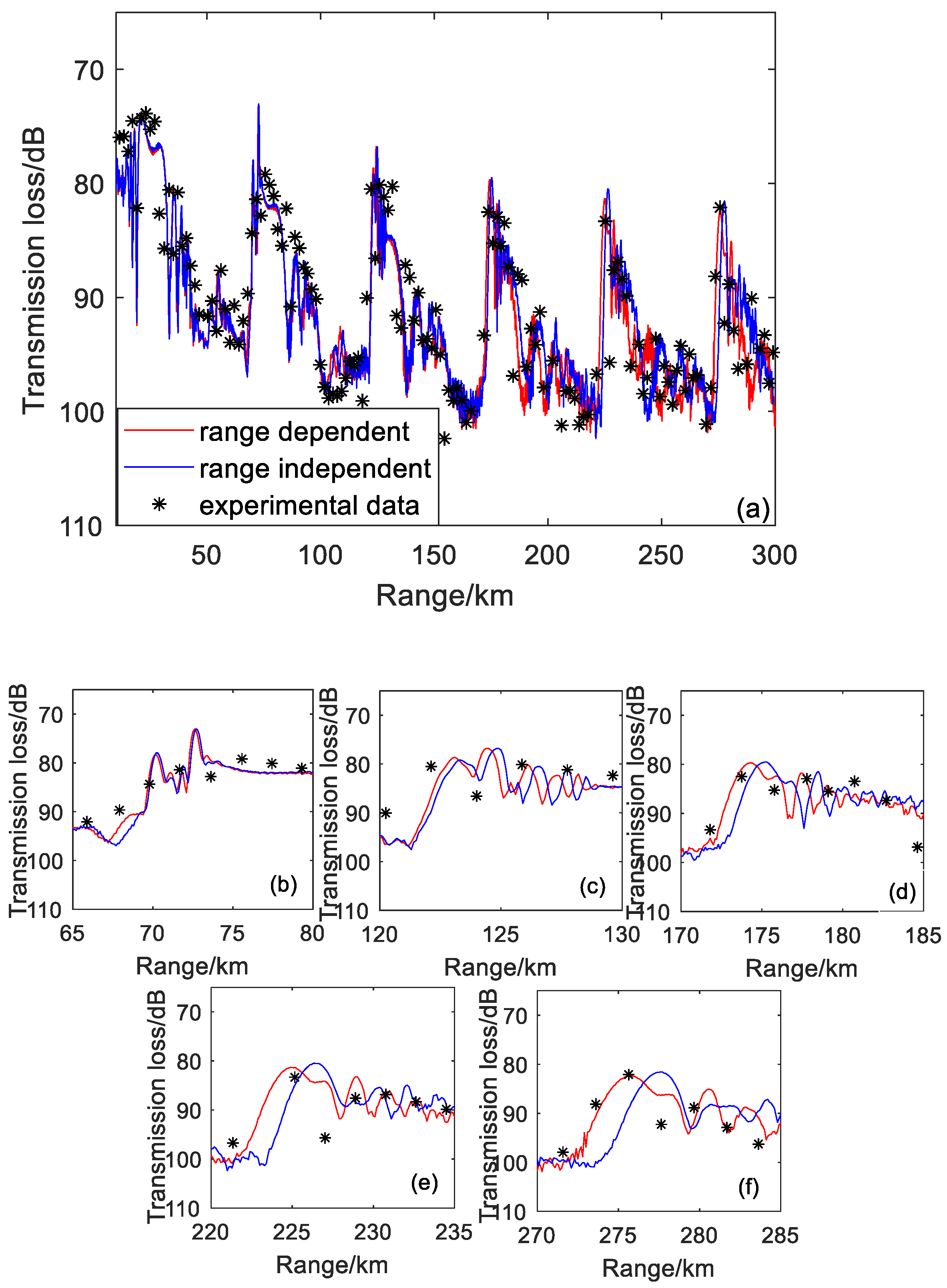
4.2. Experimental Results and Analysis

The sound source used in the experiment was an explosion located at a depth of 200 m. When calculating the transmission loss curve of the sound pressure field, the broadband explosion source is usually filtered in a one-third octave with a certain center frequency, and then the filtered signal is processed. We filtered the received signal with a one-third octave of the central frequency of 200 Hz, and the experimental transmission loss was calculated as

$$\mathrm{TL}\left(f_0|(r,z)\right)=\mathrm{SL}\left(f_0\right)-\left(10\lg \left[E\left(f_0\right)\right]-M_v-{\beta }_m\right),$$

(26)

where $\mathrm{SL}\left(f_0\right)$ is the source level of the explosion sound (199.8 dB in this experiment), $E\left(f_0\right)$ is the average energy within the signal bandwidth, $M_v$ is the sensitivity of the hydrophone (−185 dB), and ${\beta }_m$ is the amplification factor of the receiver (30 dB).

Figure 13 shows the transmission loss calculated from the experimental data and using normal mode theory. The asterisks indicate the results from experimental data, while the blue curve indicates the results of the range-independent environment, that is, the result calculated from the sound speed profile in Figure 10, and the red curve indicates the results of the range-dependent environment, that is, the result calculated from the sound speed profile in Figure 11. The change in sound speed profile is small within the first 150 km, and the position offset of the convergence zone caused by the sound speed variation is also small. After 150 km, the change in sound speed increases, and the position offset of the convergence zone also increases. Figure 13b–f show the transmission loss curves of the five convergence zones. The simulated transmission loss curve is more consistent with the experimental data when considering the sound speed variation.

We used Equation (20) to calculate the position of the convergence zone under sound speed variations. The sound source was located at 200 m, and the receiver depth was 3146 m, being below the reciprocal depth of the sound source. The modal strength of the normal modes, for which the phase speed is smaller than the bottom sound speed, is shown in Figure 14. The modal strength of the lower mode is 0, and only the part with larger amplitude is shown in the figure.

Figure 14 shows that mode 170 yields the strongest modal intensity at the receiver depth. Computationally, the spread in mode $\Delta n$ is defined by two successive minima in the figure (i.e., $\Delta n=17$), and the WKB approximation (Equation (4)) is considered. From the coupled normal mode, the horizontal wavenumber of mode 170 is 0.9297. Substituting this value into expression ${\kappa }_n\left(z\right)$ and using Equation (4), we obtain 7.8 × 10⁻⁴, being much less than 1 as required. Therefore, the refraction index is a slowly varying function of depth at this frequency. Equation (20) can be used to calculate the position of the convergence zone. The sound speed variation is calculated in segments with varying intensity parameter $\sigma$, such that $\delta c\left(z,r\right)$ is closer to the real sound speed profile. By substituting all the parameters into Equation (20), the position of the convergence zone is obtained.

Table 3. Positions of convergence zones obtained using proposed formulation and coupled normal mode on experimental data.

m	${\mathit{r}}_{\mathit{r}\mathit{i}}$/km	${\mathit{r}}_{\mathit{r}\mathit{d}}$/km	${\mathit{r}}_{\mathit{e}\mathit{x}}$/km	${\mathit{r}}_{\mathit{e}\mathit{q}}$/km
1	72.7	72.6	73.6	72.6
2	124.9	124.4	122.1	124.3
3	175.2	174.3	173.7	173.8
4	226.4	224.9	225.2	224.3
5	277.6	275.8	275.6	274.9

lists the results obtained from our derived formula and coupled normal mode. The position of the convergence zone obtained in the experiment is listed in the fourth column.

Equation (20) suitably provides the position of the convergence zone for a range-dependent sound speed profile. After the five convergence zones, there is a small difference of 0.9 km between the coupled normal mode and proposed formulation. The positions of the convergence zones obtained from the range-dependent and range-independent environments listed in Table 3 show that more convergence zones cause an increasing position offset owing to the sound speed variation. Because the variation in sound speed after 150 km accelerates, the absolute value of $\sigma$ increases. Thus, according to Equation (20), the position offset of the convergence zone increases.

Figure 15 shows the transmission losses in range-dependent and range-independent environments for sound source and receiver depths of 200 m. The transmission loss curve is basically the same in both cases, and the position and gain of the convergence zone are equal because the sound speed variation does not change considerably before 150 km. After 150 km, owing to the increasing sound speed variation, the transmission loss curve begins to exhibit differences, and the position and gain of the convergence zone change between the environments. In Figure 15, the fifth convergence zone is enlarged locally. Through the transmission loss curve, a position offset of 2.4 km occurs at the fifth convergence zone owing to the sound speed variation. Compared with the transmission loss curve in Figure 13 and enlarged view, the convergence zone is shifted by approximately 1.8 km owing to the sound speed variation at a receiver depth of 3146 m. For the sound source below the mixed layer, the influences of the sound speed variation with range on the convergence zone near the sea surface and the convergence zone for large-depth reception are similar, and the influence on the convergence zone for large-depth reception is smaller.

Figure 16 shows the results for a source depth of 100 m in the mixed layer. The receiver depths are 100 m and 3800 m, which is the reciprocal of 100 m. Before 150 km, given the small sound speed variation, the position and gain of the two types of convergence zones show negligible changes. When the sound speed variation changes notably after 150 km, it influences the position of the convergence zone. As the sound speed gradually decreases with range, the convergence zone shifts to the sound source, and the convergence zone near the sea surface is more affected than the convergence zone for large-depth reception. In this environment, the sound speed variation causes the convergence zone near the sea surface at the fifth convergence zone to shift by approximately 5 km, while the convergence zone for large depth reception only shifts by approximately 1 km.

Comparing Figure 13, Figure 15 and Figure 16, the variation in sound speed has a greater influence on the convergence zone when the source is at the mixed layer than when the source is below it. According to Equation (20), the upper and lower limits of the integral of $L_n$ in the molecule are related to the depth of the sound source, and the integral term contains depth function $w\left(z\right)$. When the sound source is located at the mixed layer, $w\left(z\right)$ is large, and the offset of the convergence zone distance increases. Comparing Figure 13 and Figure 16b, as the receiver depth increases, the influence of the sound speed variation on the position of the convergence zone for large-depth reception decreases.

5. Discussion

The results of the experimental data show that the formula derived in this paper can accurately predict the position of the convergence zone when the sound speed varys linearly. As for the ellipsoidal Gaussian eddy case, the simulation results verify the correctness of the formula. The position of the convergence zone in other mesoscale phenomena cases may also be derived as long as the specific $\delta c\left(z,r\right)$ can be expressed. However, further research is still needed for other cases of stochastic sound speed variation. In addition, for real world problems, the roughness of the sea surface needs to be incorporated into the stochastic part of the problem. Simulation and experimental data reveal that the convergence zone for large-depth reception has a good convergence gain, and it is less affected by the sound speed variation. Accurate prediction of the position of the convergence zone will play a key role in ocean acoustic tomography.

6. Conclusions

Based on the WKB approximation, we derived the position formulae of the convergence zone in a range-dependent environment with sound speed profiles varying in linear and ellipsoidal Gaussian eddy cases. The formulae obtained under the two profiles were simulated. By comparing the calculation results obtained from the coupled normal mode and derived formula, we verified the accuracy of the formula of the convergence zone position under a range-dependent sound speed profile. In addition, the derived formula under linear variation was verified using experimental data. The experimental data and convergence zone position simulated by the coupled normal mode were compared to further verify the correctness of the derived formula.

A simulation was carried out based on experimental data, and the influence of the sound speed variation on the position of the convergence zone was analyzed when the sound source was located at and below the mixed layer. We can draw the following conclusions: (1) When the sound source is located below the mixed layer, the sound speed variation reduces the offset in the position of the convergence zone, but the offset near the sea surface is larger than that of the convergence zone for large-depth reception. In the fifth convergence zone, the offset for the zone near the sea surface is approximately 2.4 km, and the position offset for large-depth reception is approximately 1.8 km. (2) When the sound source is located at the mixed layer, the influence of sound speed variation on the position of the convergence zone near the sea surface is substantially increased. However, the influence on the position of the convergence zone for large-depth reception decreases. In the fifth convergence zone, the position offset near the sea surface is approximately 5 km, and the offset for large-depth reception is approximately 1 km. Through simulation and experimental data, the convergence zone for large-depth reception also has a good convergence gain, increasing the applicability of this type of convergence zone. When considering long-range target detection, the convergence zone for large-depth reception is more appropriate than that near the sea surface because the former is less affected by sound speed variations.

References

1. Urick, R.J. Principle of Underwater Sound; McGraw-Hill: New York, NY, USA, 1983; pp. 79–162. [Google Scholar]
2. Woezel, J.L.; Ewing, M.; Pekeris, C.L. Explosion Sounds in Shallow Water. Geol. Soc. Am. Mem. 1948, 27, 1–62. [Google Scholar] [CrossRef]
3. Brekhovskikh, L.M. Propagation of acoustic and infrared waves in natural waveguides over long distances. Sov. Phys. Usp. 1960, 3, 159–166. [Google Scholar] [CrossRef]
4. Urick, R.J. Caustics and Convergence Zones in Deep-Water Sound Transmission. J. Acoust. Soc. Am. 1965, 38, 348–358. [Google Scholar] [CrossRef]
5. Schulkin, M. Surface-Coupled Losses in Surface Sound Channels. J. Acoust. Soc. Am. 1968, 44, 1152–1154. [Google Scholar] [CrossRef]
6. Bongiovanni, K.P.; Siegmann, W.L.; Ko, D.S. Convergence zone feature dependence on ocean temperature structure. J. Acoust. Soc. Am. 1996, 100, 3033–3041. [Google Scholar] [CrossRef]
7. Zhang, R.H. Normal mode sound field in shallow sea surface channel. Acta Phys. Sin. 1975, 24, 200–209. [Google Scholar] [CrossRef]
8. Wang, L.; Wang, K.P. Varieties of Sound Propagating in Convergence Zone Caused by Sound Spring Layer. Mar. Geod. Cartogr. 2014, 34, 40–42. [Google Scholar] [CrossRef]
9. Chen, C.; Yan, F.G.; Jin, T.; Zhou, Z.Q. Investigating acoustic propagation in the Sonic Duct related with subtropical mode water in Northwestern Pacific Ocean. Appl. Acoust. 2020, 169, 107478. [Google Scholar] [CrossRef]
10. Yang, F.; Wang, H.; Gao, W.D.; Meng, X.S. Zoning of sound speed profile types and characteristics of convergence zone in the deep North Atlantic Ocean. Mar. Forecast. 2021, 38, 103–110. [Google Scholar] [CrossRef]
11. Bi, S.Z.; Peng, Z.H. Effect of earth curvature on long range sound propagation. Acta Phys. Sin. 2021, 70, 114303. [Google Scholar] [CrossRef]
12. Henrick, R.F.; Siegmann, W.L. General analysis of ocean eddy effects for sound transmission applications. J. Acoust. Soc. Am. 1977, 62, 860–870. [Google Scholar] [CrossRef]
13. Rudnick, D.L.; Munk, W. Scattering from the mixed layer base into the sound shadow. J. Acoust. Soc. Am. 2006, 120, 2580–2594. [Google Scholar] [CrossRef]
14. Colosi, J.A.; Rudnick, D.L. Observations of upper ocean sound-speed structures in the North Pacific and their effects on long-range acoustic propagation at low and mid-frequencies. J. Acoust. Soc. Am. 2020, 148, 2040–2060. [Google Scholar] [CrossRef] [PubMed]
15. Li, J.X.; Zhang, R. Ocean mesoscale eddy modeling and its application in studying the effect on underwater acoustic propagation. Mar. Sci. Bull. 2011, 30, 37–46. [Google Scholar] [CrossRef]
16. Colosi, J.A.; William, Z.L. Sensitivity of mixed layer duct propagation to deterministic ocean features. J. Acoust. Soc. Am. 2021, 149, 1969–1978. [Google Scholar] [CrossRef]
17. White, A.W.; Henyey, F.S. Internal tides and deep diel fades in acoustic intensity. J. Acoust. Soc. Am. 2016, 140, 3952–3962. [Google Scholar] [CrossRef]
18. Zhang, L.; Liu, D. Deep-sea acoustic field effect under mesoscale eddy conditions. Mar. Sci. 2020, 44, 66–73. [Google Scholar] [CrossRef]
19. Piao, S.C.; Li, Z.Y. Lower turning point convergence zone in deep water with an incomplete channel. Acta Phys. Sin. 2021, 70, 024301. [Google Scholar] [CrossRef]
20. Wu, S.L.; Li, Z.L.; Qin, J.X.; Wang, M.Y. Influence of tropical dipole in the East Indian Ocean on acoustic convergence region. Acta Phys. Sin. 2022, 71, 134301. [Google Scholar] [CrossRef]
21. Chandrayadula, T.K.; Periyasamy, S.; Colosi, J.A. Observations of low-frequency, long-range acoustic propagation in the Philippine Sea and comparisons with mode transport theory. J. Acoust. Soc. Am. 2020, 147, 877–897. [Google Scholar] [CrossRef]
22. Tindle, C.T.; Guthrie, K.M. Rays as interfering modes in underwater acoustics. J. Sound Vib. 1974, 34, 291–295. [Google Scholar] [CrossRef]
23. Beilis, A. Convergence zone positions via ray mode theory. J. Acoust. Soc. Am. 1983, 74, 171–180. [Google Scholar] [CrossRef]
24. Shaji, C.; Wang, C.; Halliwell, G.R. Simulation of tropical Pacific and Atlantic Oceans using a HYbrid Coordinate Ocean Model. Ocean Model. 2005, 9, 253–282. [Google Scholar] [CrossRef]
Figure 1. Sound speed profile with linear variation.
Remotesensing 14 06314 g001
Figure 2. Depth variable function in linear variation case.
Remotesensing 14 06314 g002
Figure 3. Transmission losses in range-independent and range-dependent environments for linearly varying sound speed.
Remotesensing 14 06314 g003
Figure 4. Mode amplitudes for refracted and surface-reflected modes considering linearly varying sound speed.
Remotesensing 14 06314 g004
Figure 5. Sound speed profile of Gaussian eddy.
Remotesensing 14 06314 g005
Figure 6. Transmission losses in range-independent and range-dependent environments for ellipsoidal Gaussian eddy case.
Remotesensing 14 06314 g006
Figure 7. Mode amplitudes for refracted and surface-reflected modes considering ellipsoidal Gaussian eddy case.
Remotesensing 14 06314 g007
Figure 8. Diagram of experimental setup for data collection. The sound source is represented as a star mark.
Remotesensing 14 06314 g008
Figure 9. Bathymetry along experimental path.
Remotesensing 14 06314 g009
Figure 10. Sound speed profile at hydrophone position.
Remotesensing 14 06314 g010
Figure 11. Sound speed profile obtained from HYCOM data.
Remotesensing 14 06314 g011
Figure 12. Parameters obtained for depths above 200 m. (a) Average sound speed, (b) salinity, (c) temperature, (d) refractive index of sound speed, (e) sound speed gradient, and (f) RMSE of sound speed. The circle indicates the depth of the maximum sound speed in the mixed layer, and the asterisk represents the depth of the maximum sound speed gradient.
Remotesensing 14 06314 g012
Figure 13. Transmission loss obtained from experiment and simulation. Results from (a) complete path and from (bf) first to fifth convergence zones. In each graph, red line is the result of range dependent case. Blue line is the result of range independent case. The asterisk is the result of experimental data.
Remotesensing 14 06314 g013
Figure 14. Mode amplitudes for refracted and surface-reflected modes obtained from experimental data.
Remotesensing 14 06314 g014
Figure 15. Transmission loss obtained from range-independent and range-dependent sound speed profiles with source and receiver depths of 200 m.
Remotesensing 14 06314 g015
Figure 16. Transmission loss obtained from range-independent and range-dependent sound speed profiles at source depth of 100 m and receiver depths of (a) 100 and (b) 3800 m.
Remotesensing 14 06314 g016