Tree Species Classification from Airborne Hyperspectral Images Using Spatial–Spectral Network

Abstract

Tree species identification is a critical component of forest resource monitoring, and timely and accurate acquisition of tree species information is the basis for sustainable forest management and resource assessment. Airborne hyperspectral images have rich spectral and spatial information and can detect subtle differences among tree species. To fully utilize the advantages of hyperspectral images, we propose a double-branch spatial–spectral joint network based on the SimAM attention mechanism for tree species classification. This method achieved high classification accuracy on three tree species datasets (93.31% OA value obtained in the TEF dataset, 95.7% in the Tiegang Reservoir dataset, and 98.82% in the Xiongan New Area dataset). The network consists of three parts: spectral branch, spatial branch, and feature fusion, and both branches make full use of the spatial–spectral information of pixels to avoid the loss of information. In addition, the SimAM attention mechanism is added to the feature fusion part of the network to refine the features to extract more critical features for high-precision tree species classification. To validate the robustness of the proposed method, we compared this method with other advanced classification methods through a series of experiments. The results show that: (1) Compared with traditional machine learning methods (SVM, RF) and other state-of-the-art deep learning methods, the proposed method achieved the highest classification accuracy in all three tree datasets. (2) Combining spatial and spectral information and incorporating the SimAM attention mechanism into the network can improve the classification accuracy of tree species, and the classification performance of the double-branch network is better than that of the single-branch network. (3) The proposed method obtains the highest accuracy under different training sample proportions, and does not change significantly with different training sample proportions, which are stable. This study demonstrates that high-precision tree species classification can be achieved using airborne hyperspectral images and the methods proposed in this study, which have great potential in investigating and monitoring forest resources.

1. Introduction

Forests are the mainstay of terrestrial ecosystems and are essential in maintaining ecological security and balance [1]. Conducting forest resource surveys and monitoring is important for formulating forestry guidelines and policies, protecting and utilizing planned forests, and constructing a sound ecological environment [2]. Among these, tree species identification is one of the basic and key components of forest resources monitoring, which plays a vital role in forest fire prevention [3], the monitoring of forest pests and diseases [4], the extraction of forest change information [5], and the protection of biodiversity [6]. Traditional tree species identification mainly relies on manual field surveys to identify tree species based on the external morphology of trees. Although this method has high accuracy, it has low accessibility, involves a difficult investigation, and involves high danger for plots without traffic conditions [7]. Secondly, field survey is costly and time-consuming, which makes it challenging to identify large-scale tree species in a short time.

The rapid development of remote sensing technology makes up for the deficiency of manual survey methods, which can obtain large-area image data without touching trees and realize the classification and identification of tree species in large regional scale areas without causing damage to the forest ecological environment. In particular, the hyperspectral sensor can simultaneously image the target region in tens to hundreds of continuous and subdivided spectral bands, obtaining the spatial information of the surface image as well as its spectral information, achieving the combination of spectra and image. Compared with RGB and multispectral images, hyperspectral images have rich spectral information and can detect subtle differences in the spectra of different vegetation, which has significant advantages in forest tree species classification.

In recent years, deep learning methods based on neural network have become popular with the development of computer hardware and algorithms. As an emerging research direction in the field of machine learning, it utilizes deep neural network structures that can automatically learn high-level abstract features and combine these features layer by layer to achieve efficient and accurate data classification and prediction [8,9]. Compared with traditional machine learning methods, deep learning has more robust self-adaptive and generalization capabilities, can better handle large-scale complex data, and has achieved great success in computer vision, natural language processing, speech recognition, and other fields. In the field of remote sensing, deep learning technology has attracted extensive attention from scholars, and many experts have utilized deep learning methods for tree species classification and achieved good classification results [10,11,12]. Among them, the convolutional neural network (CNN) has achieved remarkable results in computer vision, such as image classification [13], object detection [14], and semantic segmentation [15]. Due to its powerful feature extraction capability, the convolutional neural network has become the most commonly used neural network in hyperspectral tree species classification [16,17,18]. The hyperspectral image classification methods based on CNN can be mainly divided into three classes:

• Classification methods based on spectral features [19,20]. This method utilizes 1D-CNN to extract features from the raw spectral information of pixels to complete classification. Xi et al. [21] applied a 1D-CNN to tree species classification in OHS-1 hyperspectral images, and the results showed that the accuracy obtained using a 1D-CNN (85.04%) was better than that of the Random Forest classification model (80.61%). However, the 1D-CNN only considered the spectral information of the samples and not their spatial information.
• Classification methods based on spatial features [22,23]. This method first performs feature dimensionality reduction on hyperspectral images and then extracts spatial information in a neighborhood centered on the pixel to be classified, using a 2D-CNN to complete classification. Fricker et al. [24] performed PCA dimensionality reduction on hyperspectral data, used a 2D-CNN to extract spatial features from the data after dimensionality reduction, and classified seven dominant species and dead trees in a mixed coniferous forest, achieving a classification accuracy of 87%. Although the 2D-CNN utilizes the spatial information of pixels, it loses the original spectral information in the dimensionality reduction process.
• Classification methods based on spatial–spectral features association. One way is to use a 3D-CNN to simultaneously extract spectral and spatial features of pixels [25,26]. Zhang et al. [27] proposed an improved 3D convolutional neural network for tree species classification, which uses the raw data of airborne hyperspectral images as input without dimensionality reduction or feature selection and can extract spectral and spatial features simultaneously, resulting in a tree species classification accuracy of 93.14%. However, this method only uses the 3D convolutional structure, which can easily lead to overfitting when the number of network parameters is large. Another way is to use different networks to extract spectral and spatial features separately, and then combine the two features to complete classification [28,29,30]. For example, Liang et al. [31] proposed a spectral–spatial paralleled convolutional neural network to classify the forest tree species in the UAV HSI. The experimental results showed that the SSPCNN produced competitive performance compared with other methods. However, the network structure is relatively simple, and the classification effect is not good in the context of complex forests.

In short, methods based on spectral or spatial features may lose certain information and fail to take full advantage of hyperspectral images. Hyperspectral images contain both spatial and rich spectral information, so classification methods based on spatial–spectral feature association are more in line with hyperspectral characteristics. Compared with a 3D-CNN, the double-branch network can design different forms of spectral and spatial networks to extract features, which has more flexibility and a strong advantage in hyperspectral tree species classification. In tree species classification, different spectral features and spatial features have different abilities to distinguish tree species, and the neural network should focus on the features that contribute significantly to the classification results. Therefore, the accuracy of tree species classification can be improved by introducing an attention mechanism to make the network focus on important features and suppress unimportant features.

In summary, tree species identification is essential for forest inventory, and remote sensing technology has strong advantages in large-scale tree species identification. Since airborne hyperspectral images have rich spectral and spatial information, which can detect subtle differences between different tree species, we used hyperspectral images as the data source. However, the classification methods based on spectral features do not consider the spatial information of hyperspectral images, and the classification methods based on spatial features will cause the loss of spectral information in the process of data dimensionality reduction. In addition, the neural network should focus on features that contribute significantly to classification. In order to fully utilize the spatial–spectral information of hyperspectral images, we design a double-branch network, i.e., a spectral branch and a spatial branch. In the spectral branch, we utilize a 3D-CNN to extract spectral features of pixels instead of a 1D-CNN, which avoids the loss of spatial information. In the spatial branch, we use muti-scale convolution and a 2D-CNN to extract spatial features of pixels. It is worth noting that we do not reduce the dimensionality of the original data, but input all the spectral bands into the spatial branch, which avoids the loss of spectral information in the process of dimensionality reduction. In both branches, we design corresponding residual structure blocks to extract features better. To further utilize the spatial–spectral information, we fuse the features obtained from the two branches through a concatenation operation to obtain spatial–spectral features. In addition, the neural network should focus on features that contribute significantly to classification. So, we introduce the SimAM (Simple Parameter-Free Attention Module) mechanism into the network, which is a parameter-free attention mechanism that can make the network focus on important features without increasing the number of parameters of the network. Finally, the fully connected layer is utilized to complete tree species classification.

Our main contributions can be summarized as follows:

1.

To fully utilize the advantages of the airborne hyperspectral images, we propose a double-branch spatial–spectral joint network based on the SimAM attention mechanism for tree species classification. The network consists of three parts: spectral branch, spatial branch, and feature fusion. The spatial–spectral information of pixels is utilized in both spectral and spatial branches to extract features, and spatial and spectral features are merged in the feature fusion stage. Moreover, the SimAM attention mechanism is used to refine the features further to improve the classification accuracy.

2.

To verify the effectiveness of the proposed method, we conducted tree species classification experiments on three different tree species datasets, and the experimental results showed that the method proposed in this study performed the best and obtained the highest tree species classification accuracy compared to other classification methods. Furthermore, we further verified the importance of joint spatial–spectral information and the SimAM attention mechanism through ablation experiments. Finally, we analyzed the factors affecting the classification accuracy of tree species.

The rest of this article is organized as follows: Section 2 describes the related work. Section 3 describes the three tree species datasets used in this study and the proposed method in detail. Section 4 presents classification results. Section 5 discusses and analyzes the classification of tree species from different perspectives. Finally, the manuscript presents the conclusions and briefly describes the directions for future work.

2. Related Work

2.1. Tree Species Classification Based on Remote Sensing Technology

Recent advances in remote sensing technology hold much promise for the detailed mapping of the spatiotemporal distribution and characteristics of tree species over wide areas. Many researchers have successfully utilized remote sensing technology for tree species classification studies [32,33,34]. Park et al. [35] combined high-resolution RGB images (spatial resolution of 7 cm) acquired using UAV with machine learning algorithms to monitor trees and leaf phenology in Panama’s tropical forests. Grabska et al. [36] created nine different subsets of variables from multi-temporal Sentinel-2 data and environmental terrain data (elevation, slope, and slope direction) using a Random Forest-based variable importance selection algorithm (VSURF) and Recursive Feature Elimination (RFE). They classified the tree species using Random Forest, Support Vector Machine, and XGBoost algorithms, respectively. The results showed that the Support Vector Machine classifier outperforms the other two classifiers, obtaining the highest accuracy of 86.9%. Although RGB and multispectral remote sensing data have been widely used in tree species classification, the characteristics between some tree species (especially those of the same genus) are very similar, making it difficult to classify them finely with these two data sources.

2.2. Classification Methods Based on Hyperspectral Images

While RGB and multispectral data were reported to have potential for tree species mapping, the continuous spectral information contained in hyperspectral data seems even more suitable to differentiate tree species with similar spectral properties. In previous studies, tree species classification using hyperspectral data mainly adopted traditional machine learning methods [37,38,39], such as Support Vector Machine, Random Forest, BP neural network, etc. For example, Dalponte et al. [40] used hyperspectral data and three classifiers (SVM, RF, and Maximum Likelihood method) to evaluate the accuracy of boreal forest species classification at the pixel level and crown level, respectively. However, traditional machine learning methods need to process and transform the raw data and manually extract features with distinction, such as important bands, vegetation indices, and texture features. The performance results of the methods largely depend on whether the selected features are reasonable or not. However, feature selection often relies on experience and is somewhat blind. In addition, the selected feature type depends on the specific task and dataset, which needs to be decided according to the actual situation, resulting in poor generalization ability. Wei et al. [41] proposed a fine classification method based on multi-feature fusion and deep learning. In their research, the morphological profiles, GLCM texture and endmember abundance features were leveraged to exploit the spatial information of the hyperspectral imagery. Then, the spatial information was fused with the original spectral information to generate classification results by using the deep neural network with a conditional random field (DNN + CRF) model. Although this method can yield good classification results, the spatial features are manually extracted from the raw data, which consumes time.

2.3. Attention Mechanism

As is known to all, the importance of every spectral channel and the area of the input patch is different when the network extracts features. The attention mechanisms can focus on the most informative part and decrease the weight of other regions. Many researchers have introduced an attention mechanism into hyperspectral image classification. Ma et al. [42] introduced the Convolutional Block Attention Module (CBAM) into hyperspectral images classification and proposed a Double-Branch Multi-Attention mechanism network (DBMA) for HSI classification. The experimental results demonstrated the effectiveness of the attention mechanism in hyperspectral images classification. However, current attention mechanisms often use additional sub-networks to generate attention weights [43,44,45], increasing the number of parameters in the model. The hyperspectral images have a massive amount of data compared to other remote sensing data sources. Accordingly, the number of parameters in the network model is also huge. The parameter-free attention mechanism does not introduce additional parameters to the network in generating weights, which is more suitable for hyperspectral images classification.

3. Materials and Methodology

3.1. Dataset Introduction

To verify the robustness of the proposed method, we conducted tree species classification experiments on three different hyperspectral datasets. The three study areas are located in different spatial locations, and the datasets are acquired using various hyperspectral sensors, with different spatial resolutions and different tree species categories. Next, the three datasets are described in detail.

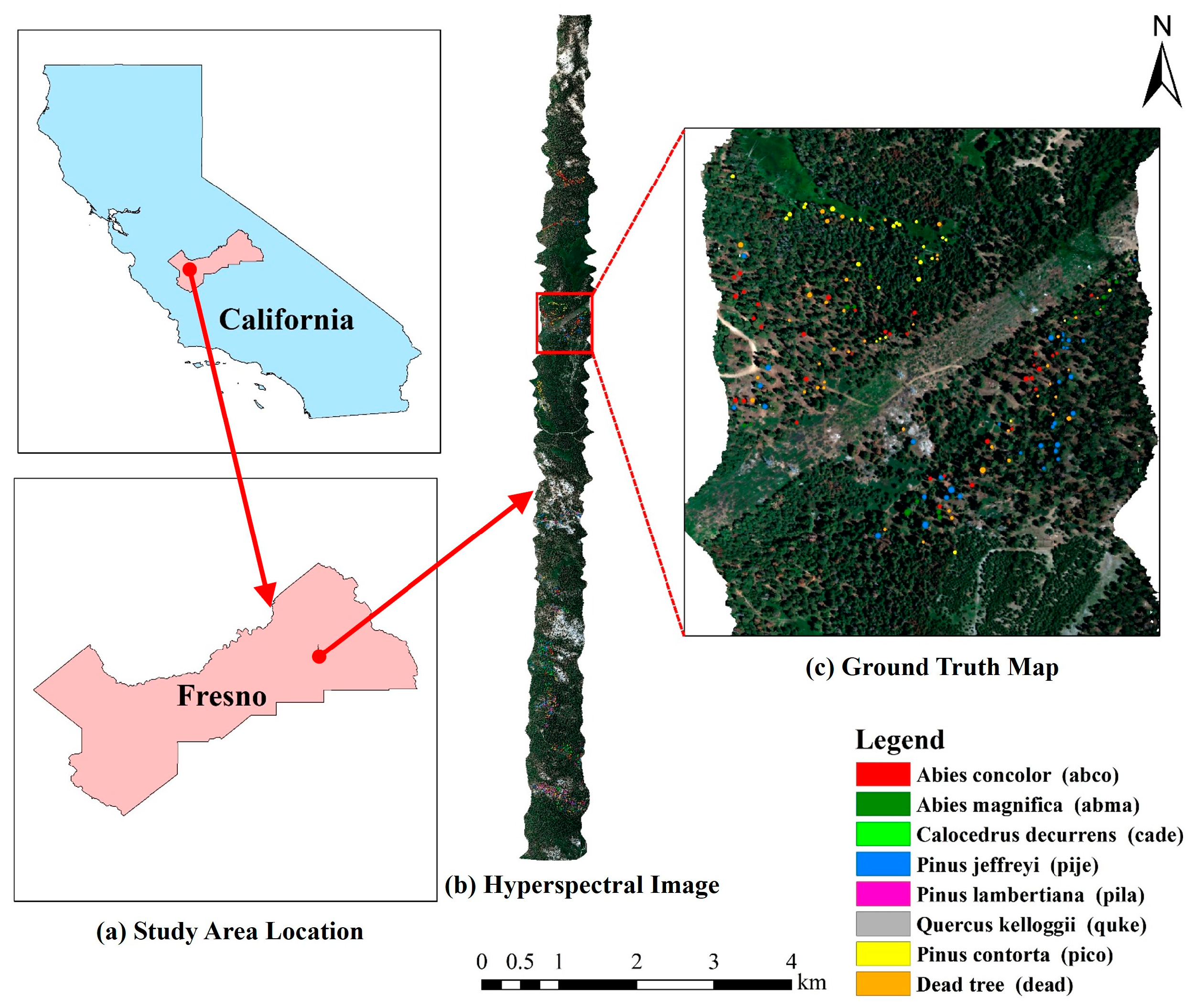
3.1.1. TEF Dataset

The Teakettle Experimental Forest (TEF) study area is located in northeastern Fresno, California, USA (36°59′51″N, 119°1′28″W), near the southern Sierra Nevada Mountains, as shown in Figure 1a. The TEF dataset was collected in 2017 by the National Ecological Observatory Network (NEON) using the airborne remote sensing platform AOP. A south-to-north flight strip, approximately 16 km long and 1 km wide, covering a portion of the Teakettle Experimental Forest, was used for this study. The hyperspectral sensor covers a wavelength range of 380–2510 nm with a spectral sampling interval of 5 nm, resulting in 426 bands. Data acquisition using the remote sensing platform occurred at an altitude of approximately 1000 m above the ground, resulting in an image spatial resolution of 1 m. After removing the empty band and the bands affected by water vapor absorption, the remaining 388 bands were used for experiments. The hyperspectral data was preprocessed by NEON at the time of dataset release, including radiometric calibration, geometric correction, atmospheric correction, and orthometric correction. Field data was provided by Geoffrey et al. [24], and includes seven dominant tree species and dead trees.

The dataset was divided using a stratified random sampling method in this study. Specifically, a fixed proportion of data from each category was selected as the training and test sets. To avoid the chance of random selection in the dataset production process, we adopted a 5-fold cross-validation method to obtain five datasets. In each experiment, five datasets were trained and tested, respectively, and the average value was taken as the final classification result. The specific number of training and test sets for each category in the TEF dataset is shown in

Table 1. The number of training samples and test samples in the TEF dataset.

Code	Scientific Name	Abbreviation	Train Samples	Test Samples
1	Abies concolor	abco	2323	593
2	Abies magnifica	abma	742	113
3	Calocedrus decurrens	cade	1452	403
4	Pinus jeffreyi	pije	3654	924
5	Pinus lambertiana	pila	2205	583
6	Quercus kelloggii	quke	96	14
7	Pinus contorta	pico	741	154
8	Dead tree	dead	2745	796
Total			13,958	3580

.

3.1.2. Tiegang Reservoir Dataset

The Tiegang Reservoir study area is located in the southeastern part of Baoan District, Shenzhen City, Guangdong Province, China (22°36′30″N, 113°54′30″E), as shown in Figure 2a. The image was collected using an independently integrated UAV hyperspectral system of the Chinese Academy of Surveying and Mapping. The hyperspectral sensor is a push-broom scanner that records 112 bands in the 400–1000 nm spectral range with a spectral resolution of 5 nm. The flight altitude was set to 100 m above ground level, resulting in an image spatial resolution of 0.1 m. We performed pre-processing operations such as outlier removal, radiometric calibration, geometric correction, atmospheric correction, and image mosaic on the raw image. The hyperspectral image is shown in Figure 2b. Field data was collected at the end of the flight process, and contained a total of seven tree species.

Because the spatial resolution of the Tiegang Reservoir dataset is 0.1 m, and the number of pixels is more compared to the TEF dataset, we did not use a 5-fold cross-validation method to produce the dataset; instead, the training set and the test set were divided according to the ratio of 1:1. The above operation was repeated five times, and its average value was calculated as the final classification result. The specific number of training and test sets for each category in the Tiegang reservoir dataset is shown in

Table 2. The number of training samples and test samples in the TieGang Reservoir dataset.

Code	Scientific Name	Abbreviation	Train Samples	Test Samples
1	Glyptostrobus pensilis	glpe	10,013	6581
2	Cinnamomum camphora	cica	53,577	49,912
3	Eucalyptus robusta Smith	euro	14006	7868
4	Ficus altissima	fial	1783	3990
5	Platycladus orientalis	plor	19,287	10,021
6	Ficus microcarpa	fimi	10,226	6997
7	Castanopsis hystrix	cahy	9627	14,518
Total			118,519	99,887

.

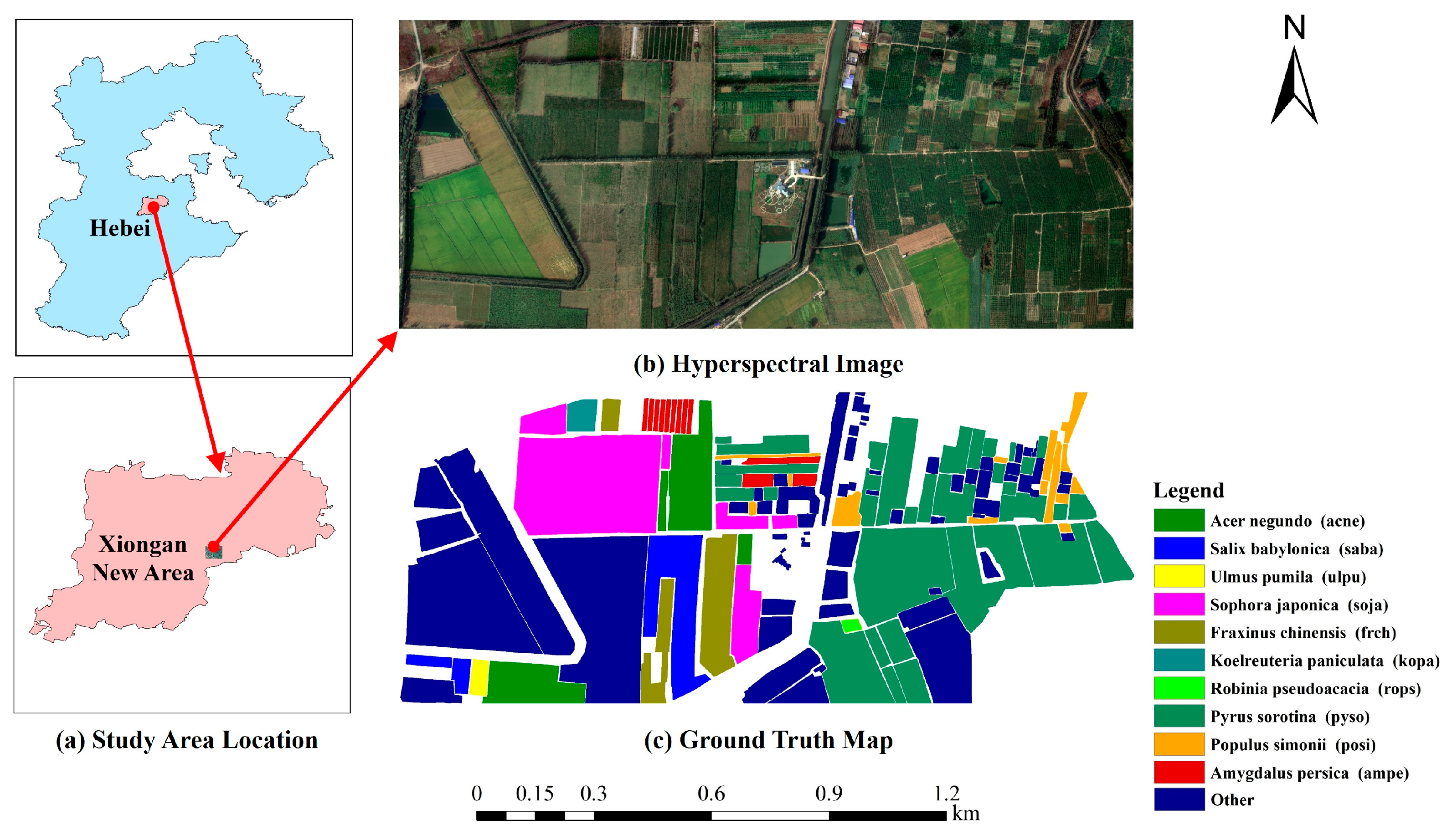
3.1.3. Xiongan New Area Dataset

The Xiongan New Area study area is located in the Matiwan Village, in the southeastern part of Xiongan New Area, Hebei Province, China (38°56′40″N, 116°3′57″E), as shown in Figure 3a. The hyperspectral image was collected in October 2017 by the Institute of Remote Sensing and Digital Earth and the Shanghai Institute of Technical Physics of the Chinese Academy of Sciences. The hyperspectral sensor covers a wavelength range of 390-1000 nm, with a spectral sampling interval of approximately 2.4 nm, resulting in 256 bands. The data was collected using the airborne remote sensing platform at about 2000 m from the ground, resulting in an image spatial resolution of 0.5 m. The image contains 3750 × 1580 pixels, as shown in Figure 3b. Through the field investigation of land cover types, 20 categories were annotated, as shown in Figure 3c, including many tree species, such as Pyrus sorotina, Acer negundo, Salix babylonica, etc.

The Xiongan New Area dataset differs from the other two datasets. All trees are artificial plantations, which are uniformly distributed, and the boundaries between different tree species are clear. Considering the difficulty and high cost of sample acquisition in practical remote sensing applications for forests, the tree species classification performance of the network was explored with limited training samples. Specifically, we randomly selected 0.5% of the data from each category as the training set and 5% of the data as the test set. The objects of the study were various typical broadleaf tree species in northern China, so the categories of non-tree objects were categorized as other. Similarly, the above operation was repeated five times to avoid the chance of random selection, resulting in five datasets. The five datasets were trained and tested in each experiment, and the average value was taken as the final classification result. The specific number of training and test sets for each category in the Xiongan New Area dataset is shown in

Table 3. The number of training samples and test samples in the Xiongan New Area dataset.

Code	Scientific Name	Abbreviation	Train Samples	Test Samples
1	Acer negundo	acne	1128	11282
2	Salix babylonica	saba	903	9038
3	Ulmus pumila	ulpu	76	767
4	Sophora japonica	soja	2377	23,779
5	Fraxinus chinensis	frch	846	8467
6	Koelreuteria paniculata	kopa	116	1165
7	Robinia pseudoacacia	rops	28	280
8	Pyrus sorotina	pyso	5132	51,325
9	Populus simonii	posi	455	4553
10	Amygdalus persica	ampe	327	3275
11	Other	other	6987	69,915
Total			18,375	183,846

.

3.2. Methodology

The hyperspectral image data $\mathit{X}\in {\mathbb{R}}^{H\times W\times B}$(where $H\times W$ and $B$ denote the spatial size of HSI and the number of spectral bands, respectively) are a three-dimensional structure, which contains spatial information and rich spectral information. To better classify HSI pixels ${\mathit{x}}_{\mathit{i}}\in {\mathbb{R}}^{1\times 1\times B}$ with spectral and spatial information, the HSI patch ${\mathit{X}}_{\mathit{i}}\in {\mathbb{R}}^{L\times L\times B}$ is cropped from $\mathit{X}$ and input into the neural network to extract spatial–spectral features. 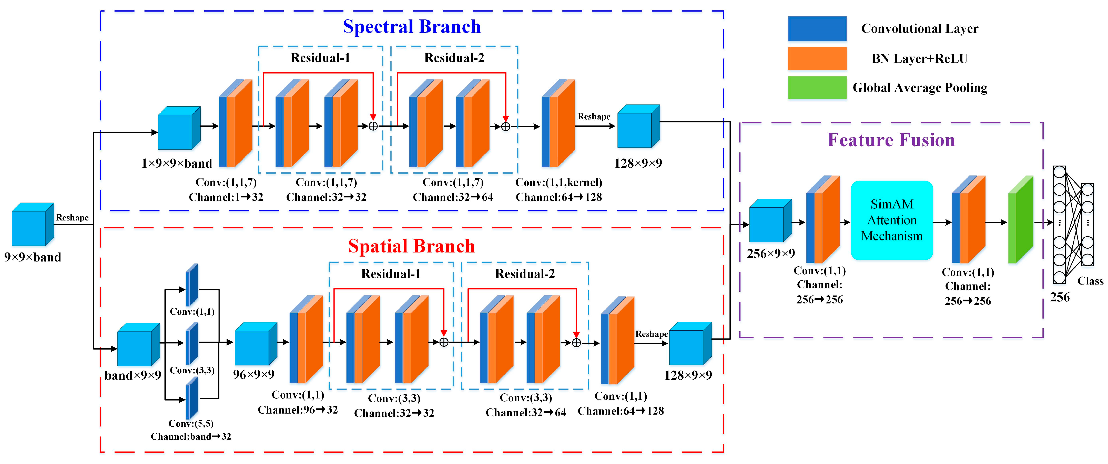Here, the center pixel of ${\mathit{X}}_{\mathit{i}}$ is ${\mathit{x}}_{\mathit{i}}$, and $L\times L$ is patch size, chosen in this study to be 9 × 9. Moreover, to fully utilize the advantages of hyperspectral images, we proposed a double-branch spatial–spectral joint network based on the SimAM attention mechanism for tree species classification. The network structure is shown in Figure 4, and consists of three parts: spectral branch, spatial branch, and feature fusion. Specifically, the spectral branch mainly uses a 3D-CNN to extract the spectral features of pixels. The spatial branch mainly uses a 2D-CNN to extract the spatial features of pixels. To make further use of the spatial–spectral information of hyperspectral data, we fuse the features extracted from the spectral branch with those extracted from the spatial branch, and introduce the SimAM attention mechanism in the fusion stage. By assigning different weights to each part of the feature map, important features are extracted, and unimportant features are suppressed, thus improving the classification accuracy of tree species.

3.2.1. Spectral Branch

When extracting the spectral features of pixels using a 1D-CNN, the spatial information of the data will be lost, while a 3D-CNN extracts the spectral features along with their spatial features, which can avoid the loss of spatial information. Therefore, in the spectral branch, we utilize a 3D-CNN to extract the spectral features of pixels. The 3D convolution operation is as in Equation (1):

$$v_{l,j}^{x,y,z}=f(\sum _m\sum _{h=0}^{H_l-1}\sum _{w=0}^{W_l-1}\sum _{r=0}^{R_l-1}{\omega }_{l,j,m}^{h,w,r}{v}_{\left(l-1\right),m}^{\left(x+h\right),\left(y+w\right),(z+r)}+b_{l,j})$$

(1)

where, $v_{l,j}^{x,y,z}$ is the value at position $(x,y,z)$ on the jth feature cube in the lth layer. $H_l$ and $W_l$ denote the height and width of the 3D convolution kernel in the spatial dimension, respectively, and $R_l$ denotes the 3D convolution kernel in the spectral dimension. ${\omega }_{l,j,m}^{h,w,r}$ is the weight parameter at position $(h,w,r)$ of the $j$th convolution kernel in the $l$th layer, and the convolution kernel is connected to the mth feature cube in the $(l-1)$th layer. $v_{\left(l-1\right),m}^{\left(x+h\right),\left(y+w\right),(z+r)}$ is the value at position $(x+h,y+w,z+r)$ on the $m$th feature cube in the $(l-1)$th layer. $b_{l,j}$ is the bias value. $f(·)$ is the activation function; we chose the ReLU activation function in this study.

The input data format for the spectral branch is (1, 9, 9, band), which contains all pixels within a neighborhood size of 9 × 9 centered on the pixel to be classified. First, we convolve the data using a 3D convolution kernel of size (1, 1, 7) to increase the number of channels to 32. After that, we design two spectral residual blocks to extract features further. The residual structure connects the convolutional layers through identity mapping, which promotes a better backpropagation of the gradient and helps to solve the problem of gradient vanishing and explosion [46]. Each spectral residual block consists of two 3D convolutional layers. Meanwhile, in order to speed up the training and convergence of the network and prevent model overfitting, we add a Batch Normalization (BN) layer after each convolutional layer of the network to improve the model performance. Finally, we utilize a 3D convolutional kernel of size (1, 1, kernel), where kernel denotes the number of bands remaining after a series of convolutions, to obtain a spectral feature map of size (128, 9, 9), denoted by $F_{spectral}$.

3.2.2. Spatial Branch

In the spatial branch, we utilize a 2D-CNN to extract the spatial features of hyperspectral images. A 2D-CNN mainly uses a 2D convolution kernel to perform convolution operations on 2D data. The value ${map}_{l,j}^{x,y}$ at position $(x,y)$ on the $j$th feature map in the $l$th layer is:

$${map}_{l,j}^{x,y}=f(\sum _m\sum _{h=0}^{H_l-1}\sum _{w=0}^{W_l-1}{\omega }_{l,j,m}^{h,w}{map}_{\left(l-1\right),m}^{\left(x+h\right),(y+w)}+b_{l,j})$$

(2)

where, $H_l$ and $W_l$ denote the height and width of the 2D convolution kernel, respectively. ${\omega }_{l,j,m}^{h,w}$ is the weight parameter at position $(h,w)$ of the $j$th convolution kernel in the $l$th layer, and the convolution kernel is connected to the $m$th feature map in the $(l-1)$th layer. ${map}_{\left(l-1\right),m}^{\left(x+h\right),(y+w)}$ is the value at position $(x+h,y+w)$ on the $m$th feature map in the $(l-1)$th layer. $b_{l,j}$ is the bias value. $f(·)$ is the activation function; similarly, we chose the ReLU activation function in the spatial branch.

In previous studies, when researchers extracted spatial features of hyperspectral images using a 2D-CNN, they first processed the raw data using a dimensionality reduction algorithm (e.g., PCA algorithm), and then used the neural network for classification. However, in the process of performing feature dimensionality reduction, the spectral information of the data will be lost. To avoid the loss of information, instead of performing dimensionality reduction on the data, we input all of the original spectral bands of the pixels into the network. Hence, the input data format of the spatial branch is (band, 9, 9). In the spatial branch, we first extract the multi-scale spatial features of the data using multi-scale convolution (the convolution kernels are 1 × 1, 3 × 3, and 5 × 5, respectively). The number of output channels is 32, and three sets of feature maps with sizes of (32, 9, 9) are obtained, respectively. Then, the three sets of features are combined to form a muti-scale feature map used as input to the subsequent convolutional layers, as shown in Equation (3).

$$F_{muti}=Concat(F_{1\times 1},F_{3\times 3},F_{5\times 5})$$

(3)

where, $F_{muti}$ denotes the muti-scale feature map. $F_{1\times 1}$, $F_{3\times 3}$, and $F_{5\times 5}$ denote the feature maps obtained after different scales of convolutional layers, respectively.

After multi-scale convolution, we utilize a 2D convolution with a kernel size of (1, 1) for the multi-scale feature map, and the number of output channels is set to 32 to reduce the number of parameters. Similarly, in the spatial branch, we also design two spatial residual blocks with a convolution kernel size of (3, 3). Finally, after a convolutional layer with kernel size (1, 1), a spatial feature map with size (128, 9, 9) is obtained, denoted by $F_{spatial}$.

3.2.3. Feature Fusion

After the raw data goes through the spectral branch and the spatial branch, the spectral features $F_{spectral}$ and the spatial features $F_{spatial}$ of size (128, 9, 9) are obtained, respectively. We combine these two features to utilize the spatial–spectral information of the data further. Since the spectral and spatial features are in different domains, the concatenate operation is chosen instead of the addition operation so that the two features can be kept independent. The features are merged to form spatial–spectral features $F_{spatial-spectral}$ of size (256, 9, 9).

$$F_{spatial-spectral}=Concat(F_{spectral}, F_{spatial})$$

(4)

All features in the feature $F_{spatial-spectral}$ have the same weight. However, different spatial locations and channels have different distinguishing abilities for tree species. In order to extract features with stronger discriminative ability, we introduce the SimAM attention mechanism into the network to weight the feature maps. The SimAM attention mechanism can find the weight of each neuron in the feature maps by minimizing an energy function [47]. The energy function of the $i$th neuron $t_i$ is shown in Equation (5).

$$e_i^{*}=\frac{4({\widehat{\sigma }}^2+\lambda )}{{(t_i-\widehat{\mu })}^2+2{\widehat{\sigma }}^2+2\lambda }$$

(5)

where, $\widehat{\mu }=\frac{1}{M}{\sum }_{i=1}^M{x}_i$ and ${\widehat{\sigma }}^2=\frac{1}{M}{\sum }_{i=1}^M{{(x}_i-\widehat{\mu })}^2$ denote the mean and variance of all neurons on the channel, respectively. $M$ represents the number of neurons per channel as H × W. $\lambda$ denotes the regularization term.

The lower the energy $e_i^{*}$, the greater the difference between the target neuron $t_i$ and the surrounding neurons, i.e., the more important the neuron. Therefore, the weight of each neuron on the feature maps can be obtained by ${1/e}_i^{*}$. Then, the feature maps enhanced using the attention mechanism can be expressed by Equation (6).

$$\tilde{F}=sigmoid\left(\frac{1}{E}\right)⨀F$$

(6)

where the $sigmoid$ activation function is designed to restrict too large of a value in $E$. $⨀$ denotes Hadamard product.

The SimAM attention mechanism does not introduce additional parameters into the weight generation process. It belongs to parameter-free attention, which reduces the number of model parameters compared to other attention mechanisms. Furthermore, in order to aggregate the features further, we use a 2D convolution with kernel size (1, 1) before and after the attention mechanism, respectively. Then, the features are subject to globally averaged pooling, and finally complete the tree species classification through the fully connected layer and the softmax function.

In summary, the network proposed in this study makes full use of the advantages of hyperspectral images. First, the input data of the spectral branch is not only the spectral information of the pixel to be classified, but also contains the spectral information of other pixels in its neighborhood range, which avoids the loss of spatial information. Second, in the spatial branch, we do not reduce the dimensionality of the original data, but input all the spectral bands into the spatial branch, which avoids the loss of spectral information in the process of dimensionality reduction. Finally, we further combine the spectral and spatial information using a double-branch network structure.

3.3. Comparison Methods

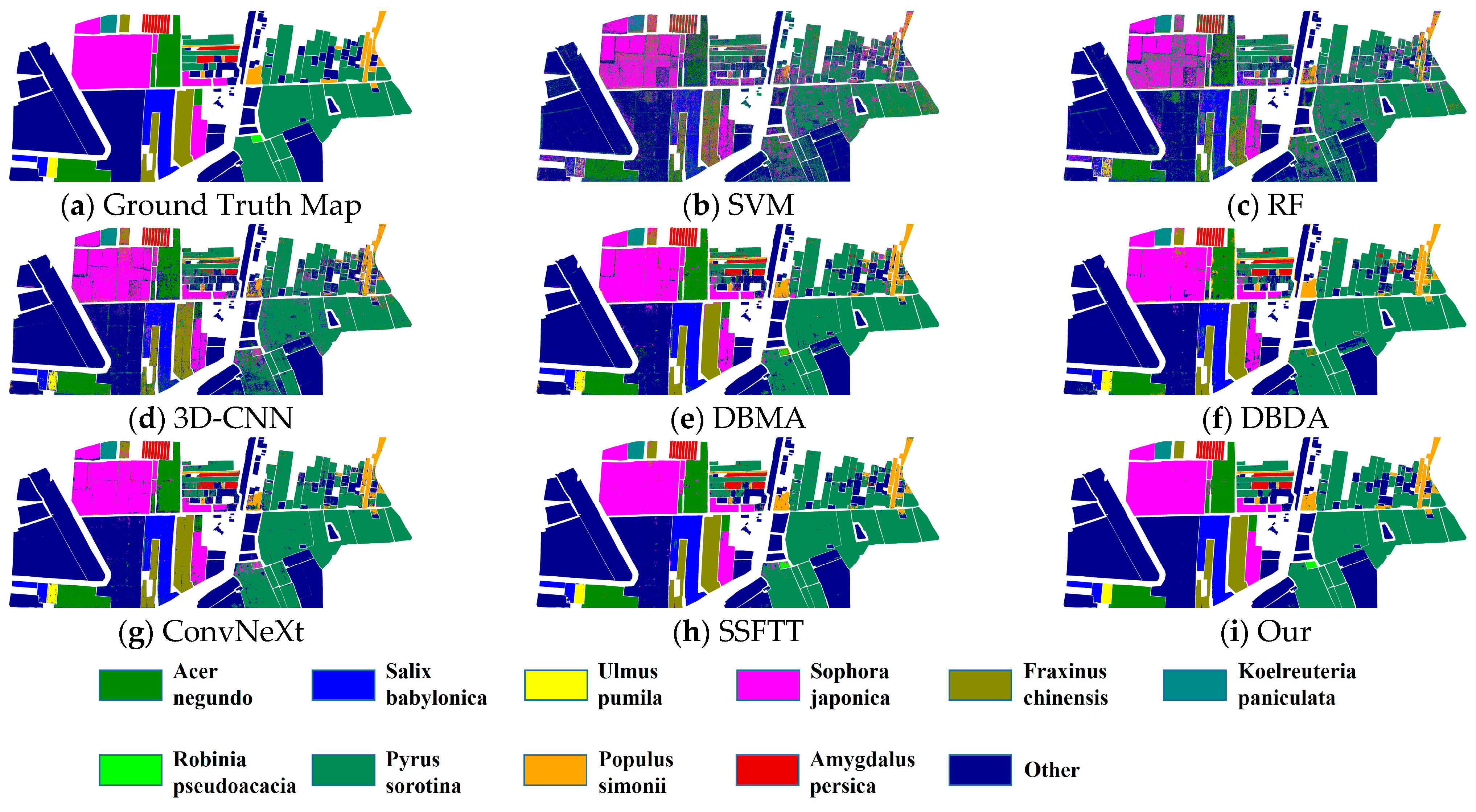
To demonstrate the superiority and effectiveness of the proposed method in this study, we compare it with traditional machine learning methods such as SVM and RF, and other state-of-the-art deep learning methods such as 3D-CNN, DBMA, DBDA, ConvNeXt and SSFTT. Next, the compared methods are briefly described separately.

1.

SVM: Support Vector Machine. A support vector machine with a radial basis function was used in this study, and the input features were important bands, vegetation index, the first three principal components after PCA dimensionality reduction, and eight spatial texture features corresponding to each principal component.

2.

RF: Random Forest. The parameter n_estimators was set to 500, and the input features were consistent with those of the SVM.

3.

3D-CNN: Three-Dimensional Convolutional Neural Network. The specific network architecture is described in Zhang et al. [27]. The method is based on the 3D-CNN, and the input data size is 1 × 9 × 9 × bands, where “band” represents the number of spectral bands, and 9 denotes patch size.

4.

DBMA: Double-Branch Multi-Attention Mechanism Network. The specific network architecture is described in Ma et al. [42]. The method is based on a double-branch network structure, dense blocks and the CBAM attention mechanism, and the input data size is consistent with a 3D-CNN.

5.

DBDA: Double-Branch Dual-Attention Mechanism Network. The specific network architecture is described in Li et al. [48]. The method is based on a double-branch network structure, dense blocks and the DANet attention mechanism, and the input data size is consistent with a 3D-CNN.

6.

ConvNeXt: A pure ConvNet model. The specific network architecture is described in Liu et al. [49]. The method is based on the ideas of ResNet and Swin Transformer, and the input data size is band × 9 × 9.

7.

SSFTT: Spectral–Spatial Feature Tokenization Transformer. The specific network architecture is described in Sun et al. [50]. The method is based on the 3D-CNN and Transformer Encoder. The input data size is 1 × 30 × 13 × 13, where 30 denotes the first thirty principal components after PCA dimensionality reduction, and 13 denotes patch size.

To fairly compare the classification performance of each deep learning method, we set the same training parameters. In particular, the batch size is set to 128, and the Adam optimizer is adopted. The learning rate is set to 0.0001, and we train each model for 50 epochs.

All methods were implemented in Python 3.6. SVM and RF were implemented based on the scikit-learn library, and deep learning methods were implemented based on the Pytorch 1.9.1 open-source deep learning framework. The operating platform configuration consisted of two Intel(R) Xeon(R) Gold 5218R @2.10GHz CPU (Intel Corporation, Santa Clara, CA, USA) and an NVIDIA GeForce RTX 3080 GPU (NVIDIA Corporation, Santa Clara, CA, USA).

4. Experiments

4.1. The Classification Results of the TEF Dataset

The classification results of the TEF dataset using different methods are shown in

Table 4. The classification results of different methods used on the TEF dataset.

Species	SVM	RF	3D-CNN	DBMA	DBDA	ConvNeXt	SSFTT	Our
abco	39.12%	66.12%	73.33%	79.03%	87.07%	78.83%	82.20%	88.40%
abma	7.11%	14.91%	25.29%	51.26%	85.24%	64.90%	76.14%	88.08%
cade	20.02%	60.09%	78.38%	86.46%	92.30%	89.42%	90.21%	93.76%
pije	48.04%	82.34%	84.73%	94.08%	96.13%	95.15%	96.05%	97.40%
pila	34.23%	83.10%	85.65%	93.07%	99.43%	93.63%	95.26%	98.87%
quke	12.68%	42.11%	53.12%	48.62%	76.72%	84.63%	68.51%	80.17%
pico	14.64%	47.07%	70.58%	82.19%	89.47%	87.96%	89.34%	90.94%
dead	83.30%	86.63%	85.33%	85.01%	87.59%	86.71%	85.40%	89.53%
OA	44.65%	73.18%	78.89%	86.18%	92.16%	88.13%	89.52%	93.31%
AA	32.39%	60.30%	69.55%	77.47%	89.24%	85.15%	85.39%	90.89%
Kappa	0.3158	0.6675	0.7418	0.8307	0.9043	0.8551	0.8721	0.9183

. It can be observed that all deep learning-based methods achieve higher classification accuracy compared to the traditional machine learning methods (SVM and RF). The SVM method achieved the lowest classification accuracy with an OA value of only 44.65%. Compared with other classification methods, the method proposed in this study achieved the highest classification accuracy, with an OA value of 93.31%, an AA value of 90.89%, and a Kappa coefficient of 0.9183. Except for Pinus lambertiana and Quercus kelloggii, the highest classification accuracy of other tree species was obtained using the proposed method. The highest classification accuracy (99.43%) for Pinus lambertiana was obtained using the DBDA method. The proposed method achieved the second-highest classification accuracy for Pinus lambertiana, with a classification accuracy of 98.87%, and the difference between these two methods was only 0.56%. Among all the tree species, the classification accuracy of Abies magnifica and Quercus kelloggii was relatively low, with most below 60%. Abies concolor and Abies magnifica both belong to the genus abies of the pine family, and their spectral information is similar. Additionally, as known from Table 1, the number of Abies magnifica pixels used for training was 718, only one-third of the number of Abies concolor pixels (2330). These two factors caused the mixed classification between the two tree species, which led to the lower classification accuracy of Abies magnifica. The number of Quercus kelloggii pixels used for training was only 96, and the serious shortage of training samples may be the main reason for its low classification accuracy. The proposed method achieved classification accuracy above 80% for both of these tree species, indicating that the method can obtain good classification results in the case of sample imbalance and limited training samples.

The hyperspectral image was predicted using the proposed method, and the classification map of the study area is shown in Figure 5. From the classification map, it can be observed that the most prevalent tree species in the study area are Abies concolor, Pinus jeffreyi, and Pinus contorta. Specifically, Abies concolor is mainly distributed in the northern (Figure 5b) and southern (Figure 5f) regions of the study area. Pinus jeffreyi is distributed in the northern (blue-colored area in Figure 5), central (Figure 5c), and southern (Figure 5e) regions of the study area. Pinus contorta is mainly distributed in the central region of the study area, as shown in Figure 5c,d.

4.2. The Classification Results of the Tiegang Reservoir Dataset

The classification results of the Tiegang Reservoir dataset using different methods are shown in

Table 5. The classification results of different methods used on the TieGang Reservoir dataset.

Species	SVM	RF	3D-CNN	DBMA	DBDA	ConvNeXt	SSFTT	Our
glpe	25.59%	76.77%	77.06%	83.39%	98.32%	91.08%	99.21%	98.54%
cica	83.56%	94.27%	96.07%	95.34%	97.99%	98.22%	97.72%	98.34%
euro	65.06%	89.10%	96.88%	96.90%	96.92%	97.18%	96.84%	97.65%
fial	2.48%	4.30%	14.25%	11.92%	19.09%	4.41%	19.14%	24.40%
plor	63.29%	86.59%	96.02%	94.66%	98.79%	92.45%	98.08%	99.58%
fimi	35.20%	66.10%	89.54%	91.07%	98.05%	84.05%	97.86%	98.97%
cahy	50.16%	86.82%	96.49%	98.60%	98.73%	98.01%	98.44%	99.64%
OA	64.77%	85.29%	91.21%	91.45%	94.97%	92.32%	94.76%	95.7%
AA	46.48%	71.99%	80.9%	81.70%	86.84%	80.77%	86.75%	88.16%
Kappa	0.4709	0.7874	0.875	0.8791	0.9284	0.8900	0.9255	0.9389

. Similarly, we observed that all deep learning-based methods achieve higher classification accuracy than traditional machine learning methods. This is because SVM and RF classifiers use shallow features of the dataset, which makes it difficult to distinguish complex classification objects such as tree species with similar spectral information, whereas deep learning methods automatically learn nonlinear high-level features from the training set, which provides a strong advantage in classifying hyperspectral tree species. Compared with other deep learning neural networks, the proposed method makes full use of the spectral and spatial information of hyperspectral images and minimizes the loss of information. The optimal accuracy of tree species classification was obtained using the proposed method with an OA value of 95.7%, an AA value of 88.16%, and a Kappa coefficient of 0.9389. Among all tree species, Ficus altissima species obtained the lowest classification accuracy, all were below 30%. The proposed method obtained the highest classification accuracy, but only of 24.4%. Compared with other tree species, fewer Ficus altissima samples were used for training, and the severe shortage in sample size is the most important reason for its lower classification accuracy.

The tree species prediction maps of the Tiegang Reservoir study area that were generated using deep learning methods are shown in Figure 6. From the classification maps, it can be observed that the distribution of different tree species is relatively concentrated, mainly in the form of pure forests. The areas of tree species predicted using the different methods are generally consistent. The classification maps obtained using the 3D-CNN and DBMA have more noise than other classification methods. The main dominant tree species in the study area are Cinnamomum camphora, Glyptostrobus pensilis, and Platycladus orientalis. Cinnamomum camphora is the most widely distributed tree species in the study area, with distribution across various regions. Glyptostrobus pensilis is mainly distributed in the southern region of the study area, closer to the reservoir. Platycladus orientalis is primarily distributed in the northwest region of the study area.

4.3. The Classification Results for the Xiongan New Area Dataset

The results of classifying the Xiongan New Area dataset using different methods are shown in

Table 6. The classification results of different methods used on the Xiongan New Area dataset.

Species	SVM	RF	3D-CNN	DBMA	DBDA	ConvNeXt	SSFTT	Our
acne	55.27%	62.28%	76.54%	87.58%	84.32%	90.13%	96.06%	98.64%
saba	53.58%	66.58%	74.93%	93.40%	93.86%	94.19%	98.02%	99.04%
ulpu	17.58%	45.44%	75.83%	89.31%	78.59%	94.26%	97.26%	99.43%
soja	62.91%	61.12%	80.93%	94.91%	91.10%	94.34%	99.04%	98.99%
frch	45.29%	41.97%	78.05%	94.45%	97.99%	93.81%	98.81%	99.49%
kopa	63.77%	76.99%	82.63%	95.93%	95.45%	93.39%	99.83%	99.88%
rops	1.30%	0.00%	1.43%	27.57%	0.00%	12.86%	66.43%	95.29%
pyso	72.37%	84.98%	85.80%	93.25%	95.84%	95.64%	98.39%	98.86%
posi	30.66%	43.27%	61.52%	81.66%	86.51%	81.75%	89.46%	93.33%
ampe	26.83%	35.35%	53.42%	84.06%	81.40%	87.85%	95.66%	96.43%
other	79.04%	85.61%	90.55%	95.22%	95.07%	96.73%	98.19%	99.11%
OA	68.22%	75.59%	84.15%	93.38%	93.52%	94.76%	97.94%	98.82%
AA	46.24%	54.87%	69.24%	85.21%	81.83%	84.99%	94.29%	98.04%
Kappa	0.5768	0.6699	0.7886	0.9119	0.9137	0.9301	0.9727	0.9843

. Similar to the results obtained from the TEF and Tiegang Reservoir datasets, all deep learning-based methods obtained higher classification accuracy than traditional machine learning methods. The proposed method achieved optimal accuracy compared to other deep learning methods, with an OA value of 98.82%, an AA value of 98.04%, and a Kappa coefficient of 0.9843, which far exceeded the classification performance of other methods. Among all tree species, the classification accuracy of Robinia pseudoacacia was the lowest, in which RF and DBDA methods could not separate Robinia pseudoacacia from other tree species, with a classification accuracy of 0.00%, and the classification accuracy of other classification methods was also lower than 30%. This was because the number of training samples for Robinia pseudoacacia was relatively small compared to other categories. As can be seen from Table 3, only 28 Robinia pseudoacacia samples were used for training, which makes it difficult for the classifier to learn distinguishable features. However, under the conditions of unbalanced samples and limited training samples, the proposed method can perform well in distinguishing Robinia pseudoacacia from other tree species, with a classification accuracy of 95.29%, which proves the robustness of the method.

The ground truth map and the classification maps, obtained using various methods, for the Xiongan New Area dataset are shown in Figure 7. Although each classifier can distinguish the boundaries between tree species well, different degrees of “salt and pepper” noise phenomenon exist. The “salt and pepper” noise in the classification map (Figure 7b) obtained using SVM is the most serious. The method proposed in this study not only uses the spectral information, but also makes full use of the spatial information of pixels. Compared to other methods, the phenomenon of “salt and pepper” noise is significantly improved, and the classification map (Figure 7i) is basically consistent with the ground truth map.

5. Discussion

5.1. The Importance of Joint Spatial–Spectral Features

In this study, a series of comparative experiments were conducted to discuss the importance of combining spatial–spectral information in the classification of spectral branch, spatial branch, and double-branch network structures.

In the spectral branch, the 3D convolution operation was changed to a 1D convolution operation, the input data was changed to the spectral information of the pixels to be classified, excluding the spectral information of their neighboring pixels, and other operations remained unchanged. Specifically, only the spectral information of pixels to be classified was considered in the spectral branch, and no spatial information was included. The spectral branch was to classify the tree species on the three datasets. For the TEF dataset, when the input of the spectral branch was only the spectral information of pixels to be classified (“Spectral single” in Figure 8), the OA value was 84.92%, and the AA value was 76.96%. However, when the spectral information of other pixels in the neighborhood was added (“Spectral” in Figure 8), the obtained OA value increased to 91.82% (an improvement of 6.9 percentage points), and the AA value increased to 87.87% (an improvement of 10.91 percentage points). Similar results were obtained for the Tiegang Reservoir and the Xiongan New Area datasets, with improvements in OA of 0.33% and 6.74%, respectively, when the spatial information was added to the spectral branch. The above experiments demonstrate the advantage of joint spatial–spectral information in the spectral branch. An individual tree generally occupies multiple pixels in airborne hyperspectral images with high spatial resolution. Therefore, the spectral information of pixels to be classified cannot be considered only when extracting features using the spectral branch, ignoring its spatial dependence with neighboring pixels. Reasonable use of the neighborhood information of pixels is helpful in improving the classification accuracy.

When using spatial information to classify hyperspectral tree species, the conventional method is first to reduce the dimension of the hyperspectral image, and then extract the spatial information of pixels from the data after dimensionality reduction to classify tree species. Following this approach, the input data of the spatial branch was modified to be the first three principal components data after PCA dimensionality reduction, and other operations remained unchanged. Specifically, the spatial information of pixels was mainly utilized in the spatial branch for classification. For the TEF dataset, when the input data of the spatial branch was the data after PCA dimensionality reduction (“Spatial PCA” in Figure 8), the obtained OA value was only 69.64%, and the AA value was 53.17%. However, when all of the original band information was selected to be input into the spatial branch (“Spatial” in Figure 8), the obtained OA value increased to 89.45% (an improvement of 19.81 percentage points), and the AA value increased to 84.74% (an improvement of 31.57 percentage points). Similar results were obtained with the other two datasets. When the input data of the spatial branch was the original band information, the OA values were improved by 25.06% and 7.65%, respectively, and the classification performance was better than the data after PCA reduction. During the process of PCA dimensionality reduction in hyperspectral data, although the spatial information of pixels will be retained, a certain amount of spectral information will be lost in the dimensionality reduction process. In contrast, the proposed method selects all of the original band information to be put into the network in the spatial branch, avoiding the loss of spectral information. The above experiments demonstrate the advantage of joint spatial–spectral information in the spatial branch.

Although the spectral branch and the spatial branch in this study both make use of the spatial–spectral information of hyperspectral data, the focus of feature extraction for the spectral branch and the spatial branch is different; the spectral branch focuses on extracting spectral features using a 3D-CNN (with convolution kernel of (1, 1, 7)) and the spatial branch focuses on extracting spatial features using a 2D-CNN (with convolution kernel of (3, 3)). Using only a single branch may not be able to utilize the advantages of the hyperspectral image fully. Therefore, a double-branch network was designed to fuse the two branches for tree species classification, which further utilizes spatial–spectral information. Taking the TEF dataset as an example, the proposed method achieved classification accuracy with an OA value of 93.31% and an AA value of 90.89%. Compared to the spectral branch (“Spectral” in Figure 8), there was an improvement of 1.49 percentage points in OA and 3.02 percentage points in AA. Compared to the spatial branch (“Spatial” in Figure 8), there was an improvement of 3.86 percentage points in OA and 6.15 percentage points in AA. Similar results were obtained for the other two tree species datasets. For the Tiegang Reservoir dataset, the proposed method outperforms the spectral branch (“Spectral” in Figure 9) by 0.82 percentage points and the spatial branch (“Spatial” in Figure 9) by 1.61 percentage points in terms of OA value. For the Xiongan New Area dataset, the proposed method outperforms the spectral branch (“Spectral” in Figure 10) by 1.48 percentage points and the spatial branch (“Spatial” in Figure 10) by 2.77 percentage points in terms of OA value. The above experiments demonstrate the advantages of the double-branch network in hyperspectral tree species classification. These findings are consistent with the experimental results obtained by Ma et al. [42] and Li et al. [48]. In practical tree species classification applications, due to the complexity and similarity of tree canopy structure, it is difficult to obtain ideal tree species classification results by simply using the spectral information or spatial structure of trees. The method proposed in this study fully utilizes the spectral and spatial information of trees, which is conducive to improving the accuracy of tree species classification in hyperspectral images.

5.2. The Effectiveness of the SimAM Attention Mechanism

In order to analyze the effect of the SimAM attention mechanism on tree species classification, the ablation experiment of the attention mechanism was conducted, that is, the classification results of tree species with and without the attention mechanism network were compared. The comparison results of the three datasets are shown in

Table 7. Ablation experiment results of the SimAM attention mechanism.

Dataset Name	Method	OA Value	AA Value	Kappa Value
TEF dataset	No Attention	92.02%	88.6%	0.9025
	Attention	93.31%	90.89%	0.9183
Tiegang Reservoir dataset	No Attention	95.1%	87.35%	0.9303
	Attention	95.7%	88.16%	0.9389
Xiongan New Area dataset	No Attention	97.78%	94.31%	0.9705
	Attention	98.82%	98.04%	0.9843

. For the TEF dataset, the inclusion of the SimAM attention mechanism in the network resulted in an improvement of 1.29 percentage points in OA and 2.29 percentage points in AA. Similarly, the OA values obtained in the Tiegang Reservoir and the Xiongan New Area datasets improved by 0.6% and 1.04%, respectively. These results prove the effectiveness of introducing the SimAM attention mechanism into our proposed method. The attention mechanism can extract important features by assigning different weights to each part of the feature maps, thus effectively improving the classification accuracy of tree species.

5.3. The Influence of Shallow Features on Tree Species Classification

In this study, we used the neural network to extract deep features of data for tree species classification. However, in previous studies, many scholars used artificially extracted shallow features for classification. Figure 11 illustrates the shallow feature differences between the various tree species. As in NDVI, there are significant differences between the “Dead tree” category and other tree species. So, whether adding shallow features (Vegetation Index, PCA principal component, etc.) to the neural network will improve the classification results needs to be further verified. Therefore, we designed two different schemes. One way is to add shallow features to the head of the neural network, as shown in Figure 12a. First, the shallow features are extracted within a neighborhood (9 × 9) of pixels, then they are merged with the corresponding raw spatial–spectral information, and finally, the merged features are inputted into the neural network for classification. Another way is to add shallow features at the end of the neural networks, as shown in Figure 12b. First, the raw spatial–spectral information of pixels is inputted into the network to generate corresponding deep features, then the shallow features of pixels are merged with the extracted deep features, and finally, the two features are further fused through the fully connected layer to complete the classification.

We used the input features of traditional machine learning methods (SVM and RF) as shallow features and conducted experiments on three datasets. The classification results obtained are shown in Figure 13. In the three datasets, whether at the head or end of the networks, adding shallow features did not significantly improve the classification accuracy and even showed a decrease. The result is consistent with the findings of Nezami et al. [51], who added Canopy Height Model (CHM) features to the networks for classification and showed that adding CHM did not improve the classification accuracy in most cases. The reason for this phenomenon may be that the relevant information needed to separate the tree species is already contained by deep features, while shallow features are low-level features of images. If too many shallow features are added to the neural networks, it will interfere with the neural network’s learning of the higher-level features, thus affecting the classification accuracy. Combining shallow features with spectral features from hyperspectral data as inputs to the neural network may also lead to feature redundancy and increase the number of model parameters, resulting in overfitting of the model and negatively affecting the performance of the neural networks.

5.4. T-SNE Visualization

The T-distributed Stochastic Neighbor Embedding (T-SNE) algorithm is currently one of the most commonly employed techniques for data dimensionality reduction and visualization, which can reduce high-dimensional data to two-dimensional or three-dimensional data for visualization, and then can intuitively show the effect of tree species classification. In this study, the T-SNE algorithm was used to visualize the features extracted by the neural network. The visualization results obtained from the three datasets are shown in Figure 14, Figure 15 and Figure 16. For the TEF dataset, it can be seen that the features extracted using the 3D-CNN method are more dispersed, and there is more mixing between the categories compared to other classification methods, which leads to lower classification accuracy. The phenomenon of spectral variability within the same object occurs during the imaging process of targets by hyperspectral sensors due to factors such as the influence of tree growth environment and individual tree position. For instance, Calocedrus decurrens and Pinus contorta are divided into multiple clusters in DBMA and DBDA. Although these two methods achieve high overall classification accuracy, they cannot solve the phenomenon of spectral variability within the same object. The ConvNeXt and the proposed method alleviate this phenomenon to some extent, in which the trees of the same class are basically grouped into a cluster. The boundaries between each category of ConvNeXt are clear, but the mixing phenomenon between various categories is more serious, such as the mixing between Abies concolor and Abies magnifica, Pinus jeffreyi, and Pinus lambertiana. From the visualization results of the method proposed in this study, it can be seen that the boundaries between the categories are clear, and there is less mixing between the categories, which explains why the method achieves the highest accuracy. The visualization effects obtained from the Tiegang reservoir and the Xiongan New Area datasets are similar to those obtained from the TEF dataset, that is, the proposed method performs best in T-SNE visualization compared with other methods, with clear classification boundaries among tree species and fewer misclassified pixels.

5.5. Robustness Assessment

Deep learning is a data-driven algorithm that relies on high-quality labeled datasets. The number or proportion of training samples is one of the important factors affecting classification accuracy. In this study, deep learning methods were trained with different proportions of training samples to verify the robustness of the proposed method. Specifically, the ratios of training sets and test sets selected for the TEF and the Tiegang Reservoir datasets were 2:8, 4:6, 5:5, 6:4, and 8:2, respectively. The training sets selected for the Xiongan New Area dataset were 0.1%, 0.5%, 1%, 2%, and 5% of the entire sample set, respectively, and the test set was unified into 5% of the sample set. The classification results obtained are shown in Figure 17.

It can be observed that different proportions of training samples yield different classification results. As expected in this study, in most cases, the performance of the network model improves as the proportion of training samples increases. The performance gap between different models will decrease with the increase in the proportion of training samples. The most obvious is the Xiongan New Area dataset. When the proportion of training samples is 0.1%, the performance gap between the 3D-CNN and the proposed method is as high as 28.53 percentage points. However, as the proportion of training samples reaches 5%, the performance gap narrows to 3.67 percentage points. In addition, the proposed method achieves the highest accuracy with different proportions of training samples in all three datasets. In the Xiongan New Area dataset, the classification accuracy obtained using the proposed method is as high as 99.97% when the proportion of training samples is 5%. Compared with other methods, the classification performance of the method in this study is more stable under different proportions of training samples, and the classification accuracy does not change drastically with different proportions of training samples, which indicates that the model is robust to changes in the training data.

The proposed method exhibits commendable performance even with limited training samples. Specifically, the classification accuracy obtained using the proposed method on the TEF dataset and the Tiegang Reservoir dataset is 88.83% and 91.79%, respectively, when the ratio of the training set to the test set is 2:8. For the Xiongan New Area dataset, when the proportion of the training set is 0.1% of the sample set, the classification accuracy obtained is 95.49%, which is much better than the performance of other models. During the actual collection of tree species samples, obtaining a large number of samples is challenging due to factors such as the complexity and limited accessibility of forest areas. The difficulties and high costs associated with sample acquisition make it impractical to gather a substantial dataset. However, the proposed method achieves a high classification performance even with limited training samples, thereby saving time and reducing costs. This approach proves to be suitable for scenarios with limited sample availability.

6. Conclusions

In this study, we combine the ideas of the attention mechanism and double-branch network structure to propose a double-branch spatial–spectral joint deep learning network for airborne hyperspectral tree species classification. Compared with other classification methods, the network shows better robustness in three tree species datasets. Experimental results are shown the following:

1.

In hyperspectral tree species classification, deep learning methods are better than traditional machine learning methods (SVM and RF) in distinguishing tree species, and the method proposed in this study achieved the highest classification accuracy in all three study areas. The OA value, AA value, and Kappa coefficient in the TEF dataset were 93.31%, 90.89%, and 0.9183, respectively. The OA value, AA value, and Kappa coefficient in the Tiegang reservoir dataset were 95.7%, 88.16%, and 0.9389, respectively. The OA value, AA value, and Kappa coefficient in the Xiongan New Area dataset were 98.82%, 98.04%, and 0.9843, respectively.

2.

Using only the spectral or spatial information of pixels cannot fully utilize the advantages of hyperspectral images, and the combined spectral and spatial information can help to improve the accuracy of tree species classification. The double-branch network structure is better than the single-branch network in terms of tree species classification performance. Furthermore, the SimAM attention mechanism can make the network pay more attention to important features and then improve the network classification performance, which proves the effectiveness of the SimAM attention mechanism in high-precision tree species classification in forest areas.

3.

The proposed method performs best in T-SNE visualization, with clear classification boundaries between tree species and fewer misclassified pixels. The method obtains the highest accuracy under different training sample proportions, and good classification performance can be obtained even under the lowest training sample proportions. Moreover, the classification accuracy does not change drastically with different training sample proportions, which are somewhat stable.

The proposed network fully utilizes the spectral and spatial information of hyperspectral images to realize the high-precision classification of forest tree species, which has a broad application prospect in forest resources investigation. However, the method has limitations in limited samples classification and crown level classification. In the future, we will investigate semi-supervised classification algorithms to solve the case of few-shot samples based on this method. In addition, trees have unique properties, the same tree contains multiple pixels in high-resolution images from airborne or unmanned aerial vehicles (UAV). Therefore, tree species classification at the crown level may help to improve the classification results. In subsequent experiments, we will conduct tree species classification studies based on the crown level.

References

1. Wiens, J.J. Climate-Related Local Extinctions Are Already Widespread among Plant and Animal Species. PLoS Biol. 2016, 14, e2001104. [Google Scholar] [CrossRef]
2. Fassnacht, F.E.; Latifi, H.; Sterenczak, K.; Modzelewska, A.; Lefsky, M.; Waser, L.T.; Straub, C.; Ghosh, A. Review of studies on tree species classification from remotely sensed data. Remote Sens. Environ. 2016, 186, 64–87. [Google Scholar] [CrossRef]
3. Meng, R.; Wu, J.; Zhao, F.; Cook, B.D.; Hanavan, R.P.; Serbin, S.P. Measuring short-term post-fire forest recovery across a burn severity gradient in a mixed pine-oak forest using multi-sensor remote sensing techniques. Remote Sens. Environ. 2018, 210, 282–296. [Google Scholar] [CrossRef]
4. Jactel, H.; Moreira, X.; Castagneyrol, B. Tree Diversity and Forest Resistance to Insect Pests: Patterns, Mechanisms, and Prospects. In Annual Review of Entomology; Douglas, A.E., Ed.; Annual Reviews: San Mateo, CA, USA, 2021; Volume 66, pp. 277–296. [Google Scholar]
5. Nascimento, W.R.; Souza, P.W.M.; Proisy, C.; Lucas, R.M.; Rosenqvist, A. Mapping changes in the largest continuous Amazonian mangrove belt using object-based classification of multisensor satellite imagery. Estuar. Coast. Shelf Sci. 2013, 117, 83–93. [Google Scholar] [CrossRef]
6. Kampouri, M.; Kolokoussis, P.; Argialas, D.; Karathanassi, V. Mapping of forest tree distribution and estimation of forest biodiversity using Sentinel-2 imagery in the University Research Forest Taxiarchis in Chalkidiki, Greece. Geocarto Int. 2019, 34, 1273–1285. [Google Scholar] [CrossRef]
7. Modzelewska, A.; Fassnacht, F.E.; Sterenczak, K. Tree species identification within an extensive forest area with diverse management regimes using airborne hyperspectral data. Int. J. Appl. Earth Obs. Geoinf. 2020, 84, 101960. [Google Scholar] [CrossRef]
8. Alzubaidi, L.; Zhang, J.L.; Humaidi, A.J.; Al-Dujaili, A.; Duan, Y.; Al-Shamma, O.; Santamaria, J.; Fadhel, M.A.; Al-Amidie, M.; Farhan, L. Review of deep learning: Concepts, CNN architectures, challenges, applications, future directions. J. Big Data 2021, 8, 53. [Google Scholar] [CrossRef]
9. Paoletti, M.E.; Haut, J.M.; Plaza, J.; Plaza, A. Deep learning classifiers for hyperspectral imaging: A review. ISPRS J. Photogramm. Remote Sens. 2019, 158, 279–317. [Google Scholar] [CrossRef]
10. Bolyn, C.; Lejeune, P.; Michez, A.; Latte, N. Mapping tree species proportions from satellite imagery using spectral-spatial deep learning. Remote Sens. Environ. 2022, 280, 113205. [Google Scholar] [CrossRef]
11. Abbas, S.; Peng, Q.; Wong, M.S.; Li, Z.L.; Wang, J.C.; Ng, K.T.K.; Kwok, C.Y.T.; Hui, K.K.W. Characterizing and classifying urban tree species using bi-monthly terrestrial hyperspectral images in Hong Kong. ISPRS J. Photogramm. Remote Sens. 2021, 177, 204–216. [Google Scholar] [CrossRef]
12. Zhang, M.M.; Li, W.; Zhao, X.D.; Liu, H.; Tao, R.; Du, Q. Morphological Transformation and Spatial-Logical Aggre-gation for Tree Species Classification Using Hyperspectral Imagery. IEEE Trans. Geosci. Remote Sens. 2023, 61, 5501212. [Google Scholar] [CrossRef]
13. Huang, G.; Liu, Z.; van der Maaten, L.; Weinberger, K.Q. Densely Connected Convolutional Networks. In Proceedings of the 30TH IEEE Conference on Computer Vision and Pattern Recognition (CVPR 2017), Honolulu, HI, USA, 21–26 July 2017; IEEE: Piscataway, NJ, USA, 2017; pp. 2261–2269. [Google Scholar]
14. Ren, S.Q.; He, K.M.; Girshick, R.; Sun, J. Faster R-CNN: Towards Real-Time Object Detection with Region Proposal Networks. In Proceedings of the Advances in Neural Information Processing Systems 28 (NIPS 2015), Montreal, QC, Canada, 7–12 December 2015. [Google Scholar]
15. Long, J.; Shelhamer, E.; Darrell, T. Fully Convolutional Networks for Semantic Segmentation. In Proceedings of the 2015 IEEE Conference on Computer Vision and Pattern Recognition (CVPR), Boston, MA, USA, 7–12 June 2015; IEEE: Piscataway, NJ, USA, 2015; pp. 3431–3440. [Google Scholar]
16. Li, Q.S.; Wong, F.K.K.; Fung, T. Mapping multi-layered mangroves from multispectral, hyperspectral, and LiDAR data. Remote Sens. Environ. 2021, 258, 112403. [Google Scholar] [CrossRef]
17. La Rosa, L.E.C.; Sothe, C.; Feitosa, R.Q.; de Almeida, C.M.; Schimalski, M.B.; Oliveira, D.A.B. Multi-task fully convolutional network for tree species mapping in dense forests using small training hyperspectral data. ISPRS J. Photogramm. Remote Sens. 2021, 179, 35–49. [Google Scholar] [CrossRef]
18. Zhao, H.W.; Zhong, Y.F.; Wang, X.Y.; Hu, X.; Luo, C.; Boitt, M.; Piiroinen, R.; Zhang, L.P.; Heiskanen, J.; Pellikka, P. Mapping the distribution of invasive tree species using deep one-class classification in the tropical montane land-scape of Kenya. ISPRS J. Photogramm. Remote Sens. 2022, 187, 328–344. [Google Scholar] [CrossRef]
19. Wei, X.P.; Yu, X.C.; Liu, B.; Zhi, L. Convolutional neural networks and local binary patterns for hyperspectral image classification. Eur. J. Remote Sens. 2019, 52, 448–462. [Google Scholar] [CrossRef]
20. Cai, J.N.; Meng, L.; Liu, H.L.; Chen, J.; Xing, Q.G. Estimating Chemical Oxygen Demand in estuarine urban rivers using unmanned aerial vehicle hyperspectral images. Ecol. Indic. 2022, 139, 108936. [Google Scholar] [CrossRef]
21. Xi, Y.B.; Ren, C.Y.; Wang, Z.M.; Wei, S.Q.; Bai, J.L.; Zhang, B.; Xiang, H.X.; Chen, L. Mapping Tree Species Composition Using OHS-1 Hyperspectral Data and Deep Learning Algorithms in Changbai Mountains, Northeast China. Forests 2019, 10, 818. [Google Scholar] [CrossRef]
22. Sothe, C.; De Almeida, C.M.; Schimalski, M.B.; La Rosa, L.E.C.; Castro, J.D.B.; Feitosa, R.Q.; Dalponte, M.; Lima, C.L.; Liesenberg, V.; Miyoshi, G.T.; et al. Comparative performance of convolutional neural network, weighted and conventional support vector machine and random forest for classifying tree species using hyperspectral and photogrammetric data. GIScience Remote Sens. 2020, 57, 369–394. [Google Scholar] [CrossRef]
23. Xu, Y.H.; Du, B.; Zhang, F.; Zhang, L.P. Hyperspectral image classification via a random patches network. ISPRS J. Photogramm. Remote Sens. 2018, 142, 344–357. [Google Scholar] [CrossRef]
24. Fricker, G.A.; Ventura, J.D.; Wolf, J.A.; North, M.P.; Davis, F.W.; Franklin, J. A Convolutional Neural Network Classifier Identifies Tree Species in Mixed-Conifer Forest from Hyperspectral Imagery. Remote Sens. 2019, 11, 2326. [Google Scholar] [CrossRef]
25. Mayra, J.; Keski-Saari, S.; Kivinen, S.; Tanhuanpaa, T.; Hurskainen, P.; Kullberg, P.; Poikolainen, L.; Viinikka, A.; Tuominen, S.; Kumpula, T.; et al. Tree species classification from airborne hyperspectral and LiDAR data using 3D convolutional neural networks. Remote Sens. Environ. 2021, 256, 112322. [Google Scholar] [CrossRef]
26. Zhou, J.B.; Zeng, S.; Gao, G.Q.; Chen, Y.L.; Tang, Y.Y. A Novel Spatial–Spectral Pyramid Network for Hyperspectral Image Classification. IEEE Trans. Geosci. Remote Sens. 2023, 61, 5519314. [Google Scholar]
27. Zhang, B.; Zhao, L.; Zhang, X.L. Three-dimensional convolutional neural network model for tree species classification using airborne hyperspectral images. Remote Sens. Environ. 2020, 247, 111938. [Google Scholar] [CrossRef]
28. Shi, C.P.; Liao, D.L.; Xiong, Y.; Zhang, T.Y.; Wang, L.G. Hyperspectral Image Classification Based on Dual-Branch Spectral Multiscale Attention Network. IEEE J. Sel. Top. Appl. Earth Obs.-Tions Remote Sens. 2021, 14, 10450–10467. [Google Scholar] [CrossRef]
29. Zhang, H.K.; Li, Y.; Zhang, Y.Z.; Shen, Q. Spectral-spatial classification of hyperspectral imagery using a dual-channel convolutional neural network. Remote Sens. Lett. 2017, 8, 438–447. [Google Scholar] [CrossRef]
30. Chen, R.; Li, G.H.; Dai, C.L. DRGCN: Dual Residual Graph Convolutional Network for Hyperspectral Image Classi-fication. IEEE Geosci. Remote Sens. Lett. 2022, 19, 6009205. [Google Scholar] [CrossRef]
31. Liang, J.; Li, P.S.; Zhao, H.; Han, L.; Qu, M.L. Forest Species Classification of UAV Hyperspectral Image Using Deep Learning. In Proceedings of the 2020 Chinese Automation Congress (CAC 2020), Shanghai, China, 6–8 November 2020; IEEE: Piscataway, NJ, USA, 2020; pp. 7126–7130. [Google Scholar]
32. Liu, X.; Frey, J.; Munteanu, C.; Still, N.; Koch, B. Mapping tree species diversity in temperate montane forests using Sentinel-1 and Sentinel-2 imagery and topography data. Remote Sens. Environ. 2023, 292, 113576. [Google Scholar] [CrossRef]
33. Clark, M.L. Comparison of multi-seasonal Landsat 8, Sentinel-2 and hyperspectral images for mapping forest alliances in Northern California. ISPRS J. Photogramm. Remote Sens. 2020, 159, 26–40. [Google Scholar] [CrossRef]
34. Ferreira, M.P.; Wagner, F.H.; Aragao, L.; Shimabukuro, Y.E.; de Souza, C.R. Tree species classification in tropical forests using visible to shortwave infrared WorldView-3 images and texture analysis. ISPRS J. Photogramm. Remote Sens. 2019, 149, 119–131. [Google Scholar] [CrossRef]
35. Park, J.Y.; Muller-Landau, H.C.; Lichstein, J.W.; Rifai, S.W.; Dandois, J.P.; Bohlman, S.A. Quantifying Leaf Phenology of Individual Trees and Species in a Tropical Forest Using Unmanned Aerial Vehicle (UAV) Images. Remote Sens. 2019, 11, 1534. [Google Scholar] [CrossRef]
36. Grabska, E.; Frantz, D.; Ostapowicz, K. Evaluation of machine learning algorithms for forest stand species mapping using Sentinel-2 imagery and environmental data in the Polish Carpathians. Remote Sens. Environ. 2020, 251, 112103. [Google Scholar] [CrossRef]
37. Qin, H.M.; Zhou, W.Q.; Yao, Y.; Wang, W.M. Individual tree segmentation and tree species classification in subtropical broadleaf forests using UAV-based LiDAR, hyperspectral, and ultrahigh-resolution RGB data. Remote Sens. Environ. 2022, 280, 113143. [Google Scholar] [CrossRef]
38. Marconi, S.; Weinstein, B.; Zou, S.; Bohlman, S.A.; Zare, A.; Singh, A.; Stewart, D.; Harmon, I.; Steinkraus, A.; White, E.P. Continental-scale hyperspectral tree species classification in the United States National Ecological Observatory Network. Remote Sens. Environ. 2022, 282, 113264. [Google Scholar] [CrossRef]
39. Hartling, S.; Sagan, V.; Maimaitijiang, M. Urban tree species classification using UAV-based multi-sensor data fusion and machine learning. GIScience Remote Sens. 2021, 58, 1250–1275. [Google Scholar] [CrossRef]
40. Dalponte, M.; Orka, H.O.; Gobakken, T.; Gianelle, D.; Naeesset, E. Tree Species Classification in Boreal Forests with Hyperspectral Data. IEEE Trans. Geosci. Remote Sens. 2013, 51, 2632–2645. [Google Scholar] [CrossRef]
41. Wei, L.F.; Wang, K.; Lu, Q.K.; Liang, Y.J.; Li, H.B.; Wang, Z.X.; Wang, R.; Cao, L.Q. Crops Fine Classification in Airborne Hyperspectral Imagery Based on Multi-Feature Fusion and Deep Learning. Remote Sens. 2021, 13, 2917. [Google Scholar] [CrossRef]
42. Ma, W.P.; Yang, Q.F.; Wu, Y.; Zhao, W.; Zhang, X.R. Double-Branch Multi-Attention Mechanism Network for Hyperspectral Image Classification. Remote Sens. 2019, 11, 1307. [Google Scholar] [CrossRef]
43. Hu, J.; Shen, L.; Sun, G. Squeeze-and-Excitation Networks. In Proceedings of the 2018 IEEE/CVF Conference on Computer Vision and Pattern Recognition (CVPR), Salt Lake City, UT, USA, 18–23 June 2018; IEEE: Piscataway, NJ, USA, 2018; pp. 7132–7141. [Google Scholar]
44. Wang, F.; Jiang, M.; Qian, C.; Yang, S.; Li, C.; Zhang, H.; Wang, X.; Tang, X. Residual Attention Network for Image Classification. In Proceedings of the 2017 IEEE Conference on Computer Vision and Pattern Recognition (CVPR), Honolulu, HI, USA, 21–26 July 2017; pp. 6450–6458. [Google Scholar]
45. Woo, S.; Park, J.; Lee, J.-Y.; Kweon, I.S. CBAM: Convolutional Block Attention Module. In Proceedings of the European Conference on Computer Vision (ECCV), Munich, Germany, 4–14 September 2018; Springer: Cham, Switzerland, 2018; pp. 3–19. [Google Scholar]
46. He, K.M.; Zhang, X.Y.; Ren, S.Q.; Sun, J. Deep Residual Learning for Image Recognition. In Proceedings of the 2016 IEEE Conference on Computer Vision and Pattern Recognition (CVPR), Las Vegas, NV, USA, 27–30 June 2016; IEEE: Piscataway, NJ, USA, 2016; pp. 770–778. [Google Scholar]
47. Yang, L.X.; Zhang, R.Y.; Li, L.D.; Xie, X.H. SimAM: A Simple, Parameter-Free Attention Module for Convolutional Neural Networks. In Proceedings of the International Conference on Machine Learning, Virtual Event, 13–15 December 2021; Volume 139. [Google Scholar]
48. Li, R.; Zheng, S.Y.; Duan, C.X.; Yang, Y.; Wang, X.Q. Classification of Hyperspectral Image Based on Double-Branch Dual-Attention Mechanism Network. Remote Sens. 2020, 12, 582. [Google Scholar] [CrossRef]
49. Liu, Z.; Mao, H.Z.; Wu, C.Y.; Feichtenhofer, C.; Darrell, T.; Xie, S.N. A ConvNet for the 2020s. In Proceedings of the 2022 IEEE/CVF Conference on Computer Vision and Pattern Recognition (CVPR), New Orleans, LA, USA, 18–24 June 2022; IEEE: Piscataway, NJ, USA, 2022; pp. 11966–11976. [Google Scholar]
50. Sun, L.; Zhao, G.R.; Zheng, Y.H.; Wu, Z.B. SpectralSpatial Feature Tokenization Transformer for Hyperspectral Image Classification. IEEE Trans. Geosci. Remote Sens. 2022, 60, 5522214. [Google Scholar] [CrossRef]
51. Nezami, S.; Khoramshahi, E.; Nevalainen, O.; Polonen, I.; Honkavaara, E. Tree Species Classification of Drone Hyperspectral and RGB Imagery with Deep Learning Convolutional Neural Networks. Remote Sens. 2020, 12, 1070. [Google Scholar] [CrossRef]
Figure 1. Location of TEF study area and the corresponding hyperspectral image.
Remotesensing 15 05679 g001
Figure 2. Location of TieGang Reservoir study area and the corresponding hyperspectral image.
Remotesensing 15 05679 g002
Figure 3. Location of Xiongan New Area study area and the corresponding hyperspectral image and ground truth map.
Remotesensing 15 05679 g003
Figure 4. Structure of a double-branch spatial–spectral joint network based on the SimAM attention mechanism.
Remotesensing 15 05679 g004
Figure 5. Classification maps of the proposed method used on the TEF dataset. Images (af) are partial enlargements of the tree species distribution. (a) Mixed forests of Abies concolor, Abies magnifica, and Pinus jeffreyi; (b) Abies concolor; (c) mixed forests of Abies concolor, Pinus jeffreyi, and Pinus contorta; (d) mixed forests of Abies magnifica, Pinus contorta, and dead tree; (e) mixed forests of Abies concolor, Calocedrus decurrens, and Pinus jeffreyi; (f) mixed forests of Abies concolor and Calocedrus decurrens.
Remotesensing 15 05679 g005
Figure 6. Classification maps obtained using different methods for the TieGang Reservoir dataset. Images (af) are the classification maps obtained using different methods.
Remotesensing 15 05679 g006
Figure 7. Classification maps obtained using different methods on the Xiongan New Area dataset. The first image (a) represents the ground truth map; images (bi) are the classification maps obtained via different methods.
Remotesensing 15 05679 g007
Figure 8. Experiments of spatial–spectral joint classification on the TEF dataset. “Spectral single” represents that only spectral information is used in Spectral Branch; “Spectral” represents that spatial–spectral information is used in Spectral Branch; “Spatial PCA” represents that only spatial information is used in Spatial Branch; “Spatial” represents that spatial–spectral information is used in Spatial Branch; “Our” represents the method proposed in this study.
Remotesensing 15 05679 g008
Figure 9. Experiments of spatial–spectral joint classification on the Tiegang Reservoir dataset. “Spectral single” represents that only spectral information is used in Spectral Branch; “Spectral” represents that spatial–spectral information is used in Spectral Branch; “Spatial PCA” represents that only spatial information is used in Spatial Branch; “Spatial” represents that spatial–spectral information is used in Spatial Branch; “Our” represents the method proposed in this study.
Remotesensing 15 05679 g009
Figure 10. Experiments of spatial–spectral joint classification on the Xiongan New Area dataset. “Spectral single” represents that only spectral information is used in Spectral Branch; “Spectral” represents that spatial–spectral information is used in Spectral Branch; “Spatial PCA” represents that only spatial information is used in Spatial Branch; “Spatial” represents that spatial–spectral information is used in Spatial Branch; “Our” represents the method proposed in this study.
Remotesensing 15 05679 g010
Figure 11. Boxplots of shallow features (The labels in the abscissa are abbreviations of tree species name, the scientific names are given in Table 1, and the different colors correspond to the different tree species). (a) NDVI: Normalized Difference Vegetation Index. (b) PC1: First principal component after PCA dimensionality reduction. (c) Mean: Mean texture features corresponding to the first principal component.
Remotesensing 15 05679 g011
Figure 12. The ways in which the neural network adds shallow features. (a) Add at the head of the neural network. (b) Add at the end of the neural network.
Remotesensing 15 05679 g012
Figure 13. Classification performance of incorporating shallow features in three datasets. (a) TEF Dataset; (b) Tiegang Reservoir Dataset; (c) Xiongan New Area Dataset.
Remotesensing 15 05679 g013
Figure 14. T-SNE visualization results on the TEF dataset. (a) 3D-CNN; (b) DBMA; (c) DBDA; (d) ConvNeXt; (e) SSFTT; (f) Our method.
Remotesensing 15 05679 g014
Figure 15. T-SNE visualization results on the Tiegang Reservoir dataset. (a) 3D-CNN; (b) DBMA; (c) DBDA; (d) ConvNeXt; (e) SSFTT; (f) Our method.
Remotesensing 15 05679 g015
Figure 16. T-SNE visualization results on the Xiongan New Area dataset. (a) 3D-CNN; (b) DBMA; (c) DBDA; (d) ConvNeXt; (e) SSFTT; (f) Our method.
Remotesensing 15 05679 g016aRemotesensing 15 05679 g016b
Figure 17. Classification performance of different training sample proportions on three datasets. (a) TEF Dataset; (b) Tiegang Reservoir Dataset; (c) Xiongan New Area Dataset.
Remotesensing 15 05679 g017