Article

Satellite Estimation of pCO2 and Quantification of CO2 Fluxes in China’s Chagan Lake in the Context of Climate Change

1
School of Geomatics and Prospecting Engineering, Jilin Jianzhu University, Changchun 130118, China
2
Northeast Institute of Geography and Agroecology, Chinese Academy of Sciences, Changchun 130102, China
3
School of Environment and Planning, Liaocheng University, Liaocheng 252000, China
*
Author to whom correspondence should be addressed.
Remote Sens. 2023, 15(24), 5680; https://doi.org/10.3390/rs15245680
Submission received: 27 October 2023 / Revised: 30 November 2023 / Accepted: 7 December 2023 / Published: 10 December 2023

Abstract

:
The massive increase in the amount of greenhouse gases in the atmosphere, especially carbon dioxide (CO2), has had a significant impact on the global climate. Research has revealed that lakes play an important role in the global carbon cycle and that they can shift between the roles of carbon sources and sinks. This study used Landsat satellite images to analyze the spatiotemporal characteristics and factors influencing the CO2 changes in Chagan Lake in China. We conducted six water sampling campaigns at Chagan Lake in 2020–2021 and determined the partial pressure of carbon dioxide (pCO2) from 110 water samples. Landsat surface reflectance was matched with water sampling events within ±7 days of satellite overpasses, yielding 75 matched pairs. A regression analysis indicated strong associations between pCO2 and both the band difference model of the near-infrared band and green band (Band 5-Band 3, R2 = 0.83, RMSE = 27.55 μatm) and the exponential model [((exp(b3) − exp(b5))2/(exp(b3) + exp(b5))2, R2 = 0.82, RMSE = 27.99 μatm]. A comparison between the performances of a linear regression model and a machine learning model found that the XGBoost model had the highest fitting accuracy (R2 = 0.94, RMSE = 16.86 μatm). We used Landsat/OLI images acquired mainly in 2021 to map pCO2 in Chagan Lake during the ice-free period. The pCO2 in the surface water of Chagan Lake showed considerable spatiotemporal variability within a range of 0–200 μatm. pCO2 also showed significant seasonal variations, with the lowest and highest mean values in autumn (30–50 μatm) and summer (120–150 μatm), respectively. Spatially, the pCO2 values in the southeast of Chagan Lake were higher than those in the northwest. The CO2 fluxes were calculated based on the pCO2 and ranged from −3.69 to −2.42 mmol/m2/d, indicating that Chagan Lake was absorbing CO2 (i.e., it was a weak carbon sink). Temperature, chlorophyll a, total suspended matter, and turbidity were found to have reinforcing effects on the overall trend of pCO2, while the Secchi disk depth was negatively correlated with pCO2. The results of this study provide valuable insights for assessing the role of lakes in the carbon cycle in the context of climate change.

1. Introduction

For decades, the release of greenhouse gases (GHGs), especially carbon dioxide (CO2), into the atmosphere by human activities and environmental changes has increased dramatically [1,2]. There is a consensus that the greenhouse effect caused by the continuous rise in atmospheric CO2 concentration is the principal factor causing global climatic change, which is seriously threatening sustainable societal and economic development [3]. The reduction in GHGs has become a critical topic of intense research focus [4,5,6].
A large number of studies have shown that lakes, as important contributors to inland waters, play a nonnegligible role in the global carbon cycle [7]. Although the total surface area of global lakes accounts for only 3.7% of the global non-glacial land area [8], lake waters are often a significant CO2 emission source due to their relative saturated dissolved atmospheric CO2 concentrations (cCO2) [9,10,11], whose emission potential may offset about 22% of the net CO2 absorption of terrestrial ecosystems [12]. This plays a key role in the global carbon budget. At the same time, many lakes in the world are rich trophic lakes. Theoretically, phytoplankton growing vigorously in these lakes consume large amounts of water CO2 through photosynthesis and absorb atmospheric CO2 through respiration, thus increasing the carbon exchange at the water–air interface and acting as a carbon sink [13]. It is important to study the carbon emissions at the lake water–air interface for carbon emission reduction and regulation of the role of lakes in global warming. Currently, most lakes around the world are oversaturated, but the amount of CO2 that lakes contribute to the atmosphere varies from 0.11 to 0.57 Pg·Cy−1 according to different studies [10,14,15]. Such a large variation in the estimates is mainly caused by the lack of field monitoring data, especially for small- and medium-sized lakes [16,17]. Therefore, comprehensive and accurate monitoring of lake GHG emissions is an important prerequisite for regulating lake CO2 emissions and is required for further evaluating the influence of lakes on the pattern of atmospheric GHG sources and sinks.
Studies of lake CO2 flux based on measured data provided a clearer understanding of the source–sink patterns of global inland water carbon [18,19]. The flux of lake CO2 can be directly measured by the flux chamber, but the more common approach is to indirectly calculate it from in situ monitoring data of the partial pressure of CO2 (pCO2) and Henry’s law [20,21,22]. However, in situ monitoring over long time periods and vast geographical regions is challenging, and water pCO2 has strong spatial heterogeneity and time variability [23]. When conducting spatial-scale extrapolation, time integration, and water–air interface flux estimation using monitoring data, the routine statistical analysis methods adopted in environment sciences and ecology have obvious shortcomings. Remote sensing data have multiple spatial and temporal scales and are multi-spectral, which enables continuous spatiotemporal observation of water parameters. In recent years, there has been a technological breakthrough in the space satellite remote sensing observation of watercolor elements of inland waters, and a series of inversion algorithms and models suitable for the study of spatiotemporal variations of lake water quality parameters have been developed, including the concentration of chlorophyll a and suspended matter in water, the depth of the true light layer, the lake surface water temperature, and the colored dissolved organic matter (CDOM) [24,25,26,27,28,29]. However, since there is no optical signal from the water body cCO2 and it is affected by atmospheric absorption and scattering due to signal receiving by sensors and other surface processes, remote sensing technology cannot directly capture the flux characteristics of a water body and water–air interface, and can only achieve pCO2 remote sensing inversion by building an indirect relationship between pCO2 and the physical or biological parameters that can be retrieved from remote sensing. For the remote estimation of inland water body CO2, exploratory work has been carried out overseas based on large measured datasets, but research on using the remote sensing technology to estimate inland water body CO2 flux is still in the exploration stage. Although the method itself has certain limitations, because of its ability to cover considerable spatiotemporal scales, it is gradually becoming an internationally growing research focus [30].
Chagan Lake is the seventh-largest freshwater lake in China and the largest natural lake in Jilin Province, with a surface area of 420 km2 and a mean water depth of 2.5 m [31,32]. The main input source of Chagan Lake is the Songhua River, and the lake is one of the eutrophication lakes in China [33]. Chagan Lake is endowed with rich natural resources and is a well-known fishery and reed industry base. Although the main economic value of the lake lies in its fish resources, it is also important for agricultural and recreational use.
The specific objectives of this study are: (1) to determine the factors impacting the pCO2 variability and establish a remote sensing model for pCO2; (2) to evaluate the variations in the lake pCO2 based on image data and multi-site measurements; and (3) to quantify the Chagan Lake’s contribution to the atmospheric CO2 budget. Chagan Lake was selected as a typical lake in Northeast China to perform remote sensing CO2 flux estimations for further understanding of the lake carbon cycle. The long-term monitoring of the lake is important for agricultural and recreational uses.

2. Materials and Methods

2.1. Study Area and Field Data Acquisition

Chagan Lake is the seventh-largest freshwater lake in China. It is located in the northwest of Jilin Province; in the Golden Triangle area of the Inner Mongolia Autonomous Region, Heilongjiang Province, and Jilin Province; at the end of the Huolin River; and at the confluence of the three rivers of Songhua River, Songhua River south source, and Nenjiang river (Figure 1). The lake has a water surface area of 420 km2 and 2.5 m of mean water depth [32]. The ice cover period of Chagan Lake is about 4–5 months, freezing in the middle of November every winter and melting in April of the following year. The major features of the geomorphology of Chagan Lake are high in the southeast, slightly higher in the southwest, and low in the central part and the northeast. The Chagan Lake area is rich in natural resources; it is the largest natural lake and important fishery base in Jilin Province. However, large amounts of receding water from the newly built saline–alkali irrigation area are discharged into Chagan Lake, resulting in the deterioration of lake water quality and aggravation of eutrophication, which poses a threat to the ecological security of lake water and the sustainability of its ecological products [33,34].
Lake water sample collection was conducted during the ice-free periods (May to October) between 2020 and 2021. Surface water samples from depths of 0.1–0.5 m were acquired. The locations of sampling points are shown in Figure 1. The specific sampling times were 26 September 2020, 26 May 2021, 18 July 2021, 31 August 2021, 1 September 2021, and 17 September 2021. A total of 110 sampling points were selected. After a water sample was collected, it was immediately put in a car refrigerator at 4 °C and delivered to the laboratory in this state. The water samples were kept in the laboratory at 4 °C in a refrigerator until the analytical tests were complete, which took 2–3 days. Generally, 3–4 L of water was collected at each point to measure various water quality indicators in the laboratory. In this study, the collection of CO2 in lakes was carried out using the headspace equilibrium method [35,36], and 250 mL atmospheric air was equilibrated with 250 mL water by shaking vigorously in a gas bottle for 1 min. The headspace gas was transferred by a 30 mL plastic syringe to a gas collection bag (Delin, China) and carried to the laboratory within 24–48 h. The measurements of CO2 concentrations were made by a gas chromatography analyzer (Agilent, 7890B). The measurement for each sampling site was repeated three times using a similar operation, and the value used in the calculation was the mean value [37]. In the calculation, we needed to convert the volume fraction into the molarity through the basic unit conversion, subtract the air CO2 concentration from the measured concentration of CO2 in water, multiply the volume ratio of air above the bottle and water to obtain the final CO2 dissolution in the water, and then convert it into partial pressure. For measuring the in situ water temperature (T), PH, dissolved oxygen (DO) and water transparency, the HQ40D Portable Multi-Parameter Meter (HQ40d, Hach) was used. Wind speed data were also measured simultaneously [38,39].

2.2. Data Acquisition and Processing

Landsat 8 images were downloaded to coincide with the in situ measurement dates. Detailed information on the selection of the Landsat 8 satellite images is provided (Table 1). Landsat 8 images (Landsat 8 OLI/TIRS Collection 2 Tier 1 atmospherically corrected surface reflectance) with no clouds or less cloud cover (which have been processed by atmospheric correction) were selected on the Google Earth Engine (GEE) platform and used in subsequent model inversions. The Landsat5/7 Surface Reflectance Collection 2 Tier 1 products were created with the Landsat Ecosystem Disturbance Adaptive Processing System (LEDAPS) algorithm (version 3.4.0) according to the 6S radiative transfer model to obtain the surface reflectance products. The Landsat 8 Surface Reflectance Collection 2 Tier 1 products were created with the Land Surface Reflectance Code (LaSRC). Image reflectance was equal to the image DN values multiplied by 0.0000275 and with 0.2 subtracted, and the model was constructed based on the image surface reflectance and the measured partial pressure value of carbon dioxide. Landsat surface reflectance was matched with water sampling events within ±7 days of satellite overpasses, yielding 75 matched pairs. Because the number of suitable images with less cloud cover in 2021 was insufficient, we downloaded supplementary images from 2020 to 2022 (Table 1). For images that were only used to match measured data, the cloud cover was ignored. Band surface reflectance conversion between Landsat TM/ETM+ and Landsat OLI was available [40].
Weather research and forecasting (WRF) is a widely used numerical weather prediction and atmospheric research tool jointly developed by the National Center for Atmospheric Research, the National Oceanic and Atmospheric Administration, and their partners. It is used for short-term weather forecasting, atmospheric processes, and long-term climate simulations. The WRF is more accurate than traditional numerical weather prediction models and has a higher spatiotemporal resolution, making it a popular tool in the meteorological and atmospheric research community. FNL (Final) Operational Global Analysis data is a global reanalysis database with a spatial accuracy of 1° × 1° provided by the National Center for Environmental Prediction (NCEP)/National Center for Atmospheric Research (NCAR). In this paper, the FNL data were used as input data to the WRF; then, temperature, wind speed, and precipitation data were extracted from the WRF simulations. The highly accurate WRF simulation results were compared to the experimental site data. Furthermore, we downloaded the ground meteorological data for China, available from the National Climatic Data Center (NCDC), which is a part of the National Oceanic and Atmospheric Administration (NOAA). Using this dataset, the 1990 average temperature and U10 wind speed ware calculated for flux estimations. The annual global atmospheric carbon dioxide data were also downloaded from the Global Monitoring Laboratory (GML).

2.3. pCO2 Modeling, Model Calibration, and Validation

2.3.1. Band Ratio Modeling

The measured data were randomly divided at a 2:1 ratio into 50 training samples and 25 testing samples. To select the appropriate model parameters, the correlation between the 50 pCO2 values and five bands (B1–B5) or multiple band combinations of the Landsat 8 images were analyzed using linear regression in the Statistical Package for the Social Sciences (SPSS). The factors with strong correlations were selected to form a band ratio model.

2.3.2. Machine-Learning Modeling

The random forest regression model establishes multiple unrelated decision trees using randomly selected samples and features, and makes parallel predictions. Extreme gradient boosting (XGBoost) uses multiple Classification and Regression Trees (CART) for prediction and has good generalization capabilities, which is very useful for solving complex nonlinear regression problems. K-fold cross-validation can be used to check the stability of a model and effectively avoid the influence of information leakage on the model’s hyperparameters. Cross-validation divides the available data into K parts, uses each of them in turn as the testing data and the other K-1 parts as the training sets, and assesses the accuracy of the model multiple times to obtain the average accuracy of the model. XGBoost traverses the search with a 5-fold cross-validation and grid method.

2.3.3. Model Calibration and Validation

The 25 test sampling points data were used to model calibration and validation. The errors between the inverted values and the measured values of the linear regression model were compared and analyzed. The coefficient of determination (R2), root mean square error (RMSE), and mean absolute percentage error (MAPE) were used as accuracy evaluation indices.
R M S E = i = 1 N y i y i 2 N
M A P E = 100 % N i = 1 N y i y i y i
where N is the number of samples in the dataset and y i and y i are in situ-measured pCO2 and model-predicted pCO2 values. The determination coefficient (R2) is often used to represent model prediction performance. MAPE is also used to examine agreement between the measured and predicted values.

2.4. Data Analysis

pCO2 in the surface water of lakes was calculated using Henry’s law [20].
p C O 2 = C B × k C
where p is the gas partial pressure in the surface water of lake (atm), which has CB as the molarity (mol·m−3); and kC is Henry’s constant [atm·(mol·m−3)−1].
The areal (per unit surface area) CO2 flux (FCO2, in mmol·m−2·d−1) across the water–air interface was estimated based on a theoretical diffusion model:
F C O 2 = k × k H × p C O 2 p C O 2 a i r
where pCO2 is the gas partial pressure of CO2 in surface water (μatm); pCO2air is the concentration of CO2 in air (μatm); kH (mol·L−1·atm−1) is the solubility for CO2 corrected for temperature (T, °C) [41] and pressure (μatm) (Equation (4)); and k is the gas transfer velocity (cm·h−1) [42]. The estimation of k (cm·h−1) was related to k600 (gas transfer velocity normalized to a Schmidt number of 600 in fresh water) and U10 (wind speed measured at 10 m height) (Equations (5)–(8)) [43,44,45]. Then, 0.24 times k (cm·h−1) obtained k (m·d−1), which is used in Equation (4). A −2/3 power dependence of the Schmidt number (Sc) was assumed below a wind speed of 3 m/s (measured at 1 m height) with the smooth lake surface, and a −1/2 power dependence of Sc was assumed above 3 m/s for a surface with waves [44,46]. SC was calculated from the surface water temperature T (°C) using Equation (9) [45]:
k H = 10 1.11 + 0.016 T 0.00007 T 2
k = k 600 × S c / 600 1 2 o r 2 3  
k 600 = 0.251 × U 10 2   U 10 > 3.7   m / s
k 600 = 2.07 + 0.215 × U 10 1.7   U 10 < 3.7   m / s
S C = 1911.1 118.11 T + 3.4527 T 2 0.04132 T 3
WRF was used to simulate the Chagan Lake selected from the FNL data. The annual average temperature and U10 wind speed data of the station were extracted from the simulation results as known quantities into the carbon dioxide flux calculation formula, and the final carbon dioxide flux results were obtained. In 2021, the U10 wind speed was 0.718923 m/s and the temperature was 4.1810225 °C. In 1990, the temperature was 3.149914 °C and the U10 wind speed was 0.045115 m/s. And the CO2 in the atmosphere was 354.45 ppm in 1990 and 416.45 ppm in 2021.

3. Results

3.1. pCO2 Model Calibration and Validation

The correlations between the pCO2 values and the five bands and multiple band combinations of the Landsat 8 images are listed in Table 2. The potential model factors were selected from among those with strong correlations, indicated in Table 2, to form a one-way linear regression model and an exponential regression model (Table 3).
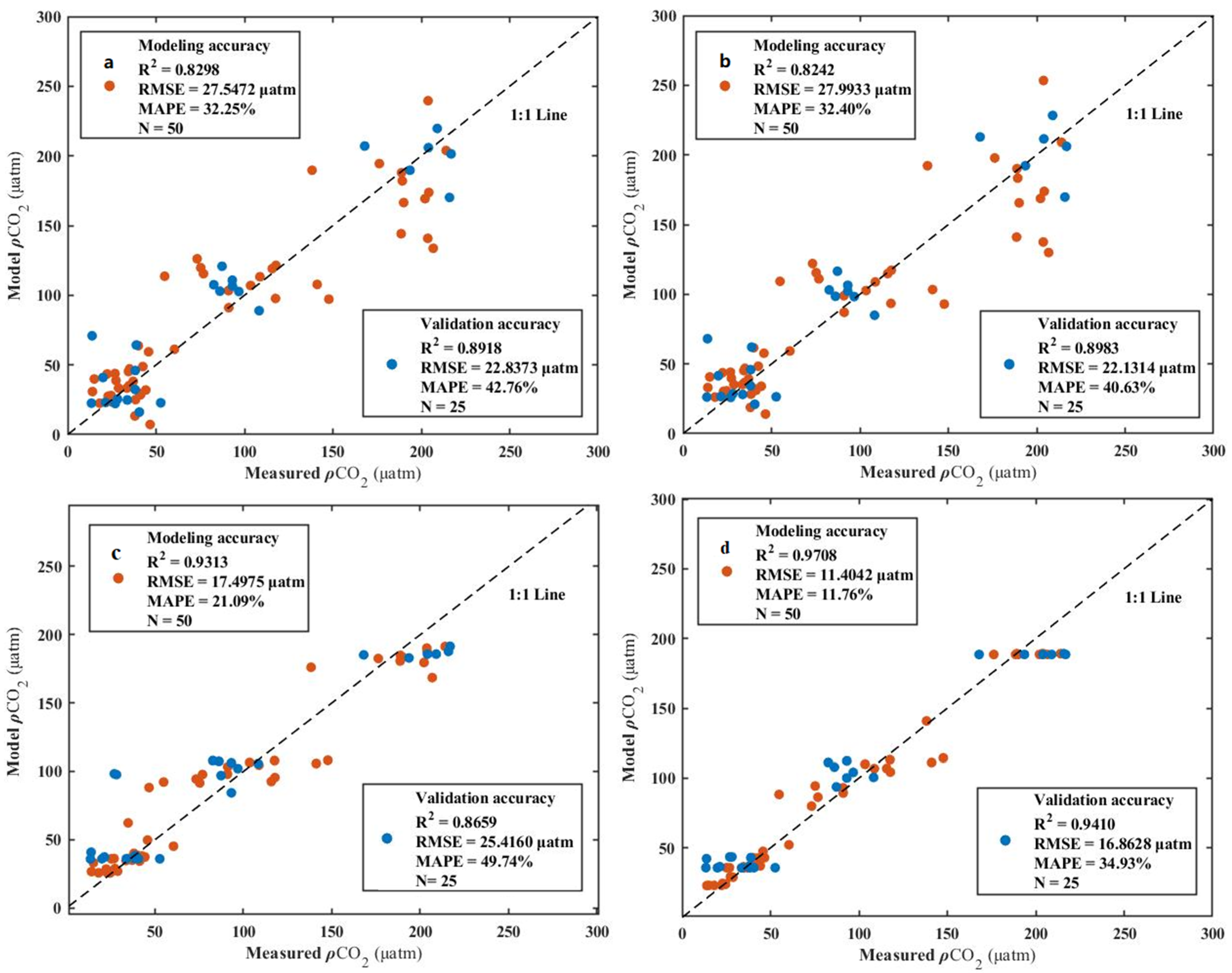
Pure band calculations for regression models inevitably produce negative inversion values in the imagery, which skew the overall results. Nonlinear data are not well fitted. The model was optimized and parameterized using multiple experiments, and the final parameter values are shown in Table 4. Other parameters were assigned default values. Using the same training samples as in the linear model, the random forest and XGBoost pCO2 models were constructed. The pCO2 values predicted by the models vs. those measured in situ are plotted in Figure 2, which reflects the differences between the two types of results for each model. The closer the verification sample points are to the diagonal line, the smaller the model error.
All the tested models from pCO2 collected at 110 sites across Chagan Lake achieved accurate calibration, with R2 ranging from 0.82 to 0.97. Validation results also exhibited stable performance (R2 = 0.87–0.94) (Figure 2). The linear model and band difference model (Figure 2a), i.e., unary one-time models, had R2, RMSE, and MAPE values of 0.83, 27.54 μatm, and 32.25%, respectively. The quadratic model (Figure 2b) showed validation accuracy, with R2, RMSE, and MAPE values of 0.90, 22.13 μatm, and 40.63%, respectively. In general, the accuracy of the linear models was similar and relatively good. The accuracy of the random forest model was high, with R2, RMSE, and MAPE of 0.93, 17.50 μatm, and 21.09% (Figure 2c), respectively, but the validation accuracy was not high, with R2 of 0.87, RMSE of 25.42 μatm, and MAPE of 49.74%. The XGBoost model (Figure 2d) had significantly smaller errors, and its R2, RMSE, and MAPE of 0.97, 11.40 μatm, and 11.76%, respectively, were better than those of other models. The validation accuracy (R2 = 0.94 and RMSE = 16.87 μatm) was also better than those of the remaining three models. The XGBoost model showed the best performance, indicating that it effectively utilized various feature information supporting its nonlinear regression prediction ability.

3.2. Spatiotemporal Analysis of pCO2 Based on the Inversion Results

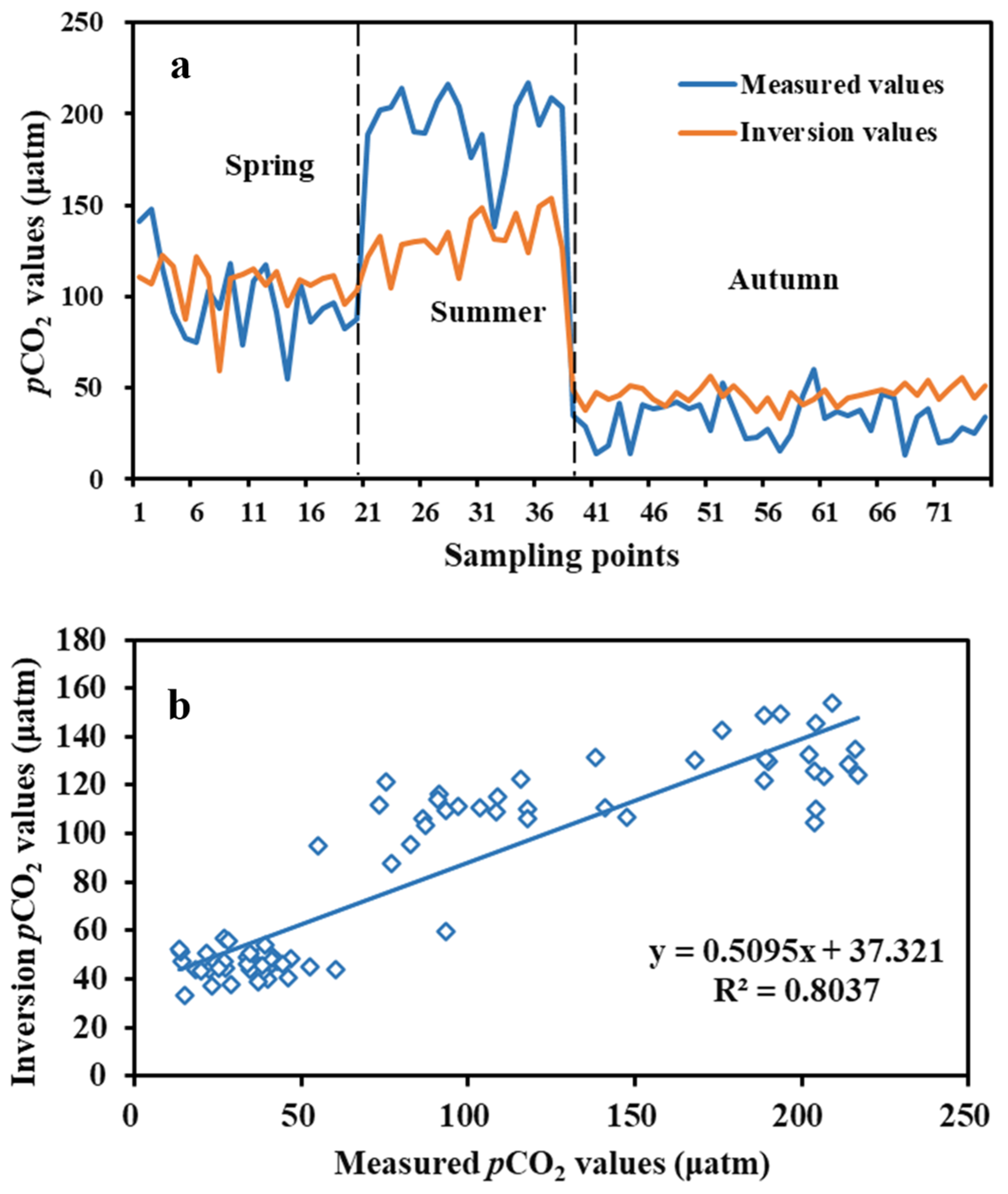
We applied the XGBoost model to map the pCO2 of Chagan Lake in 2021 and obtained satisfactory results (Figure 3). The corresponding inversion result accuracy of the sampling points was also better (R2 = 0.80) (Figure 4). A full-scale assessment of pCO2 in Chagan Lake in 2021 was conducted using the Landsat OLI surface reflectance product in the ice-free season. The pCO2 values of Chagan Lake ranged from 0 to 200 μatm, with 25–75% of them concentrated between 30 and 150 μatm. The minimum value changes were small, concentrated in the range of 15–25 μatm. The spatial distribution of the pCO2 values was higher in the southeast of Chagan Lake than in the northwest. Because of the occurrence of large individual extrema in the models, the maximum and minimum values were not included in the following trend analysis.
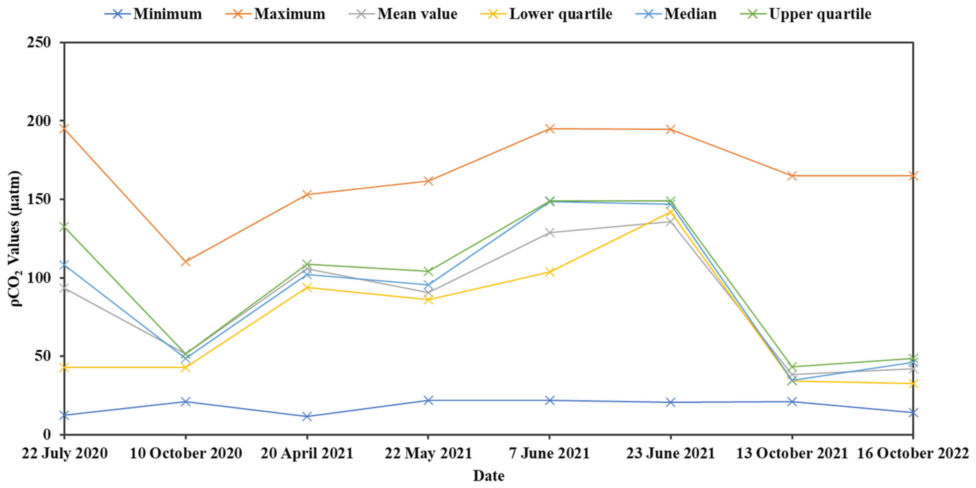
A seasonal analysis of the model results was conducted (Figure 3, spring: March–May; summer: June–August, autumn: September–November). The highest seasonal mean pCO2 values in Chagan Lake were in the summer (mean = 132.45 ± 24.44 μatm), followed by spring (mean = 98.11 ± 18.24 μatm), and the lowest was in autumn (mean = 44.03 ± 8.46 μatm). The characteristic values were analyzed (Figure 5 and Figure 6) and it was revealed that the lowest pCO2 was found in autumn, followed by spring, and highest value was found in summer. The trends of the eigenvalues were essentially consistent (Figure 6a). The mean, lower quartile, median, and upper quartile changes were the highest in summer (120–150 μatm), followed by spring (80–110 μatm) and autumn (30–50 μatm) (Figure 6b). It was observed that the autumn pCO2 values were the lowest; the spring pCO2 values were about twice those of autumn; and the summer pCO2 values were thrice those of autumn and about 1.5 times those of spring. Then, the XGBoost model was used to invert the images and the ENVI Quick Stats function was adopted to obtain the eigenvalues of the inversion results, including the maximum and minimum values; mean; and the lower, median, and upper quartiles, as shown in the Figure 5.
The annual mean pCO2 in Chagan Lake was calculated based on the XGBoost model results. The values significantly increased between 1990 (mean = 42.45 ± 8.50 μatm) and 2021 (mean = 91.52 ± 14.31 μatm) (Figure 7). This trend of annual mean pCO2 was consistent with the increase in nutrient levels in Chagan Lake over the same years. We can see that the values were higher at the boundary of the lake than on the surface in 1990, while in 2021, this was the opposite, as seen in Figure 7. The reason may be that in 2021, the lake biomass of Chagan Lake was large, most of it was concentrated on the lake water surface, and the low biomass at the lake boundary led to low pCO2 values. In the 1980s and 1990s, on the other hand, Chagan Lake was in the process of “introducing loose water into the lake”; the water area was in a period of rapid growth [47]; the development of fishery was slow; there was overfishing; and the overall biomass was small, resulting in high pCO2 values only in the southeast region and low ones overall. The abnormally high value of red in the eastern part of the lake in 1990 was due to the fact that the water area of Chagan Lake was fluctuant between 1990 and 2021. Moreover, we used the same shapefile of Chagan lake, and the boundary of lake may include the transition zone from the lake to the land. In 1990 and 2021, the overall pattern was the same, with the southeast being higher than the northwest.

3.3. CO2 Flux through Water–Atmosphere Interface of Chagan Lake

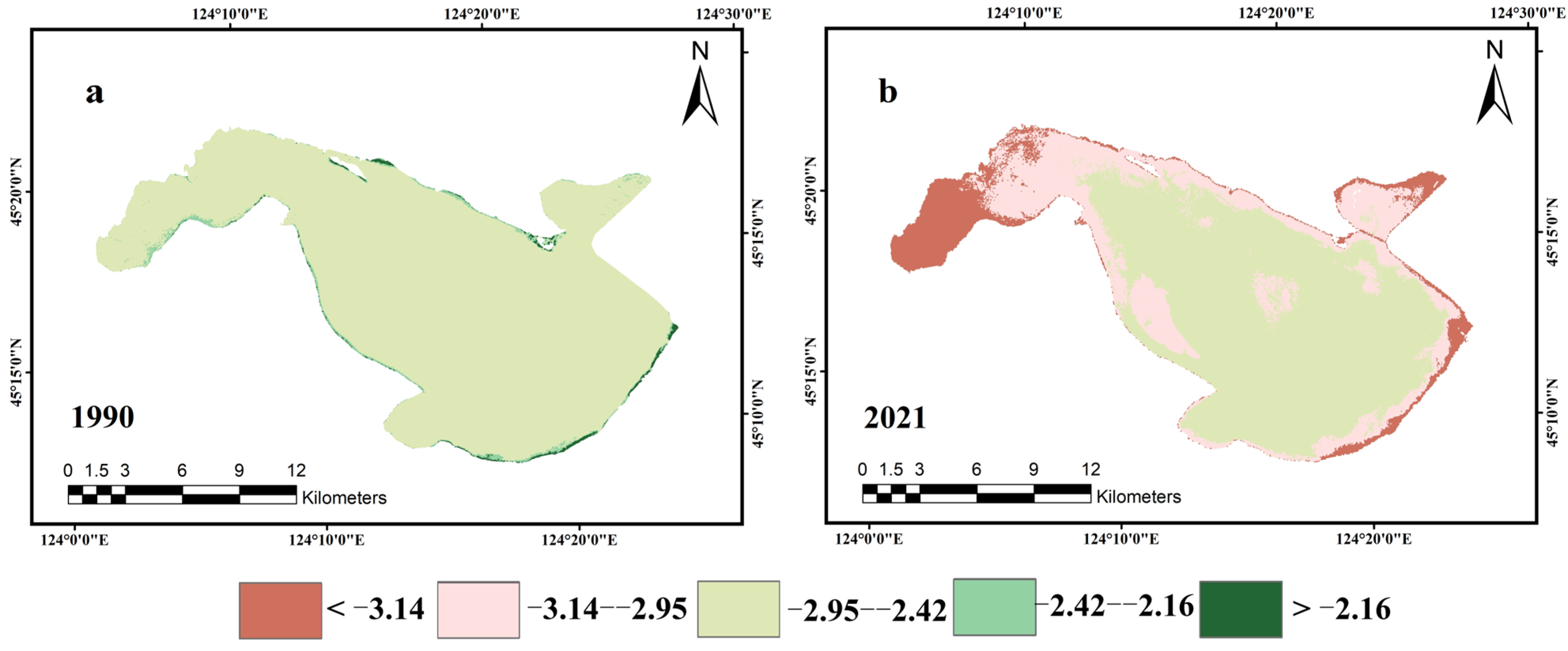
CO2 flux through the water–atmosphere interface of Chagan Lake was calculated based on the modeled pCO2 values. This negative value of CO2 flux values indicates that Chagan Lake was absorbing CO2 from atmosphere (i.e., the lake functioned as a weak carbon sink). The CO2 flux was lowest in summer, ranging between 2.4 and 2.64 mmol/m2/d, followed by spring (2.64–3.12 mmol/m2/d), and it was highest in autumn, with values above 3.36 mmol/m2/d (Figure 8). The study also compared these CO2 fluxes to those in 1990 (Figure 9), which showed that Chagan Lake was a carbon sink in 1990 and 2021 and the CO2 flux increased between 1990 (mean = −2.53 ± 0.07 mmol/m2/d) and 2021 (mean = −2.96 ± 0.13 mmol/m2/d).

3.4. Correlation between pCO2 and Its Influencing Factors

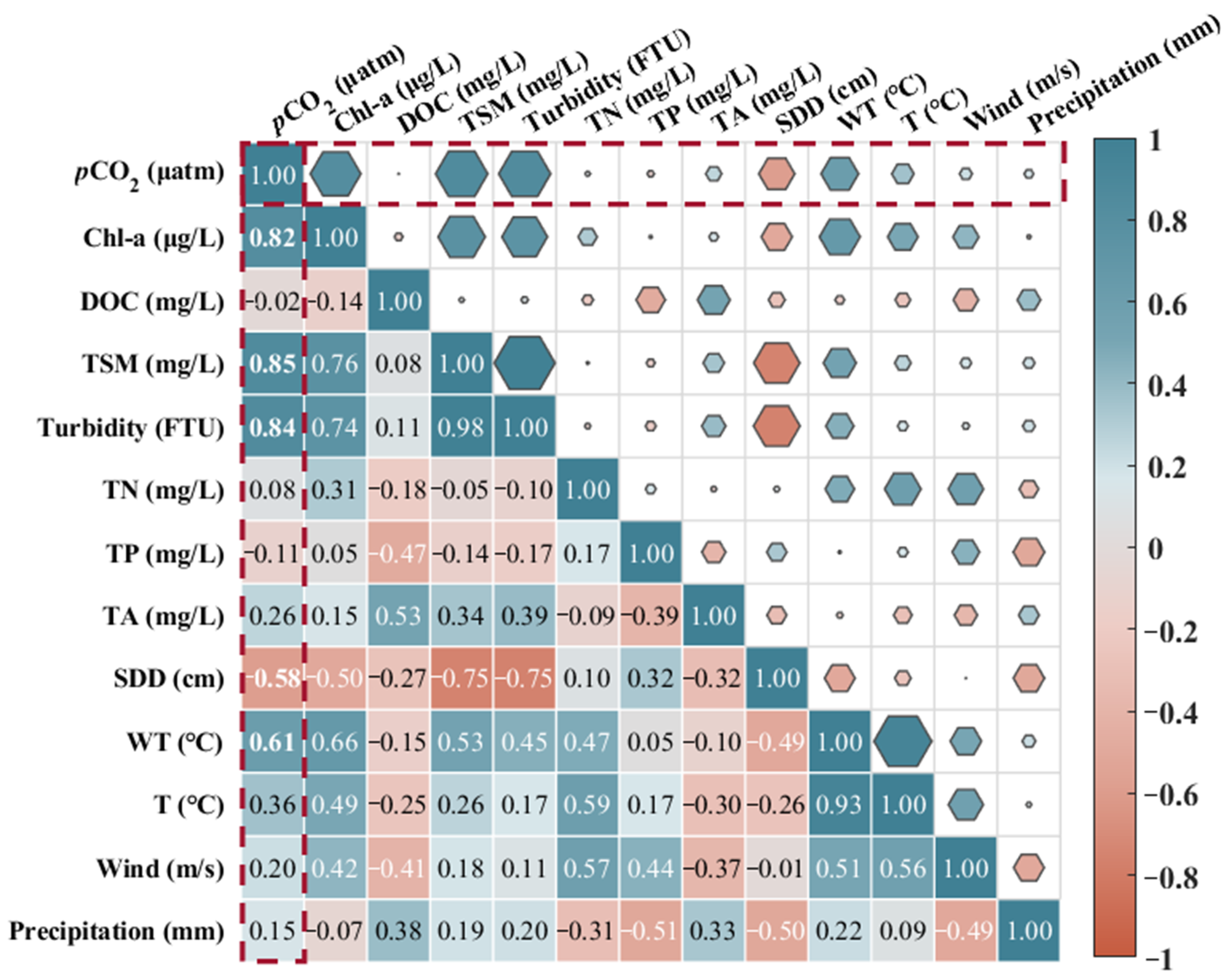
The climatic factors, including temperature, wind speed, and precipitation, were extracted using WRF. The climatic factors were positively correlated with the overall trend of monthly pCO2 with the water temperature showing the highest correlation. However, the relationships between wind speed, precipitation, and pCO2 were not very conclusive (Figure 10). In addition, water quality parameters, chlorophyll a, total suspended solids, and turbidity showed high positive correlations (R2 > 0.8) with the pCO2 values, while the Secchi disk depth (SDD), total nitrogen (TN) and total phosphorus (TP) were all negatively correlated with them. TN varied from 0.74–1.35 mg/L and TP varied from 0.03–0.22 mg/L (Figure 11); this indicates a high degree of eutrophication in the lake.
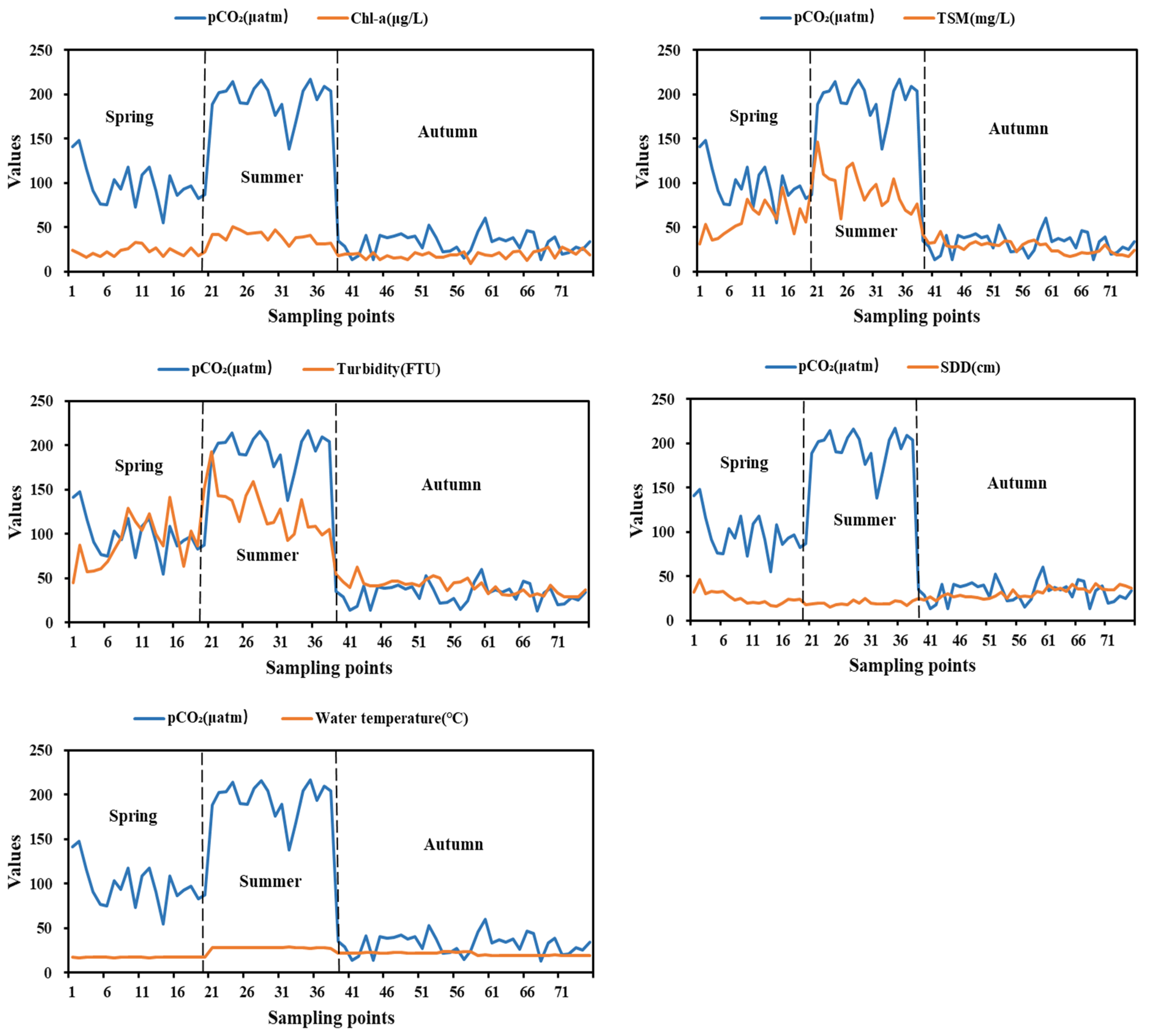
In addition, several influencing factors (chlorophyll a, total suspended solids, turbidity, Secchi disk depth, water temperature) that showed a high correlation with pCO2 were analyzed for their changing trends; these factors mainly presented seasonal fluctuations (Figure 12). Among them, the fluctuations in TSM and turbidity were closest to those of pCO2, with more intense fluctuations, while the changes in chlorophyll and water temperature are relatively gentle, with the values all showing summer > spring > autumn. That is, the values of TSM, turbidity, chlorophyll a, and water temperature are higher in summer, and pCO2 values are also higher, with the lowest values occurring in autumn. The trend of changes in transparency, with autumn > spring > summer, is opposite to pCO2 changes: the lowest transparency is found in summer, while pCO2 is the highest.

4. Discussion

4.1. Temporal and Spatial Variations of pCO2 in Chagan Lake

Because Chagan Lake freezes in the winter, we only studied the seasonal distribution of pCO2 values during the ice-free period of 2021. We found that it exhibited a pattern of high pCO2 values in summer and low ones in autumn (Figure 3), which was similar to the pCO2 value distribution at actual sampling points (Figure 4). This distribution was consistent with the seasonal distributions of the pCO2 values in Beihu Lake and Changchun Park [48], but different from the western part of Chaohu Lake [22] or Taihu Lake [23]. The difference in summer pCO2 values evident in Figure 4 was attributed to the difference between the actual summer sampling time (18 July) and the sampling times of available satellite images (7 June, 23 June and 22 July). Moreover, the measured water temperature, chlorophyll, TSM, and turbidity of Chagan Lake revealed high values in summer and low values in autumn, and their Pearson correlation coefficients with the pCO2 values were 0.61, 0.82, 0.85, and 0.84, respectively (Figure 10). Water temperature is one of the main influencing factors on the horizontal distribution of phytoplankton. Phytoplankton and biomass abundance increase with rising water temperature [49,50], leading to increased photosynthesis and decreased carbon dioxide in lakes. However, in the Chagan Lake wetland, although the water temperature in summer is higher than that in autumn, the number, abundance, and biomass of phytoplankton species are lower than they are in autumn [21,32]. This results in higher pCO2 in summer than in autumn. On the one hand, precipitation increases in summer, and receding water from farmland in the Qianguo irrigation area also flows into Chagan Lake, increasing the water level and diluting phytoplankton and biomass. This leads to a decrease in hydraulic retention time and an increase in water flow speed, significantly affecting the horizontal distribution of phytoplankton [51]. A faster water flow is not conducive to the accumulation of phytoplankton biomass, but simultaneously carries larger amounts of pollutants such as TN and TP, which provide nutrients for phytoplankton growth, manifested as high pigment content [26,50]. On the other hand, as an important fishery industry base in Jilin Province, the Chagan Lake wetland releases hundreds of thousands of catties of fry every spring and autumn. This increases the carbon dioxide concentration in the lake, and as the fish grow, their feed intake also decreases phytoplankton abundance and biomass [50]. This was also visible in the phytoplankton distribution measured at the 2020–2021 sampling points, which was presented by Chang et al. [32].
The pCO2 values in Chagan Lake in 2021 were high in the southeast region and low in the northwest region (Figure 7b). According to the 2020–2021 phytoplankton sampling analysis of Chang et al. [32], the phytoplankton biomass in the southeast of Chagan Lake was essentially smaller than that in the northwest. It comprised mainly chlamydomonas and chlamydomonas ovate, the biomass in summer was lower than in autumn, and photosynthesis absorbed less CO2. This produced a spatial distribution with high pCO2 values in the southeast region and low pCO2 values in the northwest region. Compared to the spatial changes between 1990 and 2021 (Figure 7), the spatial distribution was consistent, but the pCO2 values in 2021 were higher than those in 1990, and the high-value area in southeast China in 2021 was significantly larger than that in 1990, which could be due to the increase in eutrophication in Chagan Lake.

4.2. Chagan Lake as Carbon Source or Sink

In view of the important role and significance of lakes to economic and social development, the ecological environment of lakes has always attracted widespread attention. Since the 18th National Congress of the Communist Party of China, the Party and the state have attached great importance to the cultivation of ecological civilization, and a number of affiliated units have produced five reports. On the basis of these five reports, the Proceedings of the Chinese Academy of Sciences published a series of papers entitled “Progress and Effectiveness of China’s Ecological Civilization Construction”, which scientifically analyzed the long-term ecological environment changes of the aforementioned typical ecosystems and regions, especially the changes since the 18th National Congress of the Communist Party of China, and formulated suggestions for ecological environmental protection [52,53]. From a single treatment measure to a systematic plan for upstream and downstream and left and right bank coordination, the water quality of Chagan Lake has shown a promising trend. The transparency increased from 0.45 m in 2011 to 0.58 m in 2020; the water quality improved from Class V before 2012 to Class IV in 2020; and the fluoride concentration decreased by 13% year-on-year [53]. Chagan Lake has progressed from “no water” to “water” to “clear water”, and the lake area has been stable at 300 km2 since 2012. The concentration of nitrogen and phosphorus in the water has decreased significantly, with mean nitrogen and phosphorus concentrations of 0.949 mg/L and 0.088 mg/L in 2021, respectively (Figure 11).
The analysis of CO2 fluxes conducted in this study showed that Chagan Lake, between 1990 (mean = −2.53 ± 0.07 mmol/m2/d) and 2021 (mean = −2.96 ± 0.13 mmol/m2/d), has been a weak carbon sink. This may be due to the increase in the nutrient content and temperature of lakes in recent years, leading to the vigorous growth of algae and phytoplankton as well as strong photosynthesis, which absorbs and uses large amounts of CO2. Furthermore, the flow rate of lake water was slow, and, in such an environment, photosynthesis consumed more CO2 than the amount of CO2 produced by phytoplankton respiration. Thus, biophotosynthesis was the main factor contributing to the carbon sink state of Chagan Lake [54,55]. As chlorophyll a concentrations increased, the pCO2 values increased too (Figure 10), possibly because phytoplankton is an important primary producer in aquatic ecosystems, with fundamental links to the food chain. However, the rates of increase in CO2 partial pressure in the lake (42.45 ± 8.50 μatm in 1990; 91.52 ± 14.31 μatm in 2021) were lower than the rates of increase in atmospheric CO2 (354.45 ppm in 1990; 416.45 ppm in 2021), keeping Chagan Lake in a carbon sink state. In other words, the degree of eutrophication increased from 1990 to 2021, and the photosynthesis by lake organisms also increased, which in turn promoted carbon dioxide absorption. Eutrophication refers to an abnormal increase in the primary productivity of lake water ecosystems due to excessive intake of nutrients, such as nitrogen and phosphorus, mainly manifested as abnormal reproduction of algae and other plankton [56]. An increase in primary productivity means that water ecosystems fix more CO2, which in turn reduces CO2 emissions [22,57].
In addition, in Chagan Lake, the correlations between total suspended matter concentration and turbidity and pCO2 were high (Figure 10). High turbidity increases the respiration rate of aquatic animals and plants and promotes CO2 production and release [58]. SDD is negatively correlated with pCO2, and with decreasing SDD, CO2 emissions fall and the degree of eutrophication increases.
Among the meteorological factors influencing pCO2, temperature (R2 = 0.36) was the strongest, wind speed (R2 = 0.20) came second, and precipitation (R2 = 0.15) third, all positively correlated with pCO2 (Figure 10). However, none of these were dominant factors. When cool lakes warm up due to seasonal or long-term climate changes, they may begin to emit more CO2 [37]. Wind speed can affect the water–CO2 flux of CO2 by affecting the gas transport coefficient, the decomposition of carbon matter in water, and the production of carbon dioxide [54,59]. Precipitation affects exogenous inputs, such as rivers that carry substantial amounts of organic matter and inorganic carbon into lakes, promoting CO2 emissions [60].

4.3. Uncertainty Analysis

In this paper, a spatiotemporal analysis of the partial pressures and emission fluxes of CO2 in Chagan Lake was conducted and the factors affecting CO2 emissions in Chagan Lake were discussed, which provided reference values for studying the contribution of inland lakes to global GHG emissions. However, with the limited measured data available, this study still requires several improvements, as follows:
(1)
Although the lake water samples we collected met the basic requirements (including water sample collection depth (0.1–0.5 m), water sample storage temperature (4 °C), etc.), due to the limitations of time and in situ sampling conditions, the number of samples acquired was only modest. This might have had an impact on the accuracy of the models we subsequently constructed using the in situ data. Thus, we will endeavor to collect more in situ samples to improve our models and the accuracy of their predictions.
(2)
Because the time span of our data was small, it needs to be increased. Also, the influence of wind speed on CO2 needs to be more accurately assessed in the analysis of climate impact factors.

5. Conclusions

This study used Landsat 8 satellite images to monitor the pCO2 and CO2 flux changes in Chagan Lake. A comparison of the predictive performance of a linear regression model and a machine learning model revealed that the XGBoost model had the highest fitting accuracy (R2 = 0.94, RMSE = 16.86 μatm), and hence was used to map the pCO2 variation in Chagan Lake in 2021. The pCO2 in the surface water of Chagan Lake showed a considerable spatial variability within a range of 0–200 μatm during the ice-free period. In terms of seasonal variation, the highest values were found in the summer, followed by spring and autumn. The CO2 fluxes calculated from the pCO2 values ranged from −3.69 to −2.42 mmol/m2/d, which indicates that Chagan Lake was absorbing CO2 (i.e., it was a weak carbon sink). Increasing temperature drove the increase in pCO2, and CO2 emissions in Chagan Lake, along with the deterioration of the trophic states. Based on the results of this study, actively carrying out eutrophication management, reducing the degree of eutrophication in lakes, and maintaining the reasonable development of fisheries can make important contributions to reducing carbon dioxide emissions in lakes and strengthening the carbon sink function of lakes. The results of this study provide important data and insights needed to implement effective practices for the regulation of the carbon cycle in lakes.

Author Contributions

Conceptualization: R.Z. and Z.W.; methodology: R.Z. and G.L.; software: Q.Y.; validation: C.F.; formal analysis: Y.S.; investigation: Q.Y., S.L. and H.T.; data curation: L.L. and K.S.; writing—original draft preparation: R.Z.; writing—review and editing: Z.W.; visualization and supervision: K.S.; funding acquisition: Z.W., S.L., Y.S., G.L. and K.S. All authors have read and agreed to the published version of the manuscript.

Funding

This research was jointly supported by the Natural Science Foundation of Jilin Province, China (20220203024SF) Zhidan Wen; the National Natural Science Foundation of China (U2243230, 42371390, 42171385, 42201414), Kaishan Song, Yingxin Shang, Ge Liu, Sijia Li; Youth Innovation Promotion Association of Chinese Academy of Sciences, China (2020234) Zhidan Wen; Young Scientist Group Project of Northeast Institute of Geography and Agroecology, Chinese Academy of Sciences (2023QNXZ01) Zhidan Wen; Land Observation Satellite Supporting Platform of National Civil Space Infrastructure Project (CASPLOS-CCSI) Sijia Li, and Postdoctoral Fellowship of Jilin Province of China to Yingxin Shang.

Data Availability Statement

Data are contained within the article.

Acknowledgments

Thanks to USGS and GEE for the Landsat data. Thanks to the NCAR Research Data Archive (RDA) for the FNL data. We also acknowledge the data support from National Climatic Data Center of the National Oceanic and Atmospheric Administration and the Global Monitoring Laboratory (GML) of the National Oceanic and Atmospheric Administration.

Conflicts of Interest

The authors declare no conflict of interest.

References

  1. Ballantyne, A.P.; Alden, C.B.; Miller, J.B.; Tans, P.P.; White, J.W.C. Increase in observed net carbon dioxide uptake by land and oceans during the past 50 years. Nature 2012, 488, 70–72. [Google Scholar] [CrossRef]
  2. IPCC. Climate Change 2021: The Physical Science Basis. Contribution of Working Group I to the Sixth Assessment Report of the Intergovernmental Panel on Climate Change; Cambridge University Press: Cambridge, UK; New York, NY, USA, 2021; Volume In Press. [Google Scholar]
  3. Barral, A.; Gomez, B.; Fourel, F.; Daviero-Gomez, V.; Lécuyer, C. CO2 and temperature decoupling at the million-year scale during the Cretaceous Greenhouse. Sci. Rep. 2017, 7, 8310. [Google Scholar] [CrossRef]
  4. Davidson, E.A.; Suddick, E.C.; Rice, C.W.; Prokopy, L.S. More Food, Low Pollution (Mo Fo Lo Po): A Grand Challenge for the 21st Century. J. Environ. Qual. 2015, 44, 305–311. [Google Scholar] [CrossRef] [PubMed]
  5. Linquist, B.A.; Anders, M.M.; Adviento-Borbe, M.A.A.; Chaney, R.L.; Nalley, L.L.; da Rosa, E.F.F.; van Kessel, C. Reducing greenhouse gas emissions, water use, and grain arsenic levels in rice systems. Glob. Chang. Biol. 2014, 21, 407–417. [Google Scholar] [CrossRef]
  6. Yao, Z.; Zheng, X.; Liu, C.; Lin, S.; Zuo, Q.; Butterbach-Bahl, K. Improving rice production sustainability by reducing water demand and greenhouse gas emissions with biodegradable films. Sci. Rep. 2017, 7, 39855. [Google Scholar] [CrossRef] [PubMed]
  7. Weyhenmeyer, G.A.; Kosten, S.; Wallin, M.B.; Tranvik, L.J.; Jeppesen, E.; Roland, F. Significant fraction of CO2 emissions from boreal lakes derived from hydrologic inorganic carbon inputs. Nat. Geosci. 2015, 8, 933–936. [Google Scholar] [CrossRef]
  8. Verpoorter, C.; Kutser, T.; Seekell, D.A.; Tranvik, L.J. A global inventory of lakes based on high-resolution satellite imagery. Geophys. Res. Lett. 2014, 41, 6396–6402. [Google Scholar] [CrossRef]
  9. Raymond, P.A.; Hartmann, J.; Lauerwald, R.; Sobek, S.; McDonald, C.; Hoover, M.; Butman, D.; Striegl, R.; Mayorga, E.; Humborg, C.; et al. Global carbon dioxide emissions from inland waters. Nature 2013, 503, 355–359. [Google Scholar] [CrossRef] [PubMed]
  10. Borges, A.V.; Darchambeau, F.; Teodoru, C.R.; Marwick, T.R.; Tamooh, F.; Geeraert, N.; Omengo, F.O.; Guérin, F.; Lambert, T.; Morana, C.; et al. Globally significant greenhouse-gas emissions from African inland waters. Nat. Geosci. 2015, 8, 637–642. [Google Scholar] [CrossRef]
  11. Wen, Z.; Shang, Y.; Lyu, L.; Li, S.; Tao, H.; Song, K. A Review of Quantifying pCO2 in Inland Waters with a Global Perspective: Challenges and Prospects of Implementing Remote Sensing Technology. Remote Sens. 2021, 13, 4916. [Google Scholar] [CrossRef]
  12. Ciais, P.; Chris, S.; Govindasamy, B.; Bopp, L.; Brovkin, V.; Canadell, J.; Chhabra, A.; Defries, R.; Galloway, J.; Heimann, M. Carbon and other biogeochemical cycles. In Climate Change 2013: The Physical Science Basis; Cambridge University Press: Cambridge, UK, 2013; pp. 465–570. [Google Scholar]
  13. Kutser, T.; Verpoorter, C.; Paavel, B.; Tranvik, L.J. Estimating lake carbon fractions from remote sensing data. Remote Sens. Environ. 2015, 157, 138–146. [Google Scholar] [CrossRef]
  14. Cole, J.J.; Prairie, Y.T.; Caraco, N.F.; McDowell, W.H.; Tranvik, L.J.; Striegl, R.G.; Duarte, C.M.; Kortelainen, P.; Downing, J.A.; Middelburg, J.J.; et al. Plumbing the Global Carbon Cycle: Integrating Inland Waters into the Terrestrial Carbon Budget. Ecosystems 2007, 10, 172–185. [Google Scholar] [CrossRef]
  15. Holgerson, M.A.; Raymond, P.A. Large contribution to inland water CO2 and CH4 emissions from very small ponds. Nat. Geosci. 2016, 9, 222–226. [Google Scholar] [CrossRef]
  16. Luo, X.; Croft, H.; Chen, J.M.; He, L.; Keenan, T.F. Improved estimates of global terrestrial photosynthesis using information on leaf chlorophyll content. Glob. Chang. Biol. 2019, 25, 2499–2514. [Google Scholar] [CrossRef] [PubMed]
  17. Xiao, Q.; Xu, X.; Duan, H.; Qi, T.; Qin, B.; Lee, X.; Hu, Z.; Wang, W.; Xiao, W.; Zhang, M. Eutrophic Lake Taihu as a significant CO2 source during 2000–2015. Water Res. 2020, 170, 115331. [Google Scholar] [CrossRef] [PubMed]
  18. Huotari, J.; Ojala, A.; Peltomaa, E.; Nordbo, A.; Launiainen, S.; Pumpanen, J.; Rasilo, T.; Hari, P.; Vesala, T. Long-term direct CO2 flux measurements over a boreal lake: Five years of eddy covariance data. Geophys. Res. Lett. 2011, 38, L18401. [Google Scholar] [CrossRef]
  19. Reed, D.E.; Dugan, H.A.; Flannery, A.L.; Desai, A.R. Carbon sink and source dynamics of a eutrophic deep lake using multiple flux observations over multiple years. Limnol. Oceanogr. Lett. 2018, 3, 285–292. [Google Scholar] [CrossRef]
  20. Kling, G.W.; Kipphut, G.W.; Miller, M.C. The flux of CO2 and CH4 from lakes and rivers in arctic Alaska. Hydrobiologia 1992, 240, 23–36. [Google Scholar] [CrossRef]
  21. Zhao, M.; Jiao, S.; Liang, H.; Cao, Y.; Zhao, Z.; Zhang, Q.; Yuan, R. Temporal and spatial variation of carbon dioxide partial pressure and exchange flux characteristics in the backwater area of Wanfeng Lake Reservoir. Environ. Chem. 2019, 38, 1307–1317. [Google Scholar] [CrossRef]
  22. Tianci, Q.I.; Qitao, X.; Yuqing, M.; Hongtao, D. Temporal and spatial variation of carbon dioxide concentration and its exchange fluxes in Lake Chaohu. J. Lake Sci. 2019, 31, 766–778. [Google Scholar] [CrossRef]
  23. Qi, T.; Xiao, Q.; Cao, Z.; Shen, M.; Ma, J.; Liu, D.; Duan, H. Satellite Estimation of Dissolved Carbon Dioxide Concentrations in China’s Lake Taihu. Environ. Sci. Technol. 2020, 54, 13709–13718. [Google Scholar] [CrossRef] [PubMed]
  24. Zhang, B.; Li, J.; Shen, Q.; Wu, Y.; Zhang, F.; Wang, S.; Yao, Y.; Guo, L.; Yin, Z. Recent research progress on long time series and large scale optical remote sensing of inland water. Natl. Remote Sens. Bull. 2021, 25, 37–52. [Google Scholar] [CrossRef]
  25. Song, K.; Liu, G.; Wang, Q.; Wen, Z.; Lyu, L.; Du, Y.; Sha, L.; Fang, C. Quantification of lake clarity in China using Landsat OLI imagery data. Remote Sens. Environ. 2020, 243, 111800. [Google Scholar] [CrossRef]
  26. Wang, J.; Zhao, Q.; Pang, Y.; Hu, K. Research on nutrient pollution load in Lake Taihu, China. Environ. Sci. Pollut. Res. 2017, 24, 17829–17838. [Google Scholar] [CrossRef] [PubMed]
  27. Shi, K.; Zhang, Y.; Zhou, Y.; Liu, X.; Zhu, G.; Qin, B.; Gao, G. Long-term MODIS observations of cyanobacterial dynamics in Lake Taihu: Responses to nutrient enrichment and meteorological factors. Sci. Rep. 2017, 7, 40326. [Google Scholar] [CrossRef] [PubMed]
  28. Yin, Z.; Li, J.; Zhang, B.; Liu, Y.; Yan, K.; Gao, M.; Xie, Y.; Zhang, F.; Wang, S. Increase in chlorophyll-a concentration in Lake Taihu from 1984 to 2021 based on Landsat observations. Sci. Total Environ. 2023, 873, 162168. [Google Scholar] [CrossRef]
  29. Xie, C.; Zhang, X.; Zhuang, L.; Zhu, R.; Guo, J. Analysis of surface temperature variation of lakes in China using MODIS land surface temperature data. Sci. Rep. 2022, 12, 2415. [Google Scholar] [CrossRef]
  30. Sagan, V.; Peterson, K.; Maimaitijiang, M.; Sidike, P.; Sloan, J.; Greeling, B.; Maalouf, S.; Adams, C. Monitoring inland water quality using remote sensing: Potential and limitations of spectral indices, bio-optical simulations, machine learning, and cloud computing. Earth-Sci. Rev. 2020, 205, 103187. [Google Scholar] [CrossRef]
  31. Yao, L.; Zhao, X.; Zhou, G.-J.; Liang, R.; Gou, T.; Xia, B.; Li, S.; Liu, C. Seasonal Succession of Phytoplankton Functional Groups and Driving Factors of Cyanobacterial Blooms in a Subtropical Reservoir in South China. Water 2020, 12, 1167. [Google Scholar] [CrossRef]
  32. Chang, C.; Wang, Y.; Zhao, C.; Liu, Z.; Ma, C. Seasonal succession of phytoplankton functional groups in Chagan Lake and its influencing factors. Chin. J. Ecol. 2023, 1–9. Available online: https://link.cnki.net/urlid/21.1148.Q.20230510.1734.005 (accessed on 6 December 2023).
  33. Liu, X.; Zhang, G.; Sun, G.; Wu, Y.; Chen, Y. Assessment of Lake Water Quality and Eutrophication Risk in an Agricultural Irrigation Area: A Case Study of the Chagan Lake in Northeast China. Water 2019, 11, 2380. [Google Scholar] [CrossRef]
  34. Schindler, D.W.; Carpenter, S.R.; Chapra, S.C.; Hecky, R.E.; Orihel, D.M. Reducing Phosphorus to Curb Lake Eutrophication is a Success. Environ. Sci. Technol. 2016, 50, 8923–8929. [Google Scholar] [CrossRef] [PubMed]
  35. Cole, J.J.; Caraco, N.F.; Kling, G.W.; Kratz, T.K. Carbon Dioxide Supersaturation in the Surface Waters of Lakes. Science 1994, 265, 1568–1570. [Google Scholar] [CrossRef] [PubMed]
  36. Lundin, E.J.; Giesler, R.; Persson, A.; Thompson, M.S.; Karlsson, J. Integrating carbon emissions from lakes and streams in a subarctic catchment. Geophys. Res. Biogeosci. 2013, 118, 1200–1207. [Google Scholar] [CrossRef]
  37. Wen, Z.; Song, K.; Shang, Y.; Fang, C.; Li, L.; Lv, L.; Lv, X.; Chen, L. Carbon dioxide emissions from lakes and reservoirs of China: A regional estimate based on the calculated pCO2. Atmos. Environ. 2017, 170, 71–81. [Google Scholar] [CrossRef]
  38. Ma, J. Inversion of Kd(PAR) and Euphotic Zone Depth of Typical Water Bodys in Northeast China with Remote Imagery. Master’s Thesis, University of Chinese Academy of Sicences, Shenzhen, China, 2017. [Google Scholar]
  39. Haddout, S.; Priya, K.L.; Hoguane, A.M.; Casila, J.C.C.; Ljubenkov, I. Relationship of salinity, temperature, pH, and transparency to dissolved oxygen in the Bouregreg estuary (Morocco): First results. Water Pract. Technol. 2022, 17, 2654–2663. [Google Scholar] [CrossRef]
  40. Roy, D.P.; Kovalskyy, V.; Zhang, H.K.; Vermote, E.F.; Yan, L.; Kumar, S.S.; Egorov, A. Characterization of Landsat-7 to Landsat-8 reflective wavelength and normalized difference vegetation index continuity. Remote Sens. Environ. 2016, 185, 57–70. [Google Scholar] [CrossRef]
  41. Teodoru, C.R.; del Giorgio, P.A.; Prairie, Y.T.; Camire, M. Patterns in pCO2 in boreal streams and rivers of northern Quebec Canada. Glob. Biogeochem. Cycles 2009, 23, GB2012. [Google Scholar] [CrossRef]
  42. Cole, J.; Caracao, N. Carbon in catchments: Connecting terrestrial carbon losses with aquatic metabolism. Mar. Freshw. Res. 2001, 52, 101–110. [Google Scholar] [CrossRef]
  43. Cole, J.J.; Caraco, N.F. Atmospheric exchange of carbon dioxide in a low-wind oligotrophic lake measured by the addition of SF6. Limnol. Oceanogr. 1998, 43, 647–656. [Google Scholar] [CrossRef]
  44. Crusius, J.; Wanninkhof, R. Gas transfer velocities measured at low wind speed over a lake. Limnol. Oceanogr. 2003, 48, 1010–1017. [Google Scholar] [CrossRef]
  45. Wanninkhof, R. Relationship between wind speed and gas exchange over the ocean. J. Geophys. Res. Ocean. 1992, 97, 7373–7382. [Google Scholar] [CrossRef]
  46. Li, S.; Bush, R.T.; Santos, I.R.; Zhang, Q.; Song, K.; Mao, R.; Wen, Z.; Lu, X.X. Large greenhouse gases emissions from China’s lakes and reservoirs. Water Res. 2018, 147, 13–24. [Google Scholar] [CrossRef]
  47. Fang, H.; He, Z.; Chen, X.; Tian, X. Spatial-temporal change of Chagan Lake and response to precipitation change from 1985 to 2018. China Agric. Inform. 2020, 32, 64–73. [Google Scholar] [CrossRef]
  48. Wen, Z.; Song, K.; Zhao, Y.; Shao, T.; Li, S. Seasonal Variability of Greenhouse Gas Emissions in the Urban Lakes in Changchun, China. Huanjing Kexue 2016, 37, 102–111. [Google Scholar] [CrossRef] [PubMed]
  49. Lehman, P.W. The influence of climate on phytoplankton community biomass in San Francisco Bay Estuary. Limnol. Oceanogr. 2000, 45, 580–590. [Google Scholar] [CrossRef]
  50. Li, R.; Zhang, G.; Zhang, L. Multivariate analysis of the relations between phytoplankton assemblages and environmental factors in Chagan Lake Wetland. Acta Ecol. Sin. 2014, 34, 2663–2673. [Google Scholar] [CrossRef]
  51. Wu, N.; Tang, T.; Zhou, S.; Fu, X.; Jiang, W.; Li, F.; Cai, Q. Influence of cascaded exploitation of small hydropower on phytoplankton in Xiangxi River. J. Appl. Ecol. 2007, 18, 1091–1096. [Google Scholar]
  52. Zhang, Y.; Qin, B.; Zhu, G.; Song, C.; Deng, J.; Xue, B.; Gong, Z.; Wang, X.; Wu, J.; Shi, K.; et al. Importance and main ecological and environmental problems of lakes in China. Chin. Sci. Bull. 2022, 67, 3503–3519. [Google Scholar] [CrossRef]
  53. Zhang, G.; Gu, X.; Zhao, T.; Zhang, Y.; Xu, L. Ecological and Environmental Changes and Protection Measures of Lakes in China. Bull. Chin. Acad. Sci. 2023, 38, 358–364. [Google Scholar] [CrossRef]
  54. Luo, J.C.; Ni, M.F.; Li, S.Y. Water-Air Interface CO2 Exchange Flux of Typical Lakes in a Mountainous Area of the Western Chongqing and Their Influencing Factors. Huanjing Kexue 2019, 40, 192–199. [Google Scholar] [CrossRef]
  55. Wang, J.; Zhou, Y.; Zhou, L.; Zhang, Y.; Qin, B.; Spencer, R.G.M.; Brookes, J.D.; Jeppesen, E.; Weyhenmeyer, G.A.; Wu, F. Urbanization in developing countries overrides catchment productivity in fueling inland water CO2 emissions. Glob. Chang. Biol. 2023, 29, 1–4. [Google Scholar] [CrossRef] [PubMed]
  56. Xi, S. The Distribution, Environmental Impacts and Preventation Contermeasures of Nitrogen and Phosphate in the Chaohu Lake. Doctoral Dissertation, University of Science and Technology of China, Hefei, China, 2016. [Google Scholar]
  57. Pacheco, F.; Roland, F.; Downing, J. Eutrophication reverses whole-lake carbon budgets. Inland Waters 2014, 4, 41–48. [Google Scholar] [CrossRef]
  58. Shen, X.; Sun, T.; Su, M.; Dang, Z.; Yang, Z. Short-term response of aquatic ecosystem metabolism to turbidity disturbance in experimental estuarine wetlands. Ecol. Eng. 2019, 136, 55–61. [Google Scholar] [CrossRef]
  59. Jiang, T.; Guo, J.; Li, Z.; Fang, F.; Bai, L.; Jing, L. Air-water surface greenhouse gas flux in Pengxi river at different operational stages of the Three Gorges Reservoir. Huanjing Kexue 2012, 33, 1463–1470. [Google Scholar]
  60. Junyu, Z.; Kai, P.; Yuyang, L.; Chaorong, L.; Lei, Z.; Yongqiang, Z.; Yanqing, D. Characteristics and influence factors of carbon dioxide efflux from Lake Hongze under different hydrological scenarios. J. Lake Sci. 2022, 34, 1347–1358. [Google Scholar] [CrossRef]
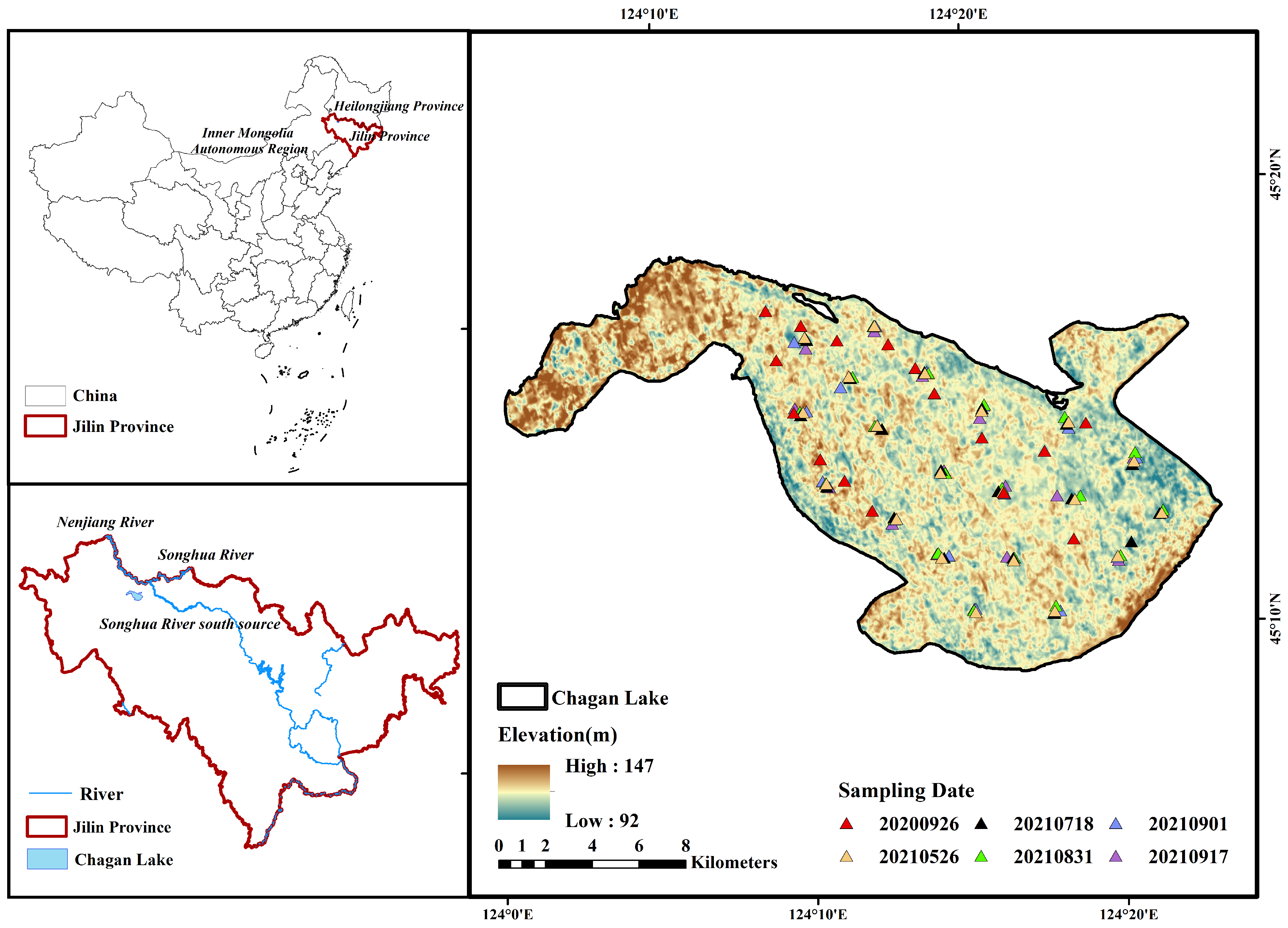
Figure 1. Locations of sampling sites in Chagan Lake.
Remotesensing 15 05680 g001
Figure 2. Calibration and validation of pCO2 model for Chagan Lake based on band surface reflectance. (a) Band difference regression model; (b) exponential regression model; (c) random forest model; (d) XGBoost model.
Remotesensing 15 05680 g002
Figure 3. pCO2 variation in different seasons in 2021 based on inversion values. (a) Spring; (b) summer; (c) autumn. Unit: μatm.
Remotesensing 15 05680 g003
Figure 4. Quarterly comparison and precision of measured pCO2 and inversion values at sampling points. (a) Quarterly comparison of measured pCO2 and inversion values at sampling points; (b) Precision of measured pCO2 and inversion values at sampling points.
Remotesensing 15 05680 g004
Figure 5. Monthly series variation analysis of pCO2 eigenvalues.
Remotesensing 15 05680 g005
Figure 6. Quarterly series variation analysis of pCO2 eigenvalues. (a) The variation of pCO2 eigenvalues with quarter; (b) Comparison of the variation trend of pCO2 eigenvalues in each quater.
Remotesensing 15 05680 g006
Figure 7. Variations in annual mean pCO2 values in 1990 and 2021. (a) 1990; (b) 2021. Unit: μatm.
Remotesensing 15 05680 g007
Figure 8. CO2 flux variation in different seasons, calculated from the inversion pCO2 value. (a) Spring; (b) summer; (c) autumn. Unit: mmol/m2/d.
Remotesensing 15 05680 g008
Figure 9. Variations in annual mean CO2 fluxes in 1990 and 2021. (a) 1990; (b) 2021. Unit: mmol/m2/d.
Remotesensing 15 05680 g009
Figure 10. Relationship between pCO2 values and influencing factors. TN: total nitrogen concentration; TP: total phosphorus concentration; TA: total alkalinity concentration; WT: water temperature; T: air temperature; SDD: Secchi disk depth.
Remotesensing 15 05680 g010
Figure 11. Measured nitrogen and phosphorus concentration at the sampling points.
Remotesensing 15 05680 g011
Figure 12. The change trend of influencing factors and pCO2.
Remotesensing 15 05680 g012
Table 1. The date and quantity of images downloaded.
ImageDateResolutionCloud Cover
LC08_119029_2020072222 July 202030 m<5%
LC08_119029_2020101010 October 202030 m<5%
LC08_119029_2021042020 April 202130 m<5%
LC08_119029_2021052222 May 202130 m<5%
LC08_119029_202106077 June 202130 m<5%
LC08_119029_2021062323 June 202130 m<20%
LC08_119029_202107099 July 202130 m-
LC08_120028_202109022 September 202130 m-
LC08_119029_2021091111 September 2021 30 m-
LC08_119029_2021101313 October 202130 m<5%
LC08_119029_2022101616 October 202230 m<5%
LT05_119029_198908022 August 198930 m<20%
LT05_119029_1989102121 October 198930 m<5%
LT05_119029_199007044 July 199030 m<20%
LT05_119029_199009066 September 199030 m<5%
LT05_119029_1990102424 October 199030 m<5%
LT05_119029_1991041818 April 199130 m<5%
LT05_119029_199105044 May 199130 m<5%
LT05_119029_199106055 June 199130 m<5%
LT05_119029_1991082424 August 199130 m<20%
LT05_119029_199109099 September 199130 m<5%
LT05_119029_1991102727 October 199130 m<5%
Table 2. Pearson correlation coefficient (p) between pCO2 and bands of Landsat 8 images.
FactorsB1B2B3B4B5B6B7
p−0.252−0.1680.182−0.048−0.3820.0460.228
FactorsB3 − B2B5 − B3B5 − B4B4 − B3exp(B3) − exp(B5))/
(exp(B3) + exp(B5)
(B5 − B2)/
(B5 + B2)
p0.703−0.911−0.636−0.600−0.910−0.621
Table 3. Regression models.
Regression ModelFormulaR2
Band difference modely = −4639.749 × (B5 − B3) − 353.8450.83
y = 3824.755 × (B3 − B2) − 109.7210.48
y = −3976.502 × (B5 − B4) + 157.2290.39
Band ratio modely = −93.365 × ((B5 − B2)/(B5 + B2)) + 22.6690.37
y = −156.216 × ((B5-B2)/(B5 + B2)) + 1928.883 × ((B3 + B4)/2) − 214.6380.67
Exponential modely = 93273.487 × (exp(B3) − exp(B5))2/(exp(B3) + exp(B5))2 − 127.0660.82
Table 4. Important model parameter values.
Random Forest ParametersValuesXGBoost ParametersValues
n_estimators80n_estimators50
random_state110learning_rate0.11
max_featuressqrtboostergbtree
max_depth5max_depth5
min_samples_leaf3gamma2
n_jobs−1lambda7
Disclaimer/Publisher’s Note: The statements, opinions and data contained in all publications are solely those of the individual author(s) and contributor(s) and not of MDPI and/or the editor(s). MDPI and/or the editor(s) disclaim responsibility for any injury to people or property resulting from any ideas, methods, instructions or products referred to in the content.