Abstract
The monitoring of crop phenology informs decisions in environmental and agricultural management at both global and farm scales. Current methodologies for crop monitoring using remote sensing data track crop growth stages over time based on single, scalar vegetative indices (e.g., NDVI). Crop growth and senescence are indistinguishable when using scalar indices without additional information (e.g., planting date). By using a pair of normalized difference (ND) metrics derived from hyperspectral data—one primarily sensitive to chlorophyll concentration and the other primarily sensitive to water content—it is possible to track crop characteristics based on the spectral changes only. In a two-dimensional plot of the metrics (ND-space), bare soil, full canopy, and senesced vegetation data all plot in separate, distinct locations regardless of the year. The path traced in the ND-space over the growing season repeats from year to year, with variations that can be related to weather patterns. Senescence follows a return path that is distinct from the growth path.
1. Introduction
Crop phenology, the physiological stages of crop growth and development from planting to harvest, is impacted by genetics, environment, and the management practices imposed on a crop [1]. Accurate monitoring of crop phenology throughout the crop growing season can serve multiple purposes at both global and farm scales. It can be a good indicator of large-scale trends, such as carbon, water, and energy fluxes, and can also provide key information at the farm scale, dictating the timing of several crop management interventions [2,3,4]. Remote sensing data appear to be well adapted to the large-scale, near-real-time monitoring of crop phenology when supported by field observations and the modeling [5] of a plant’s physiological stages. However, current methodology for measuring crop phenology with remote sensing based on scalar vegetation indices limits the potential of this approach. This study explores the potential of the newly defined ND-space to better track crop phenology [6].
1.1. Crop Phenology: Importance from the Farm Level to the Global Level
Crop phenology monitoring is a valuable tool at the global scale for producing national crop production forecasts and allowing private sectors and countries to better prepare for over- or under-production of food, feed, fiber, and fuel [7,8]. It is also an effective way to closely monitor the impacts of weather extremes and climate change in space and time, allowing for a better understanding of the impacts of climate changes on future food supplies [2]. Monitoring crop phenology can also enable the near-real-time ground truthing of crop models and significantly improve the accuracy of these models [9]. For instance, mechanistic crop models enable the estimation of crop physiological stages throughout the crop growing season and thus allow for biomass and yield forecasting. Providing in-season data to calibrate a model could thus help to improve accuracy in production forecasting. At the farm scale, crop phenology monitoring allows farmers to precisely plan their operations, prioritizing fields that are more advanced before proceeding toward fields or sub-fields that show delay in their physiological stage. Certain operations, such as herbicide application, require precise assessment of both crop and weed growth stages to optimize the efficiency of the product applied [4,10]. Being able to map crop phenology across the entire farm could help prevent suboptimal application and better plan purchases of the appropriate products. Similarly, side-dress fertilizer application in corn (Zea mays L.) is an operation that would benefit from being performed as late as possible to coincide with the rapid N uptake period of the growing season, but if performed beyond a certain crop height, it can result in significant yield loss due to crop damage by the tractor axle.
In-season crop phenology monitoring at every farm location can also help detect anomalies, allowing farmers to intervene in time to prevent yield loss [11]. As opposed to a snapshot in time, typical of a “health map” generated using remote sensing, a crop phenological time series could provide more robust anomaly detection. For example, if an area of the field appears problematic on a “health map”, a map of crop phenology can help verify if the growth curve shows anomalies or if it is progressing normally but at a slower pace than other areas of the field. Benchmarking the growth curve of each pixel against other areas of the farm/region and against other regions would enable a new way to detect anomalies in real time. Another way to use in-season crop phenology monitoring is to provide additional layers of data for on-farm experimentation. On-farm experimentation is often conducted under conditions where external factors cannot be controlled by the researcher or farmer. In this case, monitoring external factors such as crop phenology is a way to improve the reliability of the experimentation process by better contextualizing the observations.
1.2. Current Methodologies for Monitoring Crop Phenology Are Cost-Prohibitive
Measuring crop phenology can be performed in multiple ways and at various scales depending on the objectives, the level of accuracy required, and the resources available. It can be measured by hand, which is precise and accurate but requires qualified human resources and significant time for a limited footprint. This method remains the reference for developing, calibrating, and validating crop phenological models. The Pan European Phenology Database (PEP725) [12] promotes and facilitates crop phenology research by providing an open database on manual crop phenology measurements for research and education purposes, and it is considered a reference for the European region. Manual measurement of crop phenology remains the prevailing method despite being labor-intensive and time-consuming because it is considered to be the most reliable [13]. Several techniques have been developed to estimate crop phenological stages for both decreasing the cost of measurement and expanding the number of crop phenological data in space and time.
Proximal sensing employs ground-based sensors to collect crop data that are indicative of crop phenology. Over recent decades, crop-breeding programs have engaged in the development of crop phenotyping platforms enabling high-throughput estimation of crop traits [14]. These platforms can be carried around in a field while logging a large amount of data (e.g., RGB imagery, Lidar, thermal, etc.) about the crop. An early example of using a time series of ground-based vegetation index observations to map phenological changes is illustrated in Figure 1 [15]. Here, a vegetation index (NDVI) is plotted against the day of year (DOY), yielding a time series that is characteristic of crop phenology. The NDVI, which was measured in the field using a hand-held radiometer (circles), is tracked over the growing season for several different crops. This allows for the identification of characteristic phenological stages based on changes in the reference index over time. Under stable growing conditions, the track can be modeled (solid line in Figure 1), and characteristic times in crop development can be modeled and identified [16].
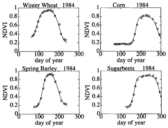
Figure 1.
Phenological tracks of several crops based on a vegetation index. Such tracks allow for the identification of characteristic times in crop development: emergence, full canopy, senescence, etc. The circles represent field observations; the solid line is a model fit [15]. Reprinted with permission from Ref. [15]. 2023, Elsevier.
Data of quality appropriate to support a detailed model typically require careful control of the study area, and if the data are collected with a satellite or aircraft platform, sufficient cloud-free conditions are necessary during each overpass. This is often not a realistic expectation and is a major drawback to using remote sensing for tracking the phenological stage of a crop [5]. Even when coarse-scale remote data are reliably available at weekly intervals, as with 5-day composite Advanced Very-High-Resolution Radiometer (AVHRR) data, the growth and senescence phases of individual crops cannot be distinguished using satellite data alone. AVHRR data have the further drawback of low spatial resolution, making it impossible to sample single crops [15].
When coupled with advanced machine learning and data processing, phenological tracking such as that in Figure 1 provides a reliable way of monitoring crop phenology [17]. However, scaling the process to commercial farms is cost- and skill-prohibitive, and it remains a tool specialized for crop-breeding programs. Other systems use low-cost cameras installed in the field called PhenoCams, which monitor the growth stages of the crop in real time [18,19]. While being more affordable and potentially more distributed than the high-throughput phenotyping platforms used in breeding programs, PhenoCams provide a localized estimation of crop phenology but still require development for adaptability to different environments, crop variety, crop status (e.g., healthy vs. stressed), etc. Using Unmanned Aerial Vehicles (UAVs) is yet another way to monitor crop phenology and is an approach that can achieve high levels of accuracy [20,21]. This platform also faces the same limitations in scalability when confronting ground and proximal sensing platforms, due to cost and skill requirements.
1.3. Challenges for the Remote Monitoring of Crop Phenology
Spectral imagery collected with satellites (or drones) remains a promising choice for the cost and scalability of crop phenology monitoring. However, certain challenges remain. Zeng et al. [16] provide a review of the phenological metrics derived from satellite data, concluding that the primary limitation is temporal resolution, which is seriously limited by the presence of cloud cover. Even if the temporal resolution issue can be overcome, the spatial resolution—necessary for the observation of single crops—remains an issue.
An effective approach that maintains both spatial and temporal resolution is to combine data from multiple satellites with comparable spatial resolution [22]. This approach increases the number of overpasses and reduces the problem of cloud cover while maintaining a reasonable spatial resolution, although there remain issues with radiometric calibration to account for differences in the spectral band placement and with the geometric registration of the ground sample points. As with the ground monitoring cited above, there have also been significant advances in applying machine learning to modeling remote sensing metrics to detect vegetation trends and fill gaps in remote sensing data [23,24].
A more fundamental problem, the problem addressed here, is the association of the phenological model with the day of year when considering growth patterns over multiple years or larger areas. This is illustrated in Figure 2 with NDVI data collected by the Hyperion imaging system on the EO-1 satellite from multiple corn fields over an 80-mile swath near Champaign, Illinois [25]. Each vertical set of points represents data from corn fields collected on a single day of the same year, with each point representing a single field. The spread of the data is indicative of differences in management (date of planting, irrigation, fertilization, etc.). While Hyperion data are capable of resolving individual fields and the general growth and decline of the corn crop is apparent, it would be impossible to extract any subtle details from this data presentation without other ground-based biophysical properties (e.g., planting date). Even at higher resolution and higher frequency, the land surface phenological stages are roughly estimated (e.g., “Start of greenness rising Season” or “End of greenness falling Season”), and their accuracy remains limited. Diao and Li (2022) Showed r2 values of 0.64 for detecting emergence and 0.58 for detecting crop maturity using PlanetScope data [26]. The limited accuracy obtained when using single-index approaches without ground-based biophysical properties seems to be linked to all indices following an increasing and decreasing trajectory that fully overlaps (i.e., a scalar quantity).
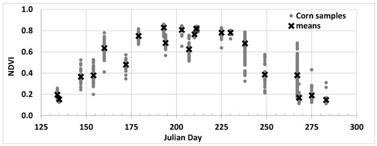
Figure 2.
NDVI observations from the Hyperion scanner on the EO-1 satellite collected over a 7-year period [25]. Each vertical collection of points is from a single year. The variability (e.g., average NDVI decreasing and increasing again) is mainly due to differences in day of planting across the different years.
1.4. Using Paired Normalized Spectral Indices in ND-Space Can Significantly Improve Crop Phenology Monitoring Performed Using Remote Sensing
A notable difficulty in the use of vegetative indices in general has been the focus on reducing the description of the crop state to a scalar quantity. Even a two-dimensional map can facilitate modeling and classification [27]. A two-dimensional index would allow for the characterization of distinct crop characteristics and has the potential to be much more descriptive overall [6]. The hypothesis is that by using both a canopy chlorophyll content index (e.g., NDVI) and a canopy water content index (e.g., NDWI) in a two-dimensional normalized difference space (ND-space), one can classify crop phenological stages significantly better than by using either of these indices alone. This has the additional advantage of avoiding the constraint imposed by tying the phenology to the day of year (DOY) or Julian day (JD).
The Normalized Difference Vegetation Index (NDVI), typically used for estimating crop properties, is primarily sensitive to the pigment concentration and cell structure of plants [28]. It is most typically used as a measure of vegetation density, but the relationship is non-linear and thus not consistent throughout the crop growing season [29]. The NDVI is also indirectly sensitive to water content [30] and has been used as an indirect indicator of water stress (e.g., [31]). Used alone, the NDVI is thus not sufficient for reliably estimating crop phenology, because the same NDVI value can indicate different growth stages (e.g., an NDVI value of 0.7 could mean late growth or early senescence, or late growth under water stress).
Another way of monitoring a crop is to use the shortwave infrared (SWIR), which can be linked to the water content in the pixel [32]. The basis of this approach is that greater biomass translates into more water in the pixel, which can be detected using satellite-based SWIR. The SWIR part of the spectrum has also been used to estimate non-photosynthetic vegetation cover relative to soil cover, which may indicate that chlorophyll-based vegetation indices (e.g., NDVI) and SWIR-based vegetation indices may follow different time series [33]. As with the NDVI, SWIR measurements would not be able to distinguish between a young plant and a senescing plant if both exhibited comparable water content on a pixel basis. Accordingly, a study using hyperspectral data and machine learning found that important wavebands for predicting crop phenological stages are 700–800 nm and 800–1300 nm, and the results seemed to indicate that both wavebands play a role in adequately measuring crop phenological stages [34].
There is significant precedent for multi-dimensional analyses with remote sensing data [35]. The triangle method, introduced by Price [36] and developed by several others [37], uses a scatterplot of surface radiant temperature vs. a vegetation index to estimate soil surface wetness and evapotranspiration fraction from satellite imagery. Spectral mixture analysis is often used with hyperspectral data to characterize pixels representing multiple pure materials as well as discriminating mixtures of those materials [38,39]. Particularly relevant to the work presented here is the use of spectral mixture analysis to discriminate among bare soil, vegetation, and non-photosynthetic vegetation [40] by contrasting the NDVI with the cellular absorption index (CAI), a shortwave infrared index designed to track the depth of the cellulose absorption band [41]. Guerschman et al. [40] used this approach to estimate the fractional cover of bare soil, and photosynthetic and non-photosynthetic vegetation in the Australian tropical savanna region and expanded the analysis to three dimensions using a ratio of the SWIR bands from MODIS. A similar approach was taken more recently to assess crop leaf chlorophyll content and fractional cover, using angular measures in the 2D scatterplot space [27].
While this is only a sampling of the work that has been carried out using multi-dimensional analyses, all of the work has focused on analysis of single images; to our knowledge, none have addressed time-varying characteristics appropriate to phenological modeling. In this paper, we examine the possibility of using the relatively simple ND-space defined with the NDVI and a second SWIR-NIR index to track the time-varying reflectance that changes associated with crop phenology. The specific objectives of this study are (1) to observe if using the ND-space can provide additional information for monitoring crop phenology and (2) to interpret observations and pose research questions that could allow for further exploration of this new approach. Although only four wavebands are ultimately required, we explore the possible wavelength combinations using hyperspectral data, since this allows for consideration of many more possible band combinations. The goal of this publication is to demonstrate a new way of looking at remote sensing data time series for crop phenology monitoring.
2. Materials and Methods
2.1. Crop Phenological Data
2.1.1. The GHISA Spectral Data Set
The work described here relies on the Global Hyperspectral Imaging Spectral library of Agricultural crops (GHISA) [25,42] data collected by the Hyperion hyperspectral imaging sensor aboard the EO-1 spacecraft. At the time of writing this article, GHISA is the only known database that is publicly available and analysis-ready for application to a crop phenology study integrating both spectral and ground observations. The spectral range of the imaging system spans the visible, near-infrared (NIR), and shortwave infrared (SWIR), with a spatial resolution of 30 m. GHISA products provide radiometrically calibrated and atmospherically corrected reflectance spectra covering the spectral range 437–2345 nm and are spectrally sorted into 5 categories representing the 5 leading crop types in the world: corn, soybean, winter wheat, rice, and cotton. Data were collected throughout the growing season on cloud-free days and are broadly categorized by growth stage. The year, Julian date, and location of each sample spectrum is provided. The crop type for each field was retrieved from the USDA Crop Data Layer (CDL) database [43].
While there are known difficulties in the radiometric and wavelength calibration of Hyperion data, reflectance time series have been shown to be stable and suitable for monitoring vegetation functional parameters, including NDVI, EVI, feature depth, and 1st derivatives [44]. Some of the Hyperion data acquired with the EO-1 satellite suffered a drift from sun synchronous precession orbit when the satellite ran out of onboard maneuvering fuel in 2011, which can result in reduced signal quality associated with weaker irradiance and a longer atmospheric path for radiance to traverse [45,46]. However, the data show that “no marked trend in decreasing quality in Hyperion is apparent through 2016, and these data remain a high quality resource through the end of the mission” [45]. The Hyperion data used here include images collected between 2009 and 2015 from a single EO-1 path over Champaign County in Illinois, USA, in an area where corn and soybeans are grown. The locations of the individual fields are shown in Figure 3. Spectral data from 22 separate overpasses were associated with both the corn and soybean crops (Figure 4). As there is only a very rough indication of the crop status for individual fields for any given overpass in the CDL database, it is necessary to rely on the spectral reflectance to sort the data into a sequence of growth stages.
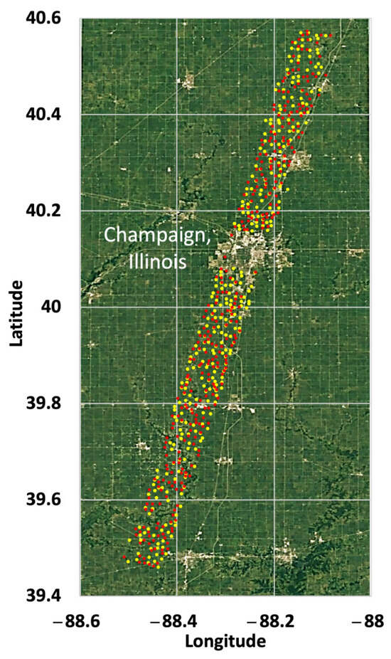
Figure 3.
Map showing the locations of corn (yellow) and soybean (red) fields in the County of Champaign, IL, USA, that were used for this analysis.
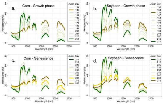
Figure 4.
Averaged spectra collected during each EO-1 overpass: (a) progression from bare soil (brown) to maximum corn vegetation (green); (b) progression from bare soil (brown) to maximum soybean vegetation (green); (c) progression from maximum corn vegetation (green) to non-photosynthetic vegetation (NPV; yellow to brown); (d) progression from maximum soybean vegetation (green) to non-photosynthetic vegetation (NPV; yellow to brown).
The 14 mean corn crop spectra representing the progression from bare soil (thick brown line) to maximum vegetation (thick green line) are shown in Figure 4a for corn and in Figure 4b for soybean. Individual spectra are numbered in chronological order by Julian day (JD). Since the data span seven years and growing conditions vary from year to year, JD is not a precise measure of crop status from year to year. Yearly variations explain the early-season spectra for both corn and soybean, in that the mean spectrum for JD 135 from 2013 (thick brown line) appears to be more characteristic of bare soil than the mean spectrum for JD 134 from 2012 and, in the case of the soybean crop, JD 130 from 2014.
The spectral change during the latter half of the growing season, from mature crop to non-photosynthetic vegetation (NPV; thick gold line) is shown for corn in Figure 4c and for soybean in Figure 4d, again represented by the mean spectra for each JD. In this case, there is an 18 JD day gap (JD 249 to JD 267) from early senescence to late senescence for corn—likely due to problems with cloud cover—that appears as a gap in the spectra in the NIR range (Figure 4c). The same time gap exists in the soybean data (Figure 4d) but is not obvious in the spectra.
The mean spectra for bare soil in both the corn and soybean fields are very similar (Figure 4a,b). The full canopy spectra for corn and soybean are nearly identical in the visible, but the soybean spectrum is consistently brighter throughout the infrared. The spectra of late-season senesced vegetation, which we designate as NPV (thick orange curve in Figure 4c,d), look very similar to the bare soil spectra (thick brown curve). For corn, the bare soil and NPV spectra (Figure 4c) are nearly identical in the visible and near infrared (VNIR) but differentiate in the SWIR. For soybean (Figure 4d), the NPV reflectance is brighter than the bare soil reflectance in the VNIR while the two are very similar in the SWIR.
2.1.2. Pigment, Cell Structure, and Water Content
Pigment concentration is characterized by absorption (decrease in reflectance) in the visible spectrum (400–700 nm). In the NIR and the shorter wavelength range of the SWIR (700–1300 nm), light is scattered very effectively, but there is relatively little absorption either by plant pigments or by water [47]. In the far-SWIR (1300–2500 nm), scattering is still effective, and there is no absorption by pigments; however, absorption by water increases dramatically with wavelength [48]. A straightforward approach to capturing these differences is to focus on the changes in spectral slope: the increase in slope from the red to the infrared is tied to the increase in absorption by plant pigments in the visible and the increase in scattering in the NIR and is well represented by the NDVI. A similar normalized difference metric contrasting the NIR/near-SWIR with the far-SWIR has the potential to capture the changes in water content.
2.2. Normalized Difference Metrics
A previous paper [6] made the case for using pairs of normalized difference (ND) metrics for capturing and analyzing spectral change in multi- and hyperspectral images. ND metrics are essentially scaled slopes and are insensitive to changes in brightness that confound the characterization of color changes. This property underlies the effectiveness of the NDVI and many other related scalar indices [17]. The NDVI, a parameter first used in the early years of satellite image data [49], is valued for its sensitivity to biomass or vegetation density, and its insensitivity to soil moisture. It is, however, insensitive to leaf water content and is also unable to distinguish between soil and NPV, limiting its potential for tracking a full crop life cycle. While the NDVI is proven to saturate for grass crops, it was used for the purpose of this demonstration study because it is a well-known index for characterizing chlorophyll concentration, and saturation does not prevent the demonstration in this case [50]. Red and NIR wavelengths were chosen within the Hyperion data and define the NDVI in Equation (1).
NDVI = (NIRa − Red)/NIRa + Red)
Red = 681 nm, NIRa = 854 nm
Red = 681 nm, NIRa = 854 nm
Combining the NDVI with an ND metric that is sensitive to leaf water content would have the potential to discriminate between growing and senescing crops. Multiple indices have been proposed for representing the moisture content of vegetation. It has long been recognized that the sensitivity to the presence of water is better at NIR and SWIR wavelengths [51,52] due to strong absorption by water at these wavelengths, but algorithms were initially restricted by the spectral bands available on the multispectral imaging satellites of the time. With the increasing availability of hyperspectral imagery, several newer vegetation water indices have been proposed with more precise band selection both in the NIR [53] and in the SWIR [54]. Indices relying on the NIR are advantageous because of the insensitivity of normalized difference indices to soil moisture in this spectral range [55], as well as the broader availability (and lower expense) of hyperspectral sensors covering this range [56]. On the other hand, the water absorption coefficient increases by orders of magnitude between 900 nm and 2500 nm [48], suggesting that SWIR bands are likely to provide more sensitivity, although a normalized difference index in this spectral range may be affected by both leaf and soil water contents [57]. We define NDSW, a normalized difference metric that contrasts the reflectance at the long-wavelength end of the visible and near-infrared with the reflectance at the long-wavelength end of the SWIR:
NDSW = (SWIR − NIRb)/SWIR + NIRb)
NIRb = 912 nm, SWIR = 2103 nm
NIRb = 912 nm, SWIR = 2103 nm
NDSW is presumed here to be primarily sensitive to vegetation water content, whether the vegetation is still growing or is senescing.
In selecting band pairs for the normalized difference, it is the slope of the line connecting the two chosen bands that is the most important. Figure 5 illustrates the slopes represented by the NDVI and NDSW. The NDVI provides a strong contrast between the vegetation, and both bare soil and NPV, and a smaller slope difference between soil and NPV. The slopes represented by NDSW also differentiate among vegetation, soil, and NPV; however, there is also a small but significant difference in the slopes of bare soil (positive) and NPV (negative). Note that the slopes of each of the three targets are similar for both corn and soybean spectra in Figure 5b, although the reflectance magnitude is different.
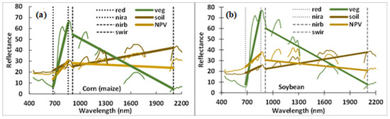
Figure 5.
Spectral slopes of soil, vegetation, and NPV (non-photosynthetic vegetation) represented by the NDVI and a normalized difference (NDSW) linking the near-infrared at 912 nm (nirb) and the shortwave infrared at 2103 nm (swir) for corn (a) and soybean (b).
3. Results
An ND-space plot of NDVI and NDSW for the full GHISA corn and soybean data sets for the Illinois Hyperion path reveals a progression throughout the growing season from bare soil to mature crops, then from senescence to NPV, and finally returning to bare soil (Figure 6). The data representing the progression from bare soil (JD 135) to full vegetation (JD 211) are bounded with green lines; the data representing the progression from full vegetation to NPV (JD 268) are bounded with brown lines. The lines are exponential functions similar to those derived in [6], connecting representative samples (e.g., bare soil and full canopy). The NDVI represents the contrast in absorption by photosynthetic pigments in the visible with the increase in scattering in the near-infrared. NDSW is presumed to represent the change in water content.
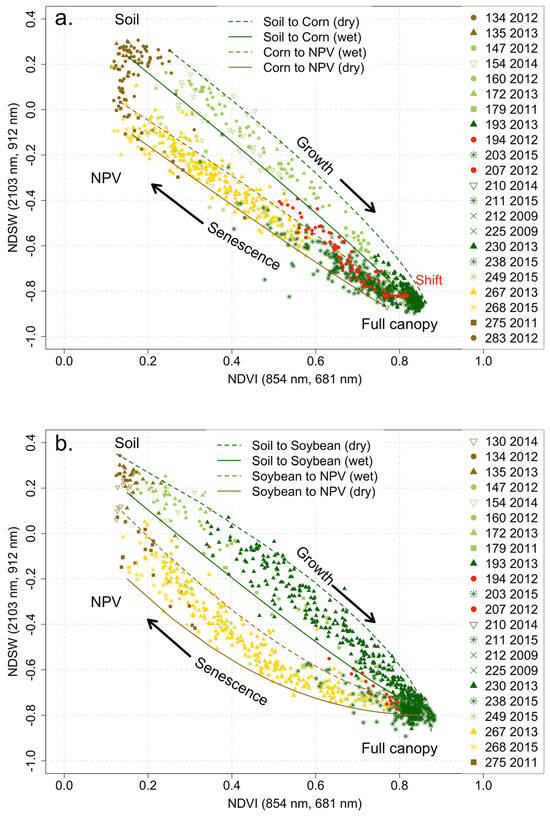
Figure 6.
ND-space (NDVI vs. NDSW) representations of the complete GHISA data set for corn (a) and soybean (b) crops in the Illinois study area. Similarly shaped data points represent data from the same year. Colors are intended to represent growth stages. The mean spectra of these data sets are the spectra displayed in Figure 4. Red symbols indicate data recorded during the 2012 exceptional drought event. Solid and dashed lines are exponential functions fit to representative bounding values (e.g., bare dry soil, dense vegetation) to provide a visual guide.
The plot for the corn data (Figure 6a) follows a nearly linear track (cluster bounded by green lines) throughout the growing season from bare soil (brown) to mature (green) crop. A similar linear pattern is seen for the return to NPV (cluster bounded by brown lines). When the crop is at full canopy, there appears to be an initial shift in the NDVI while NDSW remains stable—possibly the result of tasseling. The corn tassels at the top of the plant would present a non-photosynthetic surface and partially block the light reflected from the leaves below.
The overall pattern is somewhat similar for soybean (Figure 6b), but with interesting differences. During the growth phase, the points again follow a nearly linear track (solid green line), but with greater overall variability (curved green line). During senescence, however, the points follow a noticeably curved path. There is initially a more rapid decrease in NDSW than in NDVI. The rates of change draw closer together as senescence progresses, with the path becoming roughly linear toward the end. For both corn and soybean, the senescence track ends with an NDVI value equivalent to that of bare soil (NDVI ≈ 0.08) but with NDSW being negative and lower than that for soil, suggesting that NPV initially maintains some moisture but dries over time.
An interesting complication occurred in 2012 when there was a severe drought in Illinois (Figure 7). The drought was initially moderate but became increasingly severe in mid-June 2012 and was declared exceptional in late July 2012 [58]. This pattern is reflected in the ND-space plots in Figure 6. The early-2012 data (JD 134, 147, and 160) follow the same pattern as those from other years, but data collected during the serious drought in mid- to late July (JD 194 and 207) are shifted out of line with data from other years. The shift corresponds to lower NDSW, consistent with lower water content. It could also be indicative of a pigment reduction. There are no data from 2012 after JD 207 except for the one set of corn data at the end of the season, in October (JD 283).
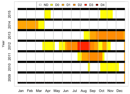
Figure 7.
Drought intensity index on a weekly basis from 2009 to 2015 for the County of Champaign in Illinois, USA. The legend indicates the following: ND: no drought; D0: abnormally dry; D1: moderate drought; D2: severe drought; D3: extreme drought; and D4: exceptional drought. Data source: National Integrated Drought Information System, NOAA, accessible at www.drought.gov (accessed on 14 November 2023).
The non-drought data presented in Figure 6 show distinct, repeatable patterns, although they represent multiple fields spanning a large area (Figure 3), multiple years, and presumably a range of soil treatments and management practices on individual farms. The bare soil points cluster along a vertical line in the ND-space (NDVI ≈ 0.08), most likely depending on the moisture level, and merge with the NPV points. A mature canopy of the same crop would be likely to have the same location in the ND-space. In the ND-space plot for corn and soybean crops (Figure 6), the locus of mature crops differs slightly but consistently, with the NDVI for corn (NDVI ≈ 0.82) being noticeably lower than that for soybean (NDVI ≈ 0.87) possibly because of the tassels that remain at the top of the plants. It is also reasonable to expect that NPV would occupy the same location, regardless of vegetation types.
Overall, Figure 6 clearly shows that within the ND-space defined by NDVI and NDSW, each crop exhibits a combination of spectral reflectance properties that are distinct throughout the crop growing season from planting to senescence. Indeed, as compared with the scalar NDVI or scalar NDSW, in the ND-space shown here, there is a notable distinction between the growing and senescence phases, thus providing information on the stage of the crop (i.e., corn or soybean) at any time of the crop growing season.
4. Discussion
The dominant message of the plots in Figure 6 is that the phenological state is distinguishable from emergence through full canopy to senescence. The two-dimensional plot is essential; neither the NDVI nor NDSW can differentiate between growth or senescence alone, but the two indices together clearly distinguish the full sequence of growth stages. There may be more information in this type of plot, however. As suggested in the presentation, we would like to postulate a more detailed interpretation under the premises that (a) the NDVI is sensitive to pigment concentration and cell structure but is essentially insensitive to leaf water content and that (b) NDSW is distinctly sensitive to the presence of water (whether in soil or vegetation), while its sensitivity to pigment concentration/cell structure is highly correlated with that of the NDVI. If these premises are true, then a change along the x-axis of the ND-space plot (Figure 4) indicates a change in pigment concentration, and a change along the y-axis indicates a change in water content.
The following observations can then be made:
- During the growth phase, the vertical scatter of data for any NDVI value may indicate a range of moisture content; the horizontal scatter of data for any NDSW value may indicate a range of pigment content. This observation is supported by the shift to lower NDSW values for the data collected during the 2012 drought.
- At full canopy, corn appears to lose pigment, while the water content remains stable. There is no such shift for the soybean crop. This is likely attributable to the formation of tassels (between JD 211 and JD 225); the chlorophyll content of tassels is lower than that of leaves, but they have similar water content. Tassels appearing at the top of the plant may obstruct part of the leaf canopy from the nadir view of the remote sensing image and may produce a shift in NDVI that is apparent in the ND-space.
- During senescence, the corn crop appears to lose pigment and water at about the same rate over the entire senescence period. The resulting senescence track closely parallels the growth track.
- During senescence, the soybean crop initially appears to lose pigment, while the water content is relatively stable, but about midway through senescence, the rates become more equal.
- During senescence, the vertical scatter of data for any NDVI value may indicate a range of moisture content; the horizontal scatter of data for a given NDSW value may indicate a difference in pigment concentration.
- When pigments are entirely gone (NDVI ≈ 0.08, no pigment), there is still water remaining in NPV or soil. As the NPV or soil dries, NDSW approaches the value of bare soil.
Using the ND-space to observe crop growth opens new perspectives for the use of remote sensing data to monitor crop phenology and may thus deserve the attention of the scientific community to develop its potential. There are important aspects of this approach that require further research to define the expansion capacity and reliability for monitoring crop phenology in detail.
In this study, the NDVI and NDSW were used to define the ND-space and seem to have good potential for discriminating growth stages throughout the crop growing season. This was deemed sufficient for the scope of this study, aiming to present this new way of using remote sensing data. Other indices may provide more detail; however, normalized differences have the advantage of simplicity, insensitivity to the magnitude of reflectance, and scaling in the range [−1, +1]. Optimizing and understanding the choice of ND indices for discriminating crop phenological stages is important to further develop this approach.
The data set used here provided six (corn) or seven (soybean) broad phenological stages from emergence to harvest. While this can be useful in general, certain uses may require more detailed monitoring of phenological growth stages [59]. Further research with ground-truth data detailing crop phenological stages (e.g., number of leaves for corn) would thus be needed to develop an algorithm capable of utilizing the ND-space for this purpose across different crops.
The two indices used seem to characterize distinct attributes of crop canopy; notably, the NDVI characterizes its chlorophyll content, and NDSW, its water content. While the assumption is that both distinctively characterize those components, further research is needed to establish the specificity and interdependency of those relationships. This requires actual canopy chlorophyll and water content ground measurements.
5. Conclusions
This paper presents an approach for tracking crop phenology throughout the growing season, clearly distinguishing between the growth phase and the senescence phase, with an indication of the possibility of also distinguishing NPV. The analysis relies on a unique collection of hyperspectral satellite data associated with individual corn and soybean fields spanning the full crop cycle over seven years. Based on a pair of normalized difference metrics, the results are independent of the magnitude of reflectance. Band pairs are selected to highlight spectral differences that are associated with distinct properties: NDVI is responsive to plant pigment concentration, and NDSW is sensitive to water content.
The resulting plots are very suggestive, indicating that it is not only possible to distinguish between growth and senescence but that it is probable that the stage of development might be retrieved. There are also differences in the shapes of the patterns for corn and soybean that appear to be characteristic of the individual crops. The fact that the data for both crops are consistent over a 7-year span covering multiple fields and two distinct crops suggests that the results are significant and should be repeatable.
Nonetheless, this is essentially an exercise in data mining using a remarkable collection of hyperspectral satellite data. Conclusions are based only on an identified crop, a Julian date, and locations for which reflectance spectra are available. There is no ground truth to verify the crop condition (e.g., plant health, water content, weed cover, etc.). Nor is there information on the actual growth stage of the crops (e.g., six-leaf corn).
The results are very suggestive, with the ND-space representation of the NDVI–NDSW pair showing great potential to monitor crop phenology, but require controlled studies to verify the relationships, especially to verify the water content relationship. The approach should be further tested to examine the actual relationship of the ND-space patterns and the precise growth stages and to determine the actual effect of differences in chlorophyll content and water content. Finally, it remains to be examined how well this approach would apply to other crops and to consider effects that are specific to a particular crop, e.g., the appearance of tassels on corn or flowering on soybean.
Author Contributions
Conceptualization, L.L. and W.P.; methodology, L.L. and W.P.; software, L.L. and W.P.; validation, L.L. and W.P.; formal analysis, L.L. and W.P.; investigation, L.L. and W.P.; resources, L.L. and W.P.; data curation, public; writing—original draft preparation, L.L. and W.P.; writing—review and editing, L.L. and W.P.; visualization, L.L. and W.P.; supervision, L.L. and W.P.; project administration, NA; funding acquisition, NA. All authors have read and agreed to the published version of the manuscript.
Funding
This research received no external funding.
Data Availability Statement
The data are publicly available at https://www.usgs.gov/media/files/ghisa-usa-eo-1-hyperion-dataset (accessed on 14 November 2023).
Acknowledgments
This study was made possible by free access to the GHISA data set provided by US Geological Survey.
Conflicts of Interest
The authors declare no conflict of interest.
References
- Soudani, K.; Francois, C. A Green Illusion. Nature 2014, 506, 165–166. [Google Scholar] [CrossRef] [PubMed]
- Diao, C. Remote Sensing Phenological Monitoring Framework to Characterize Corn and Soybean Physiological Growing Stages. Remote Sens. Environ. 2020, 248, 111960. [Google Scholar] [CrossRef]
- Fageria, N.K.; Baligar, V.C.; Clark, R.B.; Ralph, B. Physiology of Crop Production; Food Products Press: Devon, UK, 2006; ISBN 9781560222897. [Google Scholar]
- Soffe, R.J.; Lobley, M. The Agricultural Notebook, 21st ed.; Wiley-Blackwell: Hoboken, NJ, USA, 2021; ISBN 978-1-119-56036-4. [Google Scholar]
- Gao, F.; Zhang, X. Mapping Crop Phenology in Near Real-Time Using Satellite Remote Sensing: Challenges and Opportunities. J. Remote Sens. 2021, 2021, 8379391. [Google Scholar] [CrossRef]
- Philpot, W.; Jacquemoud, S.; Tian, J. ND-Space: Normalized Difference Spectral Mapping. Remote Sens. Environ. 2021, 264, 112622. [Google Scholar] [CrossRef]
- Menzel, A. Phenology: Its Importance to the Global Change Community: An Editorial Comment. Clim. Chang. 2002, 54, 379–385. [Google Scholar] [CrossRef]
- Seo, B.; Lee, J.; Lee, K.D.; Hong, S.; Kang, S. Improving Remotely-Sensed Crop Monitoring by NDVI-Based Crop Phenology Estimators for Corn and Soybeans in Iowa and Illinois, USA. Field Crops Res. 2019, 238, 113–128. [Google Scholar] [CrossRef]
- Hegarty-Craver, M.; Polly, J.; O’Neil, M.; Ujeneza, N.; Rineer, J.; Beach, R.H.; Lapidus, D.; Temple, D.S. Remote Crop Mapping at Scale: Using Satellite Imagery and UAV-Acquired Data as Ground Truth. Remote Sens. 2020, 12, 1984. [Google Scholar] [CrossRef]
- Longchamps, L.; Panneton, B.; Simard, M.-J.; Leroux, G.D. An Imagery-Based Weed Cover Threshold Established Using Expert Knowledge. Weed Sci. 2014, 62, 177–185. [Google Scholar] [CrossRef]
- Boschetti, M.; Stroppiana, D.; Brivio, P.A.; Bocchi, S. Multi-Year Monitoring of Rice Crop Phenology through Time Series Analysis of MODIS Images. Int. J. Remote Sens. 2009, 30, 4643–4662. [Google Scholar] [CrossRef]
- Templ, B.; Koch, E.; Bolmgren, K.; Ungersböck, M.; Paul, A.; Scheifinger, H.; Rutishauser, T.; Busto, M.; Chmielewski, F.-M.; Hájková, L.; et al. Pan European Phenological Database (PEP725): A Single Point of Access for European Data. Int. J. Biometeorol. 2018, 62, 1109–1113. [Google Scholar] [CrossRef]
- Sadeghi-Tehran, P.; Sabermanesh, K.; Virlet, N.; Hawkesford, M.J. Automated Method to Determine Two Critical Growth Stages of Wheat: Heading and Flowering. Front. Plant Sci. 2017, 8, 252. [Google Scholar] [CrossRef] [PubMed]
- Jin, X.; Zarco-Tejada, P.J.; Schmidhalter, U.; Reynolds, M.P.; Hawkesford, M.J.; Varshney, R.K.; Yang, T.; Nie, C.; Li, Z.; Ming, B.; et al. High-Throughput Estimation of Crop Traits: A Review of Ground and Aerial Phenotyping Platforms. IEEE Geosci. Remote Sens. Mag. 2021, 9, 200–231. [Google Scholar] [CrossRef]
- Fischer, A. A Model for the Seasonal Variations of Vegetation Indices in Coarse Resolution Data and Its Inversion to Extract Crop Parameters. Remote Sens. Environ. 1994, 48, 220–230. [Google Scholar] [CrossRef]
- Zeng, L.; Wardlow, B.D.; Xiang, D.; Hu, S.; Li, D. A Review of Vegetation Phenological Metrics Extraction Using Time-Series, Multispectral Satellite Data. Remote Sens. Environ. 2020, 237, 111511. [Google Scholar] [CrossRef]
- Xue, J.; Su, B. Significant Remote Sensing Vegetation Indices: A Review of Developments and Applications. J. Sens. 2017, 2017, 1353691. [Google Scholar] [CrossRef]
- Taylor, S.D.; Browning, D.M. Classification of Daily Crop Phenology in PhenoCams Using Deep Learning and Hidden Markov Models. Remote Sens. 2022, 14, 286. [Google Scholar] [CrossRef]
- Liu, Y.; Bachofen, C.; Wittwer, R.; Duarte, G.S.; Sun, Q.; Klaus, V.H.; Buchmann, N. Using PhenoCams to Track Crop Phenology and Explain the Effects of Different Cropping Systems on Yield. Agric. Syst. 2022, 195, 103306. [Google Scholar] [CrossRef]
- Pugh, N.A.; Horne, D.W.; Murray, S.C.; Carvalho, G.; Malambo, L.; Jung, J.; Chang, A.; Maeda, M.; Popescu, S.; Chu, T.; et al. Temporal Estimates of Crop Growth in Sorghum and Maize Breeding Enabled by Unmanned Aerial Systems. Plant Phenome J. 2018, 1, 1–10. [Google Scholar] [CrossRef]
- Yang, Q.; Shi, L.; Han, J.; Yu, J.; Huang, K. A near Real-Time Deep Learning Approach for Detecting Rice Phenology Based on UAV Images. Agric. For. Meteorol. 2020, 287, 107938. [Google Scholar] [CrossRef]
- Moon, M.; Richardson, A.D.; Friedl, M.A. Multiscale Assessment of Land Surface Phenology from Harmonized Landsat 8 and Sentinel-2, PlanetScope, and PhenoCam Imagery. Remote Sens. Environ. 2021, 266, 112716. [Google Scholar] [CrossRef]
- Belda, S.; Pipia, L.; Morcillo-Pallarés, P.; Rivera-Caicedo, J.P.; Amin, E.; Grave, C.D.; Verrelst, J. DATimeS: A Machine Learning Time Series GUI Toolbox for Gap-Filling and Vegetation Phenology Trends Detection. Environ. Model. Softw. 2020, 127, 104666. [Google Scholar] [CrossRef]
- Eklundh, L.; Jönsson, P. TIMESAT 3.3 with Seasonal Trend Decomposition and Parallel Processing 2017. Available online: https://web.nateko.lu.se/timesat/docs/TIMESAT33_SoftwareManual.pdf (accessed on 19 September 2023).
- Thenkabail, P.; Aneece, I. Global Hyperspectral Imaging Spectral-Library of Agricultural Crops for Conterminous United States V001. NASA EOSDIS Land Processes DAAC 2019. Available online: https://cmr.earthdata.nasa.gov/search/concepts/C1629302681-LPDAAC_ECS.html (accessed on 19 September 2023).
- Diao, C.; Li, G. Near-Surface and High-Resolution Satellite Time Series for Detecting Crop Phenology. Remote Sens. 2022, 14, 1957. [Google Scholar] [CrossRef]
- Yue, J.; Tian, J.; Philpot, W.; Tian, Q.; Feng, H.; Fu, Y. VNAI-NDVI-Space and Polar Coordinate Method for Assessing Crop Leaf Chlorophyll Content and Fractional Cover. Comput. Electron. Agric. 2023, 207, 107758. [Google Scholar] [CrossRef]
- Adams, M.L.; Philpot, W.D.; Norvell, W.A. Yellowness Index: An Application of Spectral Second Derivatives to Estimate Chlorosis of Leaves in Stressed Vegetation. Int. J. Remote Sens. 1999, 20, 3663–3675. [Google Scholar] [CrossRef]
- Glenn, E.P.; Huete, A.R.; Nagler, P.L.; Nelson, S.G. Relationship Between Remotely-Sensed Vegetation Indices, Canopy Attributes and Plant Physiological Processes: What Vegetation Indices Can and Cannot Tell Us about the Landscape. Sensors 2008, 8, 2136–2160. [Google Scholar] [CrossRef] [PubMed]
- Zhao, T.; Stark, B.; Chen, Y.; Ray, A.L.; Doll, D. A Detailed Field Study of Direct Correlations between Ground Truth Crop Water Stress and Normalized Difference Vegetation Index (NDVI) from Small Unmanned Aerial System (sUAS). In Proceedings of the 2015 International Conference on Unmanned Aircraft Systems (ICUAS), Denver, CO, USA, 9–12 June 2015; IEEE: New York, NY, USA, 2015; pp. 520–525. [Google Scholar]
- Gu, Y.; Brown, J.F.; Verdin, J.P.; Wardlow, B. A Five-Year Analysis of MODIS NDVI and NDWI for Grassland Drought Assessment over the Central Great Plains of the United States. Geophys. Res. Lett. 2007, 34, L06407. [Google Scholar] [CrossRef]
- Jenal, A.; Hüging, H.; Ahrends, H.E.; Bolten, A.; Bongartz, J.; Bareth, G. Investigating the Potential of a Newly Developed UAV-Mounted VNIR/SWIR Imaging System for Monitoring Crop Traits—A Case Study for Winter Wheat. Remote Sens. 2021, 13, 1697. [Google Scholar] [CrossRef]
- Hively, W.D.; Lamb, B.T.; Daughtry, C.S.T.; Serbin, G.; Dennison, P.; Kokaly, R.F.; Wu, Z.; Masek, J.G. Evaluation of SWIR Crop Residue Bands for the Landsat Next Mission. Remote Sens. 2021, 13, 3718. [Google Scholar] [CrossRef]
- Doktor, D.; Lausch, A.; Spengler, D.; Thurner, M. Extraction of Plant Physiological Status from Hyperspectral Signatures Using Machine Learning Methods. Remote Sens. 2014, 6, 12247–12274. [Google Scholar] [CrossRef]
- Landgrebe, D.A. Machine Processing for Remotely Acquired Data. LARS Tech. Rep. 1973, 1–29. Available online: https://docs.lib.purdue.edu/larstech/109/ (accessed on 19 September 2023).
- Price, J.C. On the Information Content of Soil Reflectance Spectra. Remote Sens. Environ. 1990, 33, 113–121. [Google Scholar] [CrossRef]
- Carlson, T.N. An Overview of the “Triangle Method” for Estimating Surface Evapotranspiration and Soil Moisture from Satellite Imagery. Sensors 2007, 7, 1612–1629. [Google Scholar] [CrossRef]
- Adams, J.B.; Smith, M.O.; Johnson, P.E. Spectral Mixture Modeling: A New Analysis of Rock and Soil Types at the Viking Lander 1 Site. J. Geophys. Res. Solid Earth 1986, 91, 8098–8112. [Google Scholar] [CrossRef]
- Bell, J.F.; Farrand, W.H.; Johnson, J.R.; Morris, R.V. Low Abundance Materials at the Mars Pathfinder Landing Site: An Investigation Using Spectral Mixture Analysis and Related Techniques. Icarus 2002, 158, 56–71. [Google Scholar] [CrossRef][Green Version]
- Guerschman, J.P.; Hill, M.J.; Renzullo, L.J.; Barrett, D.J.; Marks, A.S.; Botha, E.J. Estimating Fractional Cover of Photosynthetic Vegetation, Non-Photosynthetic Vegetation and Bare Soil in the Australian Tropical Savanna Region Upscaling the EO-1 Hyperion and MODIS Sensors. Rem. Sens. Environ. 2009, 113, 928–945. [Google Scholar] [CrossRef]
- Nagler, P.L.; Daughtry, C.S.T.; Goward, S.N. Plant Litter and Soil Reflectance. Remote Sens. Environ. 2000, 71, 207–215. [Google Scholar] [CrossRef]
- Aneece, I.; Thenkabail, P. Accuracies Achieved in Classifying Five Leading World Crop Types and Their Growth Stages Using Optimal Earth Observing-1 Hyperion Hyperspectral Narrowbands on Google Earth Engine. Remote Sens. 2018, 10, 2027. [Google Scholar] [CrossRef]
- USDA. CroplandCROS, CropScape, and Cropland Data Layer. Available online: https://croplandcros.scinet.usda.gov/ (accessed on 19 September 2023).
- Felde, G.W.; Anderson, G.P.; Cooley, T.W.; Matthew, M.W.; adler-Golden, S.M.; Berk, A.; Lee, J. Analysis of Hyperion Data with the FLAASH Atmospheric Correction Algorithm. In Proceedings of the International Geoscience and Remote Sensing Symposium; Proceedings (IEEE Cat. No.03CH37477), Toulouse, France, 21–25 July 2003; IEEE Geoscience and Remote Sensing Society: Toulouse, France, 2003; Volume 1, pp. 90–92. [Google Scholar]
- Franks, S.; Neigh, C.S.R.; Campbell, P.K.; Sun, G.; Yao, T.; Zhang, Q.; Huemmrich, K.F.; Middleton, E.M.; Ungar, S.G.; Frye, S.W. EO-1 Data Quality and Sensor Stability with Changing Orbital Precession at the End of a 16 Year Mission. Remote. Sens. 2017, 9, 412. [Google Scholar] [CrossRef]
- Swinnen, E.; Verbeiren, S.; Deronde, B.; Henry, P. Assessment of the Impact of the Orbital Drift of SPOT-VGT1 by Comparison with SPOT-VGT2 Data. Int. J. Remote Sens. 2014, 35, 2421–2439. [Google Scholar] [CrossRef]
- Ustin, S.L.; Jacquemoud, S. How the Optical Properties of Leaves Modify the Absorption and Scattering of Energy and Enhance Leaf Functionality. In Remote Sensing of Plant Biodiversity; Springer International Publishing: Cham, Switzerland, 2020; pp. 349–384. [Google Scholar]
- Kou, L.; Labrie, D.; Chylek, P. Refractive Indices of Water and Ice in the 0.65–2.5 mm Spectral Range. Appl. Opt. 1993, 32, 3531–3540. [Google Scholar] [CrossRef]
- Rouse, J.W.; Hass, R.H.; Schell, J.A.; Deering, D.W. Monitoring Vegetation Systems in the Great Plains with ERTS. Third Earth Resour. Technol. Satell. Symp. 1973, 1, 309–317. [Google Scholar]
- Hansen, P.M.; Schjoerring, J.K. Reflectance Measurement of Canopy Biomass and Nitrogen Status in Wheat Crops Using Normalized Difference Vegetation Indices and Partial Least Squares Regression. Remote Sens. Environ. 2003, 86, 542–553. [Google Scholar] [CrossRef]
- Gao, B.-C. NDWI—A Normalized Difference Water Index for Remote Sensing of Vegetation Liquid Water from Space. Remote Sens. Environ. 1996, 58, 257–266. [Google Scholar] [CrossRef]
- Hunt, E.R., Jr.; Rock, B.N. Detection of Changes in Leaf Water Content Using Near- and Middle-Infrared Reflectances. Remote Sens. Environ. 1989, 30, 43–54. [Google Scholar] [CrossRef]
- Raj, R.; Walker, J.P.; Vinod, V.; Pingale, R.; Naik, B.; Jagarlapudi, A. Leaf Water Content Estimation Using Top-of-Canopy Airborne Hyperspectral Data. Int. J. Appl. Earth Obs. Geoinf. 2021, 102, 102393. [Google Scholar] [CrossRef]
- Crusiol, L.G.T.; Nanni, M.R.; Furlanetto, R.H.; Sibaldelli, R.N.R.; Sun, L.; Gonçalves, S.L.; Foloni, J.S.S.; Mertz-Henning, L.M.; Nepomuceno, A.L.; Neumaier, N.; et al. Assessing the Sensitive Spectral Bands for Soybean Water Status Monitoring and Soil Moisture Prediction Using Leaf-Based Hyperspectral Reflectance. Agric. Water Manag. 2023, 277, 108089. [Google Scholar] [CrossRef]
- Philpot, W.D. Soil Color: The Spectral Soil Line. In Proceedings of the AGU Fall Meeting: Advancing Global Surface Biology and Geology Science with Visible to Short Wavelength Infrared Imaging Spectroscopy and Thermal Infrared Measurements; AGU: Washington, DC, USA, 2018; pp. 10–14. [Google Scholar]
- Tao, C.; Zhu, H.; Zhang, Y.; Luo, S.; Ling, Q.; Zhang, B.; Yu, Z.; Tao, X.; Chen, D.; Li, Q.; et al. Shortwave Infrared Single-Pixel Spectral Imaging Based on a GSST Phase-Change Metasurface. Opt. Express 2022, 30, 33697. [Google Scholar] [CrossRef]
- Tian, J.; Philpot, W.D. Relationship between Surface Soil Water Content, Evaporation Rate, and Water Absorption Band Depths in SWIR Reflectance Spectra. Remote Sens. Environ. 2015, 169, 280–289. [Google Scholar] [CrossRef]
- NOAA Home|Drought.Gov. Available online: https://www.drought.gov/ (accessed on 10 August 2023).
- Ciampitti, I.A.; Elmore, R.W.; Lauer, J. Corn Growth and Development. Available online: http://128.104.50.45/Management/pdfs/Corn%20Growth%20and%20Development%20poster.pdf (accessed on 10 August 2023).
Disclaimer/Publisher’s Note: The statements, opinions and data contained in all publications are solely those of the individual author(s) and contributor(s) and not of MDPI and/or the editor(s). MDPI and/or the editor(s) disclaim responsibility for any injury to people or property resulting from any ideas, methods, instructions or products referred to in the content. |
© 2023 by the authors. Licensee MDPI, Basel, Switzerland. This article is an open access article distributed under the terms and conditions of the Creative Commons Attribution (CC BY) license (https://creativecommons.org/licenses/by/4.0/).