The Long-Term Detection of Suspended Particulate Matter Concentration and Water Colour in Gravel and Sand Pit Lakes through Landsat and Sentinel-2 Imagery

Abstract

Over the past half century, the demand for sand and gravel has led to extensive quarrying activities, creating many pit lakes (PLs) which now dot floodplains and urbanized regions globally. Despite the potential importance of these environments, systematic data on their location, morphology and water quality remain limited. In this study, we present an extensive assessment of the physical and optical properties in a large sample of PLs located in the Po River basin (Italy) from 1990 to 2021, utilizing a combined approach of remote sensing (Landsat constellation and Sentinel-2) and traditional limnological techniques. Specifically, we focused on the concentration of Suspended Particulate Matter (SPM) and the dominant wavelength (λ_dom, i.e., water colour). This study aims to contribute to the analysis of PLs at a basin scale as an opportunity for environmental rehabilitation and river floodplain management. ACOLITE v.2022, a neural network particularly suitable for the analysis of turbid waters and small inland water bodies, was used to atmospherically correct satellite images and to obtain SPM concentration maps and the λ_dom. The results show a very strong correlation between SPM concentrations obtained in situ and those obtained from satellite images, both for data derived from Landsat (R² = 0.85) and Sentinel-2 images (R² = 0.82). A strong correlation also emerged from the comparison of spectral signatures obtained in situ via WISP-3 and those derived from ACOLITE, especially in the visible spectrum (443–705 nm, SA = 10.8°). In general, it appeared that PLs with the highest mean SPM concentrations and the highest mean λ_dom are located along the main Po River, and more generally near rivers. The results also show that active PLs exhibit a poor water quality status, especially those of small sizes (<5 ha) and directly connected to a river. Seasonal comparison shows the same trend for both SPM concentration and λ_dom: higher values in winter gradually decreasing until spring–summer, then increasing again. Finally, it emerged that the end of quarrying activity led to a reduction in SPM concentration from a minimum of 43% to a maximum of 72%. In this context, the combined use of Landsat and Sentinel-2 imagery allowed for the evaluation of the temporal evolution of the physical and optical properties of the PLs in a vast area such as the Po River basin (74,000 km²). In particular, the Sentinel-2 images consistently proved to be a reliable resource for capturing episodic and recurring quarrying events and portraying the ever-changing dynamics of these ecosystems.

1. Introduction

Our society relies on a huge amount of sand and gravel for the construction of infrastructure, roads, runways, railways, etc. Initially, most of the aggregates were directly withdrawn from riverbeds, causing a gradual incision of the riverbed and deep morphological and hydrological alterations. In the 1980s, given the serious degradation of river ecosystems, the quarrying activity was shifted from riverbeds to floodplains, leading to the formation of pit lakes (PLs) [1]. PLs are now widespread globally and increasingly affect the landscape of urbanized regions around the world [1]. The creation of PLs can impact the landscape and environment in several ways, both positive and negative. In general, these ecosystems can play some important ecological and socioeconomic roles; however, anthropogenic impacts and mismanagement can lead to a number of issues (e.g., water contamination, changes in groundwater quality, alteration to river hydromorphology, eutrophication, disruption of pre-existing habitats, etc.) [2,3,4,5,6,7,8,9].

Once quarrying activities are concluded, PLs may evolve towards ecosystems that provide processes and functions that can be useful to society, e.g., water storage and management, nutrient retention or removal, improvement of groundwater quality, creation of new aquatic habitats, etc. [1]. In the last two decades, several studies have been published on PLs focusing on the eutrophication issue [10], the management and regulation of these ecosystems [2,6], the hydro-chemical aspects [3,4,7,8] and biogeochemical processes and functions [9,11]. However, all of these studies only concern a small sample of PLs and are often limited both spatially and temporally, so there is a lack of systematic water quality products or datasets available for these ecosystems. With the aim of filling this gap, the main focus of this study is to assess the physical and optical properties of a large sample of PLs located in the Po River basin (Italy) from 1990 to 2021 using a combined approach of remote sensing and traditional limnological techniques. The Landsat mission satellites (Landsat-5 and Landsat-7) provide an opportunity to utilise data from a long time series to analyse PLs from the 1990s to 2014. Meanwhile, the more modern Sentinel-2 allows for the exploitation of additional spectral capabilities, high spatial resolution, and short revisit time for more frequent and detailed monitoring. Here, we focus on the calculation of the dominant wavelength (λ_dom, i.e., water colour) and the concentration of Suspended Particulate Matter (SPM); parameters that can contribute to the assessment of water quality.

Water colour is one of the oldest water observation parameters and is closely related to the optical properties of water, constituting a fundamental indicator for the optical water quality [12]. It is a result of water constituents and their interaction with sunlight, establishing the basis for water-quality monitoring through optical remote sensing. This suggests that the information obtained from the colour of PLs can contribute to the assessment of their quality status. As a consequence, this parameter has also been recognised by the Global Climate Observing System as a fundamental climate variable for inland waters [13]. SPM is another key parameter for describing water characteristics and can contribute to assessing aquatic ecosystems’ quality [14,15,16,17,18,19,20,21]. It is a bio-optical parameter consisting of a mix of inorganic substances (e.g., mineral sediments), organic constituents (e.g., algal particles and vegetation debris) and water-insoluble microorganisms. In particular, most SPM manifest as complex, floc-like aggregate structures composed of a variety of minerals and organic matter ranging from the molecular to the organismal level [22]. SPM concentration can directly and significantly influence the optical properties of water through the absorption and scattering of sunlight [23,24]. For example, it can directly reduce light penetration, affecting phytoplankton productivity and nutrient dynamics, as well as the living conditions of both aquatic animals and vegetation [21,24,25,26,27,28,29,30,31]. Therefore, monitoring temporal and spatial variations in SPM concentration is crucial for understanding the dynamics of aquatic ecosystems [15,17,19,23,24,32,33,34]. As a consequence, SPM plays a prominent role as an indicator to monitor the degradation of inland water resources and guide their management [35,36,37]. Particularly in inland waters, this parameter is often correlated with nutrient enrichment, such as that of nitrogen and phosphorus [38,39], while in many high-turbid lakes, it has been directly associated with dredging activity [40]. Given the importance of this parameter, many approaches and sensors have been adopted over the years to accurately estimate the SPM concentration from optical remote sensing data [26,38,41,42,43,44,45,46,47,48,49,50].

One of the advantages of Earth Observation (EO) data is its ability to obtain water quality information remotely over large areas and over the long term. It offers the opportunity to increase and improve the spatio-temporal coverage of inland water environmental monitoring [51]. In recent years, remote sensing has become a low-cost operational tool that, in support of traditional limnological measurements, provides information on the state of surface waters by deriving bio-geophysical parameters, such as chlorophyll-a concentration [52,53,54], turbidity [55,56], suspended particulate matter [31,57,58], phytoplankton types [59] and Secchi disk depth [60,61]. In particular, both water colour and SPM-concentration products can be retrieved from satellite images.

Recently, an algorithm based on multispectral information acquired from satellite sensors has been proposed to derive the hue angle, an indicator that can be used to determine the λ_dom of a water body (i.e., the water colour) [62,63]. This indicator is called the Forel-Ule Index (FUI) and is derived from Remote Sensing Reflectances (Rrs). The FUI is not based on local retrieval algorithms; therefore, it can characterise natural waters easily and effectively [64,65]. FUI, still used today, is a benchmark standard in numerous studies [13,51,65,66,67,68,69,70,71], and is characterised by having a relatively low uncertainty [62,63,66].

The monitoring of SPM concentration using traditional limnological techniques can provide accurate measurements; however, they are time-consuming, expensive and spatially limited [18,72,73,74,75]. On the other hand, remote sensing techniques can be useful to complement in situ measurements, as they allow for large-scale, long-term observations of Visible-Near infrared (VIS-NIR) spectral regions which can be exploited to map SPM concentration [18,23,24,32,33,37,75,76,77,78,79,80,81].

In the present study, we assess the evolution of the λ_dom and the SPM concentration in a large sample of PLs and we expect to find a clear difference according to their sizes and locations, as well as in according with quarrying activity and seasonal variations. Our study seeks to examine the reliability of Landsat and Sentinel-2 satellites in estimating these two water quality parameters in small and dynamic aquatic environments such as PLs. The results highlight that location and size are the principal factors influencing water quality status; moreover, it emerged that disturbance from quarrying activity does not have a long-term impact on water quality, because after the cessation of quarrying, SPM concentration decreases rapidly, although, on average, ceased PLs are characterised by higher a λ_dom than those still active.

2. Materials and Methods

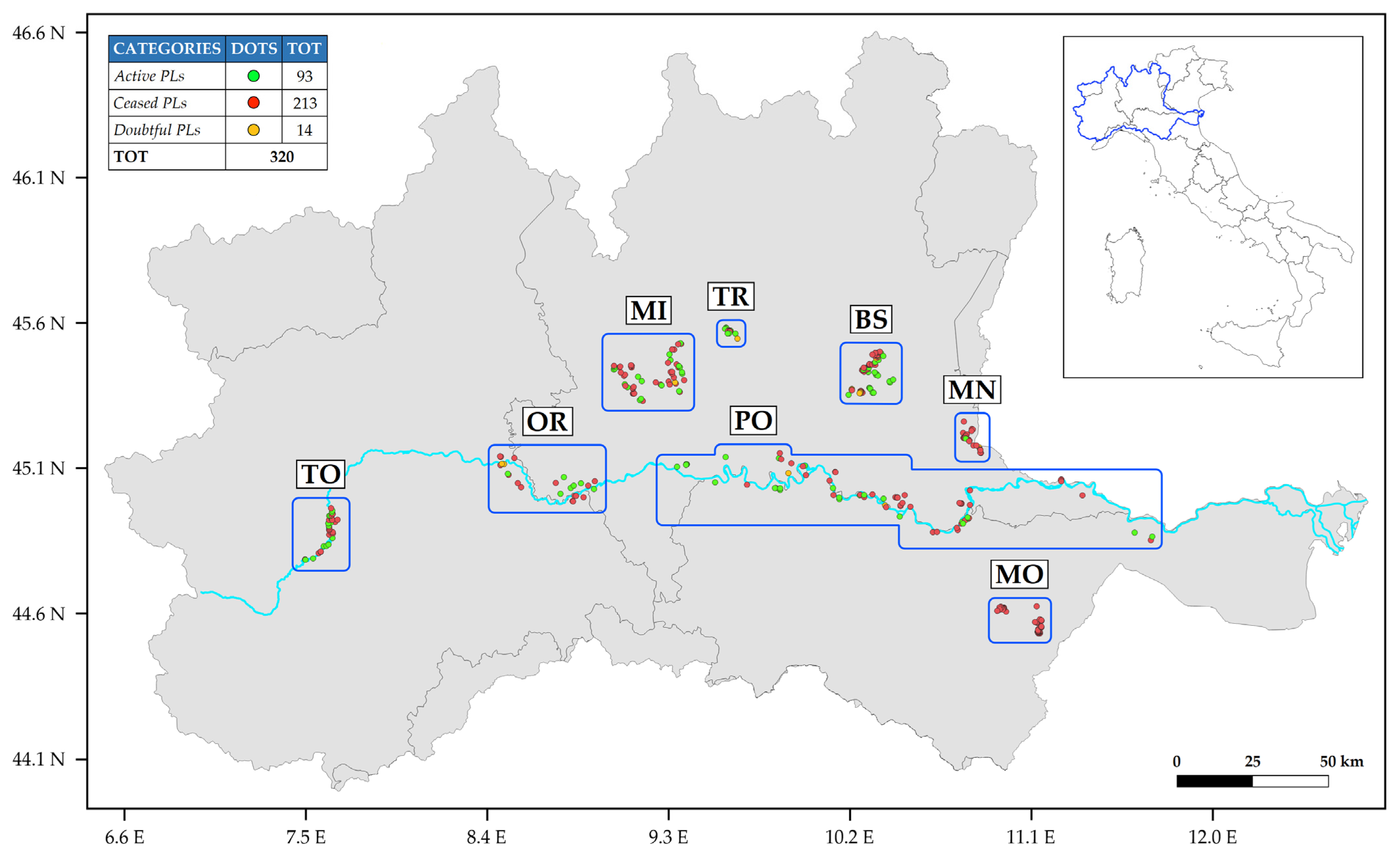
2.1. Study Area

The Po River basin extends around one of the largest rivers in the Mediterranean Sea and the longest river in Italy. The Po River is 652 km long and its basin covers approximately 74,000 km², of which ~71,000 km² are in Italy. In terms of water resources, the Po River (with an average annual flow of 1540 m³ s⁻¹ which has been gradually decreasing since the 21st century) is overexploited for irrigation, hydropower generation, and domestic purposes [82,83]. The Po River basin represents a key territory for the economy of the entire country; in fact, economic activities within it account for about 40% of Italy’s annual GDP [84,85]. In particular, the Po River basin contributes to about 60% of national sand and gravel production. The climax of this sector occurred from the post-World War II period until the 1980s, during which great amounts of inert materials were extracted directly from the riverbed to support post-war reconstruction, causing its gradual lowering [86]. Once the severity of the river alteration was felt, mining activity was moved to the floodplain, leading to the creation of numerous PLs. For more details regarding water resources and quarrying activities in the Po River basin, see [1].

In the Po River basin, 1580 PLs have been identified, of which 338 were still active in 2021 [1]. These PLs differ in location (isolated, in proximity to or connected to a river), size (<1 to 52 ha), and quarrying activity (active or ceased). For more details regarding identification and classification of PLs see [1].

For this study, a large subsample of PLs (320, both active and ceased) located in eight geographical areas within the basin was selected (Figure 1): Turin (TO), Po and Orba River Park (OR), Milan (MI), Trezzo sull’Adda (TR), Brescia (BS), Mantua (MN), Modena (MO), and along the Po River shaft (PO). These areas were selected because they are spatially well-distributed and representative of different land uses [1]. In each of these geographic areas, the density of PLs is high and consequently they exhibit a high degree of heterogeneity and well represent the entire basin.

2.2. The Processing of Satellite Images

Considering the wide time range used for this study (1990–2021), three different satellites were used: Landsat-5 (L5), Landsat-7 (L7) and Sentinel-2 (S2). The L5 and L7 belong to the Landsat constellation, and mount onboard TM (Thematic Mapper) and ETM+ (Enhanced Thematic Mapper) sensors, respectively. They are characterised by a spatial resolution of 30 m, a revisit time of about 16 days and 5 bands in the VIS-SWIR (Visible-Short Wavelength InfraRed) domain. The S2 mission, on the other hand, comprises two polar satellites (S2A and S2B), placed on the same orbit, but offset 180° from each other, allowing a revisit time of about 5 days. They mount onboard MultiSpectral Instrument (MSI) sensors, characterised by three different spatial resolutions (10, 20 and 60 m) and 13 bands in the VIS-SWIR.

All satellite images were downloaded as Level-1 (L1, i.e., not atmospherically corrected) from the following portals: https://catalogue.onda-dias.eu/catalogue/ (accessed on 1 October 2023) and https://earthexplorer.usgs.gov/ (accessed on 1 October 2023). All S2 images were resampled to the same spatial resolution (10 m). The years considered are listed in Table S1 and for each year, when available, six images were downloaded. Since there is no specific protocol for SPM concentration, we followed the protocol proposed by [87] for sampling lake phytoplankton, according to the European Water Framework Directive (WFD): winter (1 January–20 March), spring (1 April–15 May), spring-summer (16 May–15 June), summer (1 July–31 August), summer-autumn (1 September–1 October) and autumn (2 October–31 November). A total of 375 satellite images divided into the eight subsample areas were downloaded, and these images were free of clouds and other radiometric problems (e.g., sunglint).

ACOLITE v.2022 [88,89] was used to atmospherically correct satellite images and to obtain SPM concentration maps. ACOLITE is a neural network that groups atmospheric correction algorithms and allows users to derive different water quality parameters from Rrs values. In addition, it is particularly suitable for the analysis of turbid and small inland water bodies. ACOLITE requires L1 satellite images as inputs and can mask all water pixels autonomously. The atmospheric correction algorithm used was Dark Spectrum Fitting (DSF), which is able to estimate Aerosol Optical Depth at 550 nm (AOD₅₅₀) from dark targets, while the algorithms used to estimate SPM concentration were: SPM_Nechad2010 (for Landsat images), adjusted with the in situ data specific to our case studies, and the SPM_Nechad2016 (for S2 images). The former was proposed by [46], while the latter was recalibrated in 2016 specifically for S2 images. Both exploit the spectral characteristics of the red band (630–690 nm). For more information regarding the two algorithms, see [46].

2.3. Field Campaigns and Validation

To validate SPM concentration maps obtained by processing Landsat images with ACOLITE code, we used SPM concentration data collected by the University of Parma from 1993 to 2013. To this aim, all cloud-free Landsat images with a maximum discrepancy of two days from in situ sampling were downloaded, totalling 76 images. To validate S2 data, we carried out seven specific field campaigns (11 April 2022, 13 April 2022, 20 June 2022, 27 June 2022, 13 September 2022, 28 September 2022, and 15 June 2023) in PLs located in the PO area between 2022 and 2023 (Table S2).

During these field campaigns, water samples were collected, and spectral signatures (Rrs) were acquired at the same sites. Water samples were filtered with Whatman GF/F fibre filters and used to determine gravimetrically the SPM concentration according to [90]. Dry filters where subsequently incinerated in the muffle at 450 °C for 4 h to obtain inorganic and organic fractions of the particulate. Reflectance measurements were collected using the handheld spectrometer WISP-3 [91] produced by Water Insight. The instrument is designed for water quality studies and can be used for the optical validation of satellite data. The optical range is from 400 to 800 nm, with a bandwidth (full width half maximum) of ~4.9 nm and is able to simultaneously measure water and sky radiances at 42° to the nadir (L_u and L_sky, respectively) and downwelling irradiance (E_d), using three different optics and appropriate geometry. Together, these three optics can be used to obtain the Rrs of the water surface. All measurements (5 replicates for every single station) were taken away from the shoreline to avoid any influence of the bottom on the radiometric measurements; in addition, measurements were taken at an azimuth angle of ~135° to the sun to avoid any sunglint effects.

To compare the satellite data with in situ data, Regions of Interest (ROIs) (3 × 3 pixels) centred around the sampling site were created and the mean value was extracted for both SPM and Rrs; afterward, a series of descriptive statistics were calculated to assess their consistency. In detail, the determination coefficient (R²), Mean Absolute Error (MAE), Root Mean Square Error (RMSE) and Mean Absolute Percentage Error (MAPE) were calculated for both parameters. In addition, for spectral signatures only, the Spectral Angle (SA) was also calculated, which was used to determine how similar the shape of satellite spectra is to in situ data [92,93]. The metrics used were computed as follows:

$${\mathrm{R}}^2=1-\frac{{\sum }_{\mathrm{i}=1}^{\mathrm{n}}\left({\mathrm{x}}_{\mathrm{i}}-{\mathrm{y}}_{\mathrm{i}}\right)}{{\sum }_{\mathrm{i}=1}^{\mathrm{n}}{\left({\mathrm{x}}_{\mathrm{i}}-{\overline{\mathrm{x}}}_{\mathrm{i}}\right)}^2}$$

(1)

$$\mathrm{M}\mathrm{A}\mathrm{E}=\frac{{\sum }_{\mathrm{i}=1}^{\mathrm{n}}\left|{\mathrm{x}}_{\mathrm{i}}-{\mathrm{y}}_{\mathrm{i}}\right|}{\mathrm{n}}$$

(2)

$$\mathrm{R}\mathrm{M}\mathrm{S}\mathrm{E}=\sqrt{\frac{{\sum }_{\mathrm{i}=1}^{\mathrm{n}}{\left({\mathrm{x}}_{\mathrm{i}}-{\mathrm{y}}_{\mathrm{i}}\right)}^2}{\mathrm{n}}}$$

(3)

$$\mathrm{M}\mathrm{A}\mathrm{P}\mathrm{E}=\mathrm{m}\mathrm{e}\mathrm{d}\mathrm{i}\mathrm{a}\mathrm{n}\left(\left|\frac{{\mathrm{y}}_{\mathrm{i}}-{\mathrm{x}}_{\mathrm{i}}}{{\mathrm{x}}_{\mathrm{i}}}\right|100\%\right),\mathrm{i}=1,\dots \mathrm{N}$$

(4)

$$\mathrm{S}\mathrm{A}={\mathrm{c}\mathrm{o}\mathrm{s}}^{-1}\frac{{\sum }_{\mathrm{i}=1}^{\mathrm{n}}{\mathrm{x}}_{\mathrm{i}}{\mathrm{y}}_{\mathrm{i}}}{\sqrt{{\sum }_{\mathrm{i}=1}^{\mathrm{n}}{\mathrm{y}}_{\mathrm{i}}^2}\sqrt{{\sum }_{\mathrm{i}=1}^{\mathrm{n}}{\mathrm{x}}_{\mathrm{i}}^2}}$$

(5)

where $x_i$ are the in situ values, ${\overline{x}}_i$ is the mean of the in situ values and $y_i$ are the values derived from satellite images.

In order to compare the spectral signatures acquired in situ (hyperspectral) with the spectral signatures of S2 (multispectral), a resampling of the hyperspectral signatures was performed based on spectral characteristics of S2. In particular, the higher spectral resolution of WISP data were spectrally resampled according to the full width half maximum (FWHM) of S2 data.

2.4. Pit Lakes Analysis

The identification of water pixels by ACOLITE is not always accurate because the pixels located at the water–land interface, which could lead to an overestimation of SPM concentrations, are often retained. For this reason, ACOLITE products were overlaid on the true colour images in order to verify the effective removal of terrestrial pixels and clouds. After that, starting from the ACOLITE water mask, all pixels located near the shorelines were manually removed. In addition, spectral signatures were examined for outliers within the water pixels. Once the ROIs were created, they were used to extract SPM concentration and Rrs values in the Visible domain, which were needed to obtain the λ_dom (water colour) via the Forel-Ule index [63]. More information on the procedure to obtain the λ_dom from Landsat and S2 images can be found in [63]. Finally, all outliers characterised by negative or excessively high values, often due to the presence of dredges in the middle of active PLs, were manually removed from these maps. Once the SPM concentrations were extracted from the PLs of all available images, the temporal trends of each lake and the average SPM concentration of each subsample area were calculated.

PLs were also divided into various thematic groups, with the purpose of understanding whether SPM concentration and λ_dom changed according to lake location, size, season (according to WFD protocol) and quarrying activity. Based on location, PLs were divided into three categories: isolated, in proximity to (at most 500 m away from a watercourse) or connected to a river. Based on dimension, they were divided into: small (<5 ha), medium (5–10 ha) and large (>10 ha). Based on season, the WFD protocol was followed, while based on quarrying activity, they were divided into: active and ceased. The Mann–Whitney and Kruskal–Wallis nonparametric tests were performed to assess whether there were significant differences in SPM and λ_dom among the categories that compose each thematic group.

To specifically assess the impact of quarrying activity on the evolution of the water quality of PLs, two types of analysis were conducted on a restricted number of PLs. The first involved the analysis of temporal trends of SPM concentration in 13 PLs whose quarrying activity ceased during the observed period (1990–2021). Specifically, the mean SPM concentrations before and after the end of quarrying activity was calculated for the 13 lakes, considering all available images. For this analysis, the cumulative precipitation during the seven days prior to the date of satellite acquisition was measured to understand the influence of this meteorological factor. The wind was not considered because the PLs examined were characterised by extensive areas of riparian vegetation in their surroundings (on average, 80% of the perimeter of those PLs were covered by vegetation). The second analysis concerned two adjacent PLs located in the MI area: one whose quarrying activity had ceased (MI-30), and the other which was characterised instead by frequent quarrying episodes (MI-31). For this analysis, 27 S2 images acquired during quarrying events were downloaded and processed with ACOLITE in order to obtain SPM concentration maps.

3. Results

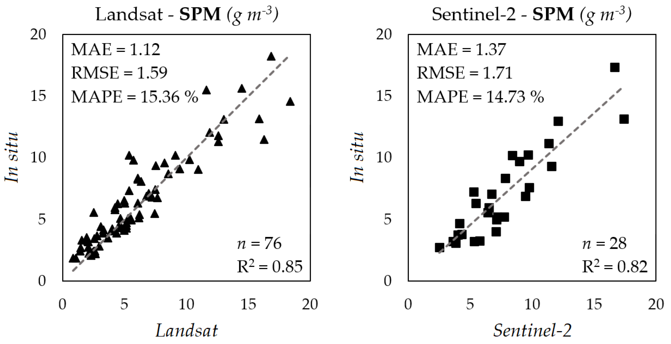
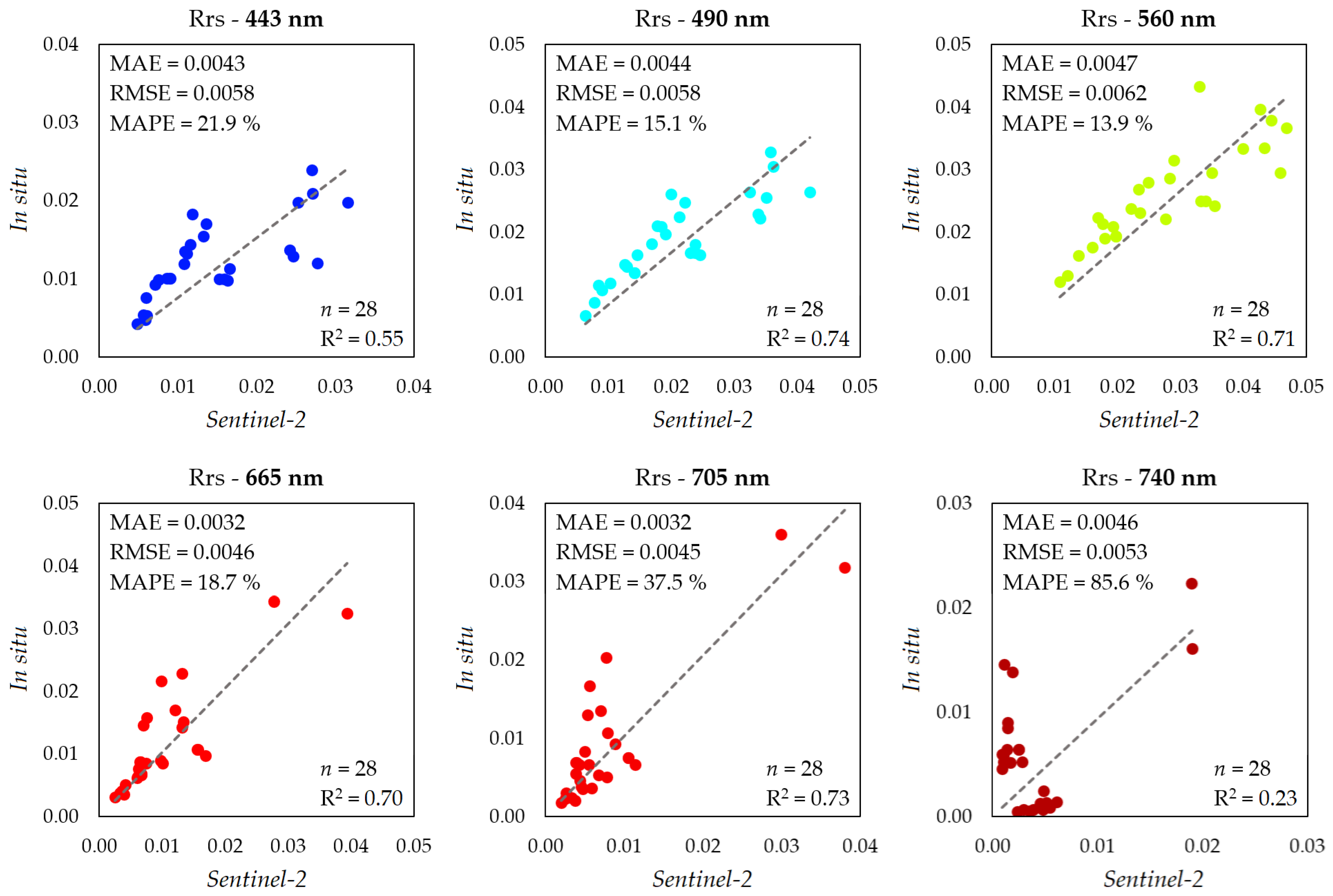
3.1. Satellite Data Validation

The statistical comparison between the SPM concentrations obtained in situ and those derived from satellite images showed that there is a very strong correlation between both the data derived from Landsat images (R² = 0.85) and those from S2 images (R² = 0.82). However, it appeared that the SPM_Nechad2010 algorithm applied to the Landsat images overestimated the SPM concentration; consequently, two calibration coefficients were applied, one for the L5 and one for the L7 data, calculated on the basis of the slope of the regression lines. In both scatterplots, we removed a comparison related to a very turbid lake because, although there was a strong correlation between the in situ and satellite data, they distorted the R² values, over-improving them.

The comparison of the spectral signatures obtained using WISP-3 and those derived from ACOLITE showed that there is a strong correlation in the visible spectrum, while some issues emerge in the NIR domain (a slight overestimation of satellite values). This overestimation is not impactful for this work, since the algorithms for estimating the SPM concentration were based on the red band (630–690 nm), while the calculation of the λ_dom was based on the visible bands. Furthermore, the accuracy of the spectral signatures obtained through ACOLITE is also justified by the low SA values obtained for the 28 comparisons performed (10.8° ± 5.7°). The graphs for the statistical metrics are shown in Figure 2 and Figure 3.

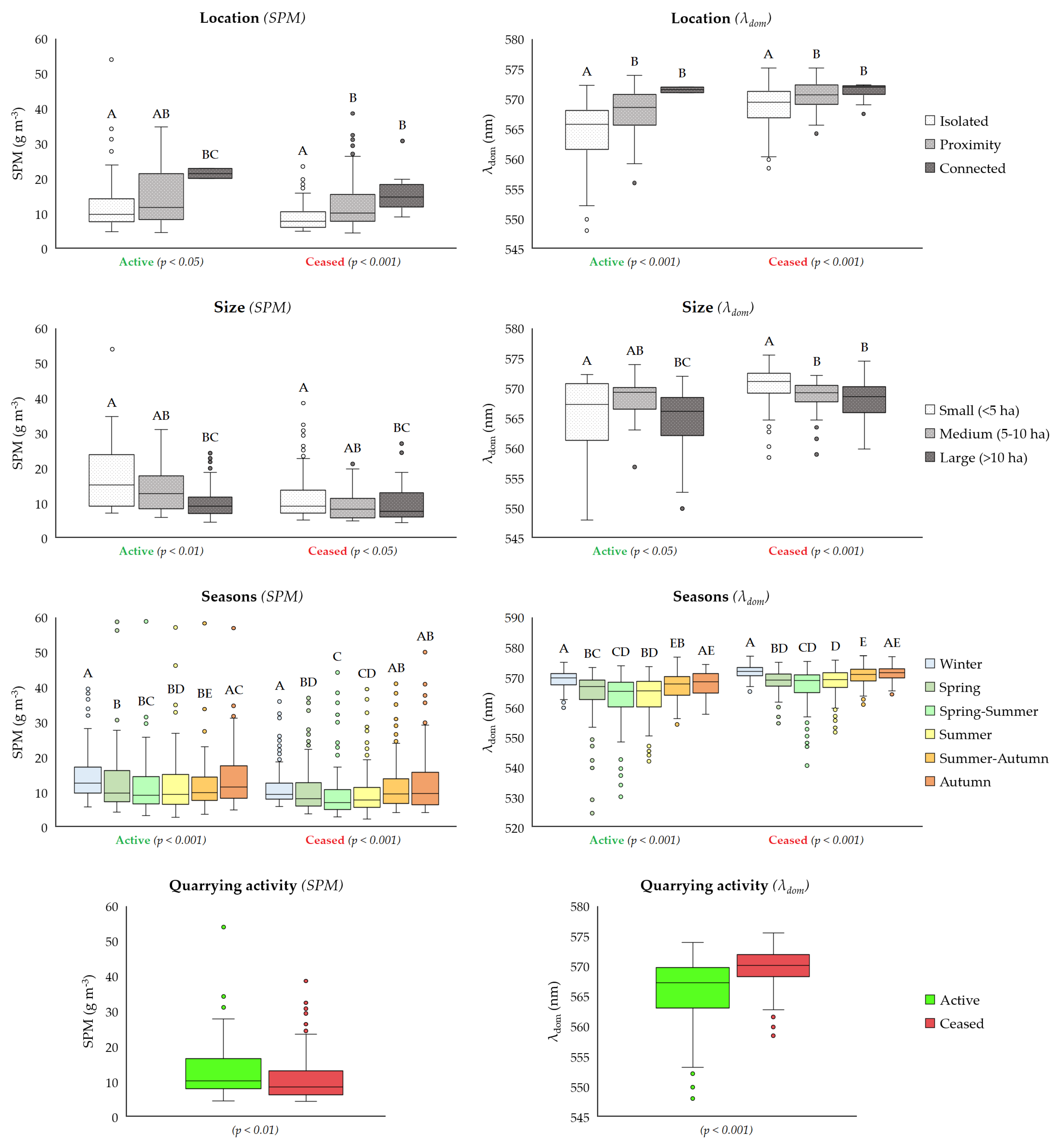
3.2. SPM Concentration and Water Colour

Figure 4 shows the mean SPM concentration and the mean λ_dom (1990–2021) for all PLs of the subsample investigated. SPM values range from 1 to 88 g m³, while λ_dom range from 480 to 589 nm. The PLs with the highest mean SPM concentrations are located along the Po River (especially in OR and PO areas) and more generally near rivers. For mean λ_dom, the pattern is also similar, although it is less pronounced than that of SPM concentration. In fact, PLs with high mean λ_dom are mainly located near rivers, although they are also present in other areas (e.g., MI area).

Based on the PLs’ locations, the analysis shows that those connected to a river (active: 21.4 ± 2.0 g m⁻³; ceased: 15.7 ± 5.9 g m⁻³) are characterised by higher mean SPM concentrations than both PLs located in proximity of a watercourse (active: 14.5 ± 7.9 g m⁻³; ceased: 12.8 ± 7.4 g m⁻³) and isolated ones (active: 12.4 ± 8.2 g m⁻³; ceased: 8.9 ± 3.7 g m⁻³), for both active and ceased PLs. The same result also emerges for the mean λ_dom. Based instead on size, smaller PLs (active: 18.2 ± 11.5 g m⁻³; ceased: 11.4 ± 6.6 g m⁻³) have the highest mean SPM concentrations compared to medium (active: 14.3 ± 7.2 g m⁻³; ceased: 9.3 ± 4.2 g m⁻³) and large lakes (active: 10.7 ± 5.3 g m⁻³; ceased: 9.7 ± 5.1 g m⁻³). In this case, the difference between the three categories is more pronounced for active PLs than for ceased ones. The mean λ_dom follows the same pattern only for ceased PLs (571 ± 3, 569 ± 3, 568 ± 3 nm, respectively), while smaller active PLs are characterised by lower mean λ_dom than medium sized PLs (565 ± 7, 568 ± 4, 565 ± 5 nm, respectively). Seasonal comparison shows the same trend for both SPM concentration and λ_dom: higher values in winter gradually decrease until spring–summer, then increase again. No differences are visible between active and ceased PLs. Finally, the comparison based on quarrying activity shows that active PLs (13.3 ± 8.2 g m⁻³) exhibit higher mean SPM concentration than ceased PLs (10.6 ± 5.9 g m⁻³); however, ceased PLs (570 ± 3 nm) show higher mean λ_dom than active PLs (566 ± 6 nm). All comparisons are shown in Figure 5, while the values divided into the eight subsample areas are reported in Tables S3 and S4.

By comparing the PLs characterised by low mean values of SPM and λ_dom (PLs _low) with the PLs characterised by high mean values of SPM and λ_dom (PLs _high), it was observed that the PLs _low are larger (mean: 12 ha) and older (and consequently deeper). These PLs are predominantly isolated and consistently exhibit lower mean SPM concentrations compared to the overall mean of the subsample area where they are located. On the other hand, PLs _high are smaller (mean: 5 ha) and younger (and consequently shallower). They are predominantly located in proximity or directly connected to a river, and consistently display higher mean SPM concentrations compared to the overall mean of the subsample area in which they are located.

3.3. The Impact of Quarrying Activity and Precipitation

Table 1. SPM concentrations (mean ± st.dev.) before and after the end of quarrying activity for the 13 pit lakes (PLs) examined (observation period: 1990–2021).

PLs	Coordinates	Quarrying Activity	Before (g m−3)	After (g m−3)	SPM Reduction (%)
OR-4	45.161294N; 8.548939E	1995–2012	9.7 ± 4.4	5.5 ± 3.6	−43
OR-22	45.031655N; 8.873921E	2005–2008	18.1 ± 7.7	7.4 ± 3.9	−59
OR-25	45.070040N; 8.895304E	2003–2007	19.8 ± 6.8	7.7 ± 3.2	−61
BS-11	45.378769N; 10.181337E	2006–2012	17.3 ± 7.8	8.5 ± 4.8	−51
BS-42	45.464501N; 10.250156E	<1990–2005	12.5 ± 5.7	5.8 ± 2.5	−54
BS-49	45.491103N; 10.263158E	<1990–2007	11.6 ± 6.0	6.6 ± 3.2	−43
MN-2	45.245806N; 10.699478E	1999–2007	14.3 ± 7.9	7.3 ± 2.8	−49
MO-5	44.673111N; 10.817644E	2006–2014	20.4 ± 6.9	5.9 ± 2.6	−71
PO-9	45.059638N; 9.775130E	<1990–2009	15.0 ± 8.1	7.3 ± 3.0	−51
PO-14	45.155322N; 9.801703E	2002–2012	19.4 ± 12.9	5.5 ± 1.9	−72
PO-17	45.141368N; 9.849019E	2002–2012	16.9 ± 7.2	8.3 ± 3.2	−51
PO-54	44.911351N; 10.623380E	1998–2012	20.4 ± 10.1	10.4 ± 5.4	−49
PO-77	44.861300N; 11.524369E	<1990–2008	14.0 ± 5.9	7.0 ± 3.3	−50

shows the mean SPM concentrations of the 13 PLs before and after the cessation of quarrying activity (Figures S1–S5). The results show that the mean SPM concentration decreases from a minimum of 43% to a maximum of 72% (a mean reduction of 54%).

A clear correlation between SPM concentration and cumulative precipitation was not found for the 13 PLs analysed. For these comparisons, we exclusively considered values obtained after the ending of the quarrying activity. This approach ensured the elimination of any variability introduced by the resuspension associated with dredging.

Figure 6 shows the SPM concentration of PLs MI-30 (ceased) and MI-31 (active) during some quarrying events. The results show that MI-31 is consistently characterised by higher SPM concentrations than MI-30, especially in the southern part where the dredge is located. In addition, it is evident how the SPM peak located in the excavation area moved and extended rapidly within a few days to the entire lake (e.g.,16 June 2018 to 21 June 2018, 9 September 2019 to 14 September 2019, 10 June 2021 to 15 June 2021).

4. Discussion

4.1. The Reliability of Remote Sensing for PLs’ Water Quality Assessments

Satellites used for land monitoring, such as Landsat and Sentinel-2, provide images characterised by high spatial resolution that enable the assessment of water quality parameters. In particular, recent studies have corroborated the capabilities of such satellites in monitoring inland waters and small lakes [18,94,95,96,97,98]. This success can be attributed to the increase in the average revisit interval, which has resulted in a concomitant increase in the number of cloud-free images. Such an abundance of data, therefore, allows a near real-time monitoring of such dynamic environments.

In this study, we conducted an in-depth analysis of the reliability of Landsat-5, Landsat-7 and Sentinel-2 satellites in assessing the physical and optical properties of PLs, focusing on the estimation of SPM concentration and λ_dom. Our approach included the comparison of SPM concentration data obtained in situ by limnological techniques with those retrieved through the use of the neural network ACOLITE on satellite data. The results of this comparison revealed a remarkable agreement; however, the SPM_Nechad2010 algorithm employed for the Landsat images showed a tendency to overestimate SPM concentrations. It was necessary to correct this overestimation by a recalibration process based on the reference data obtained in situ. The validation was mainly focused on PLs characterised by SPM concentrations below 20 g m⁻³, due to a logistic constrain that did not allow the access to many PLs for field measurements. However, although only a few data were available for PLs with particularly high SPM concentrations, the agreement between in situ and satellite values was very strong. Nevertheless, these data were not included in the main validation step, as they would have distorted the scatterplots (Figure 2), over-enhancing the coefficient of determination (R²). In the future, it would be appropriate to find accessible PLs with SPM concentrations above 20 g m⁻³. This would allow a more complete and detailed validation of the performance of the ACOLITE algorithm in environments characterised by such levels of SPM concentration. Moreover, it would be interesting to identify a few sample lakes and analyse their temporal evolution in detail through the integration of S2 data with products derived from, for example, Landsat-8 and Landsat-9 images, in order to avoid temporal gaps between data.

In addition to the SPM concentration, we also performed a comparison of the Rrs spectral signatures, obtained by the atmospheric correction of S2 images through ACOLITE, with those acquired through the Water Insight spectrometer WISP-3. This spectral parameter is essential for the calculation of λ_dom, and consequently, a robust agreement between the values obtained in situ and those detected by satellites is crucial. The comparison reveals strong agreement in the visible domain (400–700 nm), while some discrepancies were found in the NIR domain (a slight overestimation of satellite values). Specifically, the 740 nm band showed very good effectiveness for turbid waters, as the presence of high SPM concentrations increases reflectance levels in both the red and NIR domains. However, this band is not as effective in clearer waters, where reflectance values should tend to zero. This phenomenon could result from an error in atmospheric correction due to the intrinsic properties of water in the infrared domain [99,100]. This overestimation does not have a significant impact on our investigation, since the two algorithms used to estimate SPM concentrations (SPM_Nechad2010 and SPM_Nechad2016) were based on the red band (630–690 nm), while the calculation of λ_dom was based exclusively on the visible bands. More generally, the strong agreement between the spectral signatures collected in situ and those obtained from satellite data was confirmed by the low values obtained from the calculation of the SA statistical index (10.8° ± 5.7°).

4.2. The Assessment of PLs’ Water Quality

The use of a combined approach between Landsat and Sentinel-2 satellite images allowed for the estimation of the mean SPM concentration and mean λ_dom for each PL over a three-decade period (1990–2021). Most of the challenges in inland water observations are due to their optical complexity. These aquatic ecosystems can be a mixture of optically shallow and deep waters, with gradients of oligotrophic to hypertrophic productive waters and clear to turbid conditions. Hence, a large range in optical absorption and backscattering resulting in high optical variability can be found among and within lakes. This creates a challenge for algorithms applied to optical remote sensing for water-quality monitoring. Furthermore, another challenge is performing atmospheric corrections over such variable aquatic ecosystems, as their complexity requires different approaches than those for land and ocean applications.

The results of this temporal analysis revealed that the PLs with the highest mean SPM concentrations and highest mean λ_dom are located along the Po River (especially in the OR and PO areas) and, in general, near waterways and rivers. This finding is further confirmed through the subdivision of PLs into thematic groups; in fact, PLs connected to a river and those located in their proximity exhibited higher mean SPM concentrations and mean λ_dom than isolated PLs. These PLs are fed by river waters and, especially during flood periods, receive a large amount of suspended solids and nutrients that can lead to a higher trophic state [9]. Recent studies have shown that, as a consequence of climate change, periods of prolonged drought followed by short periods of flooding after intense precipitation are becoming more frequent and intense in the Po River basin [83]. Thus, our results suggest that there is a significant potential for climate change to affect the water quality of PLs, particularly those connected to rivers, with prolonged periods of higher transparency during droughts and more turbid waters following flood events.

Focusing on quarrying activity, it turned out, as might be expected, that active PLs are characterised by a higher mean SPM concentration than ceased PLs. This is mainly due to the mechanical action of the dredgers, which collect inert materials from the lake bottom and cause considerable resuspension of bottom sediments and stirring of suspended material. On the other hand, the mean λ_dom analysis shows that the ceased PLs show a higher mean λ_dom than the active PLs. Specifically, ceased PLs tend more toward a green-yellow colour, a feature attributable to the moderate presence of phytoplankton and Coloured Dissolved Organic Matter (CDOM). In fact, the absence of turbulence caused by dredges may contribute to greater water clarity, allowing sunlight to penetrate deeper and potentially promoting more algal particle growth. In addition, the high cover of riparian vegetation in the surroundings of the ceased PLs could result in an increased concentration of CDOM, via inputs of allochthonous dissolved organic matter [101,102].

The division of PLs according to size revealed that small lakes (<5 ha) on average have higher SPM concentrations than their larger counterparts. This trend is more pronounced in PLs that are still active, while it tends to diminish in those that have ceased the quarrying activity. The explanation for this phenomenon may lie in the fact that, in smaller active PLs, quarrying activity has only recently started. As a result, such lakes are generally shallow and subject to the mechanical action of dredges, and to wind and fish action. These phenomena can resuspend lake sediment from the bottom, causing a drastic increase in SPM concentrations. The same trend is also reflected in the analysis of the mean λ_dom in ceased PLs, while for active PLs, the results show that small-sized PLs are characterised by a lower λ_dom than medium-sized PLs. This result could be attributed to the sparseness or absence of riparian vegetation in small-sized active PLs. In fact, the presence of riparian vegetation may lead to the introduction of organic debris into the waters, which, once dissolved, may contribute to increases in the λ_dom.

Finally, the increase in SPM concentration during the winter and autumn periods can be attributed to water mixing, increased wind and rainfall, and a reduction in riparian vegetation; factors that promote the input of particulate material from outside. In addition, more organic debris may flow in lake waters during these periods, leading to an increase in CDOM. On the other hand, the green hue of the waters, predominant in the spring and summer months, may be explained by algal blooms, caused by increased nutrients reaching the lake from agricultural fields, associated with higher temperatures.

4.3. The Impact of Quarrying Activity and Precipitation

Quarrying activity has been proven to have a considerable impact on PLs. For example, the turbulence generated within the water column disrupts thermal stratification and resuspends significant amounts of sediment, exerting a significant influence on the lake’s planktonic community [103,104,105]. At the same time, sediment resuspension contributes to increased turbidity in the water, resulting in decreased sunlight penetration. This phenomenon, in addition to reducing the amount of light available to phytoplankton, influences macrophyte communities that may establish along banks characterised by gentle slopes. Such communities play a crucial role in maintaining high water quality standards [106], as well as providing habitats and food sources for numerous aquatic organisms [7,8].

The characteristics of the MSI sensor installed onboard the S2 have been proven suitable for analysing the impact of quarrying activity on the SPM concentration of PLs. This suitability extends to both the long-term, allowing for the evaluation of temporal trends in SPM concentrations before and after the cessation of quarrying activities, and the short-term, allowing for the detection of recurring and episodic turbidity events in specific PLs that occur at small spatio-temporal scales. However, despite a high spatial resolution and a short revisit time, the extent of some small, newly formed pit lakes and the presence of clouds at specific periods of the year may limit the observation of short, punctual quarrying episodes.

As was to be expected, the end of quarrying activity led to a marked decrease in SPM concentrations in all of the PLs examined (a mean reduction of 54%), mainly due to the cessation of the mechanical sediment-stirring action carried out by the dredges. However, even once quarrying activity was over, no direct correlation emerged between SPM concentrations and total precipitation, as might have been expected. This could depend on multiple factors, including the actual location of the weather station relative to the lake and the time scale adopted, as soil erosion responds not only to the total amount of rainfall but also to rainfall intensity. In our perspective, it would be interesting to identify a weather station near a lake and consider a change in the time interval considered for the total precipitation. A plausible hypothesis is that within the total precipitation, rainfall that occurs shortly after the satellite image acquisition may have a greater influence than rainfall that occurs days later. Moreover, there is a complex relation between precipitation intensity, plant biomass and composition and erosion [107] that could influence water quality. This analysis is beyond the scope of this work but, given the observed changes in land cover due to climate change and anthropogenic activities observed in the Po river watershed [108], the approach adopted in this work could be useful in the future for understanding the consequences of climate change and directing anthropic activity on the water quality of PLs.

An additional finding from this research indicates that the resuspension action actuated by the dredges is not confined to a single well-defined point. On the contrary, the increase in the SPM concentration found at the sampling point spread gradually throughout the entire lake over the course of a few days (potentially even more rapidly, given the frequency of the revisiting of S2, which occurred approximately every 5 days).

5. Conclusions

This research confirmed the reliability of Landsat and Sentinel-2 satellites in performing a basin-scale assessment of SPM and λ_dom concentrations in small, dynamic inland waters such as PLs. The approach adopted to quantify these two parameters allowed a comprehensive and in-depth assessment of the quality status of these ecosystems over three decades (1990 to 2021). The spatial and spectral characteristics of these satellites opened up new perspectives in the study of these lakes, which were otherwise inaccessible using traditional limnological techniques.

The key results include that the water quality status in these lakes depends on multiple factors, including their location and size. In fact, it was found that the lakes with a poor water quality status (based on both SPM concentration and λ_dom) were those of small sizes, often located near or directly connected to rivers. In addition, quarrying activity appears to have a significant impact on PLs, as it has been demonstrated that the end of such activities results in a marked decrease in SPM concentrations (a mean reduction of 54%). Inversely, the extraction of inert materials from the lake bottom causes an increase in SPM concentrations, an effect that propagates rapidly throughout the water body from the point of extraction. In this regard, the Sentinel-2 satellite has proven to be a reliable tool for detecting these episodic or recurrent events in a dynamic context.

A significant future step in the study of these aquatic ecosystems could be the installation of fixed instruments for collecting continuous spectral measurements to estimate SPM concentrations. This type of approach would allow for further insight into the study of water quality through continuous measurements that could overcome the limitations of satellite remote sensing, such as revisit time and cloud cover. The integration of in situ and remote data both radiometric and limnological combines synergistically to provide insight into waterbody bio-geochemistry, which can be extended over time, allowing their genesis and evolution to be explored.

References

1. Ghirardi, N.; Bresciani, M.; Pinardi, M.; Nizzoli, D.; Viaroli, P. Pit lakes from gravel and sand quarrying in the Po River basin: An opportunity for riverscape rehabilitation and ecosystem services improvement. Ecol. Eng. 2023, 196, 107103. [Google Scholar] [CrossRef]
2. Peckenham, J.M.; Thornton, T.; Whalen, B. Sand and gravel mining: Effects on ground water resources in Hancock county, Maine, USA. Environ. Geol. 2009, 56, 1103–1114. [Google Scholar] [CrossRef]
3. Weilhartner, A.; Muellegger, C.; Kainz, M.; Mathieu, F.; Hofmann, T.; Battin, T.J. Gravel pit lake ecosystems reduce nitrate and phosphate concentrations in the outflowing groundwater. Sci. Total Environ. 2012, 420, 222–228. [Google Scholar] [CrossRef] [PubMed]
4. Muellegger, C.; Weilhartner, A.; Battin, T.J.; Hofmann, T. Positive and negative impacts of five Austrian gravel pit lakes on groundwater quality. Sci. Total Environ. 2013, 443, 14–23. [Google Scholar] [CrossRef] [PubMed]
5. Blanchette, M.L.; Lund, M.A. Pit lakes are a global legacy of mining: An integrated approach to achieving sustainable ecosystems and value for communities. Curr. Opin. Environ. Sustain. 2016, 23, 28–34. [Google Scholar] [CrossRef]
6. McCullough, C.D.; Lund, M.A. Pit lakes: Benefit or bane to companies, communities and the environment. In Proceedings of the Proc (CD), Goldfields Environmental Management Group Workshop on Environmental Management, Kalgoorlie-Boulder, Australia, 24–26 May 2006. [Google Scholar]
7. Mollema, P.N.; Antonellini, M. Water and (bio) chemical cycling in gravel pit lakes: A review and outlook. Earth Sci. Rev. 2016, 159, 247–270. [Google Scholar] [CrossRef]
8. Søndergaard, M.; Lauridsen, T.L.; Johansson, L.S.; Jeppesen, E. Gravel pit lakes in Denmark: Chemical and biological state. Sci. Total Environ. 2018, 612, 9–17. [Google Scholar] [CrossRef]
9. Nizzoli, D.; Welsh, D.T.; Viaroli, P. Denitrification and benthic metabolism in lowland pit lakes: The role of trophic conditions. Sci. Total Environ. 2020, 703, 134804. [Google Scholar] [CrossRef]
10. Kattner, E.; Schwarz, D.; Maier, G. Eutrophication of gravel pit lakes which are situated in close vicinity to the River Donau: Water and nutrient transport. Limnologica 2000, 30, 261–270. [Google Scholar] [CrossRef]
11. Nizzoli, D.; Welsh, D.T.; Longhi, D.; Viaroli, P. Influence of Potamogeton pectinatus and microphytobenthos on benthic metabolism, nutrient fluxes and denitrification in a freshwater littoral sediment in an agricultural landscape: N assimilation versus N removal. Hydrobiologia 2014, 737, 183–200. [Google Scholar] [CrossRef]
12. Kirk, J.T.O. Optical water quality, what does it mean and how should we measure it? JSTOR 1988, 60, 194–197. [Google Scholar]
13. Wang, S.; Li, J.; Zhang, W.; Cao, C.; Zhang, F.; Shen, Q.; Zhang, X.; Zhang, B. A dataset of remote-sensed Forel-Ule Index for global inland waters during 2000–2018. Sci. Data 2021, 8, 26. [Google Scholar] [CrossRef]
14. Pozdnyakov, D.; Shuchman, R.; Korosov, A.; Hatt, C. Operational algorithm for the retrieval of water quality in the Great Lakes. Remote Sens. Environ. 2005, 97, 352–370. [Google Scholar] [CrossRef]
15. Xing, Q.G.; Lou, M.J.; Chen, C.Q.; Shi, P. Using in situ and Satellite Hyperspectral Data to Estimate the Surface Suspended Sediments Concentrations in the Pearl River Estuary. IEEE J. Sel. Top. Appl. Earth Obs. Remote Sens. 2013, 6, 731–738. [Google Scholar] [CrossRef]
16. Doxaran, D.; Lamquin, N.; Park, Y.J.; Mazeran, C.; Ryu, J.H.; Wang, M.; Poteau, A. Retrieval of the Seawater Reflectance for Suspended Solids Monitoring in the East China Sea Using MODIS, MERIS and GOCI Satellite Data. Remote Sens. Environ. 2014, 146, 36–48. [Google Scholar] [CrossRef]
17. Chen, F.; Wu, G.; Wang, J.; He, J.; Wang, Y. A MODIS-Based Retrieval Model of Suspended Particulate Matter Concentration for the Two Largest Freshwater Lakes in China. Sustainability 2016, 8, 832. [Google Scholar] [CrossRef]
18. Liu, H.; Li, Q.; Shi, T.; Hu, S.; Wu, G.; Zhou, Q. Application of sentinel 2 MSI images to retrieve suspended particulate matter concentrations in Poyang Lake. Remote Sens. 2017, 9, 761. [Google Scholar] [CrossRef]
19. Zhao, X.; Zhao, J.; Zhang, H.; Zhou, F. Remote Sensing of Sub-Surface Suspended Sediment Concentration by Using the Range Bias of Green Surface Point of Airborne LiDAR Bathymetry. Remote Sens. 2018, 10, 681. [Google Scholar] [CrossRef]
20. Ciancia, E.; Campanelli, A.; Lacava, T.; Palombo, A.; Pascucci, S.; Pergola, N.; Pignatti, S.; Satriano, V.; Tramutoli, V. Modeling and multi-temporal characterization of total suspended matter by the combined use of Sentinel 2-MSI and Landsat 8- OLI data: The Pertusillo Lake case study (Italy). Remote Sens. 2020, 12, 2147. [Google Scholar] [CrossRef]
21. Jiang, D.; Matsushita, B.; Pahlevan, N.; Gurlin, D.; Lehmann, M.K.; Fichot, C.G.; Schalles, J.; Loisel, H.; Binding, C.; Zhang, Y.; et al. Remotely estimating total suspended solids concentration in clear to extremely turbid waters using a novel semi-analytical method. Remote Sens. Environ. 2021, 258, 112386. [Google Scholar] [CrossRef]
22. Walch, H.; Von der Kammer, F.; Hofmann, T. Freshwater suspended particulate matter—Key components and processes in floc formation and dynamics. Water Res. 2022, 220, 118655. [Google Scholar] [CrossRef]
23. Gernez, P.; Lafon, V.; Lerouxel, A.; Curti, C.; Lubac, B.; Cerisier, S.; Barillé, L. Toward Sentinel-2 High Resolution Remote Sensing of Suspended Particulate Matter in Very Turbid Waters: SPOT4 (Take5) Experiment in the Loire and Gironde Estuaries. Remote Sens. 2015, 7, 9507–9528. [Google Scholar] [CrossRef]
24. Hou, X.; Feng, L.; Duan, H.; Chen, X.; Sun, D.; Shi, K. Fifteen-year monitoring of the turbidity dynamics in large lakes and reservoirs in the middle and lower basin of the Yangtze River, China. Remote Sens. Environ. 2017, 190, 107–121. [Google Scholar] [CrossRef]
25. Moore, K.A.; Wetzel, R.L.; Orth, R.J. Seasonal pulses of turbidity and their relations to eelgrass (Zostera marina L.) survival in an estuary. J. Exp. Mar. Biol. Ecol. 1997, 215, 115–134. [Google Scholar] [CrossRef]
26. Doxaran, D.; Froidefond, J.M.; Lavender, S.; Castaing, P. Spectral signature of highly turbid waters: Application with SPOT data to quantify suspended particulate matter concentrations. Remote Sens. Environ. 2002, 81, 149–161. [Google Scholar] [CrossRef]
27. Havens, K.E. Submerged aquatic vegetation correlations with depth and light attenuating materials in a shallow subtropical lake. Hydrobiologia 2003, 493, 173–186. [Google Scholar] [CrossRef]
28. Guildford, S.J.; Bootsma, H.A.; Taylor, W.D.; Hecky, R.E. High variability of phytoplankton photosynthesis in response to environmental forcing in oligotrophic Lake Malawi/Nyasa. J. Great Lakes Res. 2007, 33, 170–185. [Google Scholar] [CrossRef]
29. Zhu, M.Y.; Zhu, G.W.; Li, W.; Zhang, Y.L.; Zhao, L.L.; Gu, Z. Estimation of the Algal-Available Phosphorus Pool in Sediments of a Large, Shallow Eutrophic Lake (Taihu, China) Using Profiled SMT Fractional Analysis. Environ. Pollut. 2013, 173, 216–223. [Google Scholar] [CrossRef]
30. Ma, Y.; Song, K.; Wen, Z.; Liu, G.; Shang, Y.; Lyu, L.; Du, J.; Yang, Q.; Li, S.; Tao, H.; et al. Remote sensing of turbidity for lakes in northeast China using Sentinel-2 images with machine learning algorithms. IEEE J. Sel. Top. Appl. Earth Obs. Remote Sens. 2021, 14, 9132–9146. [Google Scholar] [CrossRef]
31. Wen, Z.; Wang, Q.; Liu, G.; Jacinthe, P.A.; Wang, X.; Lyu, L.; Tao, H.; Ma, Y.; Duan, H.; Shang, Y.; et al. Remote sensing of total suspended matter concentration in lakes across China using Landsat images and Google Earth Engine. ISPRS J. Photogramm. Remote Sens. 2022, 187, 61–78. [Google Scholar] [CrossRef]
32. Zhang, Y.; Shi, K.; Liu, X.; Zhou, Y.; Qin, B. Lake topography and wind waves determining seasonal-spatial dynamics of total suspended matter in turbid Lake Taihu, China: Assessment using long-term high-resolution MERIS data. PLoS ONE 2014, 9, e98055. [Google Scholar] [CrossRef] [PubMed]
33. Wu, G.; Cui, L.; Liu, L.; Chen, F.; Fei, T.; Liu, Y. Statistical model development and estimation of suspended particulate matter concentrations with Landsat 8 OLI images of Dongting Lake, China. Int. J. Remote Sens. 2015, 36, 343–360. [Google Scholar] [CrossRef]
34. Lebeuf, M.; Maltais, D.; Larouche, P.; Lavoie, D.; Scarratt, M. Recent distribution and temporal changes of suspended particulate matter in the st lawrence estuary, canada. Reg. Stud. Mar. Sci. 2019, 29, 2352–4855. [Google Scholar]
35. Bilotta, G.S.; Brazier, R.E. Understanding the influence of suspended solids on water quality and aquatic biota. Water Res. 2008, 42, 2849–2861. [Google Scholar] [CrossRef] [PubMed]
36. Williamson, T.N.; Crawford, C.G. Estimation of Suspended-Sediment Concentration From Total Suspended Solids and Turbidity Data for Kentucky; 1978–1995 1. JAWRA J. Am. Water Resour. Assoc. 2011, 47, 739–749. [Google Scholar] [CrossRef]
37. Shi, K.; Zhang, Y.; Zhu, G.; Liu, X.; Zhou, Y.; Xu, H.; Li, Y. Long-Term Remote Monitoring of Total Suspended Matter Concentration in Lake Taihu Using 250 m MODIS-Aqua Data. Remote Sens. Environ. 2015, 164, 43–56. [Google Scholar] [CrossRef]
38. Dekker, A.G.; Vos, R.J.; Peters, S.W.M. Comparison of remote sensing data, model results and in situ data for total suspended matter (TSM) in the southern Frisian lakes. Sci. Total Environ. 2001, 268, 197–214. [Google Scholar] [CrossRef]
39. Hu, C.; Chen, Z.; Clayton, T.D.; Swarzenski, P.; Brock, J.C.; Muller-Karger, F.E. Assessment of estuarine water-quality indicators using MODIS medium-resolution bands: Initial results from Tampa Bay; FL. Remote Sens. Environ. 2004, 93, 423–441. [Google Scholar] [CrossRef]
40. Fettweis, M.; Francken, F.; Pison, V.; Van den Eynde, D. Suspended particulate matter dynamics and aggregate sizes in a high turbidity area. Mar. Geol. 2006, 235, 63–74. [Google Scholar] [CrossRef]
41. Miller, R.L.; McKee, B.A. Using MODIS Terra 250 m imagery to map concentrations of total suspended matter in coastal waters. Remote Sens. Environ. 2004, 93, 259–266. [Google Scholar] [CrossRef]
42. Han, Z.; Jin, Y.Q.; Yun, C.X. Suspended sediment concentrations in the Yangtze River estuary retrieved from the CMODIS data. Int. J. Remote Sens. 2006, 27, 4329–4336. [Google Scholar] [CrossRef]
43. Han, B.; Loisel, H.; Vantrepotte, V.; Meriaux, X.; Bryere, P.; Ouillon, S.; Zhu, J. Development of a semi-analytical algorithm for the retrieval of suspended particulate matter from remote sensing over clear to very turbid waters. Remote Sens. 2016, 8, 211. [Google Scholar] [CrossRef]
44. Chen, Z.; Hu, C.; Muller-Karger, F. Monitoring turbidity in Tampa Bay using MODIS/Aqua 250-m imagery. Remote Sens. Environ. 2007, 109, 207–220. [Google Scholar] [CrossRef]
45. Chen, S.; Han, L.; Chen, X.; Li, D.; Sun, L.; Li, Y. Estimating wide range total suspended solids concentrations from MODIS 250-m imageries: An improved method. ISPRS J. Photogramm. Remote Sens. 2015, 99, 58–69. [Google Scholar] [CrossRef]
46. Nechad, B.; Ruddick, K.G.; Park, Y. Calibration and validation of a generic multisensor algorithm for mapping of total suspended matter in turbid waters. Remote Sens. Environ. 2010, 114, 854–866. [Google Scholar] [CrossRef]
47. Feng, L.; Hu, C.; Chen, X.; Tian, L.; Chen, L. Human induced turbidity changes in Poyang Lake between 2000 and 2010: Observations from MODIS. J. Geophys. Res. 2012, 117, C07006. [Google Scholar] [CrossRef]
48. Feng, L.; Hu, C.; Chen, X.; Song, Q. Influence of the Three Gorges Dam on total suspended matters in the Yangtze Estuary and its adjacent coastal waters: Observations from MODIS. Remote Sens. Environ. 2014, 140, 779–788. [Google Scholar] [CrossRef]
49. Dogliotti, A.I.; Ruddick, K.G.; Nechad, B.; Doxaran, D.; Knaeps, E. A single algorithm to retrieve turbidity from remotely-sensed data in all coastal and estuarine waters. Remote Sens. Environ. 2015, 156, 157–168. [Google Scholar] [CrossRef]
50. Balasubramanian, S.V.; Pahlevan, N.; Smith, B.; Binding, C.; Schalles, J.; Loisel, H.; Bunkei, M. Robust algorithm for estimating total suspended solids (TSS) in inland and nearshore coastal waters. Remote Sens. Environ. 2020, 246, 111768. [Google Scholar] [CrossRef]
51. Lehmann, M.K.; Nguyen, U.; Allan, M.; Van der Woerd, H.J. Colour classification of 1486 lakes across a wide range of optical water types. Remote Sens. 2018, 10, 1273. [Google Scholar] [CrossRef]
52. Papenfus, M.; Schaeffer, B.; Pollard, A.I.; Loftin, K. Exploring the potential value of satellite remote sensing to monitor chlorophyll-a for US lakes and reservoirs. Environ. Monit. Assess. 2020, 192, 808. [Google Scholar] [CrossRef]
53. Matthews, M.W.; Bernard, S.; Robertson, L. An algorithm for detecting trophic status (chlorophyll-a), cyanobacterial-dominance, surface scums and floating vegetation in inland and coastal waters. Remote Sens. Environ. 2012, 124, 637–652. [Google Scholar] [CrossRef]
54. Neil, C.; Spyrakos, E.; Hunter, P.D.; Tyler, A.N. A global approach for chlorophyll-a retrieval across optically complex inland waters based on optical water types. Remote Sens. Environ. 2019, 229, 159–178. [Google Scholar] [CrossRef]
55. Potes, M.; Costa, M.J.; Salgado, R. Satellite remote sensing of water turbidity in Alqueva reservoir and implications on lake modelling. Hydrol. Earth Syst. Sci. 2012, 16, 1623–1633. [Google Scholar] [CrossRef]
56. Güttler, F.N.; Niculescu, S.; Gohin, F. Turbidity retrieval and monitoring of Danube Delta waters using multi-sensor optical remote sensing data: An integrated view from the delta plain lakes to the western–northwestern Black Sea coastal zone. Remote Sens. Environ. 2013, 132, 86–101. [Google Scholar] [CrossRef]
57. Song, K.S.; Li, L.; Tedesco, L.; Duan, H.T.H.; Li, L.; Du, J. Remote Quantification of Total Suspended Matter through Empirical Approaches for Inland Waters. J. Environ. Inform. 2014, 23, 23–36. [Google Scholar] [CrossRef]
58. Gao, Z.; Shen, Q.; Wang, X.; Peng, H.; Yao, Y.; Wang, M.; Wang, L.; Wang, R.; Shi, J.; Shi, D.; et al. Spatiotemporal Distribution of Total Suspended Matter Concentration in Changdang Lake Based on In Situ Hyperspectral Data and Sentinel-2 Images. Remote Sens. 2021, 13, 4230. [Google Scholar] [CrossRef]
59. Kutser, T. Passive optical remote sensing of cyanobacteria and other intense phytoplankton blooms in coastal and inland waters. Int. J. Remote Sens. 2009, 30, 4401–4425. [Google Scholar] [CrossRef]
60. Jiang, D.; Matsushita, B.; Setiawan, F.; Vundo, A. An improved algorithm for estimating the Secchi disk depth from remote sensing data based on the new underwater visibility theory. ISPRS J. Photogramm. Remote Sens. 2019, 152, 13–23. [Google Scholar] [CrossRef]
61. Zhang, Y.; Shi, K.; Sun, X.; Zhang, Y.; Li, N.; Wang, W.; Li, H. Improving remote sensing estimation of Secchi disk depth for global lakes and reservoirs using machine learning methods. GIScience Remote Sens. 2022, 59, 1367–1383. [Google Scholar] [CrossRef]
62. Van der Woerd, H.J.; Wernand, M.R. True colour classification of natural waters with medium-spectral resolution satellites: SeaWiFS, MODIS, MERIS and OLCI. Sensors 2015, 15, 25663–25680. [Google Scholar] [CrossRef] [PubMed]
63. Van der Woerd, H.J.; Wernand, M.R. Hue-angle product for low to medium spatial resolution optical satellite sensors. Remote Sens. 2018, 10, 180. [Google Scholar] [CrossRef]
64. Ye, M.; Sun, Y. Review of the Forel–Ule Index based on in situ and remote sensing methods and application in water quality assessment. Environ. Sci. Pollut. Res. 2022, 29, 13024–13041. [Google Scholar] [CrossRef] [PubMed]
65. Wang, S.; Lee, Z.; Shang, S.; Li, J.; Zhang, B.; Lin, G. Deriving inherent optical properties from classical water color measurements: Forel-Ule index and Secchi disk depth. Opt. Express 2019, 27, 7642–7655. [Google Scholar] [CrossRef] [PubMed]
66. Wang, S.; Li, J.; Zhang, B.; Spyrakos, E.; Tyler, A.N.; Shen, Q.; Zhang, F.; Kuster, T.; Lehmann, M.K.; Wu, Y.; et al. Trophic state assessment of global inland waters using a MODIS-derived Forel-Ule index. Remote Sens. Environ. 2018, 217, 444–460. [Google Scholar] [CrossRef]
67. Li, J.; Wang, S.; Wu, Y.; Zhang, B.; Chen, X.; Zhang, F.; Shen, Q.; Peng, D.; Tian, L. MODIS observations of water color of the largest 10 lakes in China between 2000 and 2012. Int. J. Digit. Earth 2016, 9, 788–805. [Google Scholar] [CrossRef]
68. Wang, S. Large-Scale and Long-Time Water Quality Remote Sensing Monitoring over Lakes Based on Water Color Index; University of Chinese Academy of Sciences: Beijing, China, 2018. [Google Scholar]
69. Pitarch, J.; Van der Woerd, H.J.; Brewin, R.J.W.; Zielinski, O. Optical properties of Forel-Ule water types deduced from 15 years of global satellite ocean color observations. Remote Sens. Environ. 2019, 231, 111249. [Google Scholar] [CrossRef]
70. Wang, S.; Li, J.; Zhang, B.; Lee, Z.; Spyrakos, E.; Feng, L.; Liu, C.; Zhao, H.; Wu, Y.; Zhu, L.; et al. Changes of water clarity in large lakes and reservoirs across China observed from long-term MODIS. Remote Sens. Environ. 2020, 247, 111947. [Google Scholar] [CrossRef]
71. Chen, Q.; Huang, M.; Tang, X. Eutrophication assessment of seasonal urban lakes in China Yangtze River Basin using Landsat 8-derived Forel-Ule index: A six-year (2013–2018) observation. Sci. Total Environ. 2020, 745, 135392. [Google Scholar] [CrossRef]
72. Leblanc, K.; Queguiner, B.; Garcia, N.; Rimmelin, P.; Raimbault, P. Silicon cycle in the NW Mediterranean Sea: Seasonal study of a coastal oligotrophic site. Oceanol. Acta 2003, 26, 339–355. [Google Scholar] [CrossRef]
73. Puigserver, M.; Monerris, N.; Pablo, J.; Alos, J.; Moya, G. Abundance patterns of the toxic phytoplankton in coastal waters of the Balearic Archipelago (NW Mediterranean Sea): A multivariate approach. Hydrobiologia 2010, 644, 145–157. [Google Scholar] [CrossRef]
74. Di Polito, C.; Ciancia, E.; Coviello, I.; Doxaran, D.; Lacava, T.; Pergola, N.; Tramutoli, V. On the Potential of Robust Satellite Techniques Approach for SPM Monitoring in Coastal Waters: Implementation and Application Over the Basilicata Ionian Coastal Waters Using MODIS-Aqua. Remote Sens. 2016, 8, 922. [Google Scholar] [CrossRef]
75. Cao, Z.; Ma, R.; Duan, H.; Xue, K.; Shen, M. Effect of Satellite Temporal Resolution on Long-Term Suspended Particulate Matterin Inland Lakes. Remote Sens. 2019, 11, 2785. [Google Scholar] [CrossRef]
76. Jassby, A.D.; Reuter, J.E.; Goldman, C.R. Determining long-term water quality change in the presence of climate variability: Lake Tahoe (U.S.A.). Can. J. Fish. Aquat. Sci. 2003, 60, 1452–1461. [Google Scholar] [CrossRef]
77. Posch, T.; Köster, O.; Salcher, M.M.; Pernthaler, J. Harmful filamentous cyanobacteria favoured by reduced water turnover with lake warming. Nat. Clim. Chang. 2012, 2, 809–813. [Google Scholar] [CrossRef]
78. Giardino, C.; Bresciani, M.; Stroppiana, D.; Oggioni, A.; Morabito, G. Optical Remote Sensing of Lakes: An Overview on Lake Maggiore. J. Limnol. 2014, 73, 201–214. [Google Scholar] [CrossRef]
79. Dörnhöfer, K.; Göritz, A.; Gege, P.; Pflug, B.; Oppelt, N. Water Constituents and Water Depth Retrieval from Sentinel-2A—A first Evaluation in an Oligotrophic Lake. Remote Sens. 2016, 8, 941. [Google Scholar] [CrossRef]
80. Qin, B.; Paerl, H.W.; Brookes, J.D.; Liu, J.; Jeppesen, E.; Zhu, G.; Zhang, Y.; Xu, H.; Shi, K.; Deng, J. Why Lake Taihu continues to be plagued with cyanobacterial blooms through 10 years (2007–2017) efforts. Sci. Bull. 2019, 64, 354–356. [Google Scholar] [CrossRef]
81. Du, Y.; Song, K.; Wang, Q.; Li, S.; Wen, Z.; Liu, G.; Tao, H.; Shang, Y.; Hou, J.; Lyu, L.; et al. Total suspended solids characterization and management implications for lakes in East China. Sci. Total Environ. 2022, 806, 151374. [Google Scholar] [CrossRef]
82. Coppola, E.; Verdecchia, M.; Giorgi, F.; Colaiuda, V.; Tomassetti, B.; Lombardi, A. Changing hydrological conditions in the Po basin under global warming. Sci. Total Environ. 2014, 493, 1183–1196. [Google Scholar] [CrossRef]
83. Montanari, A.; Nguyen, H.; Rubinetti, S.; Ceola, S.; Galelli, S.; Rubino, A.; Zanchettin, D. Why the 2022 Po River drought is the worst in the past two centuries. Sci. Adv. 2023, 9, eadg8304. [Google Scholar] [CrossRef] [PubMed]
84. Viaroli, P.; Puma, F.; Ferrari, I. Updating ecological knowledge on the Po river basin: A synthesis. Biol. Ambient. 2010, 24, 7–19. (In Italian) [Google Scholar]
85. Musolino, D.; de Carli, A.; Massarutto, A. Evaluation of socio-economic impact of drought events: The case of Po river basin. Eur. Ctry. 2017, 9, 163. [Google Scholar] [CrossRef]
86. Lamberti, A. Recent changes in the main stem of the Po River and related problems. Acqua Aria. 1993, 6, 589. (In Italian) [Google Scholar]
87. Buraschi, E.; Buzzi, F.; Garibaldi, L.; Legnani, E.; Morabito, G.; Oggioni, A.; Tartari, G. Protocol for sampling aquatic macrophytes in lake environment. Protocol for phytoplankton sampling in lake environment. In Metodi Biologici per le Acque. Parte, 1; APAT (Italian Agency for the Environmental Protection): Rome, Italy, 2008. (In Italian) [Google Scholar]
88. Vanhellemont, Q.; Ruddick, K. Acolite for Sentinel-2: Aquatic applications of MSI imagery. In Proceedings of the 2016 ESA Living Planet Symposium, Prague, Czech Republic, 9–13 May 2016; pp. 9–13. [Google Scholar]
89. Vanhellemont, Q. Adaptation of the dark spectrum fitting atmospheric correction for aquatic applications of the Landsat and Sentinel-2 archives. Remote Sens. Environ. 2019, 225, 175–192. [Google Scholar] [CrossRef]
90. Strömbeck, N.; Pierson, D.C. The effects of variability in the inherent optical properties on estimations of chlorophyll-a by remote sensing in Swedish freshwaters. Sci. Total Environ. 2001, 268, 123–137. [Google Scholar] [CrossRef]
91. Hommersom, A.; Kratzer, S.; Laanen, M.; Ansko, I.; Ligi, M.; Bresciani, M.; Giardino, C.; Beltrán-Abaunza, J.M.; Moore, G.; Wernand, M.; et al. Intercomparison in the field between the new WISP-3 and other radiometers (TriOS Ramses, ASD FieldSpec, and TACCS). J. Appl. Remote Sens. 2012, 6, 063615. [Google Scholar] [CrossRef]
92. Braga, F.; Fabbretto, A.; Vanhellemont, Q.; Bresciani, M.; Giardino, C.; Scarpa, G.M.; Manfè, G.; Concha, J.A.; Brando, V.E. Assessment of PRISMA water reflectance using autonomous hyperspectral radiometry. ISPRS J. Photogramm. Remote Sens. 2022, 192, 99–114. [Google Scholar] [CrossRef]
93. Pellegrino, A.; Fabbretto, A.; Bresciani, M.; de Lima, T.M.A.; Braga, F.; Pahlevan, N.; Brando, V.E.; Kratzer, S.; Gianinetto, M.; Giardino, C. Assessing the Accuracy of PRISMA Standard Reflectance Products in Globally Distributed Aquatic Sites. Remote Sens. 2023, 15, 2163. [Google Scholar] [CrossRef]
94. Toming, K.; Kutser, T.; Laas, A.; Sepp, M.; Paavel, B.; Nõges, T. First experiences in mapping lake water quality parameters with Sentinel-2 MSI imagery. Remote Sens. 2016, 8, 640. [Google Scholar] [CrossRef]
95. Ogilvie, A.; Belaud, G.; Massuel, S.; Mulligan, M.; Le Goulven, P.; Malaterre, P.O.; Calvez, R. Combining Landsat observations with hydrological modelling for improved surface water monitoring of small lakes. J. Hydrol. 2018, 566, 109–121. [Google Scholar] [CrossRef]
96. Ogilvie, A.; Belaud, G.; Massuel, S.; Mulligan, M.; Le Goulven, P.; Calvez, R. Surface water monitoring in small water bodies: Potential and limits of multi-sensor Landsat time series. Hydrol. Earth Syst. Sci. 2018, 22, 4349–4380. [Google Scholar] [CrossRef]
97. Pahlevan, N.; Chittimalli, S.K.; Balasubramanian, S.V.; Vellucci, V. Sentinel-2/Landsat-8 product consistency and implications for monitoring aquatic systems. Remote Sens. Environ. 2019, 220, 19–29. [Google Scholar] [CrossRef]
98. Ambrose-Igho, G.; Seyoum, W.M.; Perry, W.L.; O’Reilly, C.M. Spatiotemporal analysis of water quality indicators in small lakes using Sentinel-2 satellite data: Lake Bloomington and Evergreen Lake, Central Illinois, USA. Environ. Process. 2021, 8, 637–660. [Google Scholar] [CrossRef]
99. De Keukelaere, L.; Sterckx, S.; Adriaensen, S.; Knaeps, E.; Reusen, I.; Giardino, C.; Bresciani, M.; Hunter, P.; Neil, C.; Van der Zande, D.; et al. Atmospheric correction of Landsat-8/OLI and Sentinel-2/MSI data using iCOR algorithm: Validation for coastal and inland waters. Eur. J. Remote Sens. 2018, 51, 525–542. [Google Scholar] [CrossRef]
100. Kuhn, C.; de Matos Valerio, A.; Ward, N.; Loken, L.; Sawakuchi, H.O.; Kampel, M.; Richey, J.; Stadler, P.; Crawford, J.; Striegl, R.; et al. Performance of Landsat-8 and Sentinel-2 surface reflectance products for river remote sensing retrievals of chlorophyll-a and turbidity. Remote Sens. Environ. 2019, 224, 104–118. [Google Scholar] [CrossRef]
101. Jonsson, A.; Meili, M.; Bergström, A.K.; Jansson, M. Whole-lake mineralization of allochthonous and autochthonous organic carbon in a large humic lake (Örträsket, N. Sweden). Limnol. Oceanogr. 2001, 46, 1691–1700. [Google Scholar] [CrossRef]
102. Pagano, T.; Bida, M.; Kenny, J.E. Trends in levels of allochthonous dissolved organic carbon in natural water: A review of potential mechanisms under a changing climate. Water 2014, 6, 2862–2897. [Google Scholar] [CrossRef]
103. Agbeti, M.D.; Kingston, J.C.; Smol, J.P.; Watters, C. Comparison of phytoplankton succession in two lakes of different mixing regimes. Arch. Hydrobiol. 1997, 140, 37–69. [Google Scholar] [CrossRef]
104. Alvarez-Cobelas, M.; Baltanás, A.; Velasco, J.L.; Rojo, C. Zooplankton dynamics during autumn circulation in a small; wind-sheltered; Mediterranean lake. Mar. Freshwater Res. 2006, 57, 441–452. [Google Scholar] [CrossRef]
105. Burford, M.A.; O’Donohue, M.J. A comparison of phytoplankton community assemblages in artificially and naturally mixed subtropical water reservoirs. Freshwat. Biol. 2006, 51, 973–982. [Google Scholar] [CrossRef]
106. Wang, D.; Gan, X.; Wang, Z.; Jiang, S.; Zheng, X.; Zhao, M.; Zhang, Y.; Fan, C.; Wu, S.; Du, L. Research status on remediation of eutrophic water by submerged macrophytes: A review. Process Saf. Environ. Prot. 2022, 169, 671–684. [Google Scholar] [CrossRef]
107. Nearing, M.A.; Jetten, V.; Baffaut, C.; Cerdan, O.; Couturier, A.; Hernandez, M.; Le Bissonnais, Y.; Nichols, M.H.; Nunes, J.P.; Renschler, C.S.; et al. Modeling response of soil erosion and runoff to changes in precipitation and cover. Catena 2005, 61, 131–154. [Google Scholar] [CrossRef]
108. Ghaderpour, E.; Mazzanti, P.; Mugnozza, G.S.; Bozzano, F. Coherency and phase delay analyses between land cover and climate across Italy via the least-squares wavelet software. Int. J. Appl. Earth Obs. Geoinf. 2023, 118, 103241. [Google Scholar] [CrossRef]
Figure 1. Pit lakes (PLs) divided into the eight subsample areas (blue boxes). The Po River is highlighted in light blue, green dots represent active PLs, red dots represent ceased PLs, and yellow dots represent doubtful PLs (all those are lakes that have the typical characteristics of PLs but whose origin or end of mining is uncertain). Turin (TO), Po and Orba River Park (OR), Milan (MI), Trezzo sull’Adda (TR), Brescia (BS), Mantua (MN), Modena (MO), and the Po River shaft (PO).
Remotesensing 15 05564 g001
Figure 2. Scatterplots between in situ data (y-axis) and satellite data (x-axis). The black triangles and black squares represent comparisons between in situ and ACOLITE SPM concentrations from Landsat (L5 and L7, calibrated) and Sentinel-2 (S2) images, respectively. “n” represents the sample size, “R2” the determination coefficient, “MAE” the mean absolute error, “RMSE” the root mean square error, “MAPE” the mean absolute percentage error, and the dashed gray lines refer to the regression lines.
Remotesensing 15 05564 g002
Figure 3. Scatterplots between in situ WISP-3 data (y-axis) and Sentinel-2 data (x-axis). The colored dots represent comparison between WISP-3 and ACOLITE spectral signatures for the first six bands of S2. “n” represents the sample size, “R2” the determination coefficient, “MAE” the mean absolute error, “RMSE” the root mean square error, “MAPE” the mean absolute percentage error, and the dashed gray lines refer to the regression lines.
Remotesensing 15 05564 g003
Figure 4. Mean SPM concentrations (A) and λdom (B) for subsample PLs for the period 1990–2021. The blue boxes represent the eight subsample areas. In the black boxes are the mean ± st.dev, and minimum and maximum SPM concentrations for each area.
Remotesensing 15 05564 g004
Figure 5. Boxplots of SPM concentrations (left column) and dominant wavelength (right column) of pit lakes (PLs) in the subsample (mean values referring to 1990–2021). Shown from top to bottom are comparisons of PLs’ locations, PLs’ sizes, season (according to WFD protocol), and quarrying activity. For location, size, and season boxplots, both active (left) and ceased (right) PLs are represented. In each boxplot, the circles represent the outliers. The “p” values refer to the Kruskal–Wallis and the Mann–Whitney (for quarrying boxplots only) statistical tests. For the Kruskal–Wallis test, the significant difference between two pairs of categories (p < 0.05) is indicated by the lack of identical letters.
Remotesensing 15 05564 g005
Figure 6. SPM concentration maps of pit lakes MI-30 (ceased) and MI-31 (active) from 2017 to 2021 referred to quarrying events. MI-30 (45.406015N, 9.237314E); MI-31 (45.403253N, 9.241183E). SPM concentration maps were obtained from Sentinel-2 Level 1 images, processed with ACOLITE (SPM_Nechad2016 algorithm).
Remotesensing 15 05564 g006