Abstract
Dust storms are one of the major causes of the destruction of natural ecosystems and human infrastructure worldwide. Therefore, the identification and mapping of susceptible regions to dust storm formation (SRDSFs) is of great importance. Determining SRDSFs by considering the concept of risk in the decision-making process and the kind of manager’s attitude and planning can be very valuable in dedicating financial resources and time to identifying and controlling the negative impacts of SRDSFs. The purpose of this study was to present a new risk-based method in decision making to create SRDSF maps of pessimistic and optimistic scenarios. To achieve the purpose of this research, effective criteria obtained from various sources were used, including simulated surface data, satellite products, and soil data of Saudi Arabia. These effective criteria included vegetation cover, soil moisture, soil erodibility, wind speed, precipitation, and absolute air humidity. For this purpose, the ordered weighted averaging (OWA) model was employed to generate existing SRDSF maps in different scenarios. The results showed that the wind speed and precipitation criteria had the highest and lowest impact in identifying dust centers, respectively. The areas identified as SRDSFs in very pessimistic, pessimistic, neutral, optimistic, and very optimistic scenarios were 85,950, 168,275, 255,225, 410,000, and 596,500 km2, respectively. The overall accuracy of very pessimistic, pessimistic, neutral, optimistic, and very optimistic scenarios were 84.1, 83.3, 81.6, 78.2, and 73.2%, respectively. The very pessimistic scenario can identify the SRDSFs in the study area with higher accuracy. The overall accuracy of the results of these scenarios compared to the dust sources obtained from the previous studies were 92.7, 94.2, 95.1, 88.4, and 79.7% respectively. The dust sources identified in the previous studies have a higher agreement with the results of the neutral scenario. The proposed method has high flexibility in producing a wide range of SRDSF maps in very pessimistic to very optimistic scenarios. The results of the pessimistic scenarios are suitable for risk-averse managers with limited financial resources and time, and the results of the optimistic scenarios are suitable for risk-taking managers with sufficient financial resources and time.
1. Introduction
Nowadays, climate change and its negative effects have become one of the biggest challenges on Earth [1,2,3,4]. This phenomenon, with its complexities, is recognized as one of the critical and highly significant issues that have far-reaching impacts on economies, the environment, public health, and the quality of human life [5,6,7,8,9,10,11,12]. Rising temperatures, the melting of polar ice caps, the occurrence of severe storm events, and alterations in precipitation patterns are just a few examples of the noticeable effects of this challenge that rapidly alter the chain reactions in both climate and terrestrial systems [1,13,14,15,16,17,18]. This situation affects us not only on a local scale but also on a global scale, and due to its intricate and extensive interactions, there is an increasing need for global cooperation to address it, more than ever before [19,20,21,22]. For this reason, climate change and its adverse effects are highlighted as one of the prominent issues of the present era. Generation and expansion of susceptible regions to dust storm formation (SRDSF) is one of the significant, negative effects of climate change [7,23]. The separation of soil particles is the first step associated with dust storms. Wind erosion occurs when the soil surface is exposed to wind, which results in the displacement and suspension of dust particles in the atmosphere and the formation of dust storms [24,25,26].
Dust storms are one of the major causes of the destruction of natural ecosystems and human infrastructure worldwide [26,27,28,29,30,31]. For example, SRDSFs have a two-way relationship with deforestation and desertification. One of the major causes of the formation of sources and dust storms is deforestation and desertification; on the other hand, dust storms also cause deforestation and desertification [32,33,34,35]. Trees and vegetation play a crucial role in stabilizing the soil and preventing erosion. When forests are cleared, the soil becomes more susceptible to erosion, leading to the creation of barren, dusty areas, contributing to desertification. Conversely, dust storms, which are characterized by strong winds carrying particles of dust and sand, can also exacerbate deforestation and desertification. The force of dust storms can uproot trees and vegetation, causing damage to existing forests and accelerating the process of deforestation. Additionally, the particles carried by dust storms can deposit on soil and vegetation, affecting their health and growth, further contributing to desertification. In recent years, the scale and frequency of dust storms have increased significantly [30,36,37,38,39,40]. Therefore, identifying SRDSF, effective factors in their expansion and intensification, and predicting spatiotemporal changes of these sources can be of significance for planners and decision makers in planning to control and mitigate their negative impacts on the natural and human environment [30,41].
In recent years, various studies have been conducted in the field of SRDSFs [26,30,31,38,41,42,43,44,45,46]. Boloorani, et al. [41] identified the SRDSFs in the Tigris and Euphrates basins using long-term satellite data. They used a combination of Geographic Information System (GIS) and multicriteria decision analysis (MCDA) to extract SRDSFs and the number of observed dust storms (ODSs) for accuracy assessment. Dolatkordestani, et al. [36] used a deep learning artificial intelligence machine based on Sentinel 2 multispectral data to identify SRDSFs in the Jazmurian basin of Iran. Alsubhi, et al. [30] used the combination of remote sensing data and GIS-MCDA to identify SRDSFs and quantify their impact on urban growth and vegetation cover conditions. The results of their study indicated the significant impact of the distance from the SRDSF factor on the vegetation cover conditions and urban growth of important cities in Saudi Arabia. Rayegani, et al. [38] developed a comprehensive approach to identify the sources of dust storms in northern Iran and investigate their changing trends based on remote sensing data. Rahmati, et al. [44] developed a new method based on machine learning algorithms for spatial modelling of the SRDSFs. The results of their study showed that the random forest (RF) algorithm had the best performance and land cover and wind speed are the most important factors affecting the formation of SRDSFs. Kandakji, et al. [47] identified point sources of dust in the southwestern United States using a combination of GIS and remote sensing. A total of 1508 dust spots were detected, 1258 of which were located in the southern Great Plains and 187 of which were located in the Chihuahuan Desert.
Their main focus has been identifying SRDSFs and optimal models, effective factors, and spatial and temporal variations of them. Effective factors in identifying SRDSFs can be divided into meteorological and climatic factors, surface topographic and biophysical characteristics, and soil characteristics [38,39,41,48]. The influence of each of these factors is different in different geographical areas and conditions. The models used in these investigations included machine learning models, classification-based models, remote-sensing-based models, numerical models, MCDA-based models, etc. [49,50,51,52,53,54,55,56]. In some studies, it was shown that the use of hybrid models can increase the accuracy of SRDSF identification [41,48,57,58,59,60,61,62,63].
One of the important criteria in evaluating different models in identifying SRDSFs is their flexibility for managers and decision makers with different attitudes and conditions. Considering the concept of risk in decision making is one of the major research gaps in identifying SRDSFs. Determining SRDSFs by considering the concept of risk in the decision-making process and the kind of manager’s attitude and planning can be very valuable in dedicating financial resources and time to mitigate the dust storm’s negative impacts. Decision-making mental attitude can include very optimistic, optimistic, neutral, pessimistic, and very pessimistic. Mapping potential SRDSFs is of importance for each of these mental attitudes in controlling SRDSFs according to different available times and financial situations. In optimistic and pessimistic mental attitudes, the risk degree in decision making is low and high, respectively. For example, if there are no financial and time constraints, managers can use the results of optimistic attitudes in their planning. In case of financial and time constraints, the results of pessimistic attitudes can be used in their planning.
The purpose of this study is to present a new risk-based method in decision making to create SRDSF maps in different pessimistic and optimistic scenarios. The proposed method for identifying SRDSFs can be effective and practical for managers and planners with different attitudes towards managing risk, time, and financial costs. For this purpose, first, the effective factors in identifying SRDSFs were determined based on the expert’s opinions and previous studies, and the importance of each of these factors was determined based on a machine learning model. Then, dust source maps were generated using the MCDA-GIS model under different optimistic and pessimistic scenarios. Finally, the compatibility and accuracy of the output of each of the different scenarios were evaluated based on the maps of frequency dust sources obtained from the previous studies [30,56,63,64,65,66] and frequency of occurrence (FoO) of high aerosol optical depth (AOD) values.
2. Study Area
The country of Saudi Arabia is located at 24.9°N and 44.2°E in terms of geographical location (Figure 1). This country is the fifth largest country in Asia with an area of about 2,150,000 square kilometers. It has a population of about 35.1 million people and its climate is a desert climate. The temperature difference between day and night is big. The average temperature in summer is 34 degrees. Most of its lands are deserts, so about 75% of this area is covered by dry, waterless, and grassy deserts. The three big deserts, Ad Dahna Desert, Al Nufud Al Kabir, and Rub Al Khali, are the most important in Saudi Arabia (Figure 1). The deserts of Ad Dahna Desert and Rub al-Khali are considered to be the source of sandstorms in the Middle East due to their large grain resources. In some mountainous areas near the Red Sea and Asir province, the weather is moderate for 8 months of the year, but the air temperature rarely drops below zero degrees Celsius. The typical wind speed in Saudi Arabia consistently stays below 10 m/s throughout the year. It slightly increases from March to July and slightly decreases from October to December. The major wind currents in the country are northern storms, which play a significant role. Additionally, prevailing northwesterly winds, like the Al Shamaal winds, are a significant factor in the widespread movement of dust across Saudi Arabia [30,67,68,69].
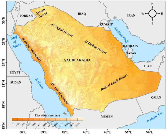
Figure 1.
Geographical location map of the study area.
3. Data and Methods
3.1. Data
To achieve the purpose of this research, data obtained from various sources were used, including simulated surface data, satellite products, and soil data. The details of the data used are presented in Table 1. The satellite products used in this study included Normalized Difference Vegetation Index (NDVI), land surface temperature (LST), AOD, and precipitation information. NDVI and LST data were obtained from MOD13C2 and MOD11C3 products of Moderate Resolution Imaging Spectroradiometer (MODIS) with a spatial resolution of 5000 m. To extract AOD information, the MCD19A2 product with a spatial resolution of 1000 m was used. These data are available at https://earthexplorer.usgs.gov/ website (10 April 2023). Rainfall information was extracted from TRMM satellite data with a spatial resolution of 25,000 m. These data are available at https://giovanni.gsfc.nasa.gov/giovanni/ website. Soil moisture data for 10 cm depth, wind speed at 10 m height, and air humidity were used from the Global Land Data Assimilation System (GLDAS). These data are simulated based on the combination of satellite and ground data based on numerical models. These data were derived from the https://giovanni.gsfc.nasa.gov/giovanni website (8 April 2023). Simulated data and satellite products were compiled for the period from 2000 to 2022. Additionally, soil information was derived from maps provided by the Food and Agriculture Organization (FAO). This information included soil texture and the composition of soil constituents, including the percentage of silt, sand, and clay, with a spatial resolution of 1000 m. The spatial resolution of various data and products was converted to 5000 m.

Table 1.
Details of the data used in the study.
3.2. Method
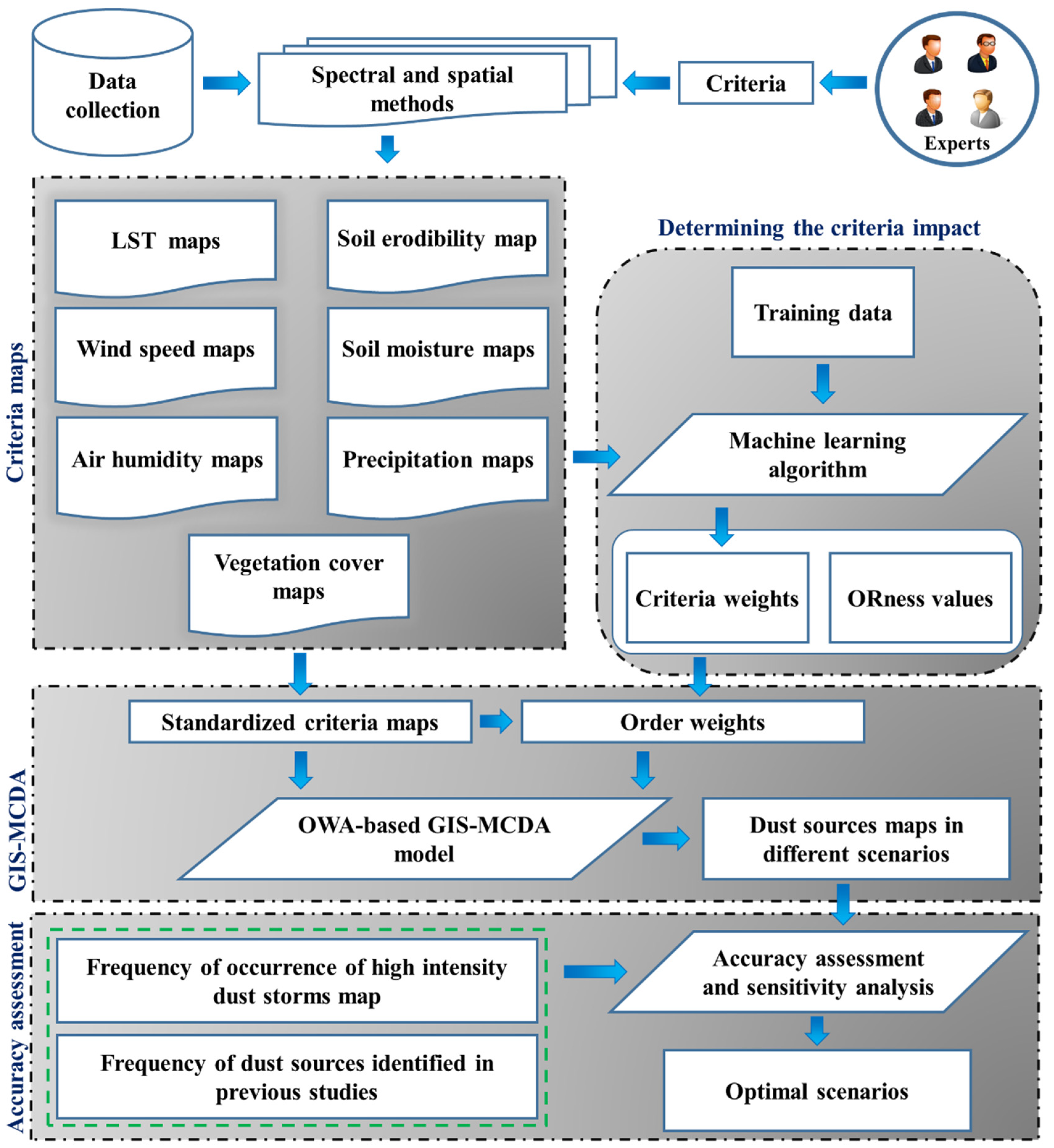
The proposed method in this study to identify SRDSFs includes four main steps (Figure 2). In the first step, according to the expert’s opinion and an in-depth examination of the relevant literature, criteria affecting the SRDSF identification process were identified and maps of various criteria were prepared. In the second step, the weight of effective criteria (degree of importance) in SRDSF identification were determined, and previous dust source maps of the study area were generated based on a machine learning algorithm. In the third step, the ordered weighted averaging (OWA) model was employed to generate dust source maps in different scenarios (each scenario indicates a degree of optimism or pessimism or risk in the decision). In the fourth step, the accuracy and spatial compatibility of SRDSFs identified in different scenarios were evaluated based on the frequency of dust sources obtained from the previous studies and the frequency of occurrence (FoO) of high AOD values.
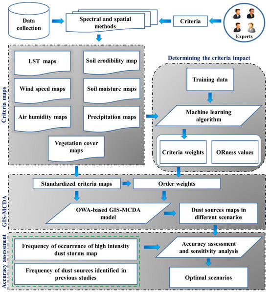
Figure 2.
The proposed method to identify SRDSFs in this study.
3.2.1. Effective Criteria
First, a map database of criteria affecting the identification of SRDSFs was prepared based on the opinion of experts and a review of past studies [30,37,41,48]. In this study, the opinions and expertise of 35 specialists with backgrounds in dust storms, dust-storm-prone regions, desertification, environmental studies, and natural resources were utilized. The selection criteria for these experts included having practical and research experience that is particularly relevant to the identification and mitigation of SRDSFs. These effective criteria included vegetation cover, soil moisture, soil erodibility, wind speed, precipitation, and absolute air humidity. The type of impact of these criteria on the creation of SRDSFs was presented.
Vegetation cover: This parameter acts as a natural mechanical barrier and causes a decrease in wind speed and generally decreases the power of wind erosion on the soil surface. In areas with poor vegetation, the risk of soil erosion and subsequent occurrence of dust is much higher than in areas with dense vegetation.
Soil moisture: Dry soils are much more erosive in front of the wind compared to wet soils, which is due to the reduction of adhesion between soil particles due to the reduction of soil moisture. With the increase of soil moisture, the threshold speed of wind erosion increases. Hence, dust storms are strongly associated with dry climates.
Soil erodibility: Soil erodibility is considered an effective factor in the formation of SRDSF. Soil particles with lower erodibility are more prone to wind erosion and can be carried more easily. On the other hand, soil erodibility is an important factor in determining the amount of moisture capacity and particle adhesion. In this study, the soil erodibility coefficient was calculated based on the soil texture information including the amount of clay, silt, and sand (Table 2) [70].

Table 2.
Soil erodibility coefficients for different soil texture.
Wind speed: Wind is one of the main factors in dust storms. The wind causes uprooting and movement of particles and also reduces the surface soil moisture. In general, with the availability of other environmental conditions, the wind speed exceeding a threshold is necessary to create a dust storm. Therefore, wind speed can be introduced as a limiting factor concerning the formation of the dust source. Obviously, as the wind speed increases, the probability of dust source formation in an area increases.
Precipitation: With the decrease in precipitation, the moisture content of soil and vegetation decreases. Following the reduction of surface soil moisture and vegetation, soil particles are more easily and quickly affected by wind erosion. As a result, the potential for SRDSF formation is greater for areas with less precipitation.
Air humidity: There is an inverse relationship between air humidity and dust occurrence. An increase in air humidity increases the amount of water in the surface soil layer and causes a decrease in the possibility of the formation of SRDSF, such that with the decrease in air humidity, dust will occur when the wind blows, even with low power, due to the dryness of the surface soil layers.
LST: As the surface temperature increases, the amount of evaporation from the surface increases. As a result, the dry soil particles are unstable due to the lack of adhesive force caused by the thin layer of water between the particles, and in this case, the wind is easily able to transport the soil particles.
In terms of the type of influence, the effective criteria can be divided into two groups. The first group of criteria includes wind speed and LST, which have a direct impact on the formation of dust centers. The second group of criteria includes vegetation, soil moisture, rainfall, LST, and absolute air humidity, which are involved in the formation of SRDSFs. Therefore, for the standardization of the criteria of the first and second groups, the minimum (Equation (1)) and the maximum (Equation (2)) methods were used, respectively.
where aij is the standardized value of the ith position for the jth criterion. Furthermore, Sij is the value of the ith position for the jth criterion, is the lowest value, and is the highest value of the jth criterion.
In addition to effective criteria, limiting layers were also used in the process of identifying SRDSFs. Based on experts’ opinions and review of previous studies in similar areas, two factors of vegetation cover (NDVI threshold less than 0.15) and wind speed (threshold less than 6 m/s) were selected as limiting layers [54,71,72].
3.2.2. Criteria Weight Calculation
In this study, the random forest algorithm was employed as a machine learning model. The random forest algorithm is an ensemble algorithm that utilizes decision trees for classification [73,74,75,76,77]. In the random forest algorithm, multiple decision trees are used. Essentially, a collection of decision trees collectively forms a forest, and this forest can make better decisions (compared to a single tree). In this study, 100 trees were considered. The random forest algorithm ultimately selects the class with the highest number of votes through voting and assigns it as the final class for classification tasks. The level of contribution of each variable in classification is calculated using the variables’ importance function, which is one of the outputs of the random forest algorithm [77,78]. Hence, to determine the degree of importance of effective criteria in the identification of SRDSFs for the study area, the variables’ importance function output was used. The input of the random forest algorithm includes the values of the effective criteria in the sample points specified as SRDSFs and nonsources. In this study, two reference data were used to select training samples as SRDSFs: (1) Areas designated as dust sources in past studies with high frequency. The high-frequency threshold was set at 8. This means that geographic locations that have been identified as centers in a minimum of 8 studies were selected as the training samples of SRDSFs. (2) Areas with a frequency greater than 350 days AOD > 0.7 in the period from 2000 to 2022. The minimum and maximum values of FoO of AOD > 0.70 for the study area ranged from 20 to 425 days. This means that in some geographic locations within the study area, AOD values exceeding 0.7 have occurred for up to 425 days from 2000 to 2022. When the FoO of AOD > 0.70 is higher in a geographic location, it indicates a higher probability of being an SRDSF in that geographic area. The obtained values for FoO of AOD > 0.70 were categorized into quartiles. The value of 350 was calculated as the lower limit of the fourth quartile, which in this study serves as the threshold for selecting the training samples of SRDSFs based on the FoO of AOD > 0.70 map.
3.2.3. SRDSF Mapping in Different Scenarios
One of the decision-making methods that can include the degree of risk taking and risk aversion of managers and planners in decision-making issues is the OWA method. Yager [79] developed the OWA operator to provide a method for combining criteria in multicriteria decision making based on the risk factor. In the past years, the OWA model was used in various spatial applications, such as determining suitable areas for the construction of solar and wind power plants, land suitability, physical expansion of cities, etc. [80,81,82,83,84,85,86].
The OWA model has high flexibility and capability in defining and using different combination operators because this operator is not defined by a parameter but by a weight vector. By choosing the appropriate weight vector, it is possible to model various types of relationships between the criteria that are to be combined. Therefore, different scenarios can be modeled based on this model.
The n-dimensional operator of OWA is a mapping from the Rn to R space, which is applied to aggregate the inputs of a system and has a weight vector in the form of W = [w1, w2, …, wn], so that each member of this vector is in the interval [0, 1] and is described using Equation (3):
where vj is the order weight, wj is the criterion weight, and Zij is the attribute value of the j index of the i pixel that has been standardized and hierarchically assigned. In this method, two types of weights are used, including order weight and criteria weights. Order weights are assigned based on the location of each pixel in criteria, but criteria weights show the relative importance of one criterion compared to another criterion and are the same for all pixels in a criterion. Therefore, in a criterion map, all pixels have the same criterion weight, but their order weight is different. The sequence Zi1 ≥ Zi2 ≥ Zi3 ≥ … ≥ Zin is generated by ordering the standard values of the criteria in the i-th location. The j-th criterion weight, wj, is reordered according to the ordered values of the criteria, Zij. The first-order weight v1 is assigned to the largest value of criteria in the i-th location, the second-order weight v2 is assigned to the second-largest value of the criteria in the same location, and vn is assigned to the smallest criterion value in the that location. A certain amount of Zij does not have a specific weight vj, but the weight belongs to the ordered position of Zij.
The ORness parameter in the OWA model indicates the degree of risk taking or risk aversion of the decision maker. The degree of ORness is calculated based on Equation (4).
The higher the value of ORness, the higher the degree of optimism or risk taking of the decision maker, and the lower the value of ORness, the higher the degree of pessimism or risk aversion of the decision maker (Figure 3). Usually, an ORness value less than 0.5 indicates a risk-averse decision maker, equal to 0.5 is a neutral decision maker, and more than 0.5 indicates a risk-taking decision maker [80,81,82].
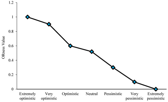
Figure 3.
The relation between decision-making conditions of mental and ORness values [83].
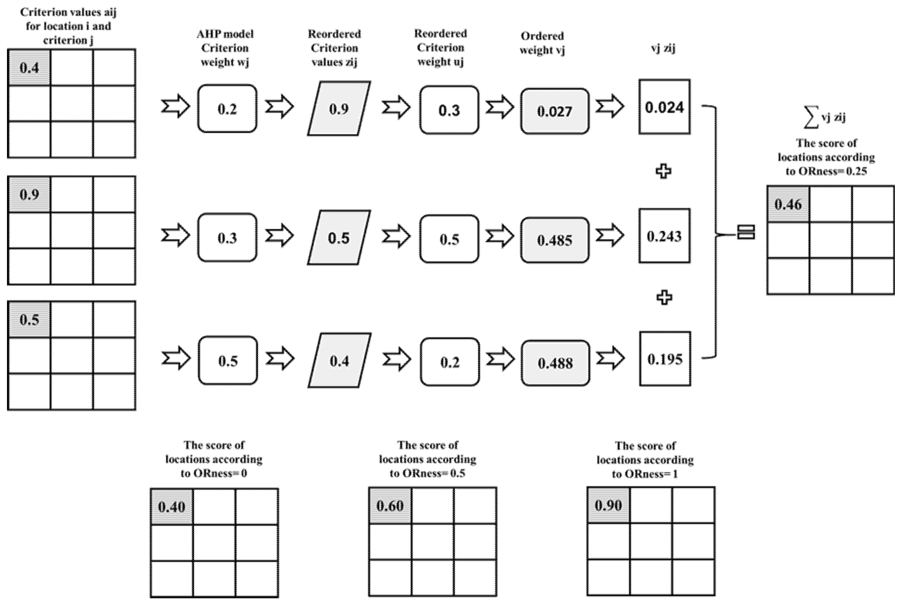
An example of OWA method calculations in different scenarios (different ORness) is described in Figure 4.
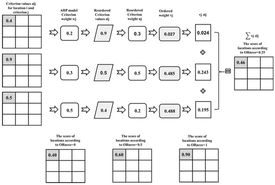
Figure 4.
Schematic computation of the OWA for the ith location with different ORnesses = 0, 0.25, 0.5, and 1 [27,86].
In this study, the proposed method was used to prepare potential maps of SRDSFs in 5 different scenarios, including very optimistic, optimistic, neutral, pessimistic, and very pessimistic. Potential maps of SRDSFs were classified into dust source and nondust source classes by defining the appropriate threshold limit. The natural breaks clustering method was used to determine the appropriate threshold. The method optimizes for total intraclass variance, making the classes as homogeneous as possible.
3.2.4. Accuracy Assessment and Sensitivity Analysis
The extracted SRDSF map should be evaluated to use it more correctly and efficiently. One of the widely used methods in evaluating the accuracy of classification results is the error matrix, which can be used to extract a series of descriptive and analytical statistics. In this study, based on the confusion matrix, the four metrics of omission error, commission error, overall accuracy, and prediction rate were calculated.
Commission error shows the ratio of the area of regions wrongly classified in the class of SRDSF to the actual area of nondust source regions in the study area. In other words, the larger the area of the regions that are wrongly classified in the class of SRDSFs, the higher the commission error value. These regions were not SRDSFs in reality, but they were classified as SRDSFs in the output of the model. Omission error shows the ratio of the area of the regions that were dust sources but not classified in the dust source class to the actual area of the dust sources in the study area. In other words, the larger the area of the real SRDSFs that are not detected, the higher the omission error. The overall accuracy shows the ratio of the total area of correctly classified areas in the SRDSF and nondust source classes to the area of the studied area. To calculate the prediction rate, the value of “producer’s accuracy for dust source class” is divided by the value of “the ratio of the area of the regions identified as SRDSFs to the area of the study area”. The higher the prediction rate for a model, the higher the efficiency of the model.
In this study, to compare and evaluate the dust source maps obtained from different scenarios, the FoO of AOD > 0.7 maps and the dust sources identification map in previous studies were used as the basic and real maps. In this study:
- The accuracy of identified SRDSFs in different scenarios was evaluated based on different thresholds of FoO of AOD > 0.7.
- The accuracy of identified SRDSFs in different scenarios was evaluated based on the frequency of dust source identification in previous studies [30,56,63,64,65,66].
After evaluating the accuracy of different scenarios, the optimal scenario was determined to prepare a map of existing SRDSFs in the study area. Then, the sensitivity of the areas designated as SRDSFs based on the optimal scenario was evaluated concerning the effective criteria. One of the most important factors in most sensitivity analysis methods is to investigate the effect of changing the weight of criteria on the output of MCDA models. In this study, the one-at-a-time method was used [86]. In this method, sensitivity analysis was performed with systematic changes in the weight of the criteria and checking its effect on the area change of the regions identified as SRDSFs. In the first step, the weight of each criterion was changed between 0 and 1 with a step size of 0.1. In the second step, after each change in the weight of a criterion, the weight of other criteria was changed to compensate for the change in weight according to their suitability because the sum of the weights of the criteria must be 1 in each step. In the third step, after the weights of the criteria were updated in each step, dust source maps were produced for the optimal scenario, and the area of the identified SRDSF was calculated. If the change in the weight of a criterion from 0 to 1 slope significantly changed the area of the identified SRDSF, it indicated the high sensitivity of the model output to this criterion.
4. Results
4.1. Effective Criteria Weights
The weight of each criterion indicates the importance degree and its impact on the preparation of the SRDSF map. The weights obtained for each criterion using the machine learning method are shown in Figure 5. The weights of the criteria of vegetation cover, soil moisture, soil erodibility, wind speed, precipitation, LST, and air humidity were 0.15, 0.17, 0.22, 0.21, 0.05, 0.13, and 0.07, respectively. Soil erodibility and precipitation criteria had the highest and lowest impact in identifying dust sources, respectively. After soil erodibility, the wind speed criterion had the highest importance degree in identifying SRDSFs. This result shows that for areas with high soil erodibility and wind speed, the possibility of SRDSFs is high.
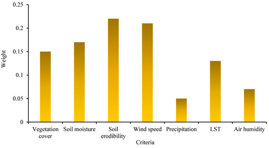
Figure 5.
Calculated weights for effective criteria in identifying SRDSFs based on a machine learning model.
4.2. Identified SRDSFs in Different Scenarios
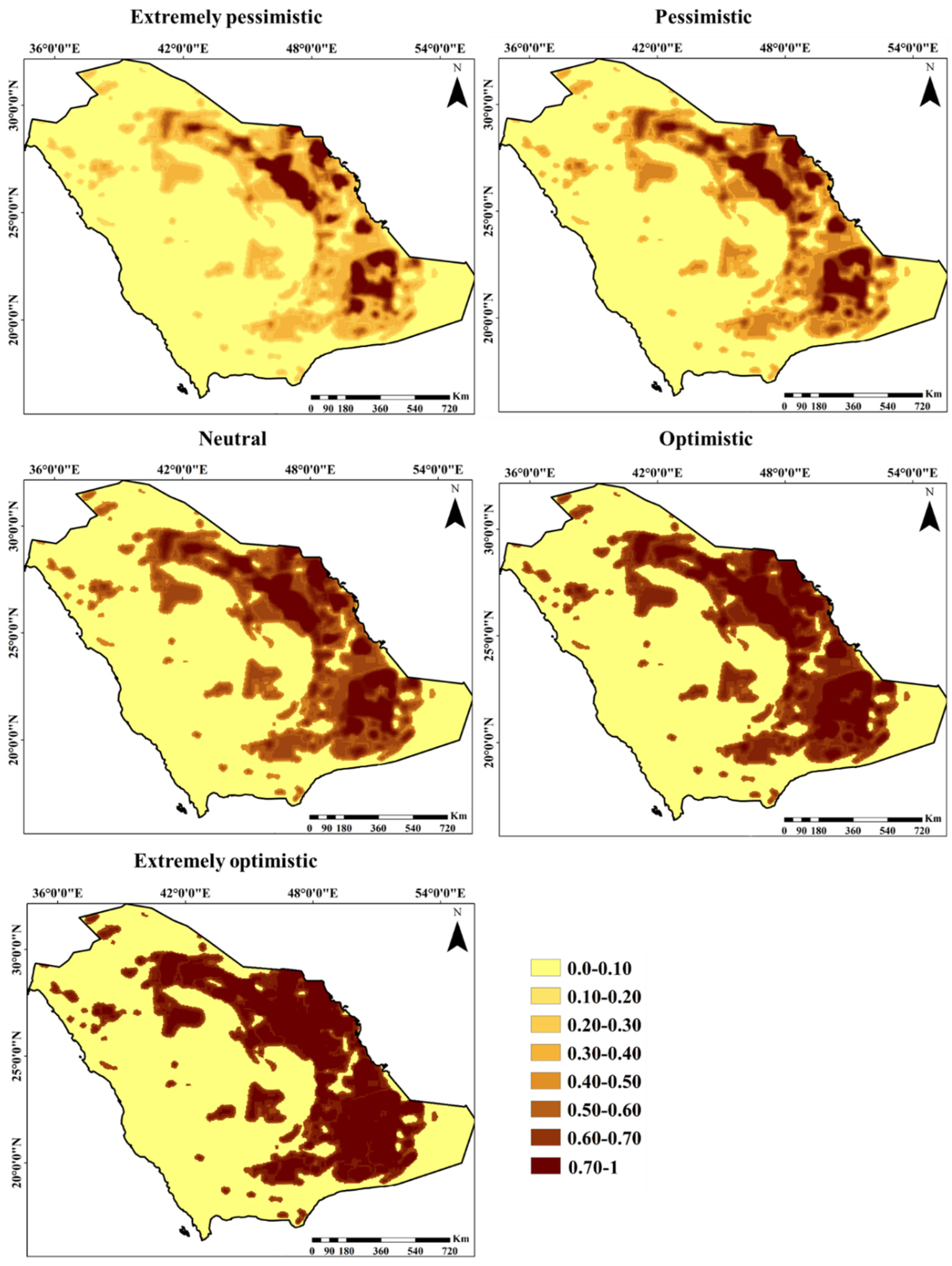
The potential maps of SRDSFs in five scenarios from very pessimistic to very optimistic are shown in Figure 6. The values of these maps vary between 0 and 1. The value 0 indicates the regions with the lowest potential for creating SRDSFs and the value 1 indicates the regions with the highest potential for creating SRDSFs. The evaluation of the potential maps shows that with the increase in the degree of optimism, the area of the regions with high potential for creating SRDSFs increases, and, on the other hand, the risk in decision making also increases. The average values of the SRDSF potential maps in very pessimistic, pessimistic, neutral, optimistic, and very optimistic scenarios are 0.22, 0.26, 0.35, 0.41, and 0.48, respectively. By increasing the degree of optimism (risk degree) in the model, the average potential of SRDSFs in the study area increases. Regions with very high potential (0.7–1) are deliberately located in the eastern and southeastern regions. Also, most of the western, central, and northwestern regions have very low potential (0–0.1).

Figure 6.
Potential maps of SRDSFs produced in different scenarios.
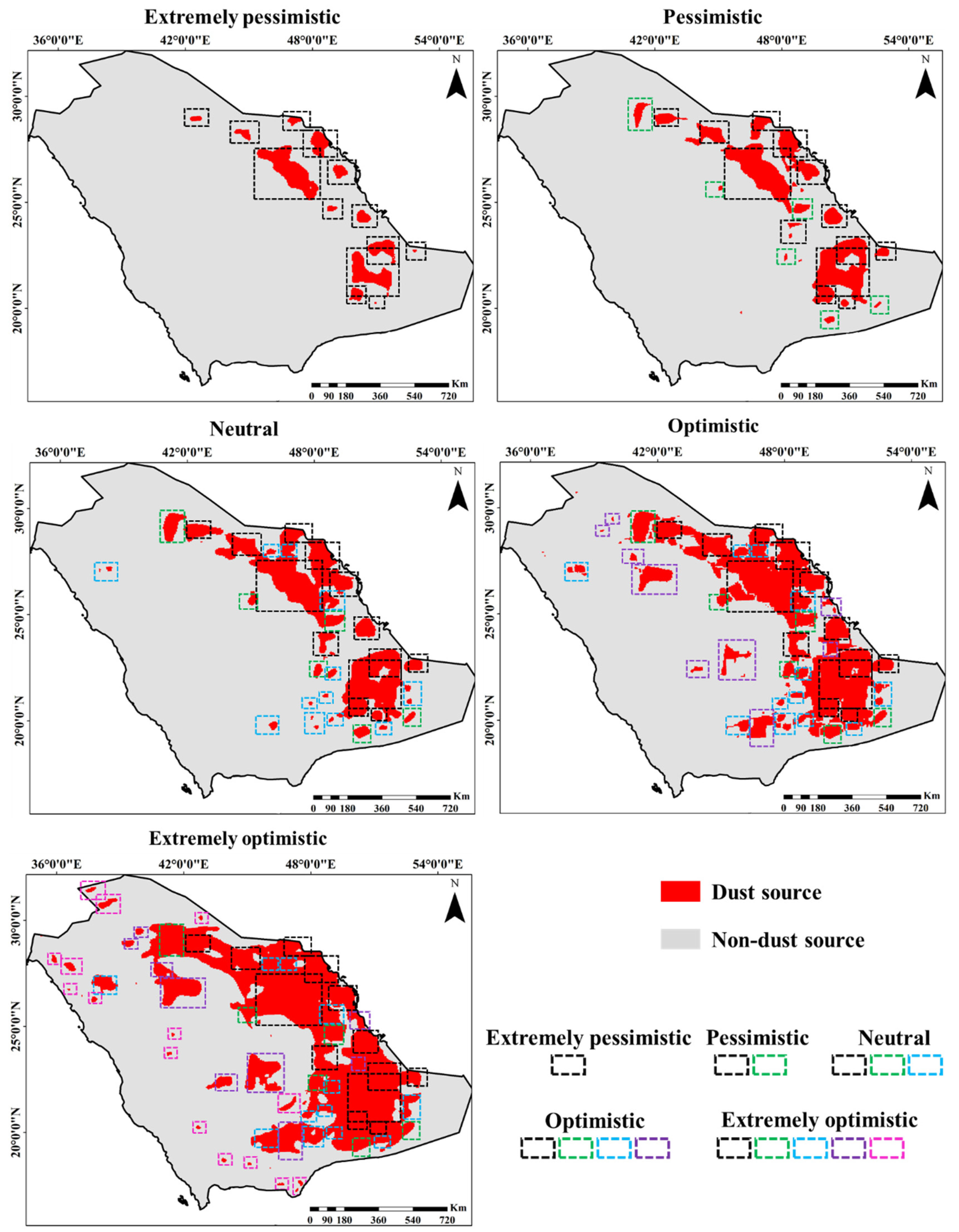
By defining the threshold limit on the potential maps, the study area was classified into two classes of SRDSF (areas with values above 0.6), and non-SRDSF (areas with values less than 0.6) and SRDSF were identified (Figure 7). The areas identified as SRDSFs in very pessimistic, pessimistic, neutral, optimistic, and very optimistic scenarios were 85,950, 168,275, 255,225, 410,000, and 596,500 km2, respectively. Based on the analysis of the spatial patterns of the regions identified as sources, 13, 19, 31, 40, and 55 sources were identified for each of these scenarios. The area and the number of SRDSFs detected from the very pessimistic scenario to the very optimistic scenario increased by 594 and 323%, respectively. The results show that by increasing the degree of risk in decision making (increasing the degree of optimism) in addition to increasing the area of existing SRDSFs, new SRDSFs were also identified.
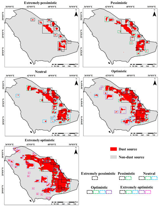
Figure 7.
Maps of identified SRDSFs in different scenarios. Color-coded boxes represent the identified SRDSFs in different scenarios. For example, boxes with a black border indicate areas that were identified as SRDSFs in a very pessimistic scenario. In a very optimistic scenario, all boxes with different colors were identified as SRDSFs.
4.3. Accuracy Assessment of Identified SRDSFs in Different Scenarios
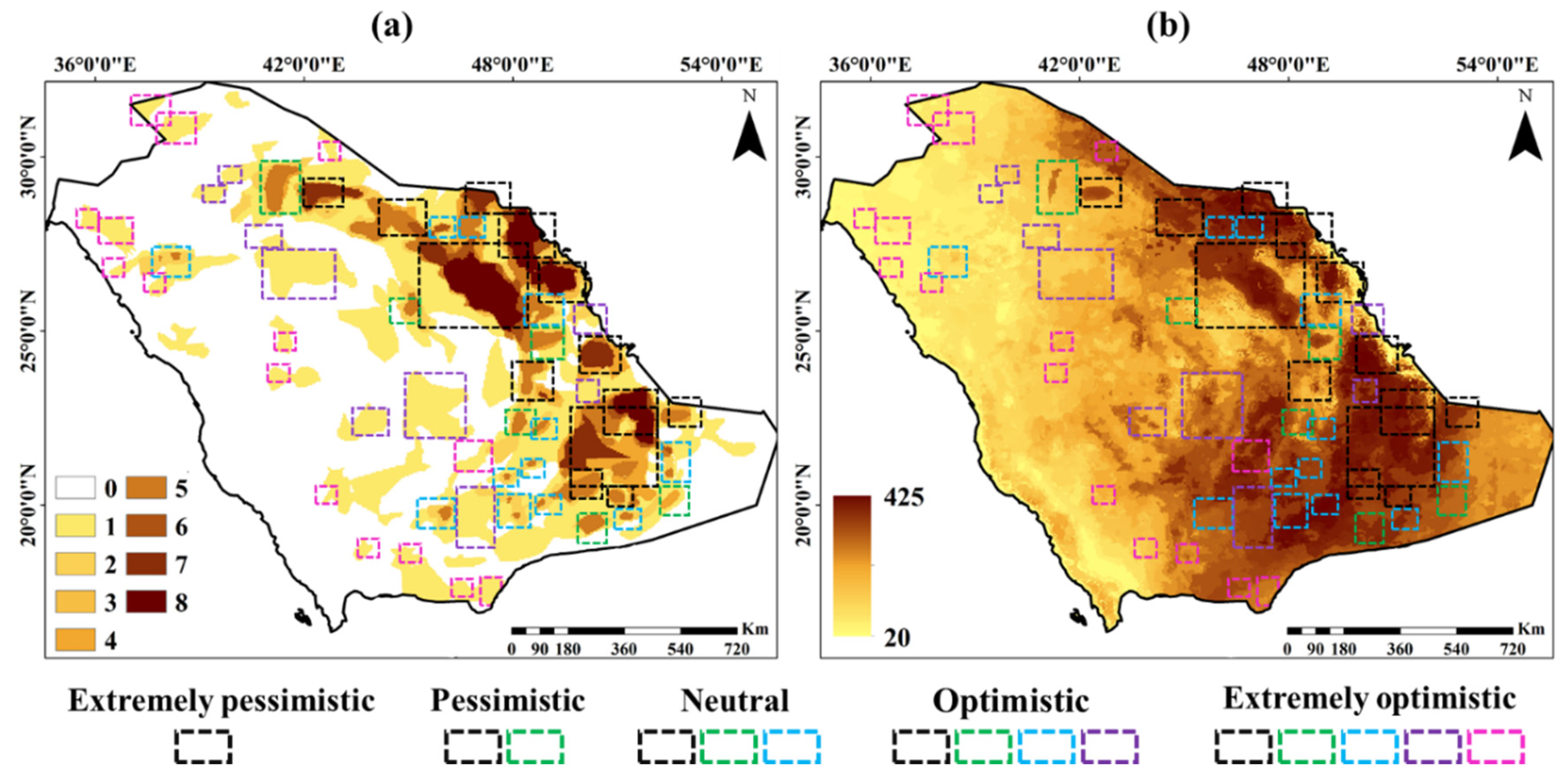
The spatial matching of SRDSFs extracted in different scenarios in this study with (1) frequency of dust sources obtained from the previous studies and (2) FoO of AOD > 0.7 from 2000 to 2021 is shown in Figure 8. The average frequency of dust sources obtained from the previous studies in the geographical location of SRDSFs identified in very pessimistic, pessimistic, neutral, optimistic, and very optimistic scenarios were 7, 6, 5, 4, and 3, respectively. FoO of AOD > 0.7 varied between 20 and 425 days. Spatially, most of the SRDSFs detected in the very pessimistic scenario correspond to the high-frequency values of sources obtained from previous studies and FoO of AOD > 0.7. But many of the SRDSFs identified in the optimistic and very optimistic scenarios were only identified as dust sources in previous studies. Also, the value of FoO of AOD > 0.7 was low in a large number of SRDSFs identified in these scenarios. In other words, choosing these areas as SRDSFs has a high risk. The correlation coefficients between the potential values of SRDSFs estimated based on very pessimistic, pessimistic, neutral, optimistic, and very optimistic scenarios and FoO of AOD > 0.7 are 0.60, 0.67, 0.72, 0.78, and 0.86, respectively.
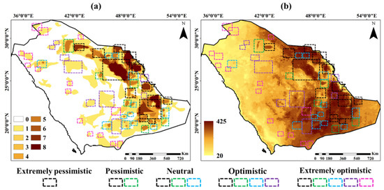
Figure 8.
Maps of (a) frequency of dust sources obtained from the previous studies and (b) FoO of AOD > 0.70 in unit days from 2000 to 2021, and geographical location of identified SRDSFs in different scenarios. Color-coded boxes represent the identified SRDSFs in different scenarios. For example, boxes with a black border indicate areas that were identified as SRDSFs in a very pessimistic scenario. In a very optimistic scenario, all boxes with different colors were identified as SRDSFs.
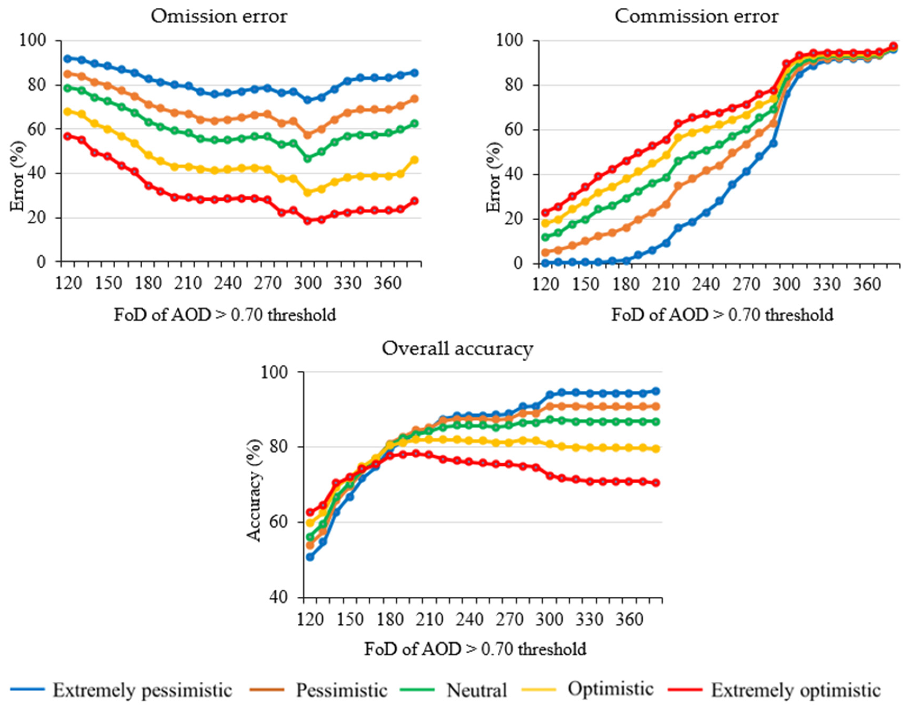
By changing the threshold limit of FoO of AOD > 0.7 (variable between 120 and 380 with a step size of 10), different base maps were produced, and then the accuracy of SRDSFs identified in different scenarios was evaluated based on these base maps (Figure 9). The lowest omission error for all different thresholds of FoO of AOD > 0.7 was for the very optimistic scenario. Therefore, in this scenario, a high percentage of SRDSFs based on FoO of AOD > 0.7 was detected. Omission error for all scenarios has a decreasing trend for thresholds of 120 to 310 days, while it has an increasing trend for thresholds of 310 to 380 days. But in terms of commission error, the most pessimistic scenario has the highest accuracy, and the commission error increases as the degree of optimism increases. In other words, with the increase in the degree of optimism, the areas classified in the class of SRDSFs will increase incorrectly. By increasing the threshold value, the amount of SRDSFs based on FoO of AOD > 0.7 decreases; hence, by increasing the threshold value, the commission error increases in all scenarios. In this regard, for thresholds higher than 300 days, the commission error in all scenarios increases significantly and reaches above 80%. The results of the overall accuracy metric show that for thresholds less than 180 days, the very optimistic scenario has the highest accuracy. On the other hand, for the threshold limit of more than 180 days, the very pessimistic scenario has the highest accuracy.
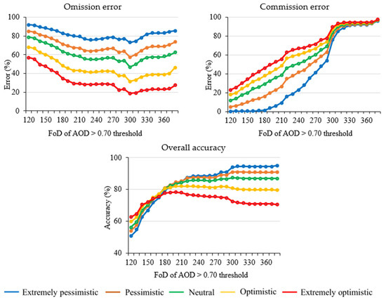
Figure 9.
The results of evaluating the accuracy of identified SRDSFs in different scenarios based on different thresholds of FoO of AOD > 0.7.
The average values of the evaluation metrics of different scenarios based on different thresholds of FoO of AOD > 0.7 are shown in Table 3. The results showed that the very pessimistic and very optimistic scenarios had the highest omission and commission errors of dust source identification in the study area, respectively. The overall accuracy of these scenarios in identifying SRDSFs in the study area was 84.1, 83.3, 81.6, 78.2, and 73.2 %, respectively. Also, the very pessimistic scenario had the highest prediction rate value, which indicates that the very pessimistic scenario has a high ability to identify SRDSFs with high confidence.

Table 3.
The average values of evaluating metrics for the accuracy of identified SRDSFs in different scenarios based on AOD.
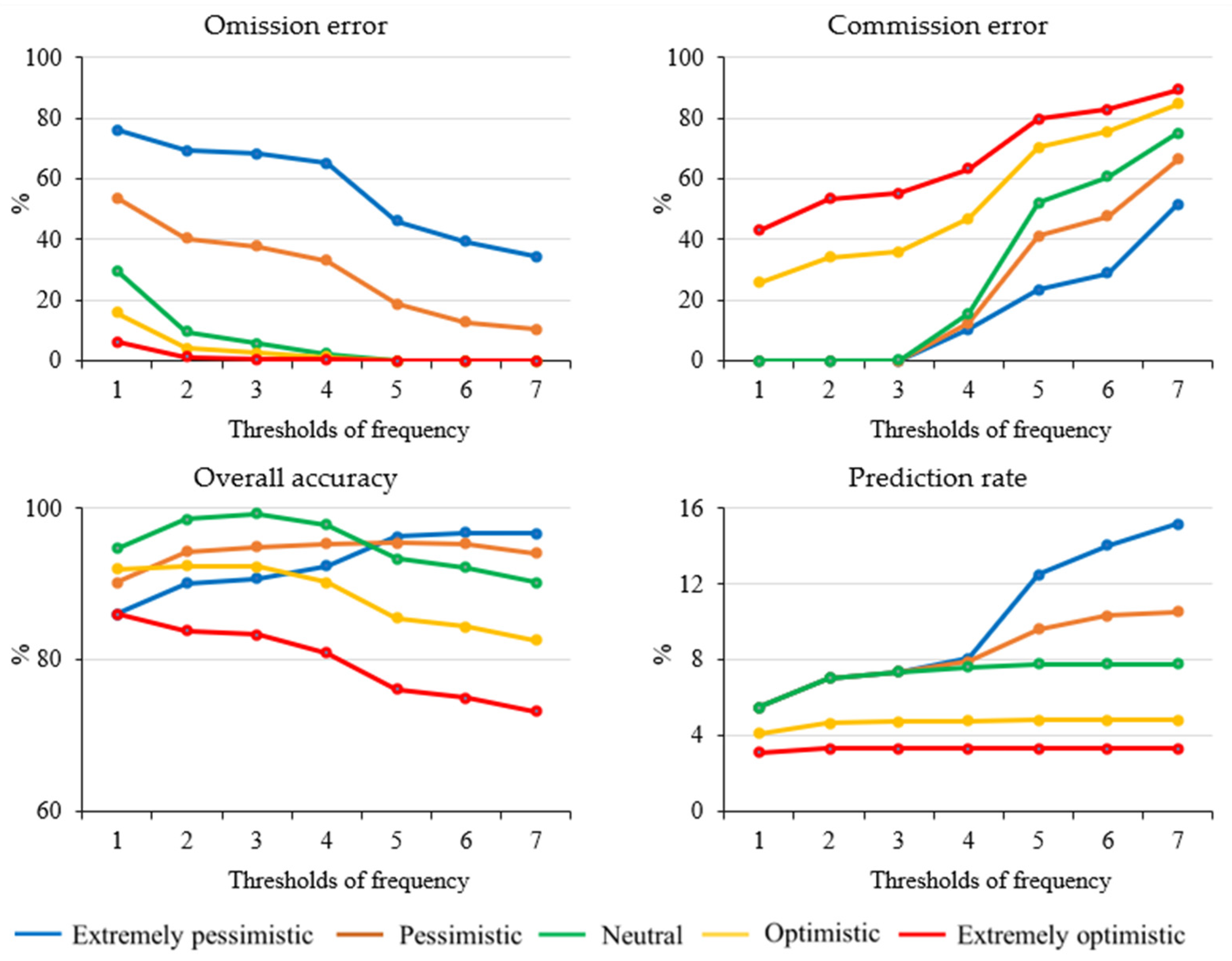
By changing the frequency of dust sources obtained from the previous studies (variable between one and eight with a step size of one), different base maps were produced and the accuracy of SRDSFs identified in different scenarios was evaluated with these base maps (Figure 10). By increasing the threshold limit, the omission and commission errors in all scenarios decreased and increased, respectively. In terms of omission and commission errors, the very optimistic and very pessimistic scenarios had the best performance in identifying SRDSFs, respectively. For the limit of thresholds greater than four, the omission error of neutral, optimistic, and very optimistic scenarios was zero. For the limit of thresholds less than four, the commission error of neutral, pessimistic, and very pessimistic scenarios was zero. The overall accuracy of identifying SRDSFs for the optimistic scenario was lower than other scenarios at all thresholds. In general, with the increase of the threshold value, the overall accuracy of all scenarios decreased, except for the very pessimistic scenario. For the limit of thresholds less than five, the overall accuracy of the neutral scenario was higher than other scenarios, but for the limit of thresholds greater than five, the efficiency of the very pessimistic scenario was higher than other scenarios. Evaluating the results of the prediction rate metric shows that the efficiency of the pessimistic scenario was higher than other scenarios at all thresholds.
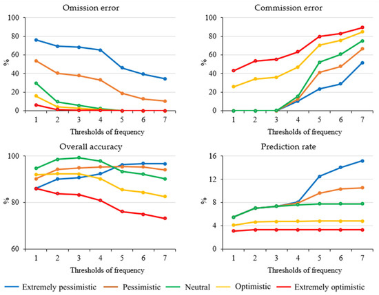
Figure 10.
The results of evaluating the accuracy of identified SRDSFs in different scenarios based on dust sources obtained from the previous studies in different thresholds on frequency.
The average values of the evaluation metrics of different scenarios based on the frequency of dust sources obtained from the previous studies are shown in Table 4. The results showed that very optimistic and very pessimistic scenarios had the highest omission and commission errors of SRDSF identification in the study area, respectively. The average overall accuracy of these scenarios in identifying SRDSFs in the study area was 92.7, 94.2, 95.1, 88.4, and 79.7%, respectively. The very pessimistic scenario had the highest prediction rate, which indicates that the very pessimistic scenario has a high ability to identify SRDSFs with high confidence.

Table 4.
The average values of evaluating metrics for the accuracy of identified SRDSFs in different scenarios based on dust sources obtained from the previous studies.
The spatial accuracy assessment of SRDSFs identified in different scenarios with the dust sources identified in previous studies is shown in Figure 11. The results show that 85,950, 168,275, 255,200, 305,800, and 340,250 km2 of the dust sources identified in the previous studies were correctly identified using very pessimistic, pessimistic, neutral, optimistic, and very optimistic scenarios, respectively. In the very pessimistic scenario, compared to other scenarios, a small area of dust sources identified in previous studies was identified. In very pessimistic, pessimistic, neutral, optimistic, and very optimistic scenarios, respectively, 276,725, 194,400, 107,475, 56,875, and 22,425 km2 of dust sources identified in previous studies were not identified. In the very pessimistic scenario to the neutral scenario, the identified SRDSFs exactly matched the sources identified in previous studies; therefore, in these scenarios, no regions were wrongly identified as dust sources. But in the optimistic and very optimistic scenarios, the wrongly identified sources increased. In these scenarios, 104,150 and 256,175 km2 were wrongly identified as SRDSFs, respectively. In general, with the increase in the degree of optimism, the number of wrongly identified sources increases.
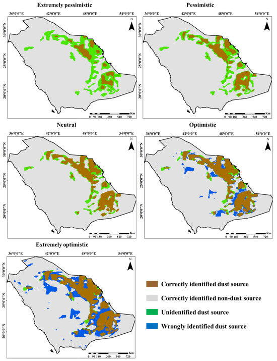
Figure 11.
Maps for evaluating the spatial accuracy of identified SRDSFs in different scenarios based on dust sources obtained from the previous studies with frequency > 2.
4.4. Sensitivity Analysis
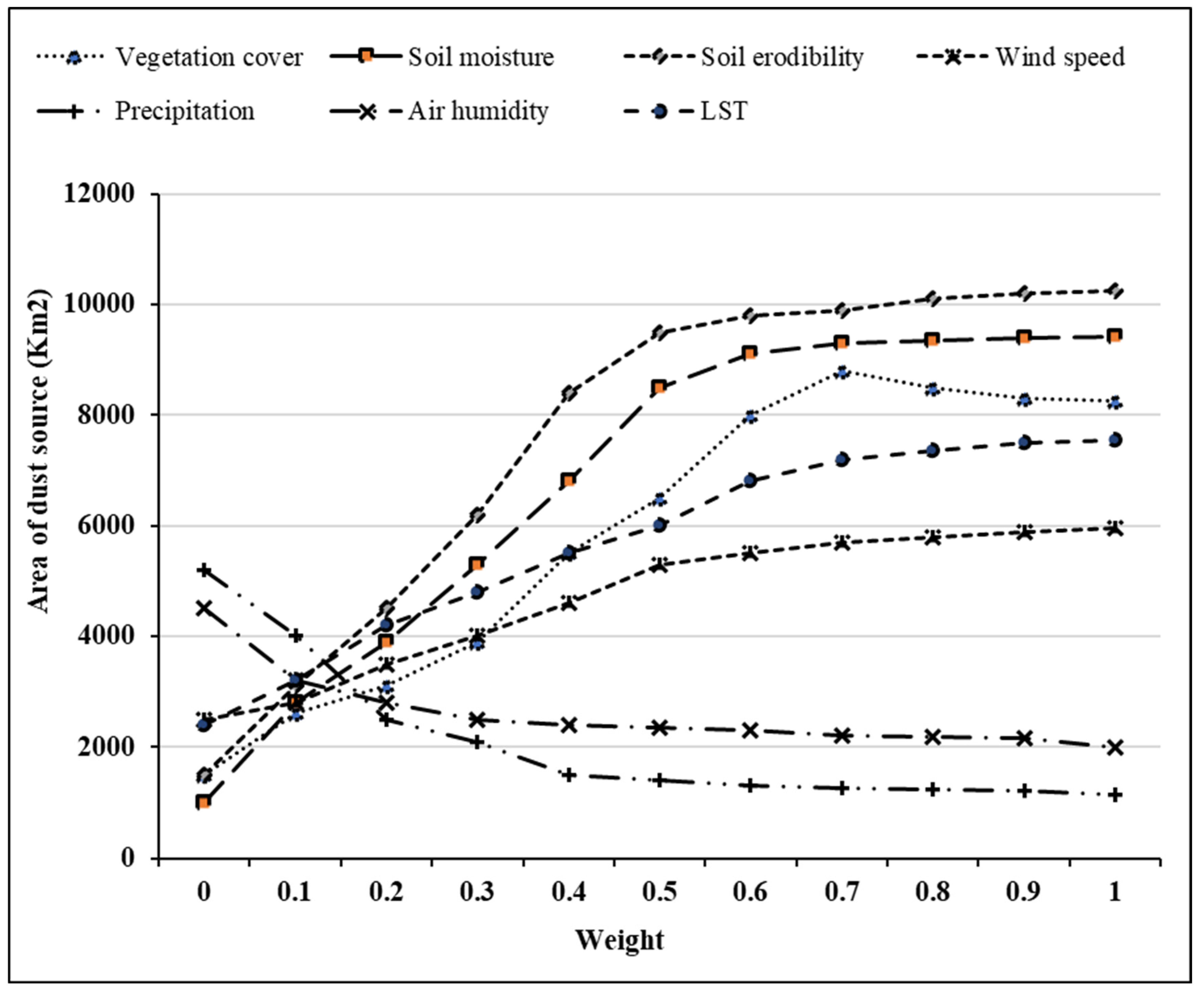
The results of the sensitivity analysis of the criteria weight change on the area of the identified SRDSFs are shown in Figure 12. Determining SRDSFs for the study area is most sensitive to the soil erodibility, soil moisture, and vegetation cover criteria, and changing the weights of each of these criteria has a great impact on the area of identified SRDSFs. In this regard, it is very important to accurately determine the weights of these criteria. Changing the weights of precipitation and humidity criteria between 0 and 0.4 causes a large change in the area of identified SRDSFs, but increasing the weights of these criteria from 0.4 to 1 will not have much effect on the area of identified SRDSFs. By increasing the weights of the air humidity and precipitation criteria, the area of the identified SRDSFs decreases. On the other hand, increasing the weights of other criteria increases the area of identified SRDSFs.
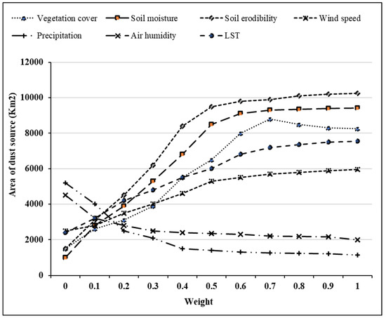
Figure 12.
Sensitivity analysis of the identified SRDSFs area to the change in the criteria weights.
5. Discussions
The accuracy of identifying SRDSFs depends on environmental factors and the model used. In this study, a set of environmental factors were used as effective criteria and several limiting factors to separate areas with the potential for the formation of SRDSFs from nonsusceptible areas. In this study, LST, soil moisture, vegetation cover, precipitation, wind speed, air humidity, and soil erodibility were used as effective criteria. Also, the map of limiting factors was prepared using wind speed and vegetation factors. The results showed that the criteria of wind speed and precipitation have the highest degree of importance in identifying SRDSFs. Boloorani, et al. [41] and Alsubhi, et al. [30] also confirmed this result. In several studies in similar regions, these effective criteria and limiting factors were used to identify SRDSFs. Boloorani, et al. [41] showed that the wind speed and LST factors have a direct effect, and the factors of vegetation cover, soil moisture, precipitation, and air humidity have an inverse effect, on the formation of SRDSFs. This result was also confirmed in other studies [87,88,89,90]. Fécan, et al. [91] showed that with increasing soil moisture, the adhesion of soil particles increases and the possibility of dust source formation decreases. In other studies, it was also shown that greater adhesion of soil particles reduces wind erosion [92,93]. Boloorani, et al. [37] demonstrated that, assuming other environmental conditions remain constant, regions with lower vegetation coverage and lower humidity compared to other areas have a higher potential for the formation of SRDSFs. Mayaud, et al. [87] showed that the weak surface vegetation cover causes a higher effect of wind on soil erosion. Hence, the higher the amount and density of vegetation cover in a region, the lower the probability of dust source formation. Wang, et al. [94] and Zhou, et al. [95] showed that the wind speed factor has a significant effect on the formation of SRDSFs through two aspects, including (1) creating the necessary force for wind erosion and (2) increasing transpiration and reducing soil moisture [94]. In several studies, it was shown that with the increase of precipitation in a geographical location, the probability of the formation of SRDSFs decreases [96,97]. Middleton [97] found that precipitation has a significant impact on the formation of SRDSFs in a given area, with an increase in precipitation leading to a reduction in the probability of SRDSF formation. Ravi, et al. [98] showed that increasing air humidity reduces the probability of SRDSFs forming in a region. The results of previous studies showed that the increase in LST causes a decrease in surface soil moisture and an increase in the probability of the formation of SRDSFs [96,99,100,101]. Boloorani, et al. [41] showed that with the increase of the soil erodibility coefficient, the probability of the formation of SRDSFs increases.
In this study, a risk-based decision-making method was developed to identify SRDSFs. This method is suitable and usable for a wide range of managers and decision makers. This method can produce maps of SRDSFs based on different mental attitudes, including very optimistic, optimistic, neutral, pessimistic, and very pessimistic. The OWA operator is used to implement this proposed method. In previous studies, OWA has been used as an operator in evaluating and producing suitable maps based on mental scenarios in various applications such as land use suitability, potential evaluation for earthquake and flood vulnerability, determining suitable areas for the construction of solar power plants, and urban growth. The results of these studies show the high flexibility of this operator. The models used in previous studies to identify SRDSFs can be meteorological- and statistical-based models, remote-sensing-based models, numerical-based models, and hybrid-based models. Each of these methods has advantages and disadvantages. In hybrid models used to identify SRDSF, effective environmental factors are prepared from different data sources [41,58,59,60,61,62,63]. The proposed model in this study is classified into a group of hybrid models. The proposed model does not limit the use of data obtained from different data sources. In this study, to implement the proposed model, remote sensing datasets, climatic data, simulations based on numerical models, and ground data were used simultaneously. To evaluate the results of different scenarios, two sources of information, the frequency of high AOD values and the geographical location of dust sources identified in previous studies, were used. These two methods were used in previous studies to evaluate the results of different models [30,41]. The frequency maps of high AOD values are more consistent with the results of the very pessimistic scenario, and the maps of dust sources identified in previous studies with the neutral scenario. However, the results of each of the implemented scenarios can be suitable for a certain group of managers and decision makers, depending on their mental attitudes and financial and time conditions.
In the results of this study, several factors can have an impact: (1) the population of selected effective criteria, (2) the accuracy of the sources used to prepare the criteria map, (3) the precision of the assigned weights to the effective criteria, and (4) the performance of the model used to combine the values of the effective criteria and their weights. In this study, expert opinions and previous studies were utilized to select effective criteria for forming SRDSFs. Expert opinions may be subject to uncertainty and disagreements among different experts [85]. The use of large-group decision making (LGDM) can reduce the uncertainty in the selection of effective criteria [102]. Additionally, effective criteria can vary for different geographical locations and time conditions, so reviewing past studies for their selection cannot be free of uncertainty. However, combining expert opinions and reviewing previous studies can significantly reduce uncertainty in the selection of effective criteria. For preparing the map of effective criteria in this study, simulated surface data, satellite products, and soil data were employed, each of which has its own errors and uncertainties. Consequently, the results of this study may also be accompanied by uncertainty stemming from the sources used to prepare the map of effective criteria. The weighting of criteria can significantly impact the uncertainty in the production of the SRDSF map. Figure 12 illustrates that changing the weight of each of the effective criteria results in a change in the identified SRDSF area. The sensitivity of the identified SRDSF area to changes in the weight of some criteria, such as precipitation and humidity, is higher than other criteria. Therefore, uncertainty in the weight of each of the effective criteria leads to uncertainty in the final identification of SRDSFs. Uncertainty arising from the performance of the model used to combine the values of effective criteria and their weights contributes to the uncertainty in identifying SRDSFs. In this study, the OWA model was employed to reduce this uncertainty, which is more flexible than other MCDA models [80,83,86]. The OWA model can map SRDSFs in different scenarios. Nevertheless, fuzzy-concept-based models and artificial intelligence-based algorithms also help reduce uncertainty and can be a focus of future studies.
6. Conclusions
Dust is one of the atmospheric phenomena and natural disasters that bring many environmental, economic, health, etc., consequences. Identification of SRDSFs not only greatly contributes to dust forecasting, early warning, and environmental impact assessment, but also has a profound and lasting impact on global climate change and human life. This study aimed to propose a risk-based method to identify SRDSF. For this purpose, the information of seven effective criteria, including vegetation cover, soil moisture, soil erodibility, wind speed, precipitation, and air humidity, was used. The OWA method was used to consider risk in the decision-making process. Wind speed and precipitation criteria had the highest and lowest degree of importance in identifying SRDSF, respectively. The proposed method had high flexibility in producing a wide range of dust source maps in the form of very pessimistic to very optimistic scenarios. As the degree of optimism increased, the decision risk increased. In the pessimistic scenario, the areas selected as SRDSFs were associated with a high percentage of confidence. But in the optimistic scenario, the confidence percentage of the extracted sources was low. The results of accuracy evaluation based on different sources showed that each of the scenarios can be effective in different conditions. The sources identified in the previous studies had a higher agreement with the results of the neutral scenario. The results showed that the very pessimistic and very optimistic scenarios had the highest error of omission and commission errors in identifying SRDSFs in the study area, respectively. The results of the sensitivity analysis of the weight of the criteria showed that the change in the weight of the criteria of vegetation cover, soil moisture, and soil erodibility is the most sensitive in the area of SRDSFs. In case of limited financial resources and the time required to manage SRDSFs, the results of very pessimistic and pessimistic scenarios can be more efficient. But in the absence of financial and time constraints, the results of very optimistic and optimistic scenarios can be used by managers and planners. The proposed method in this study can be used to determine SRDSFs in different scenarios in different regions of the world. This method is very practical and useful for managers and planners to reduce the adverse effects of the dust phenomenon.
Author Contributions
Y.A. and S.Q. conceived and designed the research of the first draft and wrote the first draft; Y.A. and S.Q. redesigned the research; S.Q., Y.A. and M.H.S. revised and edited the paper. All authors have read and agreed to the published version of the manuscript.
Funding
This research work was funded by Institutional Fund Projects under grant no. (IFPDP-241-22).
Data Availability Statement
The data used to support the findings of this study are available from the corresponding author upon reasonable request.
Acknowledgments
Therefore, the authors gratefully acknowledge technical and financial support from Ministry of Education, Deanship of Scientific Research (DSR), and King Abdulaziz University (KAU), Jeddah, Saudi Arabia.
Conflicts of Interest
The authors declare no conflict of interest.
References
- Adger, W.N.; Huq, S.; Brown, K.; Conway, D.; Hulme, M. Adaptation to climate change in the developing world. Prog. Dev. Stud. 2003, 3, 179–195. [Google Scholar] [CrossRef]
- Firozjaei, M.K.; Sedighi, A.; Mijani, N.; Kazemi, Y.; Amiraslani, F. Seasonal and daily effects of the sea on the surface urban heat island intensity: A case study of cities in the Caspian Sea Plain. Urban Clim. 2023, 51, 101603. [Google Scholar] [CrossRef]
- Firozjaei, M.K.; Fathololoumi, S.; Kiavarz, M.; Biswas, A.; Homaee, M.; Alavipanah, S.K. Land Surface Ecological Status Composition Index (LSESCI): A novel remote sensing-based technique for modeling land surface ecological status. Ecol. Indic. 2021, 123, 107375. [Google Scholar] [CrossRef]
- Firozjaei, M.K.; Weng, Q.; Zhao, C.; Kiavarz, M.; Lu, L.; Alavipanah, S.K. Surface anthropogenic heat islands in six megacities: An assessment based on a triple-source surface energy balance model. Remote Sens. Environ. 2020, 242, 111751. [Google Scholar] [CrossRef]
- Yang, J.; Zhou, M.; Ren, Z.; Li, M.; Wang, B.; Liu, D.L.; Ou, C.-Q.; Yin, P.; Sun, J.; Tong, S. Projecting heat-related excess mortality under climate change scenarios in China. Nat. Commun. 2021, 12, 1039. [Google Scholar] [CrossRef]
- Vicedo-Cabrera, A.M.; Scovronick, N.; Sera, F.; Royé, D.; Schneider, R.; Tobias, A.; Astrom, C.; Guo, Y.; Honda, Y.; Hondula, D. The burden of heat-related mortality attributable to recent human-induced climate change. Nat. Clim. Chang. 2021, 11, 492–500. [Google Scholar] [CrossRef]
- Lababpour, A. The response of dust emission sources to climate change: Current and future simulation for southwest of Iran. Sci. Total Environ. 2020, 714, 136821. [Google Scholar] [CrossRef]
- Caminade, C.; McIntyre, K.M.; Jones, A.E. Impact of recent and future climate change on vector-borne diseases. Ann. N. Y. Acad. Sci. 2019, 1436, 157–173. [Google Scholar] [CrossRef]
- Lu, Q.; Chang, N.-B.; Joyce, J.; Chen, A.S.; Savic, D.A.; Djordjevic, S.; Fu, G. Exploring the potential climate change impact on urban growth in London by a cellular automata-based Markov chain model. Comput. Environ. Urban Syst. 2017, 68, 121–132. [Google Scholar] [CrossRef]
- Mijani, N.; Firozjaei, M.K.; Mijani, M.; Khodabakhshi, A.; Qureshi, S.; Arsanjani, J.J.; Alavipanah, S.K. Exploring the effect of COVID-19 pandemic lockdowns on urban cooling: A tale of three cities. Adv. Space Res. 2022, 71, 1017–1033. [Google Scholar] [CrossRef]
- Firozjaei, M.K.; Fathololomi, S.; Kiavarz, M.; Arsanjani, J.J.; Homaee, M.; Alavipanah, S.K. Modeling the impact of the COVID-19 lockdowns on urban surface ecological status: A Case Study of Milan and Wuhan cities. J. Environ. Manag. 2021, 286, 112236. [Google Scholar] [CrossRef] [PubMed]
- Mijani, N.; Alavipanah, S.K.; Firozjaei, M.K.; Arsanjani, J.J.; Hamzeh, S.; Weng, Q. Modeling outdoor thermal comfort using satellite imagery: A principle component analysis-based approach. Ecol. Indic. 2020, 117, 106555. [Google Scholar] [CrossRef]
- Patz, J.A.; Campbell-Lendrum, D.; Holloway, T.; Foley, J.A. Impact of regional climate change on human health. Nature 2005, 438, 310–317. [Google Scholar] [CrossRef] [PubMed]
- Schreider, S.Y.; Smith, D.; Jakeman, A. Climate change impacts on urban flooding. Clim. Chang. 2000, 47, 91–115. [Google Scholar] [CrossRef]
- Kordi, F.; Yousefi, H.; Tajrishi, M. Estimation of water consumption in the downstream agricultural area of Hasanlu Dam using METRIC algorithm. Water Irrig. Manag. 2022, 12, 171–185. [Google Scholar]
- Kordi, F.; Yousefi, H.; Ghasemi, L.; Tajrishy, M. Investigation and comparison of land use map database in the Urmia lake basin. Iran. J. Ecohydrol. 2022, 8, 891–905. [Google Scholar]
- Kordi, F.; Yousefi, H. Crop classification based on phenology information by using time series of optical and synthetic-aperture radar images. Remote Sens. Appl. Soc. Environ. 2022, 27, 100812. [Google Scholar] [CrossRef]
- Kordi, F.; Hamzeh, S.; Atarchi, S.; Alavipanah, S.K. Agricultural Product Classification for Optimal Water Resource Management Using the Data Time Series of Landsat8. Iran. J. Ecohydrol. 2018, 5, 1267–1283. [Google Scholar]
- Creutzig, F.; Goldschmidt, J.C.; Lehmann, P.; Schmid, E.; von Blücher, F.; Breyer, C.; Fernandez, B.; Jakob, M.; Knopf, B.; Lohrey, S. Catching two European birds with one renewable stone: Mitigating climate change and Eurozone crisis by an energy transition. Renew. Sustain. Energy Rev. 2014, 38, 1015–1028. [Google Scholar] [CrossRef]
- Desta, H.; Lemma, B.; Fetene, A. Aspects of climate change and its associated impacts on wetland ecosystem functions: A review. J. Am. Sci. 2012, 8, 582–596. [Google Scholar]
- Rosenzweig, C.; Solecki, W.D.; Hammer, S.A.; Mehrotra, S. Urban climate change in context. Clim. Chang. Cities First Assess. Rep. Urban Clim. Chang. Res. Netw. 2011, 3–11. Available online: https://climate-adapt.eea.europa.eu/en/metadata/publications/climate-change-and-cities-first-assessment-report-of-the-urban-climate-change-research-network (accessed on 10 April 2023).
- Firozjaei, M.K.; Sedighi, A.; Firozjaei, H.K.; Kiavarz, M.; Homaee, M.; Arsanjani, J.J.; Makki, M.; Naimi, B.; Alavipanah, S.K. A historical and future impact assessment of mining activities on surface biophysical characteristics change: A remote sensing-based approach. Ecol. Indic. 2021, 122, 107264. [Google Scholar] [CrossRef]
- Zhang, X.-Y.; Gong, S.; Zhao, T.; Arimoto, R.; Wang, Y.; Zhou, Z. Sources of Asian dust and role of climate change versus desertification in Asian dust emission. Geophys. Res. Lett. 2003, 30, 6–9. [Google Scholar] [CrossRef]
- Shao, Y. Physics and Modelling of Wind Erosion; Springer Science & Business Media: Berlin/Heidelberg, Germany, 2008; Volume 37. [Google Scholar]
- Middleton, N.; Kang, U. Sand and dust storms: Impact mitigation. Sustainability 2017, 9, 1053. [Google Scholar] [CrossRef]
- Alsubhi, Y. An Analysis of the Differences Between Two Seasonal Saudi Arabian Dust Storms Using WRF-Chem; University of Nevada: Reno, NV, USA, 2016. [Google Scholar]
- Boloorani, A.D.; Shorabeh, S.N.; Samany, N.N.; Mousivand, A.; Kazemi, Y.; Jaafarzadeh, N.; Zahedi, A.; Rabiei, J. Vulnerability mapping and risk analysis of sand and dust storms in Ahvaz, IRAN. Environ. Pollut. 2021, 279, 116859. [Google Scholar] [CrossRef] [PubMed]
- Darwish, Z.A.; Kazem, H.A.; Sopian, K.; Al-Goul, M.; Alawadhi, H. Effect of dust pollutant type on photovoltaic performance. Renew. Sustain. Energy Rev. 2015, 41, 735–744. [Google Scholar] [CrossRef]
- Sivakumar, M.V. Impacts of sand storms/dust storms on agriculture. In Natural Disasters and Extreme Events in Agriculture; Springer: Berlin/Heidelberg, Germany, 2005; pp. 159–177. [Google Scholar]
- Alsubhi, Y.; Qureshi, S.; Assiri, M.E.; Siddiqui, M.H. Quantifying the Impact of Dust Sources on Urban Physical Growth and Vegetation Status: A Case Study of Saudi Arabia. Remote Sens. 2022, 14, 5701. [Google Scholar] [CrossRef]
- Alsubhi, Y.H. Numerical Simulation of the Dynamics of Summer Shamal Dust Storms; University of Nevada: Reno, NV, USA, 2020. [Google Scholar]
- Blazey, P. Approaches to increasing desertification in Northern China. Chin. Econ. 2012, 45, 88–101. [Google Scholar] [CrossRef]
- Wu, Y.; Wen, B.; Li, S.; Guo, Y. Sand and dust storms in Asia: A call for global cooperation on climate change. Lancet Planet. Health 2021, 5, e329–e330. [Google Scholar] [CrossRef]
- Zucca, C.; Fleiner, R.; Bonaiuti, E.; Kang, U. Land degradation drivers of anthropogenic sand and dust storms. Catena 2022, 219, 106575. [Google Scholar] [CrossRef]
- Moghaddam, M.H.R.; Sedighi, A.; Fasihi, S.; Firozjaei, M.K. Effect of environmental policies in combating aeolian desertification over Sejzy Plain of Iran. Aeolian Res. 2018, 35, 19–28. [Google Scholar] [CrossRef]
- Dolatkordestani, M.; Nosrati, K.; Maddah, S.; Tiefenbacher, J.P. Identification of dust sources in a dust hot-spot area in Iran using multi-spectral Sentinel 2 data and deep learning artificial intelligence machine. Geocarto Int. 2022, 37, 10950–10969. [Google Scholar] [CrossRef]
- Boloorani, A.D.; Samany, N.N.; Papi, R.; Soleimani, M. Dust source susceptibility mapping in Tigris and Euphrates basin using remotely sensed imagery. Catena 2022, 209, 105795. [Google Scholar] [CrossRef]
- Rayegani, B.; Barati, S.; Goshtasb, H.; Gachpaz, S.; Ramezani, J.; Sarkheil, H. Sand and dust storm sources identification: A remote sensing approach. Ecol. Indic. 2020, 112, 106099. [Google Scholar] [CrossRef]
- Lin, X.; Chang, H.; Wang, K.; Zhang, G.; Meng, G. Machine learning for source identification of dust on the Chinese Loess Plateau. Geophys. Res. Lett. 2020, 47, e2020GL088950. [Google Scholar] [CrossRef]
- Rashki, A.; Middleton, N.J.; Goudie, A.S. Dust storms in Iran–Distribution, causes, frequencies and impacts. Aeolian Res. 2021, 48, 100655. [Google Scholar] [CrossRef]
- Boloorani, A.D.; Kazemi, Y.; Sadeghi, A.; Shorabeh, S.N.; Argany, M. Identification of dust sources using long term satellite and climatic data: A case study of Tigris and Euphrates basin. Atmos. Environ. 2020, 224, 117299. [Google Scholar] [CrossRef]
- Boroughani, M.; Pourhashemi, S.; Hashemi, H.; Salehi, M.; Amirahmadi, A.; Asadi, M.A.Z.; Berndtsson, R. Application of remote sensing techniques and machine learning algorithms in dust source detection and dust source susceptibility mapping. Ecol. Inform. 2020, 56, 101059. [Google Scholar] [CrossRef]
- Kouchami-Sardoo, I.; Shirani, H.; Esfandiarpour-Boroujeni, I.; Álvaro-Fuentes, J.; Shekofteh, H. Optimal feature selection for prediction of wind erosion threshold friction velocity using a modified evolution algorithm. Geoderma 2019, 354, 113873. [Google Scholar] [CrossRef]
- Rahmati, O.; Mohammadi, F.; Ghiasi, S.S.; Tiefenbacher, J.; Moghaddam, D.D.; Coulon, F.; Nalivan, O.A.; Bui, D.T. Identifying sources of dust aerosol using a new framework based on remote sensing and modelling. Sci. Total Environ. 2020, 737, 139508. [Google Scholar] [CrossRef]
- Baddock, M.C.; Bryant, R.G.; Acosta, M.D.; Gill, T.E. Understanding dust sources through remote sensing: Making a case for CubeSats. J. Arid Environ. 2021, 184, 104335. [Google Scholar] [CrossRef]
- Feuerstein, S.; Schepanski, K. Identification of dust sources in a Saharan dust hot-spot and their implementation in a dust-emission model. Remote Sens. 2019, 11, 4. [Google Scholar] [CrossRef]
- Kandakji, T.; Gill, T.E.; Lee, J.A. Identifying and characterizing dust point sources in the southwestern United States using remote sensing and GIS. Geomorphology 2020, 353, 107019. [Google Scholar] [CrossRef]
- Darvishi Boloorani, A.; Samany, N.N.; Mirzaei, S.; Bahrami, H.A.; Alavipanah, S.K. Remote sensing and GIS for dust storm studies in Iraq. In Environmental Remote Sensing and GIS in Iraq; Springer: Berlin/Heidelberg, Germany, 2020; pp. 333–375. [Google Scholar]
- Baddock, M.C.; Bullard, J.E.; Bryant, R.G. Dust source identification using MODIS: A comparison of techniques applied to the Lake Eyre Basin, Australia. Remote Sens. Environ. 2009, 113, 1511–1528. [Google Scholar] [CrossRef]
- Rivera, N.I.R.; Gill, T.E.; Bleiweiss, M.P.; Hand, J.L. Source characteristics of hazardous Chihuahuan Desert dust outbreaks. Atmos. Environ. 2010, 44, 2457–2468. [Google Scholar] [CrossRef]
- Ni, G.; Yun, L.; Xiaoping, W. Quantitative identification dust and sand storm using MODIS data. In Proceedings of the 2005 IEEE International Geoscience and Remote Sensing Symposium, Seoul, Republic of Korea, 25–29 July 2005; IGARSS’05. 2005; pp. 3630–3633. [Google Scholar]
- Gao, T.; Han, J.; Wang, Y.; Pei, H.; Lu, S. Impacts of climate abnormality on remarkable dust storm increase of the Hunshdak Sandy Lands in northern China during 2001–2008. Meteorol. Appl. 2012, 19, 265–278. [Google Scholar] [CrossRef]
- Xin-fa, Q.; Yan, Z.; Qi-long, M. Sand-dust storms in China: Temporal-spatial distribution and tracks of source lands. J. Geogr. Sci. 2001, 11, 253–260. [Google Scholar] [CrossRef]
- Xi, X.; Sokolik, I.N. Quantifying the anthropogenic dust emission from agricultural land use and desiccation of the Aral Sea in Central Asia. J. Geophys. Res. Atmos. 2016, 121, 12–270. [Google Scholar] [CrossRef]
- Ginoux, P.; Chin, M.; Tegen, I.; Prospero, J.M.; Holben, B.; Dubovik, O.; Lin, S.J. Sources and distributions of dust aerosols simulated with the GOCART model. J. Geophys. Res. Atmos. 2001, 106, 20255–20273. [Google Scholar] [CrossRef]
- Gherboudj, I.; Beegum, S.N.; Ghedira, H. Identifying natural dust source regions over the Middle-East and North-Africa: Estimation of dust emission potential. Earth-Sci. Rev. 2017, 165, 342–355. [Google Scholar] [CrossRef]
- Nicklin, D.; Darabkhani, H.G. Techniques to measure particulate matter emissions from stationary sources: A critical technology review using Multi Criteria Decision Analysis (MCDA). J. Environ. Manag. 2021, 296, 113167. [Google Scholar] [CrossRef] [PubMed]
- Tsolmon, R.; Ochirkhuyag, L.; Sternberg, T. Monitoring the source of trans-national dust storms in north east Asia. Int. J. Digit. Earth 2008, 1, 119–129. [Google Scholar] [CrossRef]
- Leys, J.F.; Heidenreich, S.K.; Strong, C.L.; McTainsh, G.H.; Quigley, S. PM10 concentrations and mass transport during “Red Dawn”–Sydney 23 September 2009. Aeolian Res. 2011, 3, 327–342. [Google Scholar] [CrossRef]
- Esmaili, O.; Tajrishy, M.; Arasteh, P.D. Results of the 50 year ground-based measurements in comparison with satellite remote sensing of two prominent dust emission sources located in Iran. In Proceedings of the Remote Sensing of Clouds and the Atmosphere XI, Stockholm, Sweden, 11–14 September 2006; pp. 72–83. [Google Scholar]
- Moridnejad, A.; Karimi, N.; Ariya, P.A. A new inventory for middle east dust source points. Environ. Monit Assess 2015, 187, 582. [Google Scholar] [CrossRef]
- Zoljoodi, M.; Didevarasl, A.; Saadatabadi, A.R. Dust events in the western parts of Iran and the relationship with drought expansion over the dust-source areas in Iraq and Syria. Atmospheric Clim. Sci. 2013, 3, 321–336. [Google Scholar] [CrossRef]
- Cao, H.; Amiraslani, F.; Liu, J.; Zhou, N. Identification of dust storm source areas in West Asia using multiple environmental datasets. Sci. Total Environ. 2015, 502, 224–235. [Google Scholar] [CrossRef] [PubMed]
- Ginoux, P.; Prospero, J.M.; Gill, T.E.; Hsu, N.C.; Zhao, M. Global-scale attribution of anthropogenic and natural dust sources and their emission rates based on MODIS Deep Blue aerosol products. Rev. Geophys. 2012, 50. [Google Scholar] [CrossRef]
- Nabavi, S.O.; Haimberger, L.; Samimi, C. Sensitivity of WRF-chem predictions to dust source function specification in West Asia. Aeolian Res. 2017, 24, 115–131. [Google Scholar] [CrossRef]
- Yu, Y.; Kalashnikova, O.V.; Garay, M.J.; Lee, H.; Notaro, M. Identification and characterization of dust source regions across North Africa and the Middle East using MISR satellite observations. Geophys. Res. Lett. 2018, 45, 6690–6701. [Google Scholar] [CrossRef]
- Glennie, K.; Singhvi, A. Event stratigraphy, paleoenvironment and chronology of SE Arabian deserts. Quat. Sci. Rev. 2002, 21, 853–869. [Google Scholar] [CrossRef]
- Awad, A.M.; Mashat, A.-W.S. Synoptic characteristics of spring dust days over northern Saudi Arabia. Air Qual. Atmos. Health 2016, 9, 41–50. [Google Scholar] [CrossRef]
- Albugami, S.; Palmer, S.; Cinnamon, J.; Meersmans, J. Spatial and temporal variations in the incidence of dust storms in Saudi Arabia revealed from in situ observations. Geosciences 2019, 9, 162. [Google Scholar] [CrossRef]
- Wischmeier, W.H.; Smith, D.D. Predicting Rainfall Erosion Losses: A Guide to Conservation Planning; Department of Agriculture, Science and Education Administration: Washington, DC, USA, 1978. [Google Scholar]
- Abdi Vishkaee, F.; Flamant, C.; Cuesta, J.; Oolman, L.; Flamant, P.; Khalesifard, H.R. Dust transport over Iraq and northwest Iran associated with winter Shamal: A case study. J. Geophys. Res. Atmos. 2012, 117. [Google Scholar] [CrossRef]
- Kim, D.; Chin, M.; Bian, H.; Tan, Q.; Brown, M.E.; Zheng, T.; You, R.; Diehl, T.; Ginoux, P.; Kucsera, T. The effect of the dynamic surface bareness on dust source function, emission, and distribution. J. Geophys. Res. Atmos. 2013, 118, 871–886. [Google Scholar] [CrossRef]
- Shih, H.-c.; Stow, D.A.; Chang, K.-C.; Roberts, D.A.; Goulias, K.G. From land cover to land use: Applying random forest classifier to Landsat imagery for urban land-use change mapping. Geocarto Int. 2021, 37, 5523–5546. [Google Scholar] [CrossRef]
- Gislason, P.O.; Benediktsson, J.A.; Sveinsson, J.R. Random forests for land cover classification. Pattern Recognit. Lett. 2006, 27, 294–300. [Google Scholar] [CrossRef]
- Breiman, L. Random forests. Mach. Learn. 2001, 45, 5–32. [Google Scholar] [CrossRef]
- Fathololoumi, S.; Karimi Firozjaei, M.; Biswas, A. An Innovative Fusion-Based Scenario for Improving Land Crop Mapping Accuracy. Sensors 2022, 22, 7428. [Google Scholar] [CrossRef]
- Fathololoumi, S.; Firozjaei, M.K.; Li, H.; Biswas, A. Surface biophysical features fusion in remote sensing for improving land crop/cover classification accuracy. Sci. Total Environ. 2022, 838, 156520. [Google Scholar] [CrossRef]
- Fathololoumi, S.; Karimi Firozjaei, M.; Biswas, A. Innovative Fusion-Based Strategy for Crop Residue Modeling. Land 2022, 11, 1638. [Google Scholar] [CrossRef]
- Yager, R.R. On ordered weighted averaging aggregation operators in multicriteria decisionmaking. IEEE Trans. Syst. Man Cybern. 1988, 18, 183–190. [Google Scholar] [CrossRef]
- Firozjaei, M.K.; Nematollahi, O.; Mijani, N.; Shorabeh, S.N.; Firozjaei, H.K.; Toomanian, A. An integrated GIS-based Ordered Weighted Averaging analysis for solar energy evaluation in Iran: Current conditions and future planning. Renew. Energy 2019, 136, 1130–1146. [Google Scholar] [CrossRef]
- Kiavarz, M.; Jelokhani-Niaraki, M. Geothermal prospectivity mapping using GIS-based Ordered Weighted Averaging approach: A case study in Japan’s Akita and Iwate provinces. Geothermics 2017, 70, 295–304. [Google Scholar] [CrossRef]
- Malczewski, J.; Chapman, T.; Flegel, C.; Walters, D.; Shrubsole, D.; Healy, M.A. GIS–multicriteria evaluation with ordered weighted averaging (OWA): Case study of developing watershed management strategies. Environ. Plan. A 2003, 35, 1769–1784. [Google Scholar] [CrossRef]
- Mijani, N.; Alavipanah, S.K.; Hamzeh, S.; Firozjaei, M.K.; Arsanjani, J.J. Modeling thermal comfort in different condition of mind using satellite images: An Ordered Weighted Averaging approach and a case study. Ecol. Indic. 2019, 104, 1–12. [Google Scholar] [CrossRef]
- Shorabeh, S.N.; Firozjaei, H.K.; Firozjaei, M.K.; Jelokhani-Niaraki, M.; Homaee, M.; Nematollahi, O. The site selection of wind energy power plant using GIS-multi-criteria evaluation from economic perspectives. Renew. Sustain. Energy Rev. 2022, 168, 112778. [Google Scholar] [CrossRef]
- Firozjaei, M.K.; Sedighi, A.; Jelokhani-Niaraki, M. An urban growth simulation model based on integration of local weights and decision risk values. Trans. GIS 2020, 24, 1695–1721. [Google Scholar] [CrossRef]
- Shorabeh, S.N.; Firozjaei, M.K.; Nematollahi, O.; Firozjaei, H.K.; Jelokhani-Niaraki, M. A risk-based multi-criteria spatial decision analysis for solar power plant site selection in different climates: A case study in Iran. Renew. Energy 2019, 143, 958–973. [Google Scholar] [CrossRef]
- Mayaud, J.R.; Wiggs, G.F.; Bailey, R.M. Characterizing turbulent wind flow around dryland vegetation. Earth Surf. Process. Landf. 2016, 41, 1421–1436. [Google Scholar] [CrossRef]
- Youssef, F.; Visser, S.M.; Karssenberg, D.; Erpul, G.; Cornelis, W.M.; Gabriels, D.; Poortinga, A. The effect of vegetation patterns on wind-blown mass transport at the regional scale: A wind tunnel experiment. Geomorphology 2012, 159, 178–188. [Google Scholar] [CrossRef]
- Shinoda, M.; Gillies, J.; Mikami, M.; Shao, Y. Temperate grasslands as a dust source: Knowledge, uncertainties, and challenges. Aeolian Res. 2011, 3, 271–293. [Google Scholar] [CrossRef]
- He, Z.; Li, S.; Harazono, Y. Wind-sandy environment and the effects of vegetation on wind breaking and dune fixation in Horqin sandy land, China. In Proceedings of the Wind Erosion: An International Symposium/Workshop, Manhattan, KS, USA, 3–5 June 1997; USDA Agricultural Research Service, Wind Erosion Laboratory: Manhattan, KS, USA, 1997. [Google Scholar]
- Fécan, F.; Marticorena, B.; Bergametti, G. Parametrization of the increase of the aeolian erosion threshold wind friction velocity due to soil moisture for arid and semi-arid areas. In Annales Geophysicae; Springer: Berlin/Heidelberg, Germany, 1998; pp. 149–157. [Google Scholar]
- Xuan, J.; Sokolik, I.N.; Hao, J.; Guo, F.; Mao, H.; Yang, G. Identification and characterization of sources of atmospheric mineral dust in East Asia. Atmos. Environ. 2004, 38, 6239–6252. [Google Scholar] [CrossRef]
- Xu, H.; Cheng, T.; Gu, X.; Yu, T.; Xie, D.; Zheng, F. Spatiotemporal variability in dust observed over the Sinkiang and Inner Mongolia regions of Northern China. Atmos. Pollut. Res. 2015, 6, 562–571. [Google Scholar] [CrossRef]
- Wang, S.; Yuan, W.; Shang, K. The impacts of different kinds of dust events on PM10 pollution in northern China. Atmos. Environ. 2006, 40, 7975–7982. [Google Scholar] [CrossRef]
- Zhou, X.; Xu, X.; Yan, P.; Weng, Y.; Wang, J. Dynamic characteristics of spring sandstorms in 2000. Sci. China Ser. D Earth Sci. 2002, 45, 921–930. [Google Scholar] [CrossRef]
- Baig, M.H.A.; Zhang, L.; Shuai, T.; Tong, Q. Derivation of a tasselled cap transformation based on Landsat 8 at-satellite reflectance. Remote Sens. Lett. 2014, 5, 423–431. [Google Scholar] [CrossRef]
- Middleton, N. The Geography of Dust Storms; University of Oxford: Oxford, UK, 1986. [Google Scholar]
- Ravi, S.; D’Odorico, P.; Over, T.M.; Zobeck, T.M. On the effect of air humidity on soil susceptibility to wind erosion: The case of air-dry soils. Geophys. Res. Lett. 2004, 31. [Google Scholar] [CrossRef]
- Lee, H.; Kim, H.; Honda, Y.; Lim, Y.-H.; Yi, S. Effect of Asian dust storms on daily mortality in seven metropolitan cities of Korea. Atmos. Environ. 2013, 79, 510–517. [Google Scholar] [CrossRef]
- Ye, D.-Z.; Chou, J.-F.; Liu, J.-Y. Causes of sand-stormy weather in northern China and control measures. Acta Geogr. Sin.-Chin. Ed. 2000, 55, 513–521. [Google Scholar]
- Taufik, A.; Ahmad, S.S.S. Land cover classification of Landsat 8 satellite data based on Fuzzy Logic approach. In IOP Conference Series: Earth and Environmental Science; IOP Publishing: Bristol, UK, 2016; p. 012062. [Google Scholar]
- Liu, Y.; Fan, Z.-P.; Zhang, X. A method for large group decision-making based on evaluation information provided by participators from multiple groups. Inf. Fusion 2016, 29, 132–141. [Google Scholar] [CrossRef]
Disclaimer/Publisher’s Note: The statements, opinions and data contained in all publications are solely those of the individual author(s) and contributor(s) and not of MDPI and/or the editor(s). MDPI and/or the editor(s) disclaim responsibility for any injury to people or property resulting from any ideas, methods, instructions or products referred to in the content. |
© 2023 by the authors. Licensee MDPI, Basel, Switzerland. This article is an open access article distributed under the terms and conditions of the Creative Commons Attribution (CC BY) license (https://creativecommons.org/licenses/by/4.0/).


