Abstract
The water-filling (WF) algorithm is a widely used design strategy in the radar waveform design field to maximize the signal-to-interference-plus-noise ratio (SINR). To address the problem of the poor resolution performance of the waveform caused by the inability to effectively control the bandwidth, a novel waveform-related optimization model is established in this paper. Specifically, a corrected SINR expression is first derived to construct the objective function in our optimization model. Then, equivalent bandwidth and energy constraints are imposed on the waveform to formulate the waveform-related non-convex optimization model. Next, the optimal frequency spectrum is obtained using the Karush–Kuhn–Tucker condition of our non-convex model. Finally, the transmit waveform in the time domain is synthesized under the constant modulus constraint. Different experiments based on simulated and real-measured data are constructed to demonstrate the superior performance of the designed waveform on the SINR and equivalent bandwidth compared to the linear frequency modulated signal and waveform designed by the WF algorithm. In addition, to further evaluate the effectiveness of the proposed algorithm in the application of cognitive radar (CR), a closed-loop radar system design strategy is introduced based on our waveform design method. The experiments under real-measured data confirm the advantages of CR compared to the traditional open-loop radar structure.
1. Introduction
The mathematical essence of waveform optimization is equivalent to solving a non-convex, high-dimensional, multi-constraint optimization problem using optimization theory. Generally, the optimal design of a cognitive radar (CR) waveform can be summarized in three steps: (1) determine the optimization criteria and waveform constraints; (2) select the optimization theory; and (3) evaluate the waveform optimization performance [1].
Practically, the selection of the optimization criteria and constraints generally depends on the radar task requirements and physical realizability of hardware [2]. In general, the local power of the interference area [3], weighted integral sidelobe level [4], weighted peak sidelobe level [5], and signal-to-interference-plus-noise ratio (SINR) [6] were often used to improve the interference suppression ability of radar systems. From the experimental results, these optimization criteria attempt to shape the waveform in other dimensions, like the temporal dimension, Doppler dimension, or spatial dimension [7,8]. The selection of the optimization theory is usually related to the mathematical characteristics of the actual waveform optimization model of the radar system. Practically, due to the existence of the constant modulus (CM) constraint [9], low power-to-average ratio (PAR) constraint [10], and similarity constraint [11], the established waveform design models are always hard to solve. Therefore, many researchers have employed the frameworks of majorization minimization (MM) [12,13,14], the alternating direction method of multipliers [15,16,17], coordinate descent (CD) [18,19,20], power methods [21,22], and Riemannian manifold optimization [23,24] to iteratively solve non-convex models.
Optimizing the radar waveform for SINR maximization plays an important role in improving radar performance, leading to enhanced power efficiency, better detection probability, target identification, and improved interference mitigation, among other benefits [21,25,26,27,28,29,30,31,32]. Ref. [6] aimed to maximize the SINR and construct a complex quartic function optimization problem while considering the constraints of the PAR. Simultaneously, the authors proposed a method that combines MM with CD to address the ambiguity function (AF) shaping problem under CM constraints. Refs. [27,28] proposed a waveform design framework that jointly optimizes the transmit code and receive filters. The optimization model aims to improve the output SINR and constrain interference energy on specific frequency bands. Moreover, the similarity constraint is also taken into account to ensure the significant characteristics of the waveforms. To address the challenge of slow-moving target detection in the presence of strong clutter and jamming, [29] investigated the joint design of the transmit waveform and receive filter in multiple-input-multiple-output radar systems to improve SINR performance. It introduces a cyclic algorithm to solve the non-convex problem. Furthermore, the method was extended to effectively address joint design problems under both CM and similarity constraints. The optimization model for maximizing SINR can be expressed in various equivalent forms. For instance, [30] transformed the SINR maximization problem into the task of minimizing the average value of interference regions on the slow-time AF, To achieve this, the authors introduced a quartic Riemannian trust region algorithm. Ref. [21] introduced an alternating iterative optimization algorithm to solve the transmit sequence and receiving filter by minimizing the mean square error of estimation of the scattering coefficient of current interest, which is also equivalent to SINR maximization.
From the perspective of waveform synthesis, there are two methods for obtaining the optimal waveform in maximizing the SINR problem: direct and indirect methods. In the direct method, the waveform-related optimization model is built in the time domain, and the waveform can be directly designed by solving the optimization problem [6,21,25,26,29,30,31,32]. In the indirect (two-step) method, the spectrum of the radar waveform is first designed, and the waveform vector is subsequently obtained through synthesizing algorithms. As mentioned above, although the direct method can synthesize the sequence in one step, the model with both the optimization criteria and modulus constraints causes an increase in arithmetic complexity. Hence, the indirect method is considered in this paper.
To find the optimal spectrum of the radar waveform, the water-filling (WF) method is usually employed to maximize the output SINR [33,34,35] or maximize the mutual information (MI) between the target impulse response and the echo [36]. The basic principle of this algorithm is to concentrate the waveform energy into the frequency band where the target is located while avoiding distributing waveform energy into the interference band [35]. But as we will point out in the next part, the existing objective function used to maximize the SINR is derived based on the Cauchy–Schwartz inequality. It merely represents an upper bound of the SINR [33] and cannot accurately replace the SINR. In addition, in order to obtain a large SINR, optimization algorithms may concentrate waveform energy at certain frequency points, resulting in narrow bandwidths and poor range resolution. Thus, it is necessary to impose equivalent bandwidth constraints on the waveform optimization process. It is also worth pointing out that the metric equivalent bandwidth is analogous to the integrated sidelobe level (ISL) metric in the time domain, as the autocorrelation function (ACF) is the Fourier transform of the power spectral density (PSD) [37].
In this paper, in order to enhance the performance of target detection and distance resolution in the radar system, a novel improved WF waveform design model is derived by introducing joint constraints on the transmit energy and equivalent bandwidth. In addition, the waveform design method is utilized in a newly proposed closed-loop CR strategy to validate its effectiveness in CR systems. Meanwhile, the clutter interference and target frequency response utilized for experimental verification are based on real-measured data. The main contributions can be summarized as follows:
(1) Since the optimal function of the original WF method is always the upper bound of the echo SINR, the objective function for optimal waveform design, which aims to maximize the SINR, is reconstructed by modifying the expression of the output SINR [33]. The experimental results under real-measured data reflect the fact that the modification leads to a further enhancement of SINR performance.
(2) The CM sequence with a high equivalent bandwidth property finds widespread application in various areas such as wireless communications, synthetic aperture radar, and range compression radar. To enhance the distance resolution of the waveform, we propose an improvement to the original WF method by combining the equivalent bandwidth and energy constraints while designing the waveform’s optimal spectrum. Then, the non-convex problem posed by the optimization model is addressed by solving the equations derived from the KKT conditions. Notably, the equivalent bandwidth constraint is equivalent to the ISL constraint. Accordingly, the designed unimodular sequences also exhibit favorable correlation properties.
(3) Compared to previous waveform design works, which designed the transmit sequence directly in the time domain, we introduce a step-by-step problem-solving procedure. This procedure involves first optimizing the spectrum of the transmitting waveform and then synthesizing the CM sequence. By adopting this problem-solving method, we achieve a reduction in computational complexity and an improvement in algorithm efficiency to some extent.
(4) To further confirm the effectiveness of the proposed waveform design method, we utilize the designed sequence in the context of CR. Notably, previous research on CR tended to focus solely on specific core functional aspects, often disregarding the essential closed-loop structure. This paper proposes a creative closed-loop radar system strategy, which encompasses echo generation and processing, waveform design, and environmental understanding. The strategy allows for the adaptive modification of the transmit waveform based on the preceding radar echo. In addition, the environment and target data employed in the experiments are based on real-measured.
The remainder of this paper is organized as follows. In Section 2, the application background of waveform design is clarified. Specifically, a closed-loop strategy is proposed to enhance the traditional radar structure. In Section 3, the signal model of waveform design in signal-dependent interference is clarified, and the problem of designing the transmit signal spectrum is formulated for the optimization of the SINR, considering the joint constraints of waveform energy and frequency bandwidth. In Section 4, the solution method for the aforementioned non-convex optimal problem is developed, and a CM sequence synthesis iterative algorithm is introduced. In Section 5, a series of experiments is presented to highlight the superior performance of the proposed method in terms of the SINR, spectrum bandwidth, and ISL. Meanwhile, the designed waveform using our method is applied in a proposed closed-loop CR strategy to showcase its performance in real-world applications.
Notations: Boldface upper case and boldface lower case are used for matrices and vectors. and denote -dimensional real and complex matrix spaces, respectively. and denote the conjugate and conjugate transpose of a complex vector . denotes the conjugate transpose of matrix . denotes the modulus of a complex scalar or a complex vector. denotes the complex conjugate for scalars and the conjugate transpose for vectors and matrices.
2. Closed-Loop CR Strategy
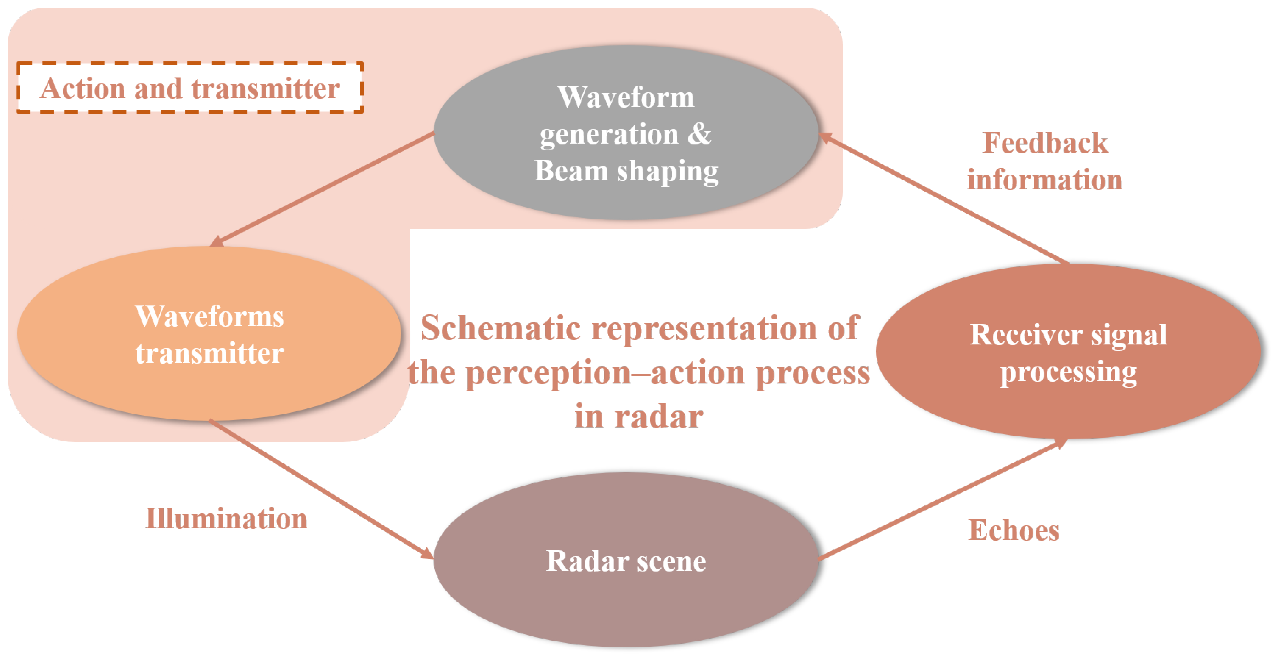
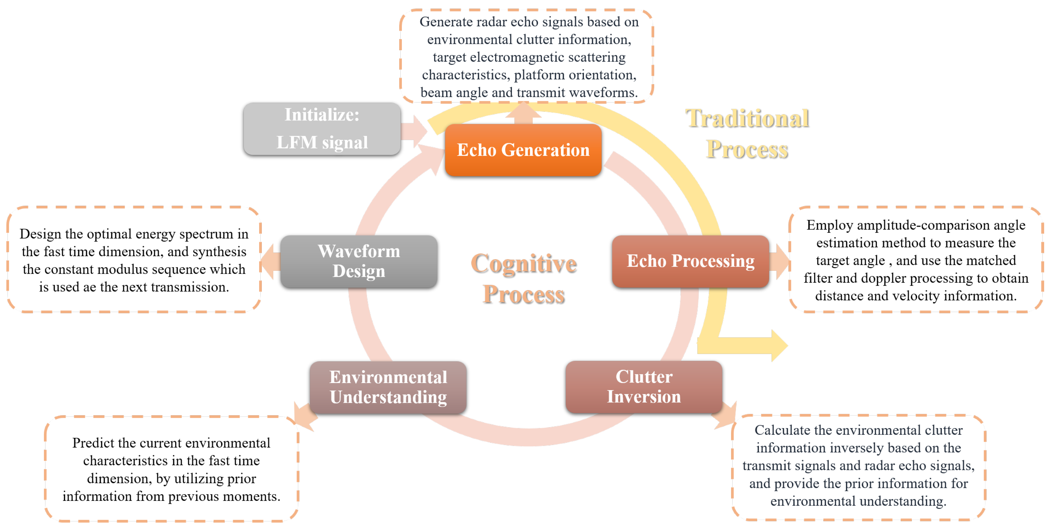
Waveform design plays an important role in CR from an application standpoint. Consequently, prior to explaining the proposed waveform method in this paper, we enhance the signal processing structure of traditional radar and propose a novel implementation strategy for the CR concept, as outlined in [38]. Figure 1 shows a flowchart that schematically represents the perception–action process proposed in [38]. Actually, the cognitive dynamic system mimics the human brain, reacting to the environment according to the basic perception–action cycle. The cycle consists of three basic components—executive, perception, and the environment—which correspond to the waveform transmitter, receiver signal processing, and radar scene in a radar system, respectively. We have refined the functions of each module based on the cognitive radar structure proposed in the literature, and designed corresponding signal processing and waveform design algorithms to preliminarily implement the closed-loop strategy of cognitive radar. Specifically, Figure 2 illustrates a flow chart comparing the signal processing procedures in a traditional radar system to those in a CR system. The procedure reveals that the transmission and receive filters of a traditional radar system operate independently, resulting in an open-loop mode for the system. Additionally, in the traditional radar signal processing procedure, the transmit waveform remains fixed and unchanging, preventing the system from utilizing environmental information from radar echoes as feedback for waveform adjustment.
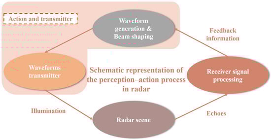
Figure 1.
Schematic representation of the perception–action process in a radar.
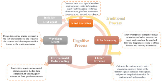
Figure 2.
Closed-loop cognitive strategy for CR.
To address the limitation of the traditional radar signal processing structure, a CR employs a dynamic closed-loop feedback structure for signal transmitting and receiving, allowing the radar system to perceive and comprehend the environment [39]. Building upon the fundamental principle of cognitive radar (CR), this paper introduces a novel closed-loop radar signal processing strategy. In terms of functionality, the closed-loop strategy consists of five parts, including echo generation, echo processing, clutter inversion, environmental understanding, and waveform design. The proposed method in this paper is employed in the waveform design module, which plays an important role in the CR system.
In the first stage, the system is initialized by the LFM transmit signal. Afterward, the echo generation module calculates the radar echo by considering the real-measured clutter data, target radar cross-section, transmit waveform, and geometric relationship between the platform, target, and the surrounding environment. Then, the echo is analyzed by the echo processing module, which aims to obtain information on the target distance from the platform and the target velocity relative to the platform. The algorithm employed in this module utilizes traditional radar signal processing methods. For instance, in this experiment, matched filtering is employed for distance measurements, whereas moving target detection is utilized for speed measurements.
The above-mentioned two modules are commonly used structures in open-loop radar systems. This paper proposes a closed-loop strategy, in which the radar echo is utilized to provide feedback to the transmit module. Specifically, the clutter inversion module inverts the environmental information from the previous moment. The environmental understanding model uses the previous clutter spectrum as prior information and predicts the information in the next moment. Finally, the proposed waveform design method is employed in the waveform design module, synthesizing the CM sequence. The sequence is transmitted by the radar front-end instead of the LFM signal, and then the radar system enters the next cycle.
3. Waveform Design Method Signal Model and Problem Formulation
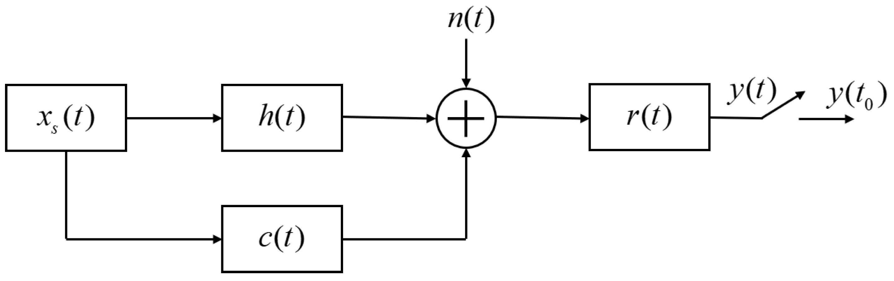
In the context of CR waveform design for a monostatic radar system, Figure 3 shows the signal model of waveform design in signal-dependent interference, where is the transmit signal, is the target impulse response, represents the clutter, represents the noise, and denotes the receiver filter. We define the spectrum of the transmit waveform as . Then, according to the Cauchy–Schwartz inequality, the maximum value of the output SINR in can be computed as
where , is the PSD of additive Gaussian white noise (AGWN), is the clutter PSD, and and denote the Fourier transform of the target pulse response and the receive filter.
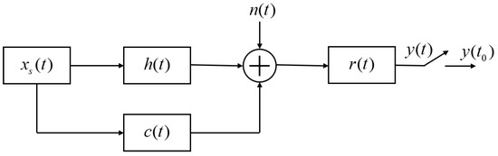
Figure 3.
Signal model of waveform design in signal-dependent interference.
Equation (1) is a classical waveform design metric widely used in many studies [33,35]. However, the derivation process of the SINR expression contains some reasonable approximations aimed at deriving the analytical solution of the waveform’s optimal energy spectrum. This causes the metric (1) to be an upper bound for the SINR if and only if takes on a specific form. In practical scenarios, the expression of the SINR should be the ratio of two integration results, and the expression in Equation (1) is not accurate enough. Thus, we derive a corrected SINR expression for signal-dependent interference in the frequency domain below.
According to Pazwal’s theorem [40], the energy of the target echo and interference (clutter plus noise) can be computed as
and
Thus, the corrected SINR in the frequency domain can be calculated as
where W is the bandwidth of the transmit waveform.
Although the WF method performs well in terms of the SINR, it may distribute a large amount of energy to several frequency points with a high target response. This phenomenon causes some undesirable properties of the waveform, such as low bandwidth, poor distance resolution, and high ISL. To address this issue, an equivalent bandwidth constraint, which can also be referred to as a delay resolution constant, is incorporated into our optimization model. Specifically, Woodward proposed a characteristic radar parameter in [41], known as the time-delay resolution constant . This parameter takes into account the levels of both the main lobe and the sidelobes, providing an indication of the resolution characteristics. The detailed expression of can be given as
where is defined as the equivalent bandwidth, and
where is the ambiguity function (AF) of the transmit signal , which represents the ability of the waveform to resolve two targets with a time-delay difference of and a Doppler frequency difference of .
For two targets with an identical velocity to the radar system, the ACF can be defined as
Hence, according to Pasval’s theorem, Equation (3) can be rewritten in the frequency domain as
Above all, a waveform design model with energy and bandwidth constraints is presented in this paper as
where and denote the defined waveform energy and time-delay resolution constant, respectively. In addition, the time-delay resolution constant constraint is referred to as the bandwidth constraint in the following section for ease of understanding.
4. Joint Constraints Waveform Spectrum Design Algorithm and Time Synthesis Method
4.1. Joint Constraints Waveform Spectrum Design Algorithm
Since the optimization problem (5) with integral symbols is difficult to solve, we transform it into a discrete form in this subsection. Suppose that is the square of the amplitude value of the target frequency response, which is the discrete form of . is the ESD of the transmit waveform, which is the discrete form of . Additionally, and refer to the PSD values of the clutter and noise, which can be denoted as and , respectively. Therefore, (5) can be rewritten as
where , and is the frequency resolution. Since the optimal model (6) is a nonlinear fractional programming problem, its functions established via the KKT condition are hard to solve. Therefore, we take the logarithm of the objective function and convert it into its first-order Taylor expansion at point , which is in close proximity to the optimal solution . The first-order Taylor expansion of can be expressed as
where and are constants. Hence, the objective function of (6) can be reformulated as minimizing , thereby transforming the non-convex problem into a convex problem. It is widely known that if a strong duality relationship exists between the original problem and the dual problem, the solution to the Karush–Kuhn–Tucker (KKT) condition is the optimal solution to the optimal problem, and the Slater condition is used to determine if the strong duality holds. In cases where the original problem is convex and the Slater condition holds, the strong duality holds. The optimal solution found to prove the Slater conditions is the vector , where each element equals . Then, the optimal solution to the original function can be acquired by solving the KKT conditions. The functions established by the KKT conditions are expressed as
where , , μ are Lagrange multipliers.
Theorem 1.
The results of the functions established by the KKT conditions are
where
are element-wise operations
and means the positive value. The proof process is as follows.
Proof of Theorem 1.
b. For the case where , must hold to satisfy condition (12). □
Specifically, the method for computing is outlined in Algorithm 1, where is the search step size of variable , j is the iteration time, and e is the iteration error. The criterion for the convergence of Algorithm 1 is set at an iteration error of . Furthermore, the computational complexities of both the proposed method and the water-filling method are analyzed. The computational complexity of the proposed method is , whereas the computational complexity of the water-filling method is . Actually, the foundations of both methods are analytical expressions. However, because of the difference in the number of constraints, the water-filling method has one parameter to solve, whereas the proposed method has two. Hence, the proposed method has higher computational complexity than the water-filling method since it proposes both a high SINR and a high equivalent bandwidth.
| Algorithm 1 Joint Constraints Waveform Spectrum Design |
| Input: , , , , Output: , , , e |
4.2. CM Sequence Synthesizing for Optimal Frequency Spectrum
In the previous subsection, the ESD of the optimal waveform was obtained. Subsequently, a time-synthesizing algorithm should be used to make sure of its CM property in the time domain [42]. Given that is an n-point unit-amplitude complex time domain signal, is its corresponding Fourier transform, and its amplitude should be close to ϵ. This can be easily obtained by minimizing the following least squares error
where ϕ is the phase of . The least squares error can be represented as
where . is an discrete Fourier transform (DFT) matrix defined as
The linear least squares estimator of is
As depends on the phase , the problem should be solved iteratively. The process for obtaining the time synthesis signal is summarized in Algorithm 2, where k is the iteration time. The criterion for the convergence of Algorithm 2 is set as the norm of the difference vector between the results of two consecutive iterations being less than .
| Algorithm 2 An iterative method for the time synthesis signal |
| Input: ϵ Output: ϕ
|
5. Experiments and Analysis
In this section, simulation experiments are performed to verify the superior performance of the proposed algorithm. Furthermore, real-measured ground clutter data and real target radar cross-section (RCS) frequency responses are subsequently introduced as clutter PSD and target ESD to enhance the credibility of the experiments. Specifically, Experiment 1 demonstrates the enhancement of the SINR after correcting the optimization metric; Experiment 2 shows the effectiveness of the joint constraints waveform design method and time synthesis algorithm; Experiment 3 proves the outstanding performance of the designed waveform in terms of the ISL metric; Experiment 4 discusses the relationships among the transmit energy, bandwidth, and SINR; Experiment 5 verifies the algorithm using real-measured data; and finally, the proposed waveform design is applied in the closed-loop strategy in Experiment 6 to test its application in cognitive radar.
Implementation Details: Our proposed method is compared to the WF method in [33] and the linear frequency-modulated (LFM) signal in the following subsection. Additionally, we define the target-to-clutter ratio (TCR) as the area under the target power spectrum to the area under the clutter PSD, and we define the clutter-to-noise ratio (CNR) as the area under the clutter PSD compared to the noise PSD. In the following experiments, we set both the TCR and CNR to 0 dB, meaning that the energies of the target, clutter, and noise are the same [33]. Moreover, all experiments are implemented in MATLAB R2022b and run on a PC with a 2.30 GHz i7-12700H CPU and 16 GB of RAM.
5.1. Experiment 1: Correct SINR Metric without Bandwidth Constraint
Simulation Scenario: The simulation experiment scenario simulates the detection of a stationary target from a stationary platform. Regarding the radar parameters, the bandwidth is 50MHz, and the signal pulse width is 2.5 s. Regarding the target and interference model, we assume that the clutter and target consist of several Gaussian spectra. Specifically, the target frequency response can be expressed as
where is the number of frequency points with a higher target response, and , , and are the weight, variance, and center frequency of each target Gaussian spectrum, respectively. The target frequency response is set to Gaussian spectrum superimposed, and the parameters for each Gaussian spectrum are shown in Table 1.

Table 1.
Parameters of each Gaussian spectrum in the target frequency response.
The interference in the simulation model is composed of ambient clutter and noise. The clutter PSD can be represented in a similar form, as
where is the number of frequency points with a higher clutter response, and , , and are the weight, variance, and center frequency of each clutter Gaussian spectrum. The parameters of the clutter spectrum are , , = 8.3 × 10, 8.3 × 10, and . The noise is assumed to be additive white Gaussian noise with a flat PSD, which is .
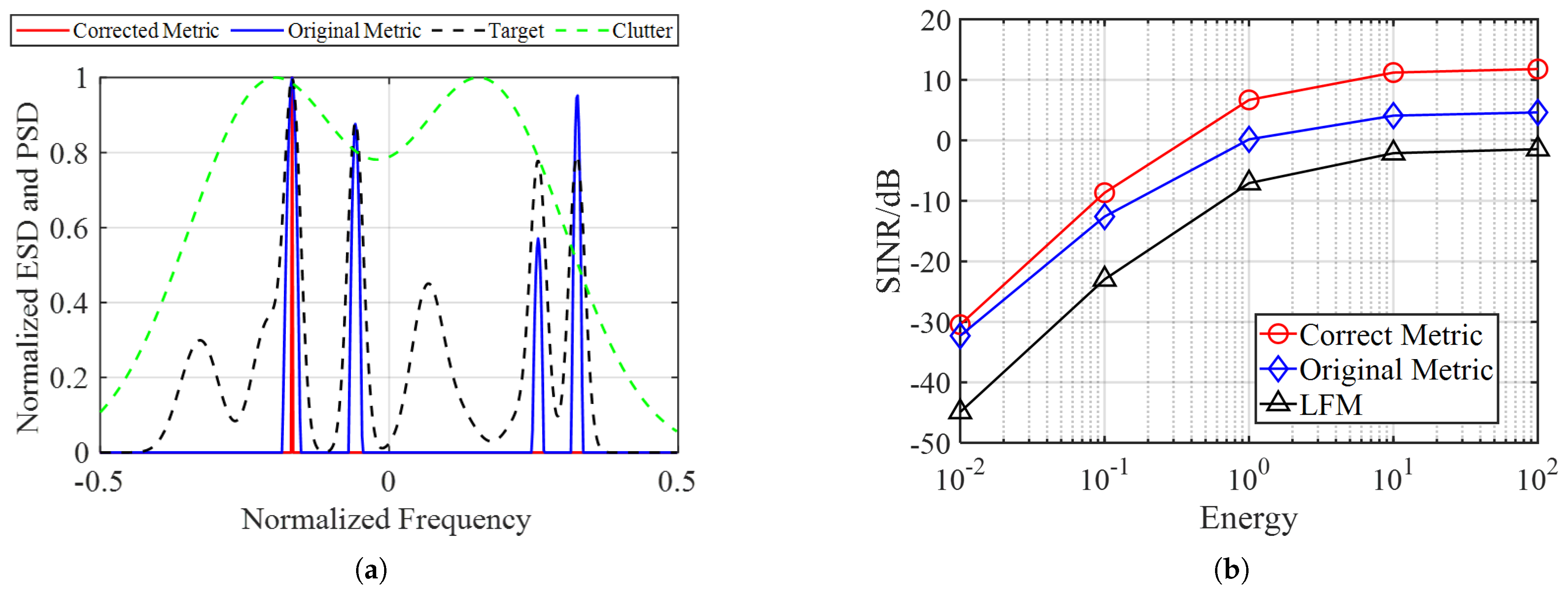
The SINR performance of the waveform design results without an equivalent bandwidth constraint is investigated in this subsection. By comparing the waveforms obtained using different objective functions (1) and (2), we can assess the outcome of our waveform design method, as shown in Figure 4a. The Correct Metric represents the result of objective function (2), whereas the Original Metric represents the result of objective function (1). The results demonstrate that our proposed metric leads to a more centralized energy distribution. Specifically, the WF waveform has four peaks, whereas the waveform designed using the corrected metric has only one peak. This is because the SINR expression has been changed from function (1), which involves the integral of the ratio, to function (2), which is the ratio of two integrals. This change in expression causes the energy of the other three peaks in the original waveform to transfer to one point, which has the highest signal-to-clutter ratio, in the proposed waveform. Moreover, the SINR of the waveform in the red line spectrum aligns better with our measurement standard and is numerically higher. This is why the waveform designed using the corrected metric only has one peak.

Figure 4.
Performance of waveform without bandwidth constraints, original WF waveform, and the LFM signal. (a) Clutter PSD, target ESD, and waveform spectrum design results. (b) SINR performance varying with the transmit energy.
Then, we compare the SINR performance of waveforms under different metrics. The waveform energy is set at 1 × 10 to 1 × 10, and the outcome is shown in Figure 4b, demonstrating that the SINR performance improved compared to the other two kinds of waveforms using the corrected metric. However, it can be seen that the low bandwidth is indeed a disadvantage brought about by correcting the objective function of the water-filling method. Hence, the bandwidth constraint is introduced in the following experiments.
5.2. Experiment 2: Correct SINR Metric with Bandwidth Constraint
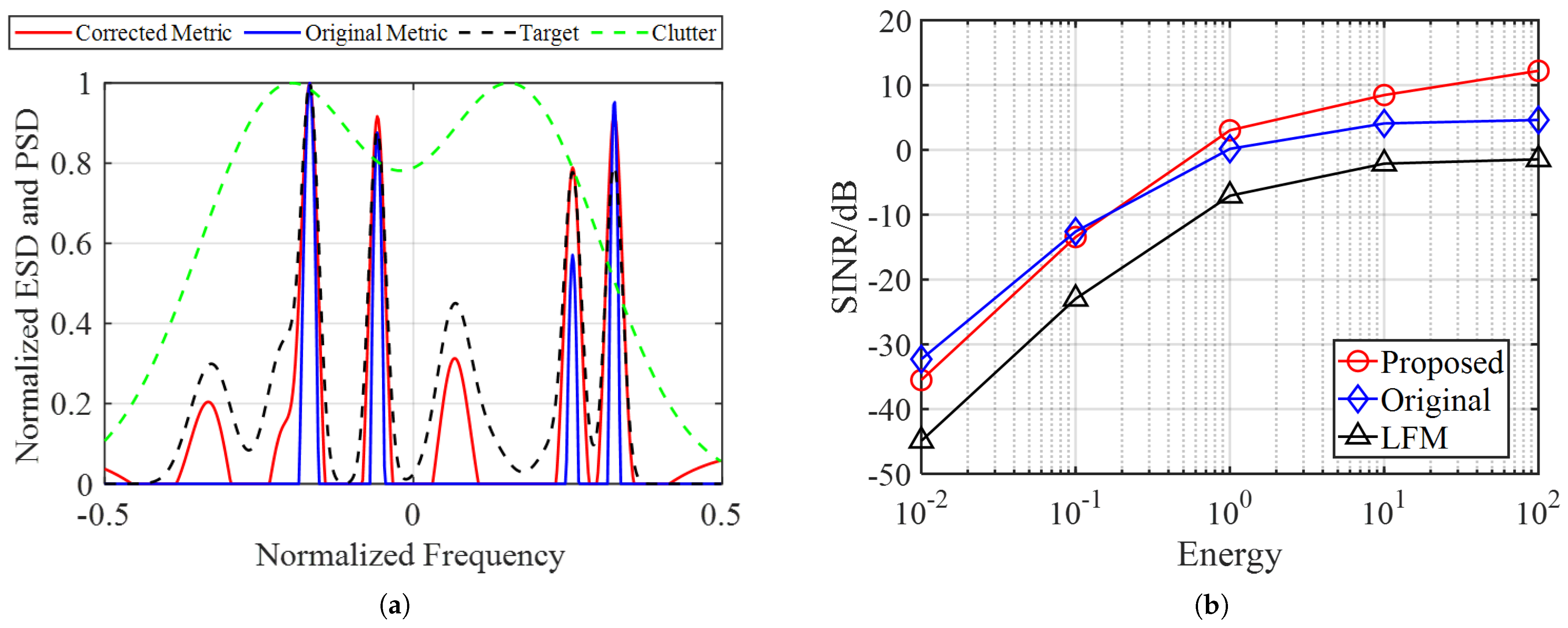
Algorithms 1 and 2 are verified in this subsection. Figure 5a compares the waveform design results of the proposed method with the original WF method, where Proposed represents the joint constraints algorithm and Original represents the original method. The transmitted energy is set to 1 × 10, and the equivalent bandwidth is set to . Moreover, the equivalent bandwidth of the WF waveform is 0.075.
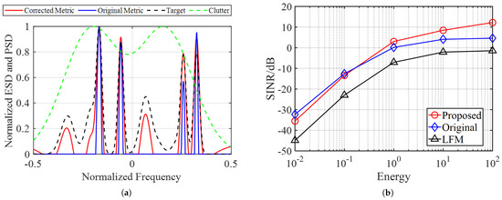
Figure 5.
Performance of waveform under joint constraints, original WF waveform, and the LFM signal. (a) Clutter PSD, target ESD, and waveform spectrum design results. (b) SINR performance varying with the transmit energy.
As illustrated in the previous subsection, the transmit energy varied from 1 × 10 to 1 × 10. An interesting phenomenon can be seen in Figure 5b, revealing that the output SINR of the waveform under joint constraints is lower than that of the original WF waveform when is low. In particular, around 1 × 10 is the critical energy at which the SINR and equivalent bandwidth of both waveform design methods are approximately equal. However, when the waveform energy increases, the SINR of the proposed method surpasses that of the original method. This can be explained by the fact that when the transmitted energy is low, the bandwidth of the water-filling waveform is smaller than 0.25, and the energy allocation strategy of the proposed method is affected by the bandwidth constraint, which causes the loss of the SINR. When the transmit energy increases, the bandwidth of the water-filling waveform is larger than 0.25, and the proposed method tends to concentrate the energy at several frequency points with a higher response, resulting in a higher SINR, just as in Experiment 1.
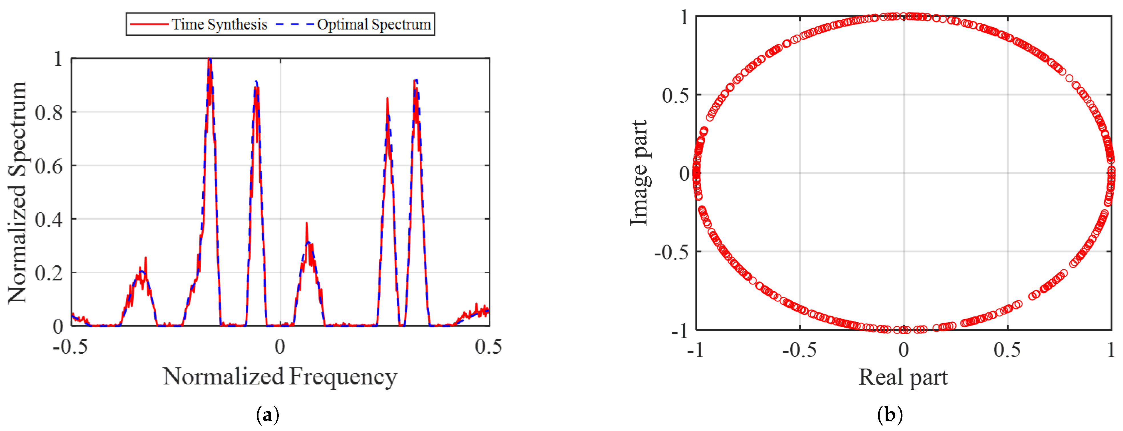
Furthermore, Figure 6a illustrates the spectra of the time synthesis waveform and the corresponding optimal waveform, providing evidence for the effectiveness of the time synthesis algorithm. Figure 6b indicates that the time synthesis waveform possesses the CM property.
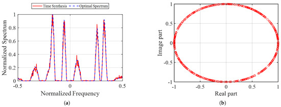
Figure 6.
ESD, real, and imaginary parts of time synthesis waveform. (a) Spectrum of time synthesis waveform and optimal spectrum. (b) Real and imaginary parts of time synthesis waveform.
5.3. Experiment 3: ISL Metric of Waveform under Joint Constraints
Assume that
is the correlation function of the transmit sequence . Then, the ISL metric of the waveform can be expressed as
The expression of the Merit Factor (MF) can be written as
The MF metric has been commonly employed to assess the sidelobe levels of waveforms in prior research [43], as the minimization of the ISL is equivalent to the maximization of the MF. At the same time, unimodular sequences with high MF values are essential in radar systems and wireless communication due to their excellent anti-clutter performance. As previously mentioned, the MF metric is equivalent to the concept of the equivalent bandwidth [37]. Therefore, in this subsection, we compare the ISL performance, specifically the MF value, of the sequences designed using the proposed and the original WF methods.
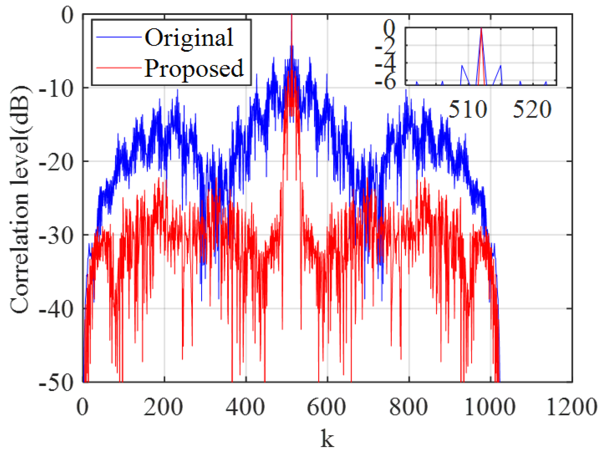
In this experiment, the transmit waveform energy is set to 1 × 10, and the equivalent bandwidth is set to . Figure 7 shows a comparison of the correlation level of the sequences designed using the proposed and original methods. Both of the sequences are CM and generated using Algorithm 2. It can be seen in Figure 7 that the waveform designed under the equivalent constraint exhibits a lower sidelobe level compared to the original WF waveform. Table 2 shows the MF values of the sequences under different equivalent bandwidth constraints when the transmit energy is set to 1 × 10. Since the transmit energy is fixed, the sequence designed using the WF method is the same under different equivalent bandwidths, whereas the MF value of the sequence designed using the proposed method increases with the equivalent bandwidth. Moreover, the sequences designed using the proposed method exhibit significantly higher MF values compared to those designed using the WF method.

Figure 7.
Correlation levels of the sequences designed using the proposed method and the original WF method.
Table 2.
MF values of the sequence designed using the proposed method ( 1 × 10).
5.4. Experiment 4: Relationships among the Transmit Energy, Bandwidth, and SINR
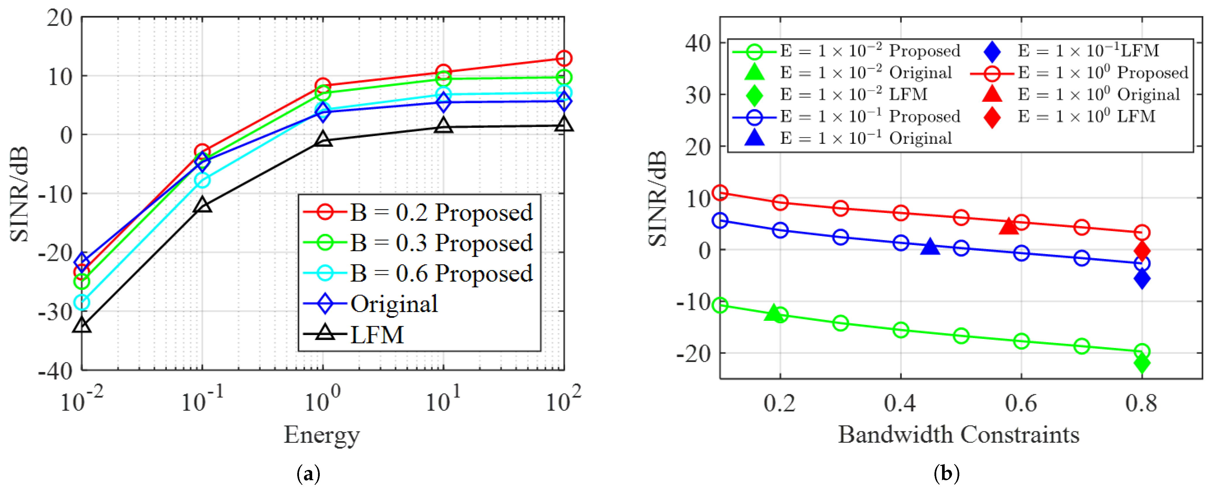
The relationships among the transmit signal energy, bandwidth, and SINR are further investigated, as shown in Figure 8. Figure 8a shows a comparison of the SINR performance of the waveforms designed under different equivalent bandwidth constraints, and Figure 8b shows a comparison of the SINR performance of the waveforms designed under different energy constraints. As shown in Figure 8a, it is evident that the SINRs of the waveforms designed using the proposed method gradually increase as the equivalent bandwidth constraints decrease. Figure 8b shows the trends of the SINR performance, which gradually deteriorates as the equivalent bandwidth increases.
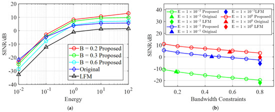
Figure 8.
Relationships among the SINR, equivalent bandwidth, and transmit energy. (a) SINR performance under different equivalent bandwidth constraints. (b) SINR performance under different transmit energy constraints.
5.5. Experiment 5: Application of the Waveform Design Method to a Stationary Platform Using Real-Measured Data
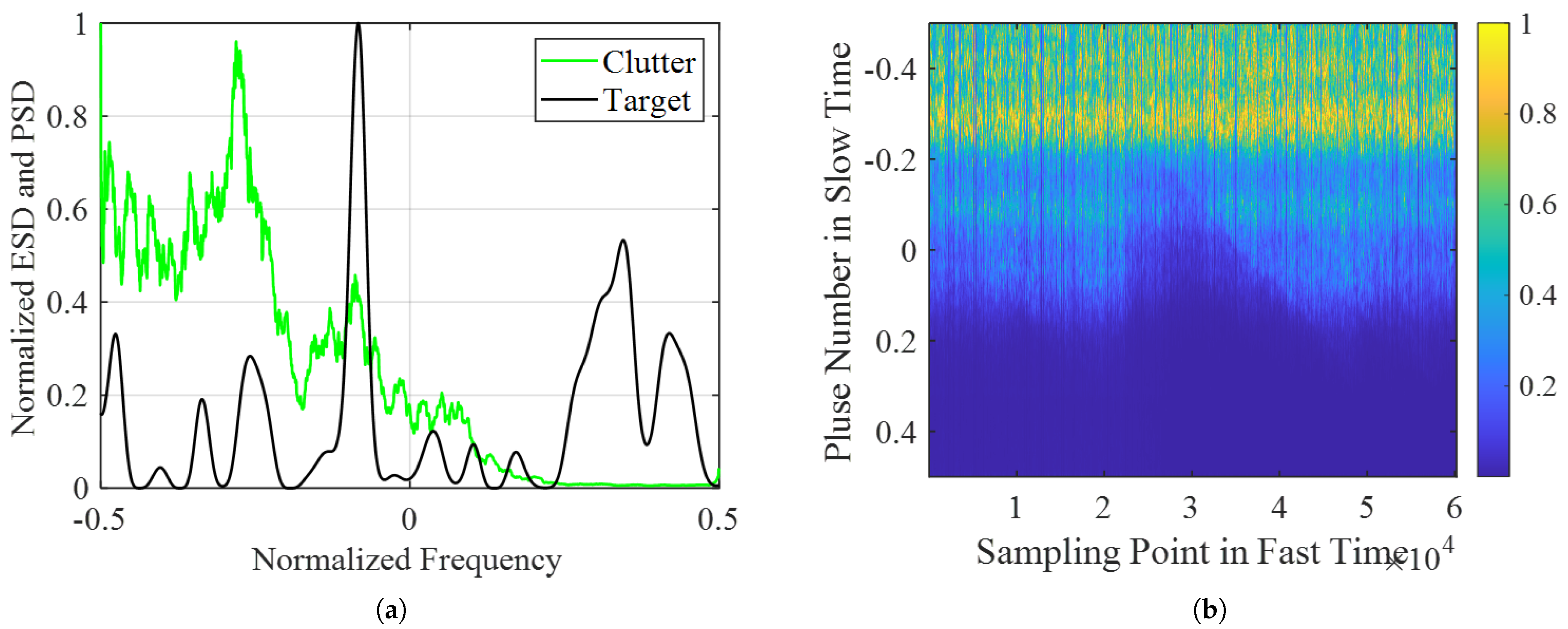
To enhance the credibility of the experiments, the real-measured environmental data and target data are utilized to assess the effectiveness of the proposed method on a stationary platform. The real-measured clutter data presented in this and the next subsections were acquired in a region of Hainan, China, and the acquisition conditions are presented in Table 3. The target is an armored vehicle with pitch and azimuth angles identical to those of the ground clutter. Since the number of samples for the target RCS is considerably fewer than the number of PSD values for the clutter within the same bandwidth, we interpolate each frequency point of the target for a more accurate analysis. It can be seen in Figure 9 that the clutter energy is concentrated in the normalized frequency range of , whereas the target frequency response is large at several specific frequency points.
Table 3.
Ground clutter acquisition radar parameters.
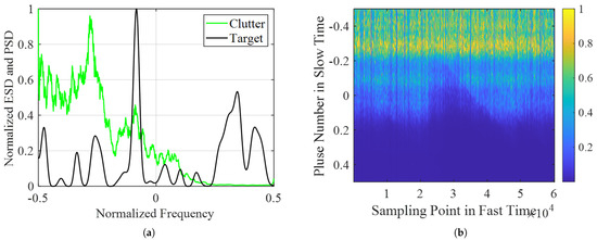
Figure 9.
PSD of real-measured clutter. (a) Clutter PSD in different PRTs. (b) Real-measured clutter PSD and target ESD.
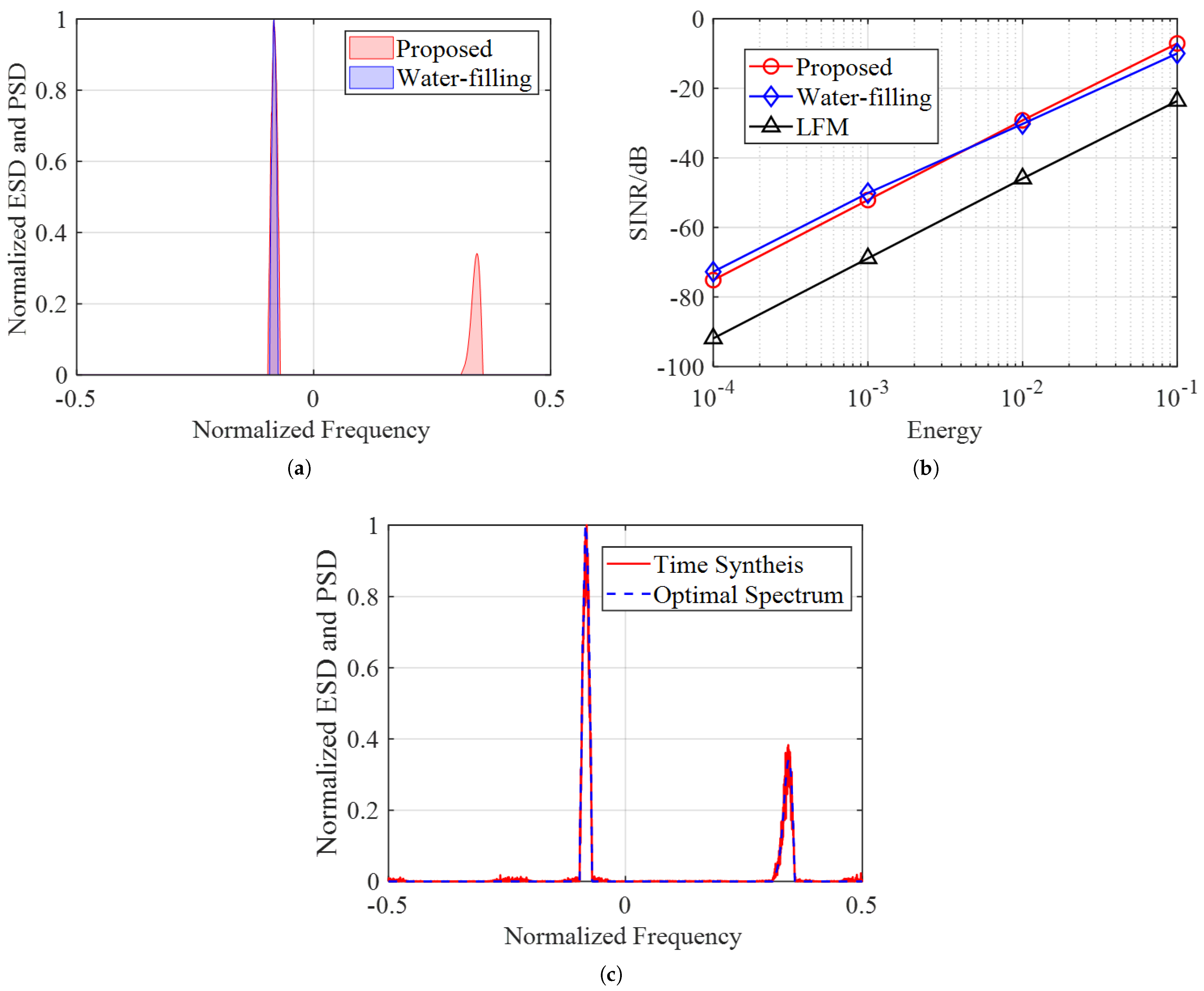
In the following real-measured experiments, the energy of the transmit signal is set to 1 × 10, and the equivalent bandwidth constraint in the proposed method is set to . The optimal waveform spectrum, corresponding time-synthesized sequences, and their performance are illustrated in Figure 10. Figure 10a shows the optimal spectra of the proposed method and WF method. It can be seen that the proposed algorithm is designed to distribute the waveform energy spectrum more evenly compared to traditional methods. After calculation, the equivalent bandwidths of the proposed method and original method are 0.1 and 0.02, respectively. Figure 10b demonstrates the superior performance of the proposed algorithm compared to the WF method and LFM signal, and Figure 10c shows the time-synthesized signal results.
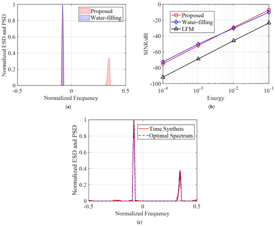
Figure 10.
Results of real-measured data. (a) Proposed and original waveform spectrum design results. (b) SINR performance varying with the transmit energy. (c) Spectrum of time synthesis waveform and optimal spectrum.
5.6. Experiment 6: Application of Waveform Design Method in the Closed-Loop CR Strategy
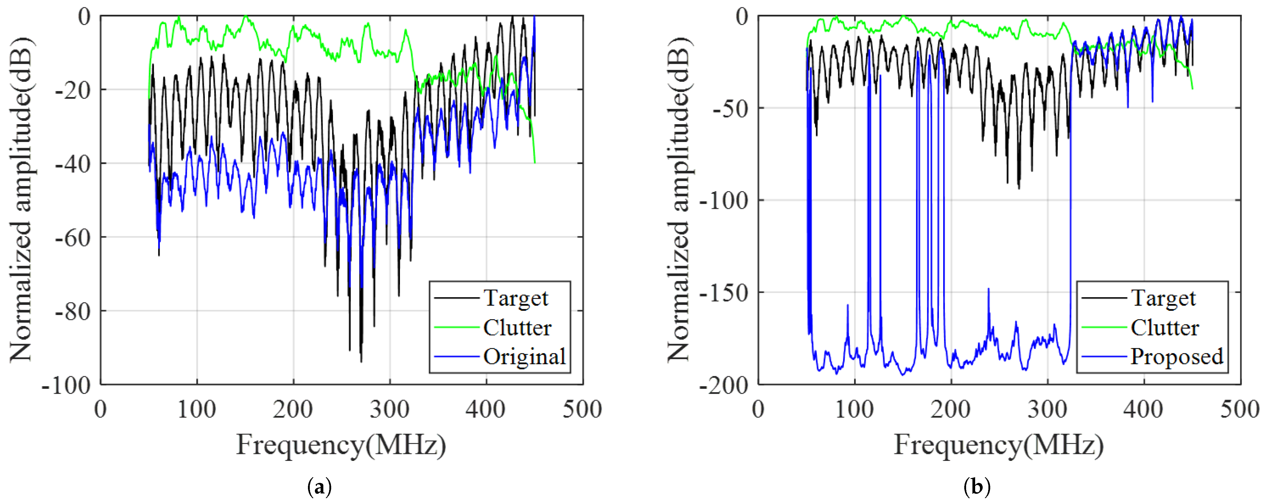
To provide a deeper understanding of the impact of the proposed waveform design method, this subsection uses the closed-loop CR strategy mentioned above to evaluate its performance in a CR system application. Regarding the data, another set of real-measured data is used in this subsection as prior clutter information to test the performance of our algorithm in the closed-loop cognitive strategy. There are three sets of experiments using a traditional process with an LFM signal and a cognitive process with different transmit waveforms. Since the cognitive process is initialized by the LFM transmit signal, the following cognitive process figures display the corresponding results in the second PRT instead of the first one. Figure 11 displays the optimal waveform using different waveform design methods. It can be seen that the target frequency response is high in the low- and high-frequency bands, whereas the clutter energy spectrum is high in the low-frequency band. When comparing Figure 11b and Figure 11a, it can be seen that the proposed method ensures that the optimal energy spectrum focuses on the high-frequency band and aligns with the target frequency response at some frequency points. Specifically, the equivalent bandwidth of the WF method is MHz, whereas the equivalent bandwidth of the proposed method is MHz.
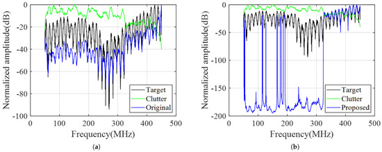
Figure 11.
Radar optimal spectrum using different methods. (a) WF method. (b) Proposed method.
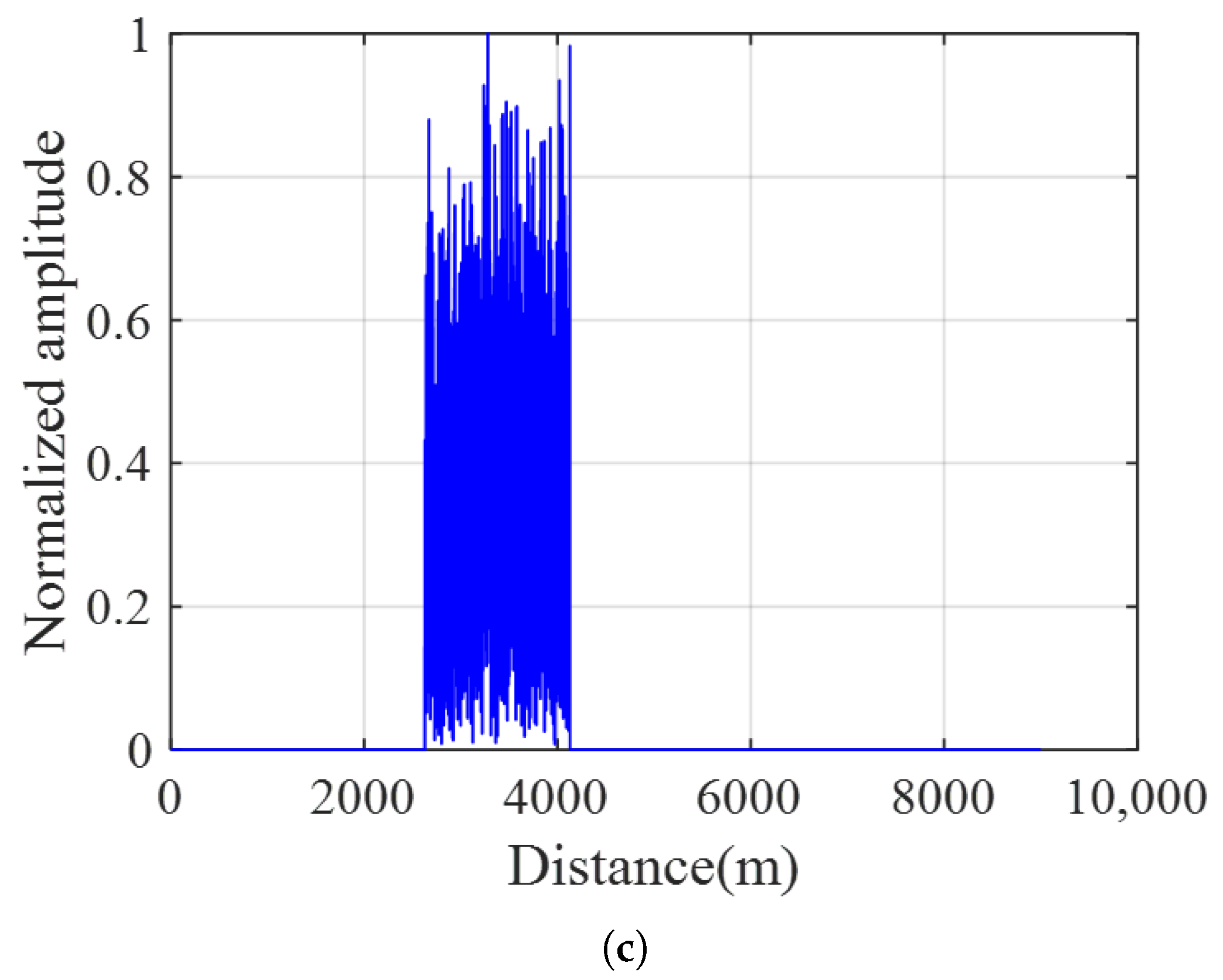
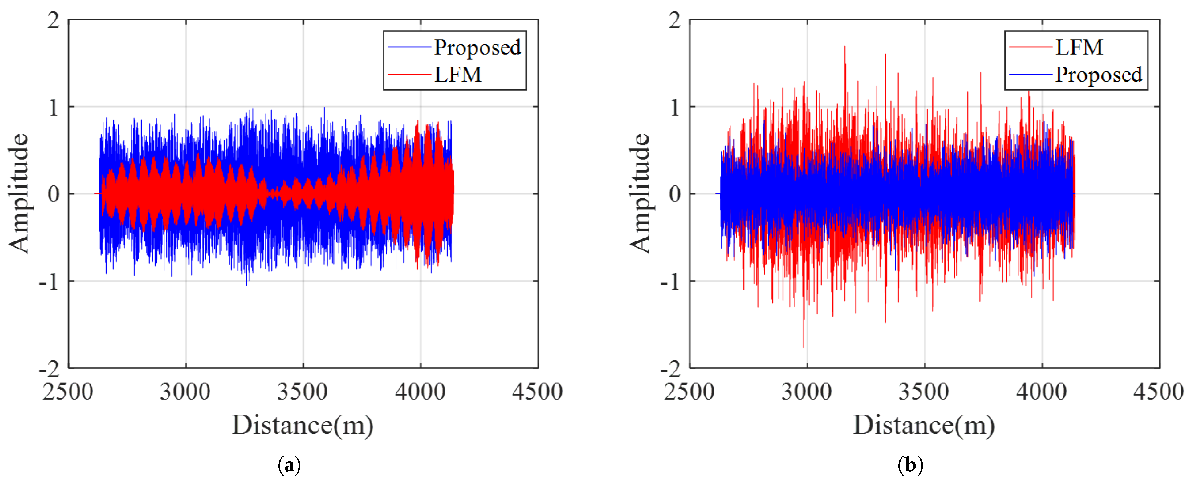
The following figures illustrate the clutter suppression and target enhancement achieved using the proposed method. Figure 12 illustrates the radar echo in one PRT under different transmit waveforms, which can be considered to be composed of three parts: target echo, clutter echo, and noise according to Figure 3. More specifically, Figure 13a,b display the separate echoes of the target and clutter, respectively, when the transmit signal is an LFM signal and the waveform is designed using the proposed method. The blue line is the echo of the designed waveform, and the red line is the LFM signal. The results show that after optimizing the spectrum of the transmit waveform, the target echo is enhanced to twice its previous level, and the clutter echo is reduced to half its previous level. The enhancement of the target echo energy and the attenuation of the clutter echo energy demonstrate the outstanding performance of the designed waveform in improving the output SINR.
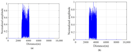

Figure 12.
Radar echo synthesized by the echo generation module in one PRT under different transmit waveforms. (a) LFM signal. (b) Waveform designed using the WF method. (c) Waveform designed using the proposed method.
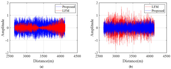
Figure 13.
Echo within the pulse width under different transmit waveforms. (a) Target echo. (b) Clutter echo.
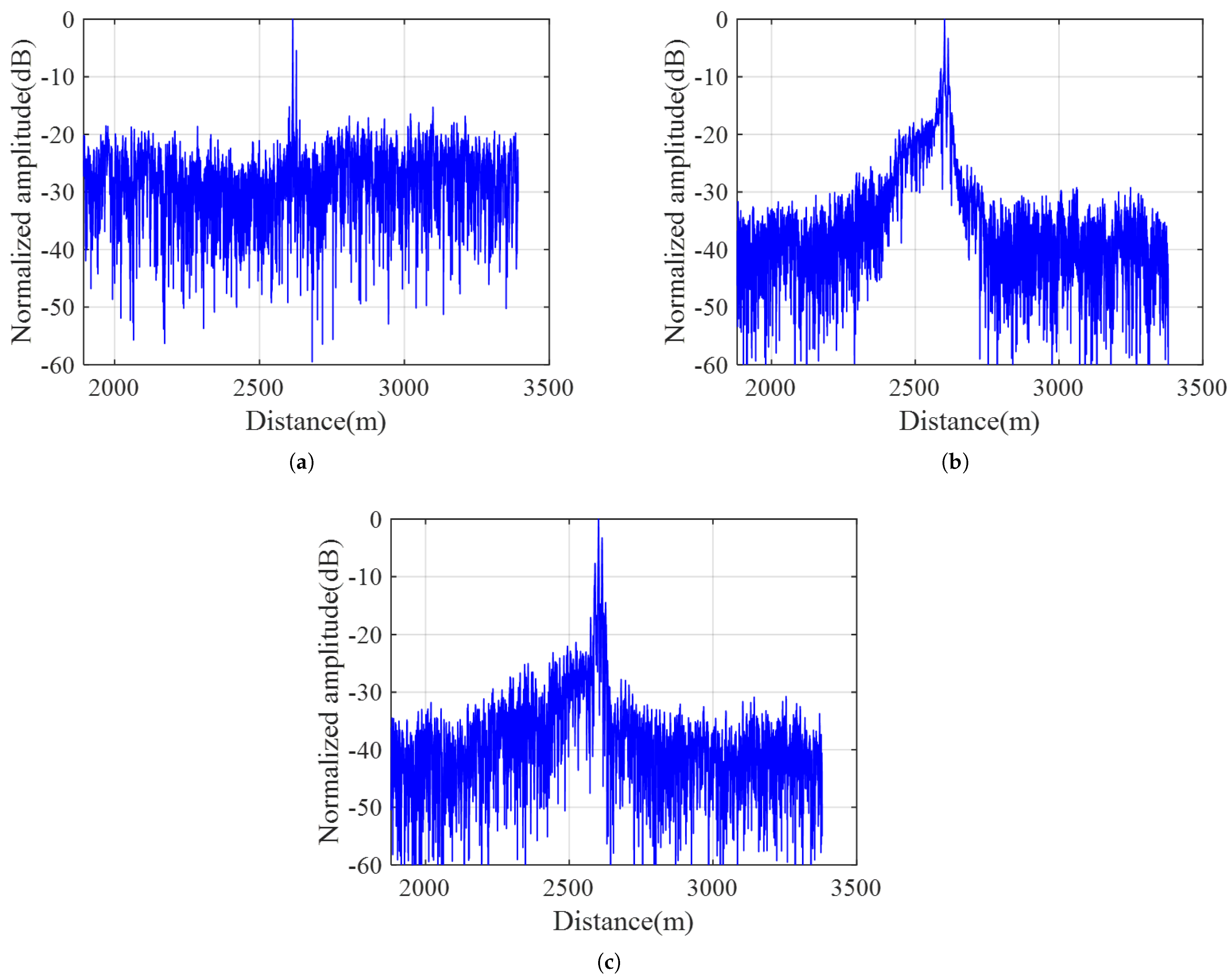
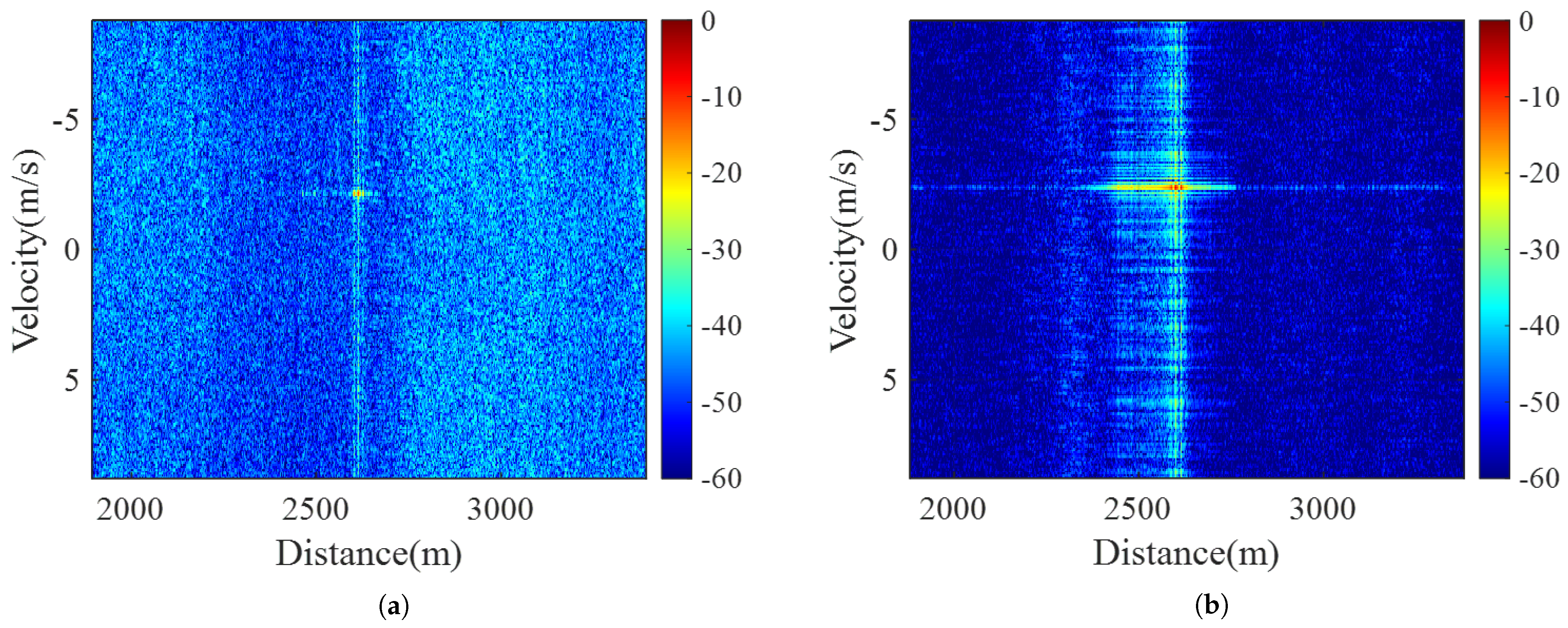
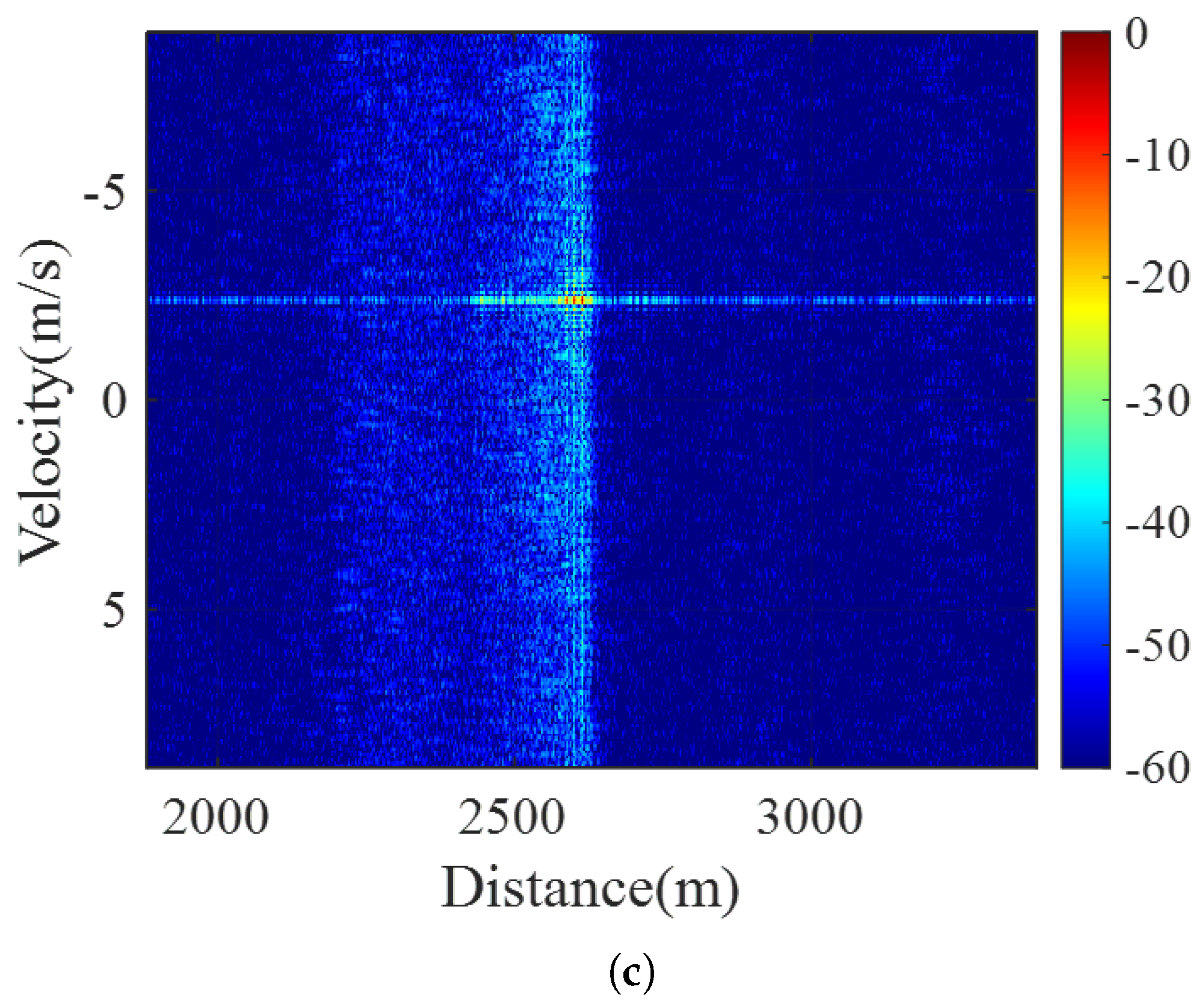
Figure 14 and Figure 15 illustrate the output of the echo processing module. In Figure 14, it can be observed that the sidelobe level of the LFM transmitting waveform is −20 dB, whereas the sidelobe levels of the waveforms designed using the WF method and the proposed method are about −30 dB. Meanwhile, the sidelobe of the proposed waveform is lower than that of the WF waveform. Figure 15 shows the range-Doppler image of the radar echo. As the transmit waveform changes from the LFM signal to the optimal waveform, the target becomes more prominent in the clutter, and the detection difficulty decreases.

Figure 14.
Matched filter results under different transmit waveforms. (a) LFM signal. (b) Waveform designed using the WF method. (c) Waveform designed using the proposed method.
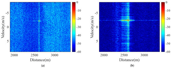
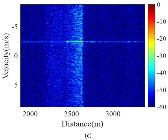
Figure 15.
Range-Doppler results under different transmit waveforms. (a) LFM signal. (b) Waveform designed using the WF method. (c) Waveform designed using the proposed method.
6. Conclusions
In this paper, we address the issue of the low-distance resolution of the traditional WF waveform by proposing a novel waveform design model that contains both energy and equivalent bandwidth constraints. Specifically, we follow two steps to obtain the optimal transmit waveform in the time domain. First, the KKT conditions are employed to solve the non-convex problem and optimize the waveform energy spectrum. Then, a time synthesis method is used to synthesize the unimodular sequence in the time domain. To demonstrate the effectiveness of our proposed approach, experiments using simulation and real-measured data are conducted to verify that the proposed method can enhance the equivalent bandwidth of the WF waveform while maintaining superior SINR performance. Finally, to verify the practical application value of the proposed waveform design method, a closed-loop CR strategy is proposed, and the results of the experiments under real-measured data illustrate the superior performance of this strategy in comparison to traditional radars.
Author Contributions
Conceptualization, C.Y. and W.Y.; methodology, C.Y. and W.Y.; software, C.Y. and X.Q.; validation, C.Y. and W.Y.; formal analysis, C.Y. and W.Y.; writing—original draft preparation, C.Y.; writing—review and editing, C.Y., W.Y., X.Q., W.Z., Z.L. and W.J.; supervision, W.Y. and W.J. All authors have read and agreed to the published version of the manuscript.
Funding
This research was funded by the National Natural Science Foundation of China under grant numbers 61871384, 61901487, 61901498, and 61921001, and the Science and Technology Innovation Program of Hunan Province under grant number 2022RC1092.
Data Availability Statement
Not applicable.
Conflicts of Interest
The authors declare no conflict of interest.
References
- Gurbuz, S.Z.; Griffiths, H.D.; Charlish, A.; Rangaswamy, M.; Greco, M.S.; Bell, K. An Overview of Cognitive Radar: Past, Present, and Future. IEEE Aerosp. Electron. Syst. Mag. 2019, 34, 6–18. [Google Scholar] [CrossRef]
- He, H.; Li, J.; Stocia, P. Waveform Design for Active Sensing Systems: A Computational Approach; Cambridge University Press: Cambridge, UK, 2012. [Google Scholar]
- Aubry, A.; De Maio, A.; Jiang, B.; Zhang, S. Ambiguity function shaping for cognitive radar via complex quartic optimization. IEEE Trans. Sig. Process. 2013, 61, 5603–5619. [Google Scholar] [CrossRef]
- Bu, Y.; Yu, X.; Yang, J.; Fan, T.; Cui, G. A new approach for design of constant modulus discrete phase radar waveform with low WISL. Sig. Process. 2021, 187, 108145. [Google Scholar] [CrossRef]
- Song, J.; Babu, P.; Palomar, D.P. Sequence design to minimize the weighted integrated and peak sidelobe levels. IEEE Trans. Sig. Process. 2015, 64, 2051–2064. [Google Scholar] [CrossRef]
- Wu, L.; Babu, P.; Palomar, D.P. Cognitive radar-based sequence design via SINR maximization. IEEE Trans. Sig. Process. 2016, 65, 779–793. [Google Scholar] [CrossRef]
- Zhang, H.; Zhang, W.; Liu, Y.; Yang, W.; Yong, S. Scatterer-Level Time-Frequency-Frequency Rate Representation for Micro-Motion Identification. Remote Sens. 2023, 6615, 4917. [Google Scholar] [CrossRef]
- Zhang, H.; Tang, M.; Zhang, W.; Yang, W.; Jiang, W. Micro-motion Signal Enhancement via Convolutional Autoencoder Equipped with Multi-scale Feature Pyramid. In Proceedings of the 2023 8th International Conference on Signal and Image Processing (ICSIP), Wuxi, China, 8–10 July 2023; pp. 758–762. [Google Scholar]
- Wu, L.; Babu, P.; Palomar, D.P. Transmit waveform/receive filter design for MIMO radar with multiple waveform constraints. IEEE Trans. Sig. Process. 2017, 66, 1526–1540. [Google Scholar] [CrossRef]
- Zhao, L.; Sone, J.; Babu, P. A unified framework for low autocorrelation sequence design via majorization–minimization. IEEE Trans. Sig. Process. 2016, 65, 438–453. [Google Scholar] [CrossRef]
- Tang, B.; Naghsh, M.M.; Tang, J. Relative Entropy-Based Waveform Design for MIMO Radar Detection in the Presence of Clutter and Interference. IEEE Trans. Sig. Process. 2015, 63, 3783–3796. [Google Scholar] [CrossRef]
- Sun, Y.; Babu, P.; Palomar, D.P. Majorization-minimization algorithms in signal processing, communications, and machine learning. IEEE Trans. Sig. Process. 2016, 65, 794–816. [Google Scholar] [CrossRef]
- Zhou, K.; Quan, S.; Li, D.; Liu, T.; He, F.; Su, Y. Waveform and Filter Joint Design Method for Pulse Compression Sidelobe Reduction. IEEE Trans. Geosci. Remote Sens. 2022, 60, 1–15. [Google Scholar] [CrossRef]
- Li, Y.; Vorobyov, S.A. Fast Algorithms for Designing Unimodular Waveform(s) with Good Correlation Properties. IEEE Trans. Sig. Process. 2018, 66, 1197–1212. [Google Scholar] [CrossRef]
- Liang, J.; So, H.C.; Li, J. Unimodular sequence design based on alternating direction method of multipliers. IEEE Trans. Sig. Process. 2016, 64, 5367–5381. [Google Scholar] [CrossRef]
- Cheng, Z.; He, Z.; Zhang, S.; Li, J. Constant Modulus Waveform Design for MIMO Radar Transmit Beampattern. IEEE Trans. Sig. Process. 2017, 65, 4912–4923. [Google Scholar] [CrossRef]
- Yu, X.; Cui, G.; Yang, J.; Kong, L.; Li, J. Wideband MIMO Radar Waveform Design. IEEE Trans. Sig. Process. 2019, 67, 3487–3501. [Google Scholar] [CrossRef]
- Kerahroodi, M.A.; Aubry, A.; De Maio, A.; Naghsh, M.M.; Modarres-Hashemi, M. A Coordinate-Descent Framework to Design Low PSL/ISL Sequences. IEEE Trans. Sig. Process. 2017, 65, 5942–5956. [Google Scholar] [CrossRef]
- Alaee-Kerahroodi, M.; Modarres-Hashemi, M.; Naghsh, M.M. Designing Sets of Binary Sequences for MIMO Radar Systems. IEEE Trans. Sig. Process. 2019, 67, 3347–3360. [Google Scholar] [CrossRef]
- Aubry, A.; De Maio, A.; Govoni, M.A.; Martino, L. On the Design of Multi-Spectrally Constrained Constant Modulus Radar Signals. IEEE Trans. Sig. Process. 2020, 68, 2231–2243. [Google Scholar] [CrossRef]
- Liang, J.; So, H.C.; Li, J. Joint Design of the Receive Filter and Transmit Sequence for Active Sensing. IEEE Trans. Sig. Process. 2013, 20, 4707–4722. [Google Scholar]
- Liang, J.; So, H.C.; Li, J. A Max-min Fractional Quadratic Programming Framework with Applications in Signal and Information Processing. Sig. Process. 2019, 160, 1–12. [Google Scholar]
- Qiu, X.; Zhang, X.; Huo, K. Quartic Riemannian Adaptive Regularization with Cubics for Radar Waveform Design. IEEE Trans. Aerosp. Electron. Syst. 2023, 1–5. [Google Scholar] [CrossRef]
- Li, J.; Liao, G.; Huang, Y.; Zhang, Z.; Nehorai, A. Geometric Optimization Methods for Joint Design of Transmit Sequence and Receive Filter on MIMO Radar. IEEE Trans. Sig. Process. 2020, 68, 5602–5616. [Google Scholar] [CrossRef]
- Xu, C.; Wu, L.; Ciuonzo, D.; Wang, W. Joint Design of Horizontal and Vertical Polarization Waveforms for Polarimetric Radar via SINR Maximization. IEEE Trans. Aerosp. Electron. Syst. 2023, 59, 3313–3328. [Google Scholar]
- Qiu, X.; Jiang, W.; Zhang, X.; Huo, K.; Liu, Y. Joint Optimization Design Method for Cognitive MIMO Radar Transmit Waveform and Receive Filter. Syst. Eng. Electron. 2023, 45, 386–393. [Google Scholar]
- Aubry, A.; Carotenuto, V.; De Maio, A.; Farina, A.; Pallotta, L. Optimization Theory-based Radar Waveform Design for Spectrally Dense Environments. IEEE Aerosp. Electron. Syst. Mag. 2016, 31, 14–25. [Google Scholar] [CrossRef]
- Aubry, A.; De Maio, A.; Piezzo, M.; Farina, A. Radar Waveform Design in a Spectrally Crowded Environment Via Nonconvex Quadratic Optimization. IEEE Trans. Aerosp. Electron. Syst. 2014, 50, 1138–1152. [Google Scholar] [CrossRef]
- Tang, B.; Tang, J. Joint Design of Transmit Waveforms and Receive Filters for MIMO Radar Space Time Adaptive Processing. IEEE Trans. Sig. Process. 2016, 64, 386–393. [Google Scholar] [CrossRef]
- Qiu, X.; Jiang, W.; Zhang, X.; Huo, K. Quartic Riemannian Trust Region Algorithm for Cognitive Radar Ambiguity Function Shaping. IEEE Geosci. Remote Sens. Lett. 2022, 19, 4022005. [Google Scholar] [CrossRef]
- Friedlander, B. Waveform Design for MIMO Radars. IEEE Trans. Aerosp. Electron. Syst. 2007, 43, 1227–1238. [Google Scholar] [CrossRef]
- Pallotta, S.; Farina, A.; Smith, S.T.; Giunta, G. Phase-Only Space-Time Adaptive Processing. IEEE Access 2021, 9, 147250–147263. [Google Scholar] [CrossRef]
- Romero, R.A.; Bae, J.; Goodman, N.A. Theory and application of SNR and mutual information matched illumination waveforms. IEEE Trans. Aerosp. Electron. Syst. 2011, 47, 912–927. [Google Scholar] [CrossRef]
- Wang, Y.; Huang, G.; Li, W. Waveform design for radar and extended target in the environment of electronic warfare. J. Syst. Eng. Electron. 2018, 29, 48–57. [Google Scholar] [CrossRef]
- Kay, S. Optimal signal design for detection of gaussian point targets in stationary gaussian clutter/reverberation. IEEE J. Sel. Top. Sig. Process. 2007, 1, 31–41. [Google Scholar] [CrossRef]
- Bell, M.R. Information theory and radar waveform design. IEEE Trans. Inf. Theory 1993, 39, 1578–1597. [Google Scholar] [CrossRef]
- Zhao, D.; Yang, W.; Liu, Y. Spectrum Optimization Via FFT-based Conjugate Gradient Method for Unimodular Sequence Design. IEEE Trans. Aerosp. Electron. Syst. 2018, 142, 354–365. [Google Scholar] [CrossRef]
- Farina, A.; Maio, A.D.; Haykin, S.S. The Impact of Cognition on Radar Technology; IET: Stevenage, UK, 2017. [Google Scholar]
- Yu, R.; Yang, W.; Fu, Y.; Zhang, W.P. A Review on Cognitive Waveform Optimization for Different Radar Missions. Acta Electron. Sin. 2022, 50, 726–752. [Google Scholar]
- Oppenheim, A.V. Waveform Design for Active Sensing Systems: A Computational Approach; Prentice Hall International Inc.: New York, NY, USA, 1997. [Google Scholar]
- Woodward, P.M. Probability and Information Theory, with Applications to Radar: International Series of Monographs on Electronics and Instrumentation; Elsevier: Amsterdam, The Netherlands, 1964; Volume 3. [Google Scholar]
- Jackson, L.; Kay, S.; Vankayalapati, N. Iterative Method for Nonlinear FM Synthesis of Radar Signals. IEEE Trans. Aerosp. Electron. Syst. 2010, 46, 910–917. [Google Scholar] [CrossRef]
- Stoica, P.; He, H.; Li, J. New Algorithms for Designing Unimodular Sequences with Good Correlation Properties. IEEE Trans. Sig. Process. 2009, 57, 1415–1425. [Google Scholar] [CrossRef]

Disclaimer/Publisher’s Note: The statements, opinions and data contained in all publications are solely those of the individual author(s) and contributor(s) and not of MDPI and/or the editor(s). MDPI and/or the editor(s) disclaim responsibility for any injury to people or property resulting from any ideas, methods, instructions or products referred to in the content. |
© 2023 by the authors. Licensee MDPI, Basel, Switzerland. This article is an open access article distributed under the terms and conditions of the Creative Commons Attribution (CC BY) license (https://creativecommons.org/licenses/by/4.0/).