1. Introduction
In modern warfare, with increasing jamming sources and advanced modulation technology, the battle space is filled with a variety of dynamic electromagnetic jamming signals, which are manifested as ubiquitous in space, dense, and overlapping in the time and frequency spectrum. Automatic recognition of jamming types is important for reasonably deploying anti-jamming resources and ensuring anti-jamming performance. Relying on the development of the capability and number of jammers, the generation of jamming signals is more convenient, and the jamming strategy is more flexible. In order to make better use of jamming resources and achieve better jamming effects, the compound jamming signals with overlapping multiple jamming signals are generated by modulation technology or multi-jammer collaboration to interfere with radar systems. For the purpose of providing sufficient a priori information for anti-jamming, it is necessary to find an appropriate method that can effectively recognize not only single jamming signals and compound jamming signals, but also the specific components in compound jamming signals.
Generally, jamming recognition is mainly carried out in two aspects. At the data processing level, jamming signals are recognized by the likelihood detection and goodness-of-fit detection according to amplitude fluctuation characteristics [
1,
2]. The approach is based on probability statistical models and usually requires a lot of prior knowledge. Moreover, model mismatches caused by missing parameters can lead to serious degradation of recognition performance. At the signal processing level, jamming signals are recognized by feature extraction and classifiers [
3,
4]. When there are many types of jamming signals, the separable feature parameters are difficult to extract with expert knowledge, and the computational complexity is also high. Recently, inspired by the powerful advantages of deep learning in feature extraction, deep neural networks (DNN) with various frameworks have been validated in a variety of radar signal recognition tasks, including SAR image recognition [
5,
6], automatic modulation recognition [
7,
8,
9], high-resolution range profile recognition [
10], and waveform recognition [
11,
12]. In terms of jamming signal recognition, most methods usually require data preprocessing. The one-dimensional radar echo data are converted into two-dimensional images that are more suitable for the input of DNNs [
13,
14,
15]. In addition, one-dimensional jamming data are also attempted to be processed directly by DNNs. In [
16], a complex-valued convolutional neural network (CNN) using raw jamming signals is constructed for fast recognition. In [
17], two CNN models are adopted to extract two-dimensional time-frequency image features and one-dimensional signal features respectively, and then the two features are fused to further improve recognition performance. However, most studies on the jamming signal recognition task mainly focus on single jamming signals, and the existing recognition models are not completely applicable to compound jamming signals.
For compound jamming signal recognition, the traditional idea is to perform signal separation before recognizing signal components. First, the overlapping signals are separated into independent signal components by blind separation algorithms such as independent component analysis and natural gradient independent component analysis, and then the final classification decision is made using the feature parameters obtained by cumulants and wavelet transform [
18,
19]. In order to ensure good separation performance, these methods require adequate receiving channels and the accurate estimation of the number of signal sources, which have poor recognition accuracy for single-channel compound signals. The signal separation required for recognition also brings additional computational costs. A cumulant-based maximum likelihood classification method omits the signal separation process and directly uses composite cumulants for classification decisions [
20]. Nevertheless, it still needs to estimate the number of sources and channels as a priori information for calculating composite cumulants. And the increasing compound signal components also lead to the degradation of recognition performance. In addition, some methods based on DNNs are proposed to recognize compound signals and avoid the signal separation process. Relying on the distribution differences of signal components in the time-frequency domain, a deep CNN model is adopted to recognize segmented time-frequency images obtained by a repeated selective strategy [
21]. And a deep object detection network is used to recognize jamming types and locate position information [
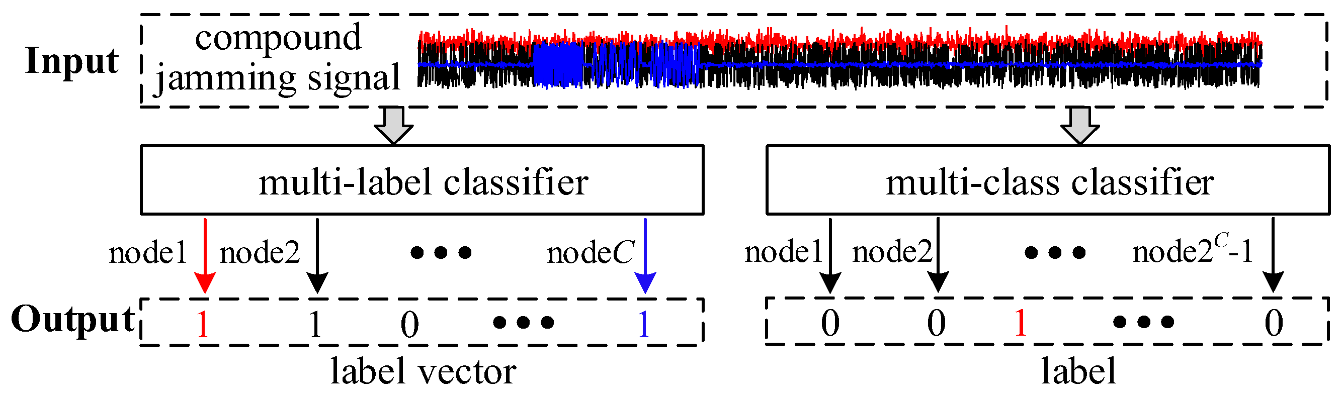
22]. However, these methods cannot deal well with compound signals with strongly overlapping signal components in the time-frequency domain when the suppression jamming power is greater than the power of the other jamming signal components. Some models based on multi-class classification are also used for compound signal recognition [
23,
24]. They define each possible combination as a separate class, which is marked with a single label during the recognition process. A Siamese-CNN model based on the original echo data [
25] and a jamming recognition model based on power spectrum features [
26] realize the recognition of additive and convolutional compound jamming signals, respectively. For the recognition models based on multi-class classification, the size of the output node representing classes increases exponentially with the number of candidate signal components. The feature extractors in models are required to extract the classifiable features of all combinations to ensure recognition performance. Unfortunately, the increasing and overlapping candidate signal components greatly enhance the difficulty of feature extraction, which leads to the increasing model complexity and declining recognition performance.
In addition to multi-class classification methods, another potential strategy that can be used for compound jamming signal recognition is multi-label classification [
27,
28]. It has been successfully applied in many fields such as automatic video annotation [
29], action recognition [
30], visual object recognition [
31], web page categorization [
32], audio annotation [
33], and image recognition [
34,
35]. In terms of radar signal recognition, the multi-instance multi-label learning frameworks based on a CNN and a residual attention-aided U-net generative adversarial network realize the automatic recognition of the overlapping low probability of intercept radar signals [
36,
37]. A CNN-based multi-label framework using time-frequency images is proposed for compound jamming signal recognition [
38]. It has good recognition accuracy at multiple values of the jamming-to-noise ratio (JNR). However, the time-frequency preprocessing comes with an additional computational burden. And the strong overlapping effect of time-frequency images generated by high-power suppression jamming signals is ignored, which can lead to serious degradation of recognition performance when the power of signal components is unbalanced.
Inspired by the multi-label classification methods and considering the problems mentioned above, a multi-label class representation complex-valued convolutional neural network (ML-CR-CV-CNN) with an end-to-end manner is proposed for compound jamming signal recognition. The main contributions of this paper are summarized as follows:
A basic ML-CV-CNN is designed to directly process the raw one-dimensional time–domain compound jamming signals. The introduction of complex-valued components reduces the possible information loss caused by data preprocessing and enhances the weak feature extraction ability for strong overlapping signals.
Using class decoupling implemented by the attention mechanism, the basis ML-CV-CNN is fused with the jamming class representations generated by learning vector quantization (LVQ) to construct the ML-CR-CV-CNN, which enhances the class-related feature learning of compound jamming signals and improves the recognition performance of unseen combinations in training.
Simulation results show that the proposed method can effectively recognize compound jamming signals, especially in the face of high-power suppression jamming signals with strong overlapping effect. The performance improvement is mainly manifested in robustness to the variation of the power ratio (PR), model convergence speed, and generalization to unseen combinations.
The rest of this paper is organized as follows:
Section 2 gives the compound jamming signal model and introduces the basic theory of the recognition model.
Section 3 describes the proposed recognition method in detail. In
Section 4, the data description, experiment configurations, evaluation metrics and experimental results are presented and analyzed. Finally, the conclusions are summarized in
Section 5.
3. Proposed ML-CR-CV-CNN for Compound Jamming Signal Recognition
Considering that radar echo signals are one-dimensional complex data, the basic ML-CV-CNN is designed for the end-to-end recognition of compound jamming signals, where each component in the model is in a complex-valued form. In order to further improve model recognition performance and generalization performance, the ML-CR-CV-CNN is constructed by fusing the jamming class representations into the ML-CV-CNN, which is equipped with a higher ability to learn class-related features required for recognition.
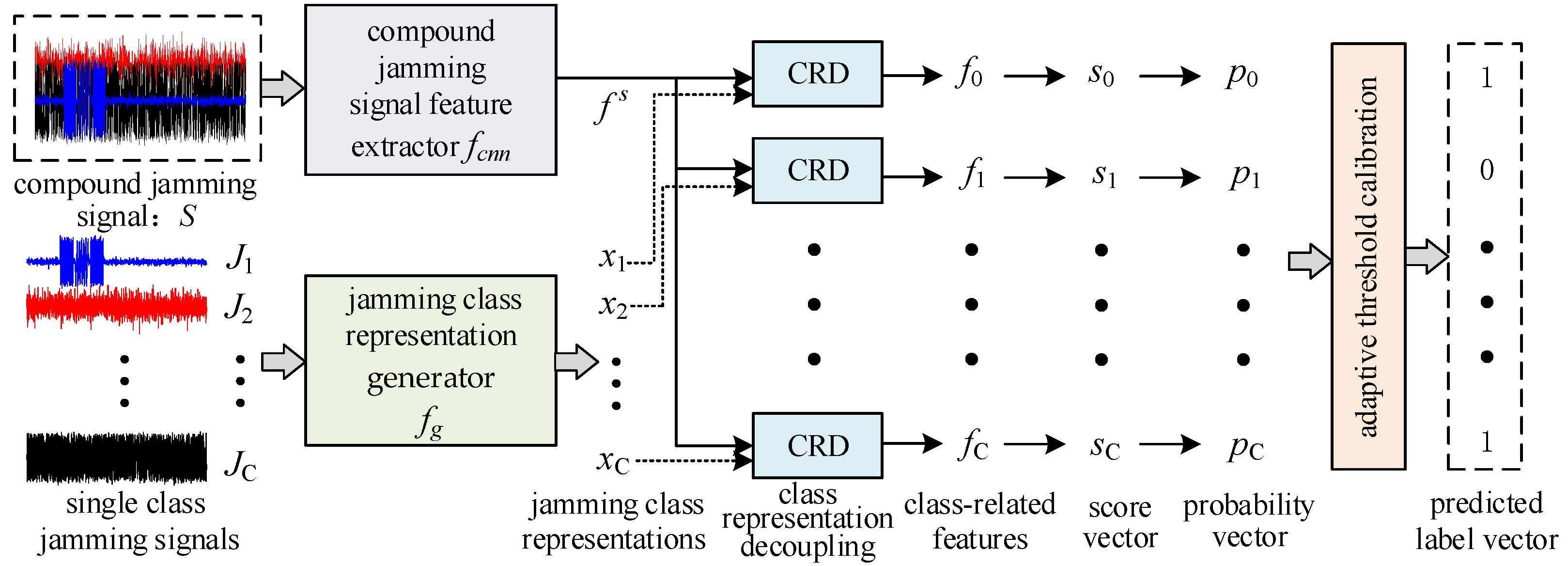
The overall framework of the ML-CR-CV-CNN is shown in
Figure 3. It is mainly composed of four key modules: compound jamming signal feature extraction, jamming class representation generation, jamming class representation decoupling and adaptive threshold calibration. Firstly, for the single jamming signals belonging to different classes, the jamming class representation generator is constructed to obtain the class representations according to a single jamming signal recognition model and prototype clustering. Secondly, through the class representation decoupling module, the features of compound jamming signals extracted by the compound jamming signal feature extractor are fused with class representations to realize class decoupling by the attention mechanism. And then the obtained class-related feature vectors are used to calculate the existence probability of each jamming class. Finally, an adaptive threshold calibration strategy is adopted to select the optimal decision threshold for the probability of each class by maximizing the F1 value. After multi-threshold discrimination, the predicted label vectors can be determined, which are used to recognize the jamming signal components in compound jamming signals. Detailed descriptions of the main modules are given below.
3.1. ML-CV-CNN Model Construction and Compound Jamming Signal Feature Extraction
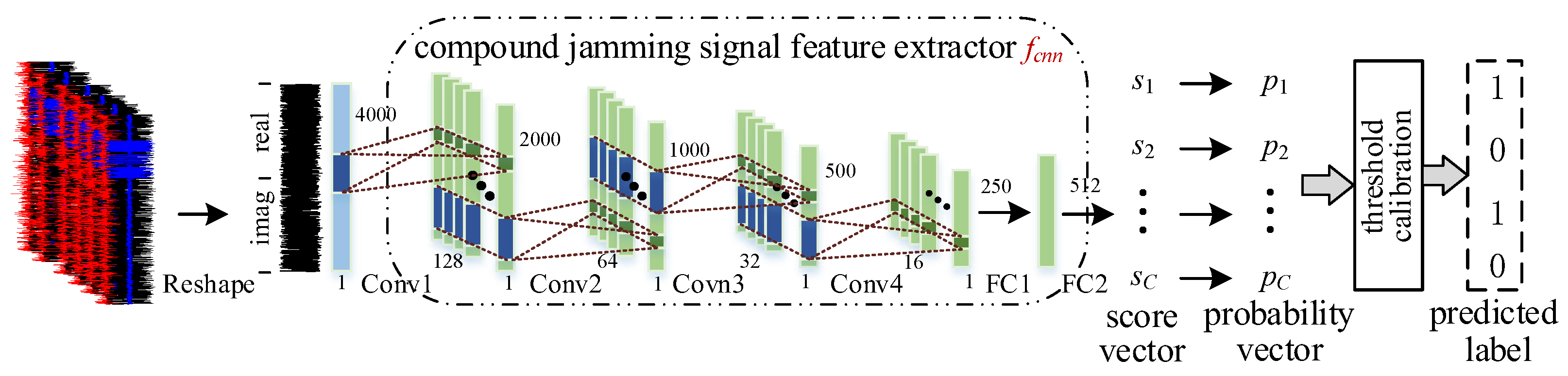
The ML-CR-CV-CNN is constructed by fusing the basic ML-CV-CNN and jamming class representations, where the basic framework of the ML-CV-CNN for compound jamming signals is shown in
Figure 4. The overall structure is an end-to-end recognition model. The input is the one-dimensional time–domain compound jamming signals. After multiple convolutional layers and fully connected layers, the score vectors
representing the confidence level of each jamming class can be obtained. According to
, the probability vectors
indicating the existence of jamming classes can be further calculated by a sigmoid function. And the final predicted label vectors composed of 1 and 0 are estimated to recognize the jamming signal components by performing the adaptive calibration strategy on
.
The specific composition and parameters of each layer in the ML-CV-CNN are shown in
Table 1. Generally, DNNs mainly use real-valued operation. For radar jamming signals, simply separating the real and imaginary parts or considering the amplitude and phase can destroy the original data relationship and lose some information. In order to effectively utilize the phase information and obtain richer signal feature representations for recognition, the layers of convolution, max pooling, activation function and dense in the ML-CV-CNN are implemented by complex-valued operation.
According to the mathematical expression of the complex computation, the complex-valued convolution operation can be expressed as the following [
39,
40]:
where
is a complex vector, which represents the input of the convolutional layer.
is a complex filter matrix, which represents the weight. Among them,
,
,
, and
are all real values.
and
represent the real and imaginary parts of the output of the complex-valued convolutional layer, respectively. It can be inferred that a complex-valued convolutional layer can be realized by a high-dimensional real-valued convolutional layer with two filters. The specific implementation is shown in
Figure 5.
The operation of a complex-valued dense layer is similar to the complex-valued convolutional layer. It can be implemented by a high-dimensional real-valued dense layer with two filters. In addition, a complex-valued activation function and max pooling operation can be achieved by using the rectified linear unit (ReLU) and max pooling (MaxPool) for the real and imaginary data independently. They can be defined as the following [
39]:
where
denotes the complex-valued form.
and
are the real and imaginary parts.
The ML-CR-CV-CNN and ML-CV-CNN share the structure of feature extraction. The compound jamming signal feature extractor
in the ML-CR-CV-CNN can be found in
Figure 4. For the compound jamming signal
that is input into the ML-CR-CV-CNN model shown in
Figure 3, the extracted feature vector
can be indicated as
3.2. Jamming Class Representation Generation
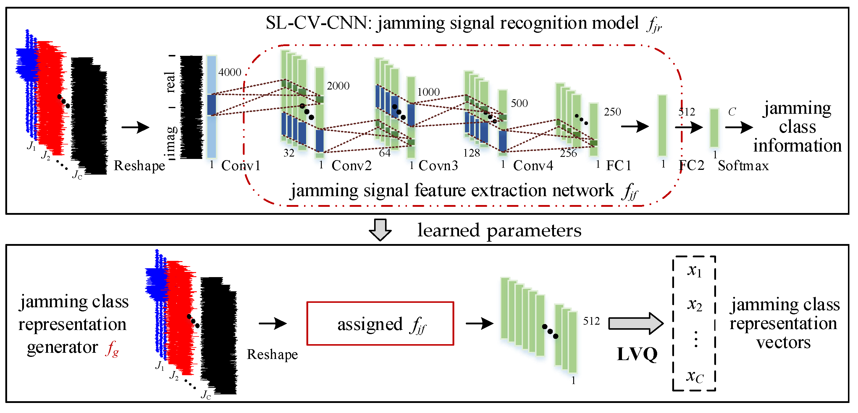
The jamming class representation generator combining a feature extraction network and prototype clustering is utilized to extract the feature vectors that can represent the separability of various types of jamming singles. The feature vectors with sufficient separability are used as jamming class representations, which can help to extract the class-related information from compound jamming signals. Based on the separable feature vectors extracted by a classic end-to-end jamming signal recognition model and the prototype clustering performed by the LVQ algorithm, the jamming class representations can be determined. The specific implementation is shown in
Figure 6.
As shown in
Figure 6, the jamming class representation generator shares the feature extraction network with the recognition model implemented by a single-label complex-valued convolutional neural network (SL-CV-CNN). The composition of the convolutional layer and FC1 layer in the SL-CV-CNN is the same as the ML-CV-CNN, which can be found in
Table 1. And the mapping between the input signal and output label can be formulated as
where
is a single time–domain jamming signal.
is the learnable parameter.
is a single label value indicating jamming classes.
In the process of obtaining jamming class representations, a dataset where each sample is the jamming signal with a single class is first used to train the SL-CV-CNN model. The learned parameters are saved and utilized to assign the jamming signal feature extraction network
. For
single jamming signal samples containing
classes, the sample feature set
can be obtained, where
and
are the feature vector and class label of the
i-th jamming signal sample.
can be denoted as
Then, with the aid of class labels, the LVQ algorithm is used to find the prototype vectors of the obtained feature vectors as the jamming class representations by multiple iterations. Using sample mean vectors to initialize a set of prototype vectors
, one iteration in the LVQ algorithm can be expressed as
where
is the learning rate. After multiple iterations and updates, the obtained prototype vectors are regarded as the final jamming representation vectors
, where
corresponds to the jamming signals
belonging to the class
and has the same dimension as the compound jamming signal feature vector
. Algorithm 1 shows the detailed process of jamming class representation generation.
| Algorithm 1: Jamming class representation generation. |
Require: network model SL-CV-CNN; labeled training samples while not done do select samples with a batch size of ; for do predict jamming signal sample label ; end for compute the cross entropy loss and update the learned parameter ; end while assign the feature extraction network using the learned parameter ; perform prototype clustering on the obtained sample feature set ; initialize prototype vectors ; while not done do randomly select a sample and calculate the distance ; update using Equation (9); end while Output: jamming class representations: final prototype vectors .
|
3.3. Jamming Class Representation Decoupling
The jamming class representation decoupling module mainly uses the jamming class representation vectors to assist the ML-CR-CV-CNN to learn the class-related features required for recognition from compound jamming signals. The class decoupling is realized through the attention mechanism guided by jamming class representations.
After acquiring the jamming class representation vector and , the attention mechanism is adopted to guide to pay more attention to the features related to the class by fusing . The class-related features are learned by the following steps.
The low-rank bilinear pooling method is used to fuse the compound jamming signal feature
and
, which can be formulated as [
34]
where
is the hyperbolic tangent function.
,
,
, and
are the learnable parameters during training.
is the transpose of
. ⊙ represents the element-wise multiplication.
- 2.
The attention weighting coefficient obtained by an attention function can be calculated as follows:
where
is implemented by a fully connected network. The dimension of
is the same as
, and each value
in
represents the importance of the location
in the compound jamming signal feature vector
. The SoftMax function can normalize
to an interval of 0–1, which is defined as
- 3.
The normalized attention coefficient vector is used to perform the weighted average pooling for all locations of , and the obtained feature vector related to the class can be formulated as
By performing the above steps for all types of jamming signals, the class-related feature vectors can be obtained, wherein the related features of the jamming signal components that are present are strengthened, while the related features of the jamming signal components that are not present are weakened.
Based on the obtained class-related feature vectors by the jamming class representation decoupling module, the confidence score vector
for the existence of jamming classes can be predicted by the function
implemented by a fully connected network, where the score
of the class
can be expressed as
Then, the sigmoid function
is adopted to convert the predicted score vector to the probability vector
with values between 0 and 1, where the probability
of the class
can be calculated as
3.4. Adaptive Threshold Calibration
Generally, only the label with the highest probability is selected as the final result for multi-class classification tasks. However, since the ultimate goal of multi-label classification tasks is to determine whether the jamming signal class represented by each value in the probability vector exists, the decision threshold needs to be selected for every probability value . Compared with selecting a fixed threshold for different classes, selecting different thresholds adaptively based on the predicted probability of multiple samples can maximize the performance of the multi-label classifier.
In order to make the classification result not biased towards a high accuracy or a high recall rate, the threshold that maximizes the F1 value can be selected as the final decision threshold
for the class
according to the precision–recall curve. It can be expressed as
where
represent the predicted label and the true label of the class
of the
i-th sample, respectively.
is the sample size.
Depending on the obtained multiple thresholds
, the probability vector
can be converted into a predicted label vector
through a multi-threshold decision function
, where the label
of the class
can be formulated as
4. Experiments and Results
In this section, compound jamming signal recognition experiments are carried out to verify the superiority of the proposed method. The data description, experiment configurations, and evaluation metrics are given. And the results of several groups of comparative experiments are analyzed.
4.1. Data Description
The radar transmitting signal is a linear frequency modulation signal, and the basic signal parameters are shown in
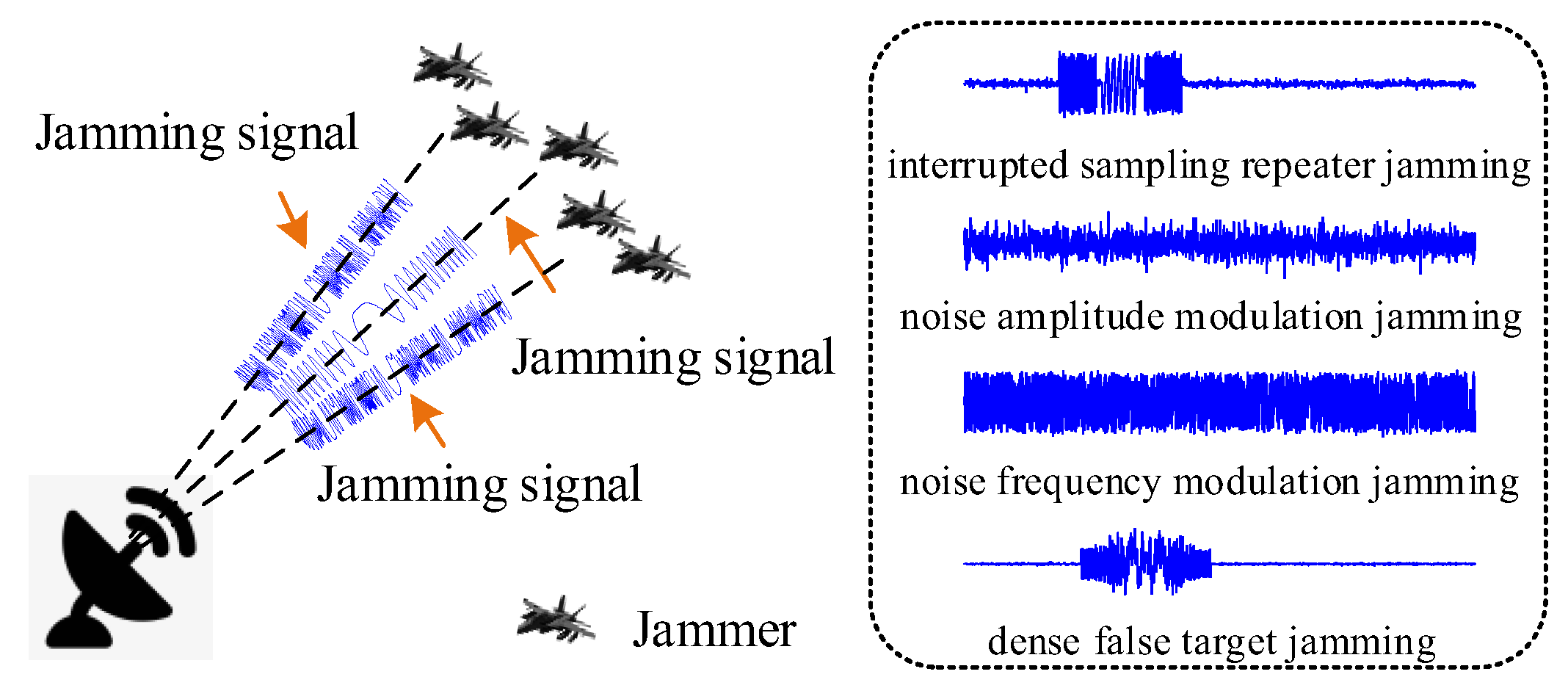
Table 2. The simulated jamming signals are single pulse signals, and the key modulation parameters can be adjusted. In the following simulation experiments, the number of candidate jamming signal components is set to 4. The jamming types cover typical suppression jamming generated by noise modulation and deception jamming generated by the full-pulse repeater and interrupted-sampling repeater, which are interrupted sampling repeater jamming, noise amplitude modulation jamming, noise frequency modulation jamming, and dense false target jamming, respectively [
22,
26]. These four types of jamming are marked as class1-class4 sequentially.
In
Table 2, the JNR of compound jamming signals is defined as
where
denotes the power of the
i-th jamming signal component.
denotes the power of the AWGN.
The PR of different jamming signal components in compound jamming signals is defined as
where
and
represent the power of the
i-th and
j-th jamming signal components, respectively.
Due to the different recognition tasks of the SL-CV-CNN model for single jamming signals and the ML-CR-CV-CNN model for compound jamming signals, two different datasets are required for model training separately.
SL-CV-CNN: Each sample in the dataset contains a single jamming signal class. There are 150 samples for each class and 600 samples in total.
ML-CR-CV-CNN: Since the number of signal components contained in the received compound jamming signals is usually unknown, all possible values should be considered during the training phase. The compound jamming signals are composed of a total of 15 combinations in the case of 4 candidate jamming signal components. Each sample in the dataset contains jamming signal components, and the PR defaults to 0. There are 100 samples for each combination and 1500 samples in total.
4.2. Model Training and Experiment Configurations
For the SL-CV-CNN, the training dataset contains samples , where and are the i-th single jamming signal sample and the corresponding class label. The end-to-end recognition model is trained by the cross entropy loss. And the learned parameters of the jamming signal feature extraction network in the SL-CV-CNN are used to assign the parameters of the jamming class representation generator .
For the ML-CR-CV-CNN, the training dataset contains
samples
, where
is the
i-th compound jamming signal sample and
is the true label vector of the
i-th sample. Each value of 0 or 1 in the vector indicates the absence or presence of the class
. For the samples with a batch size of
, the training objective using the binary cross entropy is expressed as
where
is the probability value of the class
of the
i-th sample, and
is the learnable parameter. The ML-CR-CV-CNN is trained by the Adagrad optimization algorithm with an epoch of 120 and a batch size of 32. The initial learning rate is 0.01, and it drops by 50% after every 30 epochs.
Since the parameters pre-trained on the single jamming signal dataset have a certain generalization ability on the compound jamming signal dataset, the parameters of the jamming class representation generator learned by training the SL-CV-CNN model are utilized to initialize the compound jamming signal feature extractor . In the process of the ML-CR-CV-CNN model training, the parameters of the first three convolutional layers are fixed, and the other layers are jointly optimized.
4.3. Evaluation Metrics
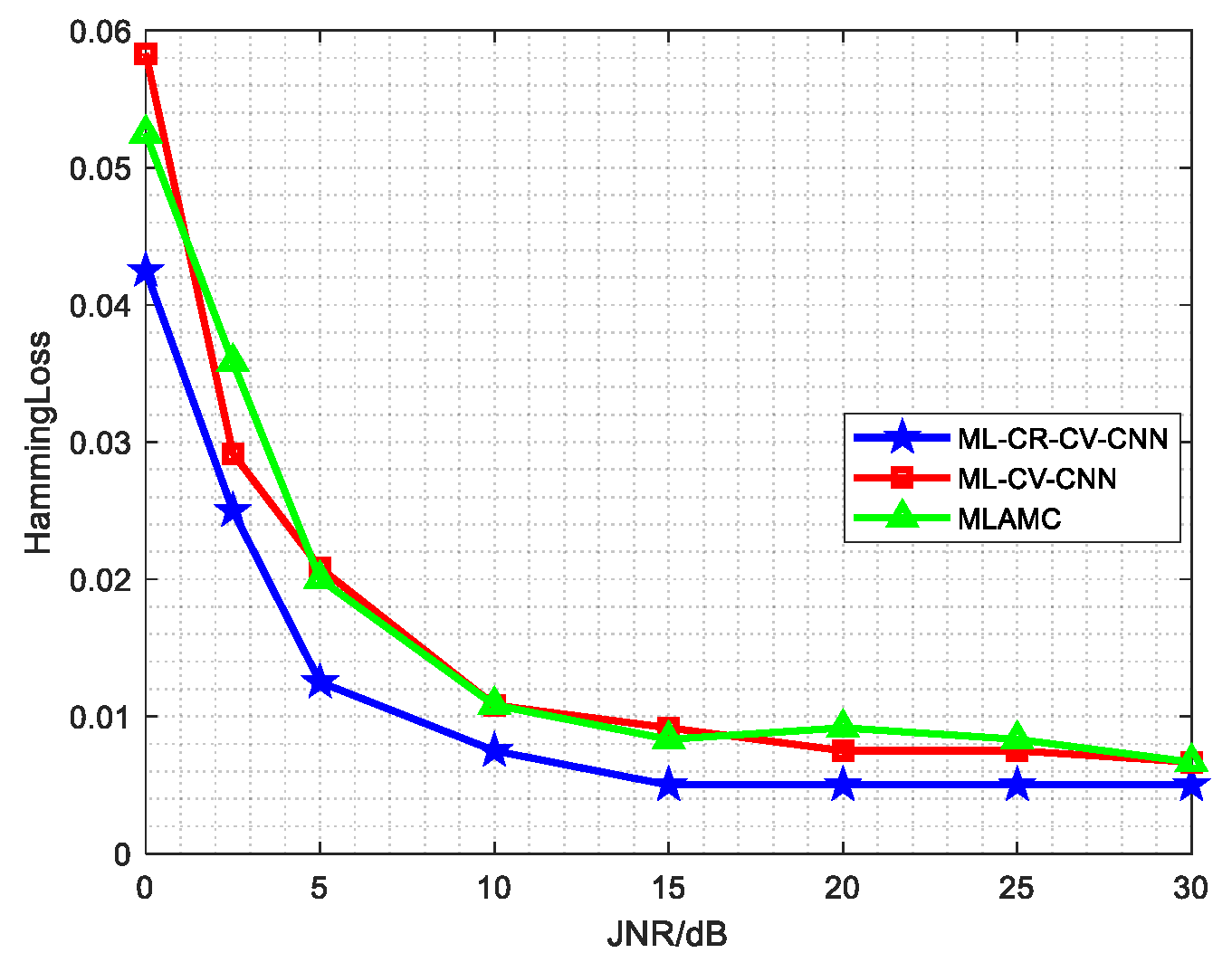
In the compound jamming signal reorganization, the evaluation metrics are calculated based on the predicted label vectors of the ML-CR-CV-CNN. Due to the cases of complete and partial matching between the predicted label vectors and the real label vectors, the subset accuracy and Hamming loss are used to evaluate the overall recognition performance. In addition, the partial accuracy and label accuracy are calculated to evaluate the fine-grained performance.
Each value in the label vector corresponds to the class label of a jamming signal component in compound jamming signals. For the case of complete matching, the subset accuracy (subsetacc) is used to measure the proportion of correctly recognizing all jamming signal components, and the Hamming loss is used to measure the proportion of misclassifying jamming signal components. They can be calculated as follows [
27]:
where
and
denote the predicted label vector and the true label vector of the
i-th sample, respectively.
and
denote the predicted label and the true label of the class
.
represents the number of testing samples. The subsetacc is recorded as 1 when
.
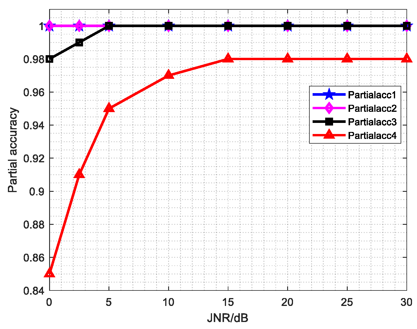
In addition to the complete matching of the predicted results, there are also a large number of cases of partial matching. The partial accuracy (partialacc) and label accuracy (labelacc) can be adopted to evaluate the proportion of correctly recognizing at least
jamming signal components and the proportion of correctly recognizing a certain class of jamming signal components, respectively. They can be calculated as follows [
38]:
4.4. Results and Performance Analysis
The recognition performance of compound jamming signals is affected by many factors such as JNRs, PRs, the number of candidate jamming signal components, and the selection of training samples. Considering these factors, corresponding experiments are carried out to verify the robustness and effectiveness of the proposed method. In this section, the visualization of jamming class representations is first presented. And then the ML-CV-CNN and MLAMC [
38] models based on multi-label classification and the 1D-CNN [
25] model based on multi-class classification are adopted as baseline methods to further demonstrate the advantages of the proposed ML-CR-CV-CNN method in terms of model convergence speed, robustness to varying PRs, and generalization to unseen combinations.
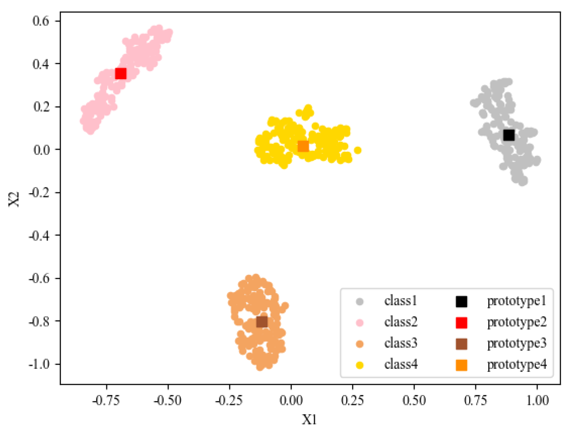
4.4.1. Visualization of Jamming Class Representations
As shown in
Figure 6, the output of the jamming class representation generator is complex feature vectors with a dimension of 256. The real and imaginary data are serially arranged as 512-dimensional real vectors by the reshaping operation. In order to conveniently observe the distribution of high-dimensional feature vectors in the latent space, the tSNE [
41] is used for dimensionality reduction and visualization.
The visualization result is shown in
Figure 7. Observing the feature distribution of single jamming signal samples passing through the jamming signal feature extraction network in the SL-CV-CNN, the feature vectors belonging to different classes of jamming signals form four clusters. The clusters of different classes show clear separability, and the feature vectors in the same cluster show aggregation. As mentioned above, the jamming class representations are generated by finding the prototype vectors belonging to different classes using the LVQ algorithm. As shown in
Figure 7, there are four prototypes corresponding to the four clusters composed of the feature vectors belonging to different classes. And the feature distribution of samples belonging to the same class is concentrated near the corresponding prototype. The prototype vectors with significant separability can be used as the jamming class representations, which can represent the class-related information of different classes of jamming signals. In the ML-CR-CV-CNN, the fusion of jamming class representations is beneficial for extracting the class-related features in compound jamming signals to improve recognition performance.
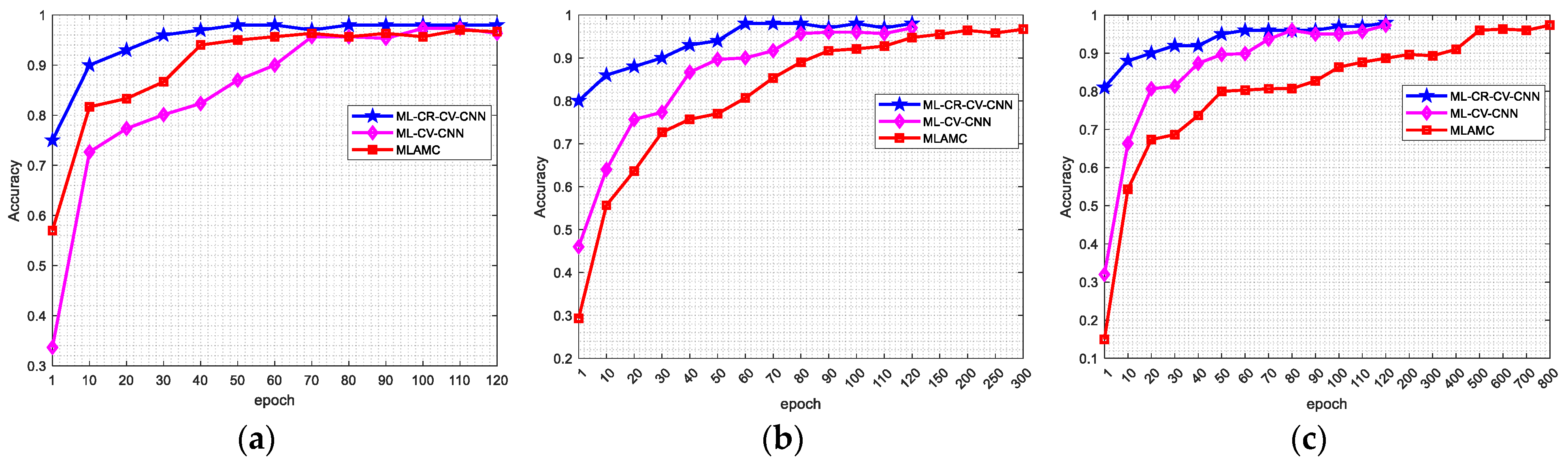
4.4.2. Recognition Model Convergence Speed
In the training process, it is expected to consume the least amount of time to achieve the fast convergence of models. In addition to model structures, the selection of different datasets also affects model convergence speed. In this experiment, the datasets with and JNR = 15 dB, 25 dB, and 30 dB are selected to verify the convergence performance of the three recognition models based on multi-label classification.
Figure 8 shows the subset accuracy of various models with varying epochs under different JNRs. As shown in
Figure 8a, all three models can reach convergence after 70 epochs at JNR = 15 dB. Further observing the results with JNR = 25 dB and JNR = 30 dB shown in
Figure 8b,c, it can be seen that the convergence speed of the ML-CV-CNN and ML-CR-CV-CNN models is stable and similar to that of JNR = 15 dB. However, the MLAMC model is more sensitive to varying JNRs. And the convergence speed decreases with increasing JNRs. At JNR = 25 dB and JNR = 30 dB, it needs about 150 and 500 epochs to achieve convergence, which takes longer than the other two models. Therefore, it can be inferred that it is more difficult for the MLAMC model to extract the time-frequency features of different jamming signal components for recognition when suppression jamming signals with high JNRs generate stronger overlap on time-frequency images. In contrast to the MLAMC model, the ML-CV-CNN and ML-CR-CV-CNN models using one-dimensional complex-valued operation are more conducive to extracting the weak features of compound jamming signals at high JNRs, and the model convergence speed is faster and more independent of the influence of JNRs. In addition, benefiting from the jamming class representation fusion, the ML-CR-CV-CNN model takes less time to achieve the same accuracy and model convergence compared with the ML-CV-CNN model.
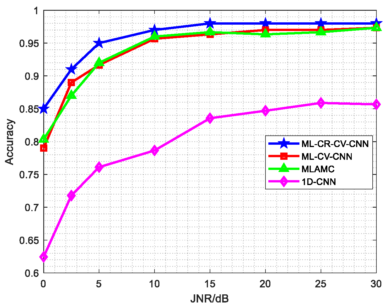
4.4.3. Recognition Performance Versus Number of Candidate Jamming Signal Components
When the number of candidate jamming signal components is 1, the compound jamming signal recognition is equivalent to the single jamming signal recognition, which usually has good performance. When the value of is large, the compound jamming signals with complex components and multiple combinations can lead to a certain degree of degradation in recognition performance. In this experiment, three datasets with varying values of are used to evaluate the robustness of the proposed method to the varying numbers of candidate jamming signal components. The corresponding specific components are class1-class2, class1-class3, and class1-class4.
Table 3 shows the subset accuracy with varying values of
for various recognition models under multiple JNRs. It can be observed that the recognition accuracy decreases with the increasing values of
. Compared with the other baseline methods, the proposed ML-CR-CV-CNN model has the slightest performance degradation at
and exhibits optimal results, especially at low JNRs. At JNR = 5 dB and 25 dB, the accuracy improves by 3% and 1% compared to the suboptimal results, respectively. In addition, the three models based on multi-label classification are significantly better than the 1D-CNN model in terms of recognition accuracy and robustness to varying JNRs and values of
. The results demonstrate the absolute superiority of the recognition models based on multi-label classification in the problem of compound jamming signal recognition with a large number of candidate jamming signal components.
4.4.5. Recognition Performance Versus PRs
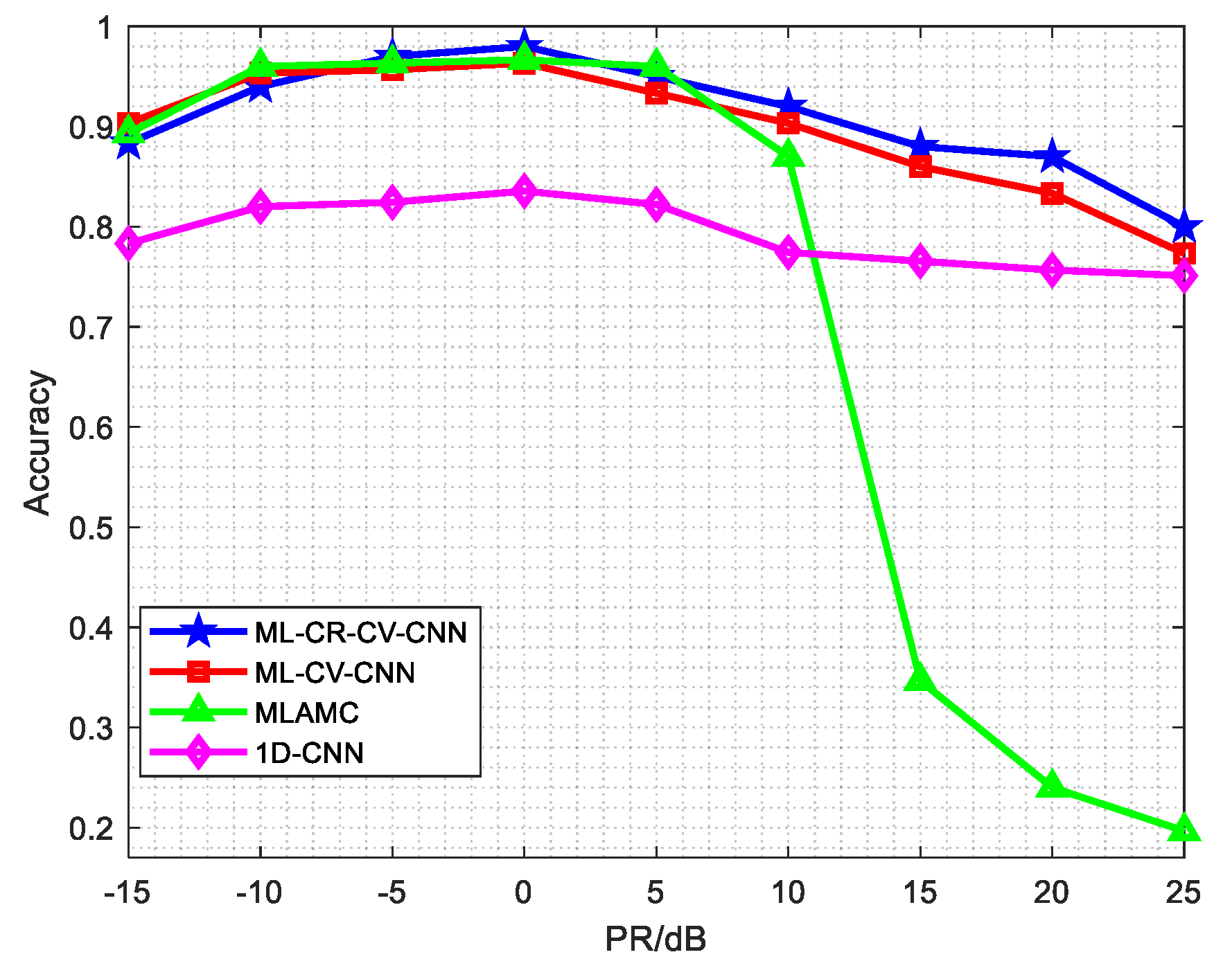
All the above experiments are carried out under the setting of PR = 0 dB. The power of each component in compound jamming signals is equal. Usually, in order to effectively achieve the jamming effect, the power of suppression jamming signals is higher than the deception jamming signals according to the generation mechanism. Therefore, considering the different energy losses caused by unequal propagation distances and transmitting power of different jammers, the intensities of the jamming signal components in compound jamming signals received by the radar are usually unequal. And the power imbalance causes fluctuations in recognition performance. In this experiment, the influence of different PRs on the overall recognition performance is verified by changing the power of one jamming signal component. The JNR is fixed at 15 dB, and the power of the noise frequency modulation jamming signal is adjusted.
Figure 12 shows the subset accuracy with varying PRs for various recognition models. It can be seen that the three models based on multi-label classification can obtain better performance at multiple PRs compared with the 1D-CNN model. The accuracy of the ML-CV-CNN and ML-CR-CV-CNN models is more robust to the variation of PRs than that of the MLAMC model. When the power of each component in compound jamming signals is equal (PR = 0 dB), the subset accuracy reaches the maximum. Using the result at PR = 0 dB as the baseline, the accuracy decreases to varying degrees with decreasing or increasing PRs. At PR > 0 dB, the degree of decline is much greater than the results at PR < 0 dB. Especially for the MLAMC model, the accuracy declines rapidly at PR > 10 dB due to the strong coverage effect on time-frequency images caused by high-power suppression jamming signals. In contrast, the ML-CV-CNN and ML-CR-CV-CNN models using one-dimensional complex data show stronger ability in mining strong overlapping signal features when the high-power suppression jamming signal exists, and the accuracy is effectively improved at PR > 10 dB. In addition, benefiting from the fusion of jamming class representations, the performance of the ML-CR-CV-CNN model is slighter better than that of the ML-CV-CNN model at PR > 0 dB, and the decline caused by the strong overlapping effect of high-power suppression jamming signals is further alleviated. At PR = 15 dB, the accuracy of the ML-CR-CV-CNN model is close to 88%, which is 52% higher than the MLAMC model.
4.4.6. Recognition Performance of Unseen Jamming Signal Combinations in Training
In the presence of many candidate jamming signal components, the size of the compound jamming signal dataset containing all possible combinations is large. In order to reduce the difficulty of sample acquisition and improve the training speed, it is expected that only partial samples in the dataset are used to train recognition models, and good recognition results can be achieved for all combinations simultaneously. For the jamming signal combinations that do not appear in training, the correct recognition of jamming signal components requires that the recognition models have some generalization and extensibility. In this experiment, three training sets containing partial combinations are used to evaluate the recognition performance of the trained models against unseen jamming signal combinations. For the three datasets, the JNR and PR are fixed at 15 dB and 0 dB, and the compositions of jamming signal components are , , and . Thus, the corresponding unseen jamming signal combinations to be tested consist of , , and .
The 1D-CNN model based on multi-class classification does not have the ability to recognize jamming signal combinations that have not been seen in training.
Figure 13 shows the subset accuracy of unseen jamming signal combinations when the ML-CR-CV-CNN, ML-CV-CNN, and MLAMC models use partial combinations for model training. The black dashed line represents the average subset accuracy for all unseen combinations containing different possible values of
. It can be observed that the recognition performance of the three models has a similar trend with various training sets. With the enrichment of jamming signal combinations in training sets, the accuracy of unseen combinations increases. When the training set consists of only single jamming signals (
), the ML-CR-CV-CNN model has the best recognition result by comparing the three models horizontally. Especially for the test samples with
and
, the accuracy is significantly higher than that of the ML-CV-CNN and MLAMC models. In this case, only 26.7% of jamming signal combinations participate in model training for the dataset containing all possible jamming signal combinations. The ML-CR-CV-CNN model still has an average subset accuracy of 74.36% for the testing samples that have not been seen in training, which is 21% higher than the ML-CV-CNN model and 27% higher than the MLAMC model. The results demonstrate that the fusion of jamming class representations in the ML-CR-CV-CNN greatly enhances the generalization and extensibility for unseen jamming signal combinations.


