1. Introduction
A radar emitter is the core component of a radar system. It produces a radio frequency (RF) signal with sufficient power and transmits it through an antenna. To avoid being intercepted by electronic reconnaissance equipment, hostile radar emitter structures (RES) have become increasingly diverse. In this paper, the RES can contain many different radar emitter individuals (REI), and they are considered as a class of structures. Thus, in complex electronic reconnaissance situations, the hostile radar cannot be deeply recognized, through only the radar modulation type identification [
1,
2] and REI identification [
3,
4,
5,
6,
7,
8,
9,
10,
11]. Therefore, this paper studies methods for inverting RES from RF signals emitted by radar emitters to provide more information at a new level on electronic reconnaissance systems. There are essential differences between REI identification and RES inversion. REI identification is the identification of differences between individuals in different radar emitters, while RES inversion focuses on the differences in radar emitter structures. Thus, REI identification and RES inversion are studies of radar emitters at different levels, and they have essential differences. At this moment, we are only interested in RES and not REI. Simultaneously, if the same class of RES contains different REIs, it will introduce certain challenges to RES inversion.
The non-ideal characteristics generated by each REI as “RF individual information” and the overall non-ideal characteristics generated by each class of RES are called “RF structure information” in this paper. In addition, each class of RES has unique inherent characteristics. Different classes of RES have different physical mechanisms and different RF structure information. At the same time, the radar-emitted RF signal will carry these unique RF structure features; therefore, RES inversion can be achieved using RF structure features.
Meanwhile, with the emergence of multifunctional radars, radar-emitted RF signals are becoming increasingly complex. Signals with different modulation types and operating parameters are used when performing different tasks. Therefore, different operating parameters can cause signal differences between RF signals, which are called “signal information” in this paper. Therefore, RF signals are mainly influenced by two factors: signal information and RF information. The complex situation is that the parameters’ change randomly introduces great challenges to the electronic reconnaissance system.
The performance of RES inversion depends on the stability and separability of extracted features. At present, feature extraction methods are mainly divided into the time domain [
12], frequency domain [
13], time–frequency domain [
14], and transform domain [
15,
16,
17,
18,
19,
20,
21]. The shortcoming of these methods is their reliance on professional knowledge and experience for manual feature extraction and design. In recent years, deep learning technology [
22,
23] has been widely used in various fields, including speech [
24] and image [
25] processing. It has also been widely used in radar emitter identification fields [
26,
27,
28,
29,
30,
31], integrating artificial intelligence technology with radar identification. Specially in the study of REI identification [
26,
29,
32], in general, various neural networks can effectively carry out corresponding tasks under the condition of having good training data and corresponding labels (i.e., closed-set problem). Meanwhile, as an unsupervised network, the autoencoder (AE) [
33] has been proven to have excellent performance in feature representation. Different improvements have been made for different situations, such as sparse autoencoders (SAE) [
34,
35,
36], stacked sparse autoencoders (sSAE) [
37,
38], denoising autoencoders (DAE) [
39,
40], and compression autoencoders (CAE) [
41]. However, unsupervised learning does not always produce the desired results in the case of unknown operating parameters (i.e., open set problem). If labels are used to enhance the separability of features, combining supervised and unsupervised training can improve the performance of the neural network.
However, whether using traditional feature extraction methods or neural networks, these methods mainly focus on the homo-mode operating parameters (constant operating parameters), in which conditions are too ideal. What needs to be further discussed is whether these methods have good generalization performance under the hetero-mode operating parameters (variable operating parameters). Thus, the main problem of these methods involves the extraction of the RF features of the RF signal directly. However, these methods do not pay attention to the interference introduced by signal information. Does the extracted RF feature contain a large amount of signal information?
Therefore, the problem to be solved in this paper is as follows: how can we reduce the interference of signal information in complex situations so that the extracted RF structure features have good stability and separability? Moreover, how can these RF structure features be used to achieve RES inversion while retaining the RES inversion algorithm’s good robustness and generalization performance under unknown operating parameters? As far as we know, there are no relevant papers that have examined this issue. It is worth noting that this complexity includes the complexity of RES modeling (we invert the twelve radar emitters into three classes of structures) and the complexity of the variable operating parameters (modulation type, frequency, bandwidth, and input power).
In summary, it is challenging to realize RES inversion in complex situations, and the traditional method can easily fail due the to interference of signal information due to the lack of influence of signal information under variable parameters on extraction of RF features. In the field of radar signal recognition, the closed-set problem of signal modulation type recognition refers to the recognition of known modulation type signals, while the open-set problem refers to the recognition of unknown modulation type signals [
42], and its open-set problem is more challenging. Researchers have introduced metric learning into signal modulation type recognition and demonstrated the advantages of triplet loss functions in feature extraction [
28]. This paper conducts an RES inversion study on closed-set (known operating parameters) and open-set (unknown operating parameters) problems using hetero-mode operating parameters, which combines metric learning and deep learning techniques to study how effectively to reduce the interference caused by signal information. We attempt to find methods that can render the neural network more attentive toward the common RF structure information of RF signals among these hetero-mode operating parameters in the learning process; we also attempt to render the neural network insensitive to changes in terms of operating parameters, and we provide good stability and separability for extracted RF structure features, which is the key to RES inversion.
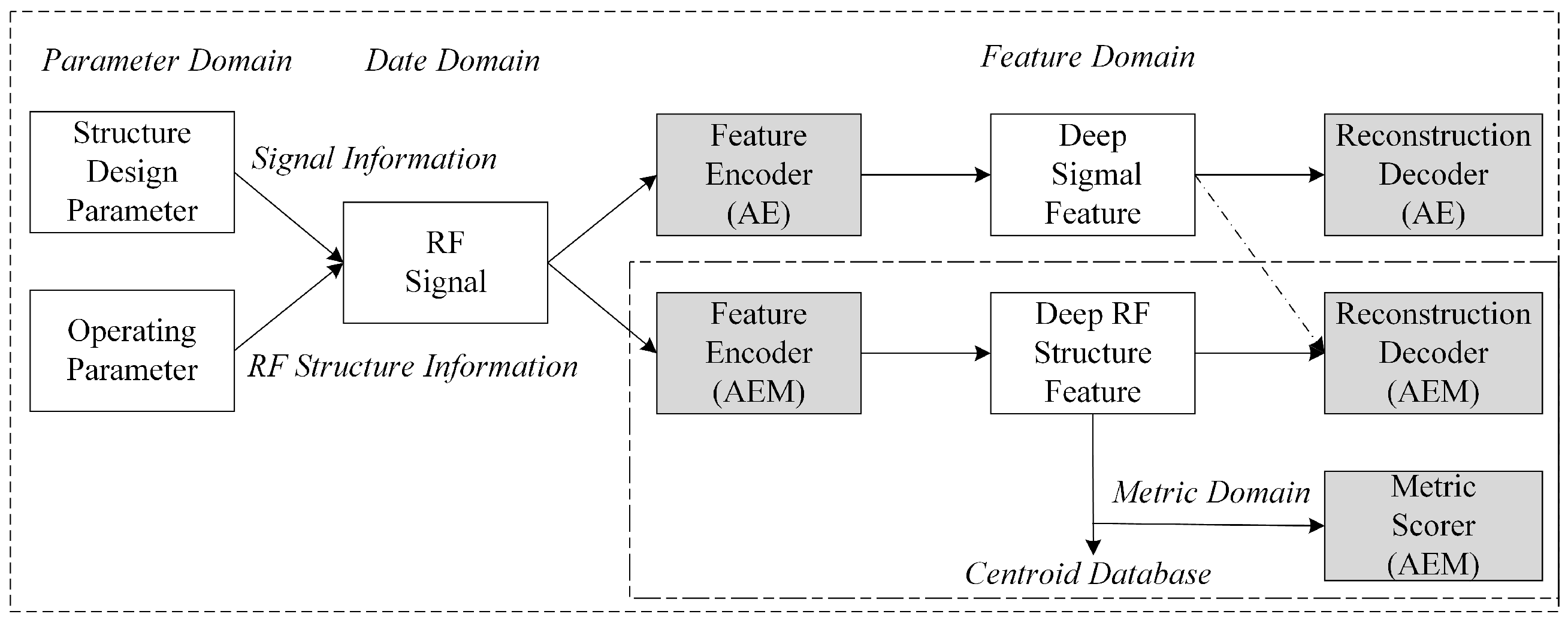
Figure 1 shows the overall flowchart of the method proposed. First, RF signals are obtained using RES modeling. Then, the AEM network is constrained in the feature domain using the deep signal features extracted from the AE network in the data domain, and the RF signal is reconstructed as unsupervised to weaken the signal information in the feature domain of the RF signal under hetero-mode operating parameters; RF structure information is highlighted. Distinct from traditional algorithms, the RF structure features automatically extracted via deep learning are called “deep RF structure features”, and the signal features are called “deep signal features” in this paper.
The main contributions of this paper are summarized as follows:
Stability: A dual neural network (AE and AEM network) is designed based on the idea of unsupervised learning. The use of deep learning techniques to reduce the interference caused by signal information is essential for extracting RF features that are not sensitive to parameter variations. This idea is instructive for RF feature extraction techniques under variable operating parameters.
Separability: Based on the idea of supervised learning, a metric scorer is designed in the AEM network using the metric learning approach; using this, the network shortens the distance of RF signals in the feature domain between the hetero-mode operating parameters of the same class of RES during the learning process, while widening the distance between RF signals in different classes of RES to improve the separability of the deep RF structure features learned from RF signals.
Unsupervised and supervised joint optimization methods are designed to optimize the objective function of AEM networks.
Different from the traditional REI method used with constant operating parameters, the RES inversion method using variable operating parameters (modulation type, frequency, bandwidth, and input power) is proposed for the first time, and centroid-matching method is used for RES inversion from radar-transmitted RF signals in the test stage. Moreover, the proposed method maintains good generalization performance under unknown operating parameters.
The remainder of this paper is organized as follows.
Section 2 introduces the problem’s definition.
Section 3 presents and verifies RES modeling.
Section 4 presents the proposed RES inversion method.
Section 5 details the experimental results and analysis of the proposed method. Finally, the conclusions are drawn in
Section 6.
2. Problem Definition
A radar emitter is the core component of a radar system. Radar emitters are typically classified as pulse-modulated emitters and continuous wave emitters. Pulse-modulated emitters are usually categorized into single-stage oscillating emitters and main vibration amplification emitters. Most radars, particularly those that are highly stable and those with high-performance tracking, telemetry, and control (TT&C), as well as phased array radars, have adopted a main vibration amplification radar emitter. Recently, with the rapid development of gallium arsenide (GaAs) and gallium nitride (GaN), studies on all-solid-state radar emitters in the C-band and X-band have approached the practical stage. All all-solid-state radar emitters are generally classified into two categories: a high-power solid-state emitter with a centralized synthesis output structure and a distributed synthetic phased radar emitter. Therefore, there is a variety of RES due to these different structure design parameters.
Generally, the radar emitter source is mainly composed of a signal source and an RF link module [
43,
44]. The signal source generates a source signal of the desired frequency. The RF mixer and RF amplifier are the core modules of the RF link. The RF mixer is responsible for moving the intermediate frequency signal spectrum to the RF area, and the RF amplifier is responsible for amplifying the input RF signal. Due to the defects of the underlying physical components, the signal source has phase truncation errors, which makes RF signals appear as “burrs” (spurious information). RF modules, such as RF mixers and RF amplifiers, have nonlinear distortion and phase noise, which will produce high harmonics and intermodulation distortion. The phase noise level of the RF mixer can introduce significant differences to the RF signal in both time and time–frequency domains. The different third-order intercept points (IP3) of the RF amplifier will cause different amplitudes in the RF signal.
Because different classes of RES are composed of different structure design parameters, such as RES1 having only one stage of amplification while RES2 is designed for two-stage amplification, there are structure differences between different classes of RES. At the same time, under the same class of RES, different individuals have the same structure design parameters and use the same components, but because there are subtle differences between each component; this subtle difference is called “RF individual information” in this paper, and it is also called an “RF fingerprint” [
45]. This results in individual differences among different individuals under the same RES. Therefore, there are essential differences between REI identification and RES inversion in this paper.
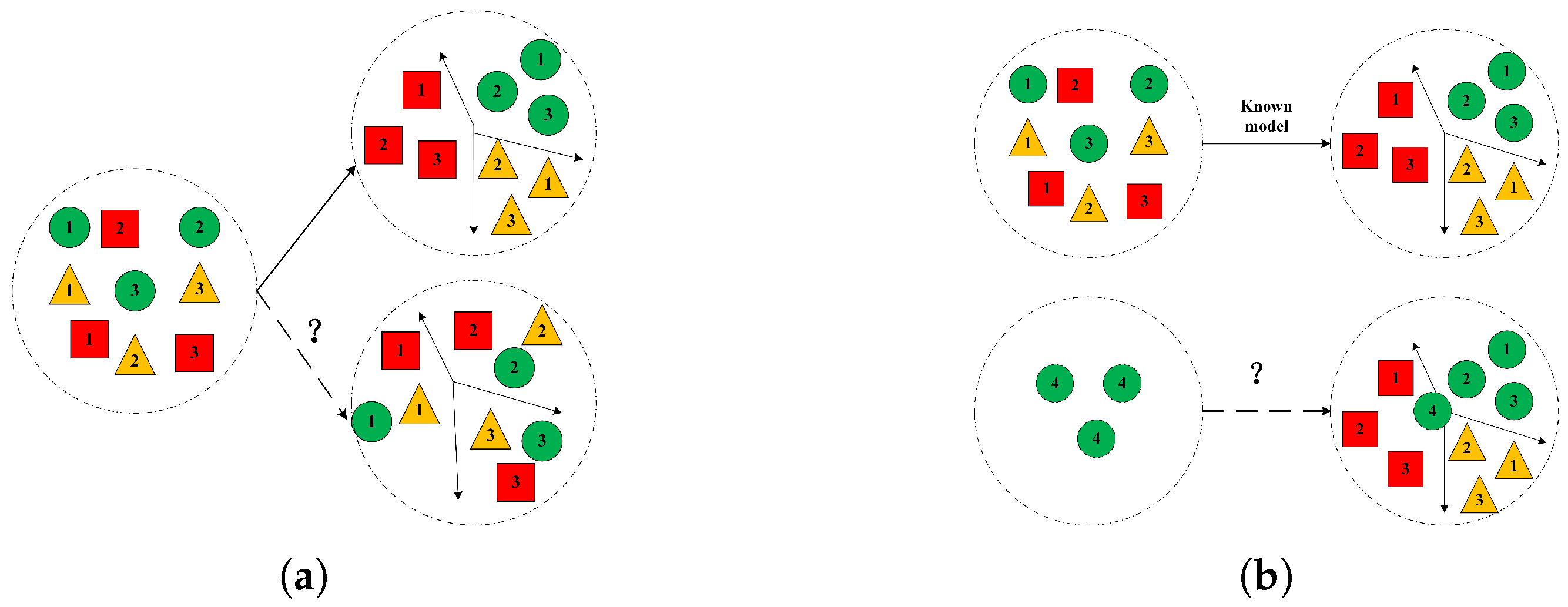
As shown in
Figure 2, red, yellow, and green represent three classes of RES, and numbers 1, 2, and 3 correspond to three different operating parameters, while the number 4 corresponds to unknown operating parameters. The RF structure information carried by RF signals and transmitted by radar emitters with different structures is noticeably different under ideal conditions. All types of neural networks can be used for classification and recognition if using the homo-mode operating parameter—that is, 1, 2, and 3 are the same operating parameters—and the training data and corresponding labels are good.
With the emergence of multi-functional and phased array radars, operating parameters in relation to different tasks can be changed. For instance, multi-functional radars support various modes, such as tracking and searching, single-target tracking, multi-target tracking, and others. The performance of the neural network will be seriously affected either by RES inversion or by REI identification under hetero-mode operating parameters. Next, the influence of the change in operating parameters upon RES inversion is analyzed.
Question 1: Training data question: Although a large amount of training data can be obtained under certain known operating parameters (e.g., the frequency is 25 MHz and 26 MHz), it is not possible to collect all training data within all changing ranges of operating parameters (e.g., the frequency is 27 MHz). Additionally, samples with different operating parameters are often imbalanced (for example, there are more samples at 25 MHz than at 26 MHz) due to the limitations of the working scene, parameter selection and data collection conditions, and other factors. Therefore, a complete database cannot be easily established using electronic reconnaissance systems.
Question 2: The influence of hetero-mode operating parameters: With the improvement in the circuit integration process, the difference in nonlinear characteristics between components is decreasing, but radar operating parameters are constantly changing, and the difference gradually increases. As a result, if the same class of RES transmits RF signals with different operating parameters, the signal information carried by the RES may cover the RF structure information, or it may completely exceed the RF structure information. If different classes of RES transmit RF signals with different operating parameters, the signal information carried by the different classes of RES may exceed the RF structure information that is carried. As a result, the neural network might pay more attention to each signal information, which results in the performance of the neural network being significantly affected by the change in operating parameters. When there are different REIs under the same class of RES, difficulties in classification greatly increases under hetero-mode operating parameters.
Question 3: The influence of unknown operating parameters: When receiving an RF signal with unknown operating parameters transmitted by a known RES, the neural network maps the training data domain to the feature domain completely according to the known operating parameters and determines the classification boundary. When the operating parameters of the received RF signal are not within the operating parameters range of the training data, can this neural network be used to map the RF signal with unknown operating parameters to the feature domain of known operating parameters? Will the neural network make false judgments?
Question 4: The influence of noise: When noise levels are high in the real environment, both the RF signal and structure information may be covered at the same time. It is unknown whether noise will cause the neural network to be unable to extract meaningful features, thereby making the performance of the neural network more sensitive to noise and less robust.
Therefore, the problem to be solved in this paper is to extract the good stability and separability of features that represent RF structure information under this hetero-mode operating parameter; then, this feature is used to invert the RES and make the neural network insensitive to changes in the operating parameters.
3. RES Modeling
The importance of RES modeling lies in the construction of a dataset that corresponds to the actual situation and the generation of the required RF signal using the structure feature level modeling method. This is a forward modeling process that provides a basis for subsequent inversion methods. Having a high-quality dataset is the premise and basis for training neural networks. However, due to the confidentiality of military systems, it is very difficult to obtain RF signals under such hetero-mode operating parameters. Therefore, simulation data [
46,
47] are mostly used to conduct experiments on electronic reconnaissance systems. Hence, RES modeling is the premise of obtaining a simulation dataset, which is of great importance. Large amounts of data can be obtained via the modeled RES.
The current methods for constructing simulation data are mainly classified into two categories: single-device modeling and mathematical modeling. In single-device modeling, power amplifiers are mostly studied [
48,
49,
50,
51], and behavioral modeling, like Saleh [
49], polynomial [
50], and Volterra series [
51] models, is usually used to simulate nonlinear features and memory effect. In mathematical modeling, there are mainly two types of models: a time-domain envelope model that can reflect the transient and steady-state features of the radar emitter [
52], and the phase noise model [
53] with the frequency shift mode [
54] relative to frequency stability that can reflect the spectrum purity of the radar-emitted signal. Their main shortcomings are that they can only reflect the features of a certain module in the RES model but cannot fully reflect its overall features.
Therefore, to provide basic conditions for theoretical analyses and the practical verification of this study, this paper builds three classes of RES models by selecting different structure design parameters and using a simulation platform with measured parameters according to the working principle of radars. The S2P file is used for simulation, and the S2P file can be approximately considered as the reflection of a field measurement component in software. Therefore, the simulation data are closer to real data. In addition, under the same RES model, four REI models are built by slightly adjusting the parameters of each module. As a result, there are structural differences among the RES models of different classes and individual differences among different REI models of the same class when building RES in complex situations.
3.1. RES Model
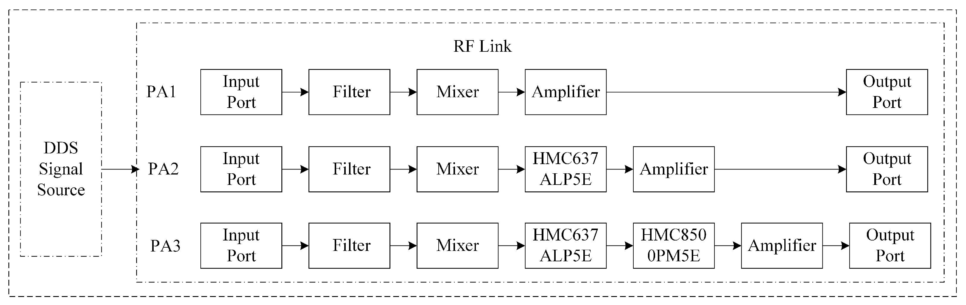
As shown in
Figure 3, a signal source model and three RF link models (PA1, PA2, and PA3 models) are built. Three RES models (RES1, RES2, and RES3) of different classes are developed by combining the signal source and RF link models. Each RES model includes two parts, the signal source model and RF link model, which are introduced in detail in the following sections.
3.1.1. Signal Source Model
Considering that direct digital synthesizer (DDS) technology has become the mainstream of signal sources in modern radar emitters, in the actual circuit, the DDS model increases the number of phase accumulator bits in order to improve frequency resolutions. In order to reduce the ROM’s storage capacity, the higher
A bits of the
N bits are selected to address the amplitude information in the ROM, and the
bits are truncated, which introduces a phase truncation error [
55].
Therefore, the DDS model [
55], widely used in the radar application field, was selected as the signal source to generate continuous wave (CW), linear frequency modulation (LFM), binary phase shift keying (BPSK), and quadrature phase shift keying (QPSK) signals using spurious information from the four DDS models of different modulation types, which were built according to the principle of phase truncation error: DDS_LFM model, DDS_BPSK model, and DDS_QPSK model.
DDS_CW model: According to the CW signal simulation principle, the frequency of the DDS_CW signal generated by the DDS_CW model is as follows:
where
N represents the bits number of the phase accumulator,
denotes the frequency of the reference clock source, and
is the frequency control word.
DDS_ LFM model: According to the LFM signal modulation principle, the DDS_LFM model is developed to generate the DDS_LFM signal. To perform the function of linear frequency modulation, the result of the frequency accumulator exhibits a linearly increasing characteristic, while the result of the phase accumulator exhibits the characteristic of a quadratic function. The initial frequency
and bandwidth
of the DDS_LFM signal are expressed as follows:
where
represents the frequency control word,
denotes the chirp rate control word (i.e., frequency step word), and
T denotes the pulse width.
DDS_BPSK model: The DDS_BPSK model is developed according to the BPSK signal modulation principle. The DDS_CW signal is used as a carrier signal, and the DDS_BPSK signal is generated using a 7-bit Barker code .
DDS_QPSK model: The DDS_QPSK model is developed according to the QPSK signal modulation principle. The DDS_CW signal is used as a carrier signal, and the DDS_QPSK signal is generated using the phase encoding .
3.1.2. RF Link Model
Practically, the signal generated by the signal source should undergo multi-stage amplification to achieve the transmission power required for the transmission distance. The parameter simulation of each component is performed using the S2P file. The latter is composed of the S parameter () matrix, and the value of the S parameter is obtained by the manufacturer’s field measurement of the component. Therefore, an S2P file can be approximately considered as the reflection of a field measurement component in the software.
The RF link model is built using different amplification stages and module parameters. The RF mixer module is set as a linear device, and the RF amplifier module is set as a nonlinear device, which includes the following: the PA1 model is a first-stage amplifier, which uses the simulation amplifier; the PA2 model is a two-stage amplifier, which uses the HMC637ALP5E GaAs power amplifier and simulation amplifier; and the PA3 model is a three-stage amplifier, which uses the HMC637ALP5E GaAs power amplifier, the HMC8500PM5E GaN power amplifier, and the simulation amplifier.
The individual differences of each class of RES models are simulated by slightly adjusting the phase noise level and frequency offset of the RF mixer and the IP3 value of the RF amplifier. The specific parameters of each module are shown in
Table 1. The reference impedance is 50 ohms, the noise figure is 8 dB, and the operating frequency of these devices is 2.1 GHz.
3.2. RF Signal
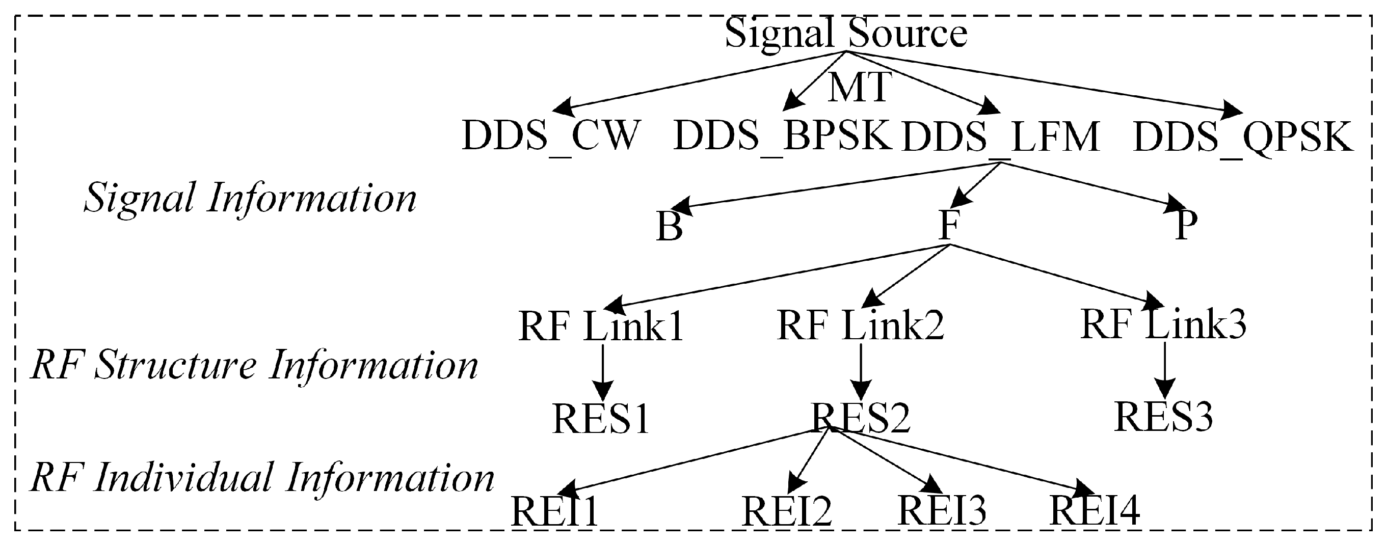
Based on the above modeling, different operating parameters, namely, the modulation type (MT), frequency (F), bandwidth (B), and input power (P), are selected to generate source signals with four DDS signal source models, and complex signals are obtained using Hilbert transformations as input signals to the RF link model. They are then amplified by PA1, PA2, and PA3 models and output as RF signals of three classes of RES models.
As a result, RF signals generated by modeling are composed of different structure design parameters and different operating parameters. Different operating parameters cause differences in signal information between RF signals, and different structure design parameters cause differences in RF structure information between RF signals, as shown in
Figure 4. The modeling dataset for complex situations is generated. This includes three classes of RES models and four REI models under the same class of RES model, i.e., a total of twelve radar emitters.
4. RES Inversion Method
As observed in the above modeling, different structure design parameters and operating parameters can produce various RF signals that carry different RF structure information and signal information, or they map the parameter domain to the data domain. If the data domain can be mapped to the feature domain so that the neural network can learn the relevant features representing the RF structure information and signal information, it will be conducive to the RES inversion.
Then, by comparing the channel system [
56], the RES can be regarded as an RF structure system,
, which carries RF structure information. Different classes of RES correspond to different RF structure systems because they are composed of different structure design parameters and carry different RF structure information. This is a complex nonlinear and unknown system; the specific parameters of the system cannot be obtained via simple calculations.
The ideal RF signal
without RF structure information, that is,
, can be considered as the baseband signal
with different operating parameters after passing through the modulation system
:
Therefore, the RF signal
carrying RF structure information can be considered as the ideal RF signal obtained via the RF structure system:
Based on the above analysis, a dual neural network is designed in this section. An AE network aims to train a feature encoder that is capable of extracting deep signal features in an unsupervised manner using ideal RF signals. As for the AEM network, the feature encoder of the AE network is used to extract the deep signal features, constrain the AEM network in the feature domain, and reconstruct the RF signal in an unsupervised manner in order to learn the potential RF structure features that can stably characterize the RES from the data domain. The purpose of this step is to map the data domain to the feature domain and back to the data domain via the powerful nonlinear processing ability of the neural network, thereby mapping the RF structure information to the deep RF structure features one by one. Then, a metric scorer is designed using metric learning, and the AEM network’s structure and objective function are optimized end-to-end, resulting in deep RF structure features for each class of RES that are close to the centroid of the deep RF structure features of the same class of RES and far from the centroid of the deep RF structure features of other classes of RES. During the learning process, the network shortens the distance between the RF signals of hetero-mode operating parameters in the same class of RES in the feature domain and widens the distance between RF signals in the feature domain of different classes of RES. This dual neural network is described in detail in the sequel. To illustrate the RES inversion method in the simplest form, consider a deep neural network as an example, where each module contains two hidden layers. In specific cases, one can choose more complex neural networks, such as convolutional neural network (CNN) or long short-term memory (LSTM) [
57].
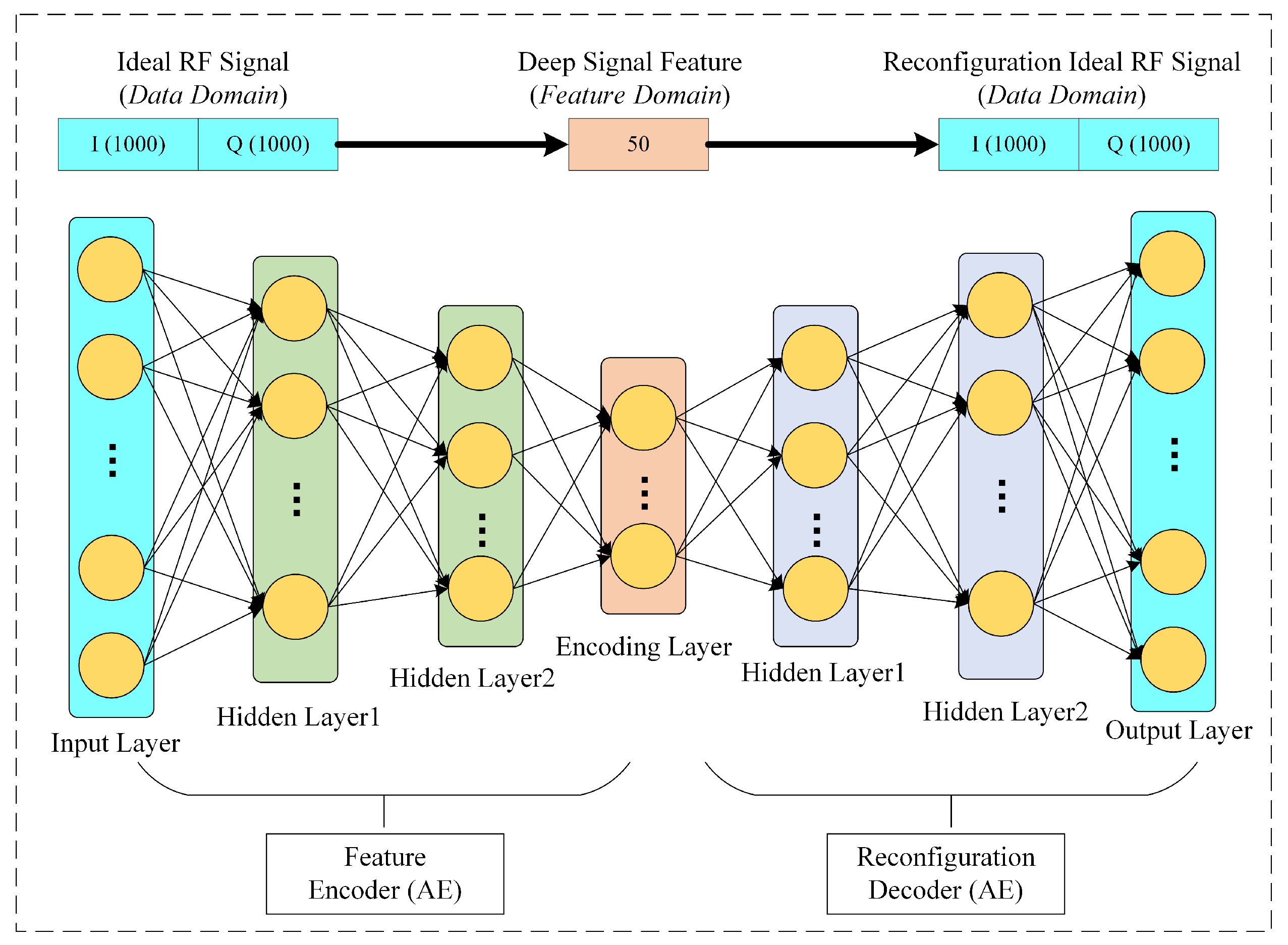
4.1. AE Network
As shown in
Figure 5, network 1 is an AE network composed of a feature encoder
and a reconstruction decoder
.
First, the input to the AE network is an ideal RF signal without RF structure information .
Then, the hidden layer dimension is set to be smaller than the input dimension. The feature encoder automatically learns the compression feature of the RF signal, which is —the deep signal feature. The RF signal is then reconstructed from this feature unsupervised via the reconstruction decoder, thereby realizing the mapping from the data domain to the feature domain and then back to the data domain.
The coding and decoding process of the AE network can be described as follows:
where
represents the feature encoder parameters, and
represents the reconstruction decoder parameters.
This reconstruction method can ensure that the loss of learned feature information is minimal. To train the AE network, it is necessary to define an objective function; that is, the reconstruction error:
where
I is the number of input signal samples, and
represents the loss function. Common forms such as the mean square error (MSE) and cross entropy (CE) can be selected. This paper adopts MSE:
Therefore, the reconstruction objective function based on the MSE loss function is expressed as follows:
The exact solution of the input RF signal obtained via the AE network is as follows:
Finally, the optimization method is used to train the AE network continuously, and the trained feature encoder is saved.
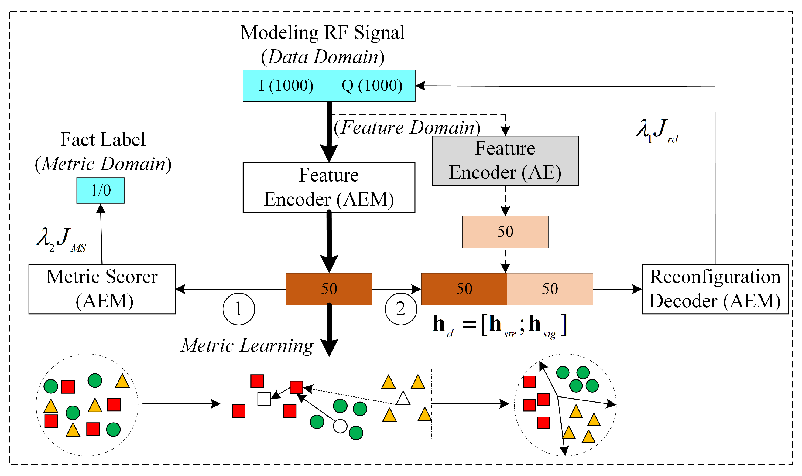
4.2. AEM Network
As shown in
Figure 6, the AEM network is composed of a feature encoder
, a reconstruction decoder
, and a metric scorer
. In the following sections, this network is described in detail, including the input signal, network structure, and objective function.
4.2.1. Feature Encoder
First, the feature encoder of the AEM network has the same design as the feature encoder of AE, but the input is an RF signal carrying RF structure information.
Then,
automatically learns the deep RF structure feature
of the RF signal. The mapping between the data domain and feature domain is realized:
where
represents the feature encoder parameter.
After this steap, is fed into the two branches of the reconstruction decoder and the metric scorer. The RF signal is reconstructed in the feature domain unsupervised, aiming at obtaining stable extracted deep RF structure features. In addition, the similarity score is computed using the supervised metric method in the feature domain, aiming at obtaining the good separability of the extracted deep RF structure features.
4.2.2. Reconstruction Decoder
The RF signal
is input into the feature encoder of the AEM network and the feature encoder of the trained AE network to obtain deep RF structure features and deep signal features. In the reconstruction decoder,
and
are spliced in parallel as the input of the reconstruction decoder:
The reconstruction decoder reconstructs the RF signal
from
in an unsupervised manner, thereby realizing the mapping between the feature domain and data domain. The decoding process can be described as follows:
where
represents the reconstruction decoder parameter.
In addition, the reconstruction objective function is designed based on the MSE loss function:
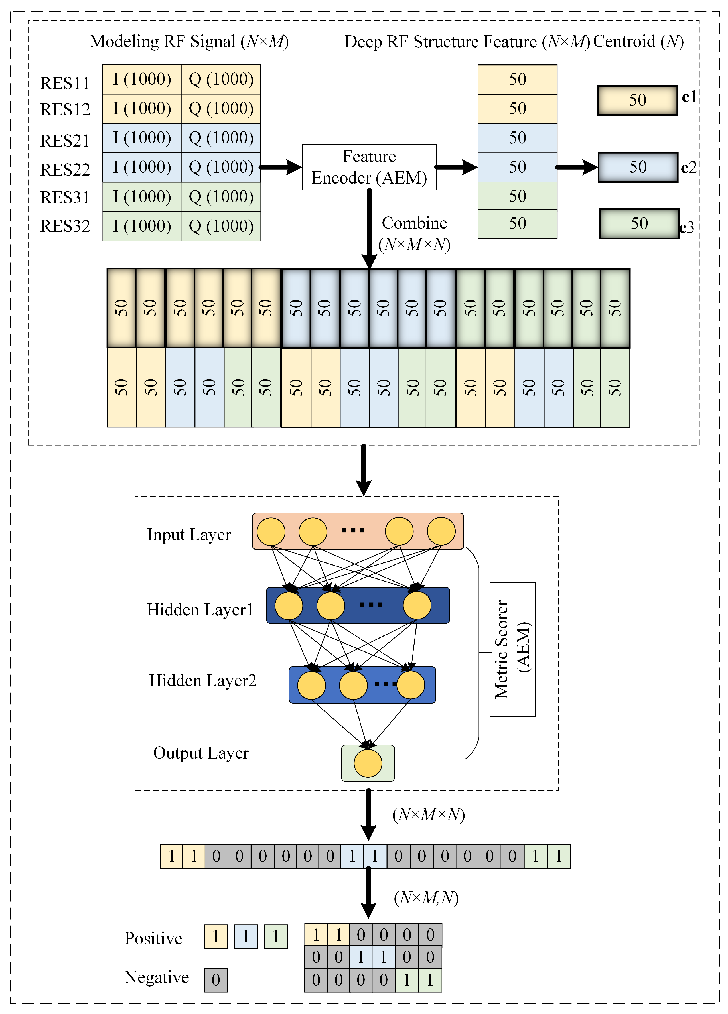
4.2.3. Metric Scorer
Metric learning is one of the core problems of pattern recognition. To measure the similarity between samples, metric learning can also be considered as similarity. Its purpose is to minimize the distance between the same class of samples and increase the distance between different classes of samples. Therefore, the metric learning method selected in this paper aims to improve the feature domain separability of the extracted deep RF structure features.
Drawing on the design concept of the generalized end-to-end loss function [
58], the input of the metric scorer is designed as samples of a batch, including
N different classes of RES and
M samples under each class, as shown in
Figure 7.
First,
RF signals
are acquired to build a batch:
which are then fed into the feature encoder to extract their
deep RF structure features.
represents the deep RF structure features of the
i-th RF signal of the
j-th class of RES.
Then, the centroids of the deep RF structure features of the
j-th class of RES are calculated:
where
.
In addition, it is noted that the deletion of a term when calculating the centroid of the real RES can stabilize the training process and help avoid trivial solutions [
58]. Therefore, when
, the centroid of deep RF structure features is calculated using the following formula:
In addition, the deep RF structure features
of each RF signal and the centroids
of all classes are combined in series to form
RF feature pairs as the input of the metric scorer.
The similarity score of each RF feature pair is calculated using a metric scorer, and the mapping between the feature domain and metric domain is realized:
where
represents the metric scorer parameter.
In the metric scorer, for each class of RES, each deep RF structure feature in
M samples should have a higher similarity relative to the centroid of the deep RF structure feature in the same class, and it is far from the centroid of deep RF structure features in other classes. As shown in
Figure 7, the expected effect of the metric scorer is that it introduces a larger value with respect to the colored part of the similarity score matrix, while the gray part has a smaller value.
When designing the objective function, first, the
similarity score is mapped into an
similarity score, and the vector
of each row of the matrix is as follows:
The SoftMax function is applied to the similarity score of each column so that the score is a scalar in the range of
; then, the similarity score is regressed to the CE loss function, and the score objective function of a sample of the metric scorer is as follows:
where the first term is the loss function of positive samples, and the second term is the loss function of negative samples.
That is, for , makes the output of the metric scorer equal to 1, indicating that the features and feature centroid in the RF feature pair belong to the same class of RES (positive samples; that is, the same or different operating parameters of the same class of RES). Otherwise, the output is equal to 0, indicating that the features and feature centroid of the RF feature pair do not belong to the same class of RES (negative samples). The objective is to make the network reduce the distance between the RF signals of the hetero-mode operating parameters under the same class of RES in the feature domain during the learning process and increase the distance between the RF signals of different classes of RES in the feature domain, thereby improving the feature domain separability of the deep RF structure features.
Finally, the score objective function of a batch of the metric scorer is as follows:
4.2.4. Objective Function
In the AEM network, the feature encoder, reconstruction decoder, and metric scorer are regarded as a single neural network, and the three subnetworks are jointly trained in end-to-end training to optimize them relative to one direction. As a result, the inconsistency in the process of separate network training can be eliminated, and the best network can be obtained. Therefore, the overall objective function of the AEM network is as follows:
where
and
represent the proportion weight of the reconstruction objective function and score objective function, respectively. In this paper, the two objective functions are regarded as the same important component, namely,
. Finally, the appropriate optimization method is selected to optimize the network.
4.3. RES Inversion Method
The flow chart of the RES inversion method is shown in
Figure 8, and the overall process of RES modeling and RES conversion can be observed in the figure, which shows the training process of the AE network and AEM network, as well as the testing process of the AEM network. The specific steps are summarized as follows.
Building datasets:
Modeling training dataset: yhe three classes of RES modeled above are used to generate the training dataset under hetero-mode operating parameters, and corresponding labels are added;
Ideal training dataset: yhe ideal training dataset is generated based on the operating parameters of the modeling training dataset;
Test datasets: using the three classes of RES models, closed-set test datasets and open-set test datasets are generated.
Data preprocessing:
In-phase/quadrature (I/Q) data are extracted from complex RF signals, and they are concatenated for normalization. The sampling rate is set to , and the pulse width is ; thus, the number of complex RF signal sampling points is 1000. Therefore, the number of input nodes is .
Training stage: The specific training process of the network is described as follows:
- (a)
AE network: The ideal training dataset is used as input to the AE network. Both the setup feature encoder and the reconstruction decoder have two hidden layers. The number of output nodes of the feature encoder is set to 50; thus, the number of nodes of each layer of the feature encoder is . The number of nodes in each layer of the reconstruction decoder is . The objective function is used to train the AE network. The adaptive moment estimation (Adam) optimizer is used for network training. The learning rate is set to 0.0001, and the batch size is set to 60. The network parameters are selected and determined empirically after many experiments; the parameters of the feature encoder and the reconstruction decoder are obtained, and the trained feature encoder is saved.
- (b)
AEM network: The modeling training dataset and corresponding labels are used as inputs to the AEM network. Each of the setup feature encoder, the reconstruction decoder, and the metric scorer contain two hidden layers. The number of feature encoder output nodes is set to 50. The number of nodes in each layer of the feature encoder is , while the number of nodes is for each layer of the reconstruction decoder, and is observed for each layer of the metric scorer. The objective function is used along with the Adam optimizer to train the AEM network. The learning rate was set to 0.0001 and the batch size was set to , i.e., a batch contains three classes of RES with 20 samples per class. The network parameters are selected and determined empirically after many experiments. The parameters of the feature encoder, the reconstruction decoder, and the metric scorer were obtained, and the trained feature encoder and metric scorer were saved.
- (c)
Centroid database: In the last epoch, the centroid of each class of deep RF structure features calculated by each batch is saved and averaged to generate a centroid database, which is used as the centroid of deep RF structure features in the test phase.
Test stage:
The network is tested using the test dataset. First, the test data are input into the feature encoder of the AEM network to extract the deep RF structure features. For each class in the centroid database, class centroids are then combined together and input into the metric scorer to calculate the similarity score. The maximum matching score corresponds to the class of RES, and the RES inversion is therefore realized.
Figure 8.
Flowchart of the RES inversion method.
Figure 8.
Flowchart of the RES inversion method.
5. Experiments
5.1. Simulation and Analysis of the Modelled RF Signal
First, the spurious information introduced by DDS signal source models with different modulation types is verified using experiments. The frequency of the reference clock source is , the number of bits in the phase accumulator is , the number of bits for phase truncation is , the pulse width is , and the sampling rate is . Thus, , , and . According to the parameters set in the model, and can be obtained. The frequency variation range of the LFM is 20∼30 MHz.
Figure 9 shows four modulation types of source signals generated by the ideal signal source and four DDS source models. It can be observed from the spectrum that the phase truncation error of the DDS model has a certain influence on the spectrum of the four modulation type signals. In addition, the presence of spurious information can be clearly observed in the spectrum.
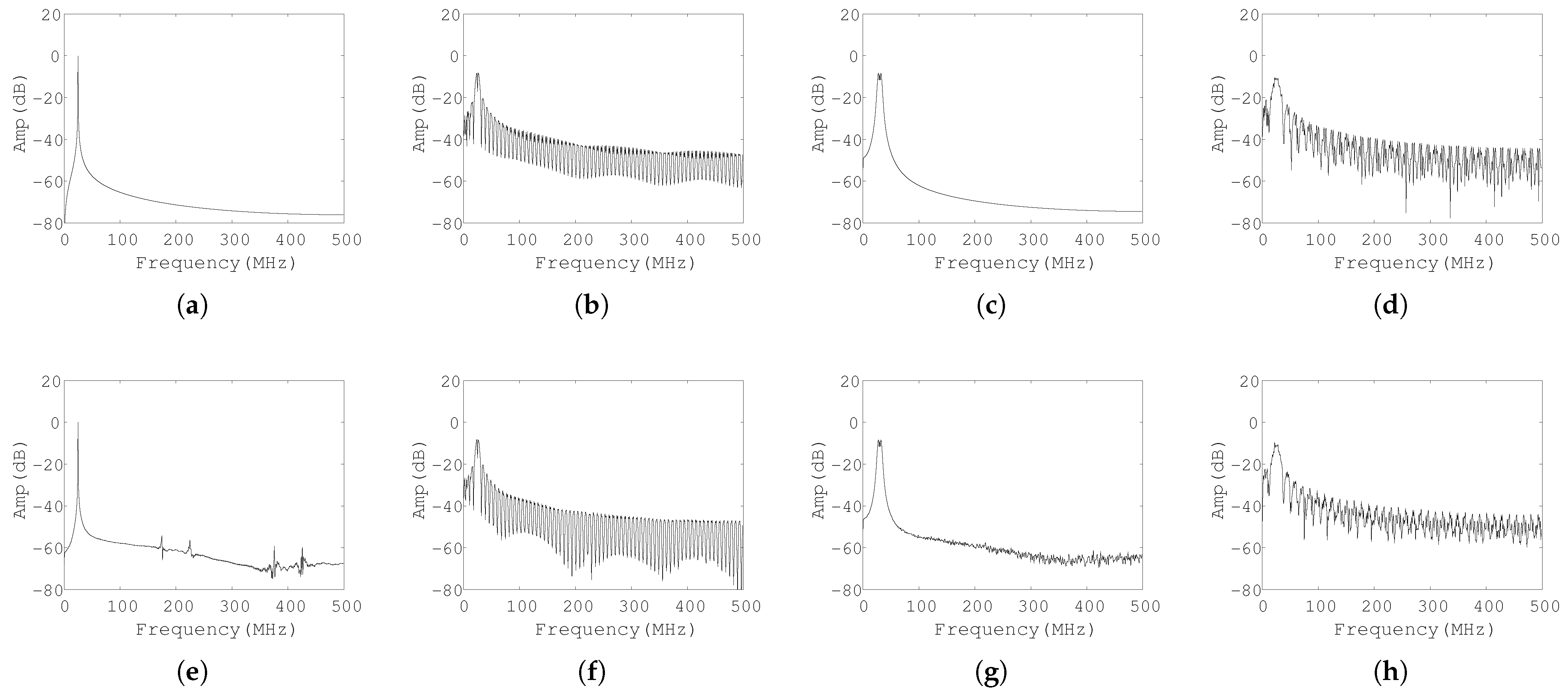
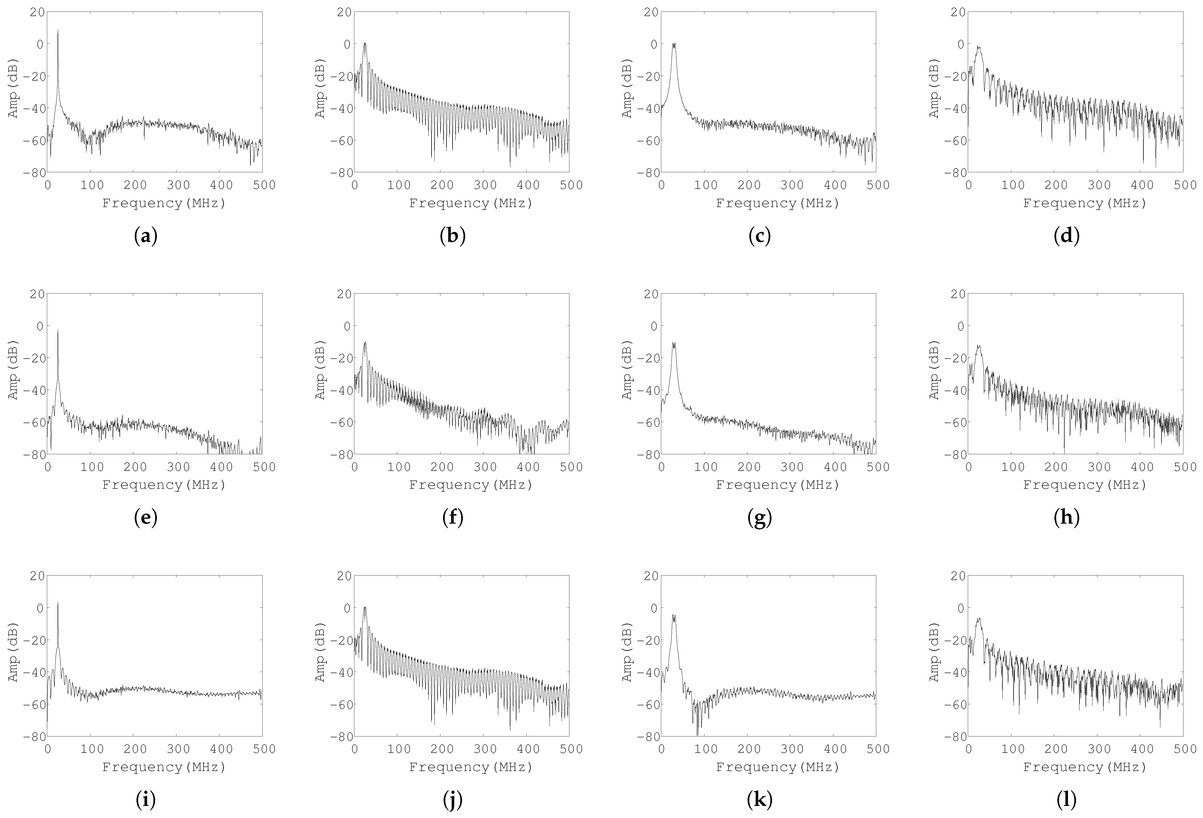
The RF structure information of the different classes of RES models is then verified using experiments.
Figure 10 illustrates the spectrum diagram of the RF signals produced by different classes of RES models. It is clear that the three classes of RES models exhibit distinct differences in the spectrum purity of RF signals of the four modulation types. Each RF signal carries different RF structure information, with the RF signal generated by the RES1 model having the smallest amount of RF structure information. This is because the amplifier of the RES1 model is relatively ideal and only exhibits one stage of amplification. The measured S parameter is used for the amplifier modeling of RES2 and RES3 models, and the RF structure information is obvious. The structure differences caused by the usage mode, working principle, and material composition of each module are also verified. The generated RF signal also carries various levels of unique RF structure information. In addition, there are obvious differences in the spectrum purity of RF signals with various modulation types under the same RES model, and each RF signal carries different signal information.
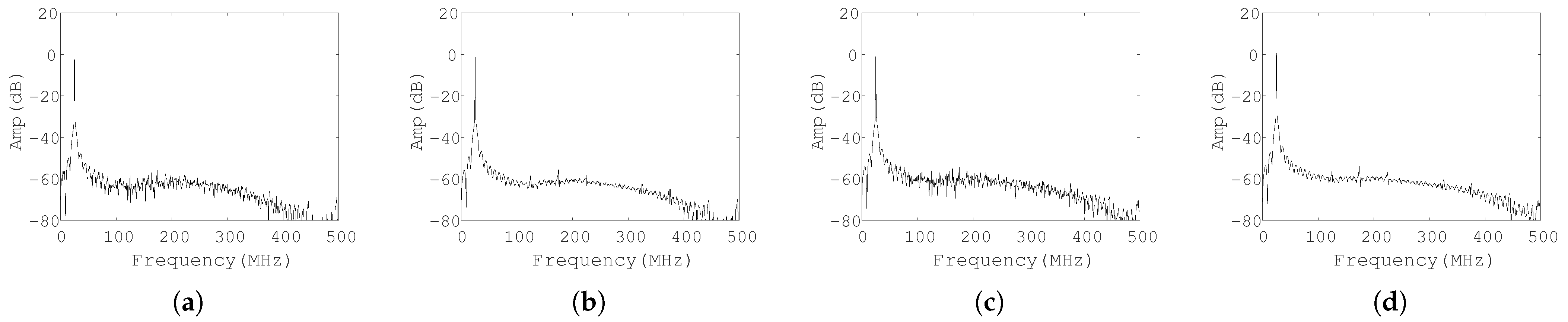
Finally, the individual information introduced by different REI models under the same class of RES models is validated experimentally. As shown in
Figure 11, as observed from the spectrum of RF signals (DDS_CW) generated by four different REI models under the RES2 model, the RF signals of four different REI models under the same RES2 model carry different individual information, and there is less individual information than RF structure information, reflecting the subtle differences among individuals.
5.2. Hetero-Mode Operating Parameter Dataset
In the modeling training dataset, there are RF signals of three modulation types relative to the DDS_CW, DDS_LFM, and DDS_BPSK models. More precisely, the DDS_CW signal is set to different frequencies, the DDS_LFM signal is set to different initial frequencies and bandwidths, the DDS_BPSK signal is set to different carrier frequencies, and the RF link model is set to different input powers. The operating parameters of the training dataset are shown in
Table 2. The number of RF signal samples of each modulation type of each RES model is 2000. Gaussian noise with
is then added to each RF signal, and the simulation sample size is
18,000 with respect to the hetero-mode operating parameters of the modeling training dataset as well as the corresponding simulation of the ideal training dataset. Each sample in the modeling training dataset is then supplemented with a corresponding label in the one-hot encoding mode, and the label is a
vector. To obtain the unbalanced dataset of hetero-mode operating parameters, these parameters will be randomly selected. For instance, there will be
combinations of operating parameters under the DDS_LFM model.
The test dataset is divided into a closed-set test dataset and open-set test dataset. The operating parameters of the closed-set test dataset and the training dataset are the same, but these data and their operating parameters have not participated in the model’s training, i.e., the network has not perceived these data. The operating parameters of the open-set test dataset are different from those of the training dataset; that is, the network has never seen these operating parameters nor participated in network training. As shown in
Table 3, the test dataset is divided into a closed set and five different open-set test datasets, which are composed of F change; B change; P change; MT change; and MT, F, and P change. The number of RF signal samples for each modulation type under each class of RES models is 40. Gaussian noise with different
is also added. For instance, there are
samples in the closed-set test dataset.
5.3. Feature Extraction Performance and Analysis of the AEM Network
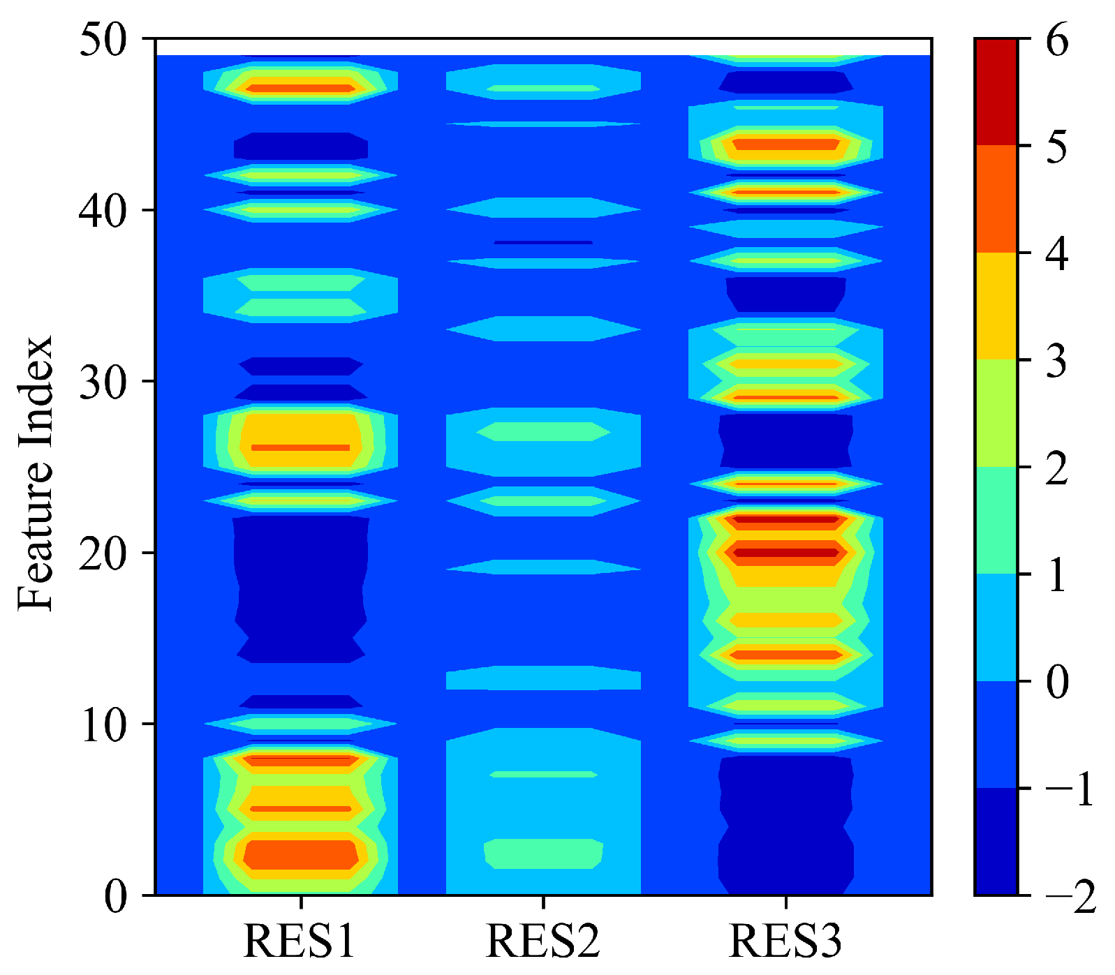
First, to verify whether the AEM network can extract the RF structure information carried by RF signals under hetero-mode operating parameters, the centroids of the deep RF structure features of three classes of RES saved by the AEM network after training are visualized and analyzed in the form of a heat distribution map [
59].
Figure 12 shows a visualization of the 50-dimensional deep RF structure feature centroid combination of three classes of RES extracted from the AEM network. It can be observed that the centroids have obvious differences. The feasibility and uniqueness of extracting deep RF structure features from the AEM network are verified. Therefore, these deep RF structure features can be used for RES inversion.
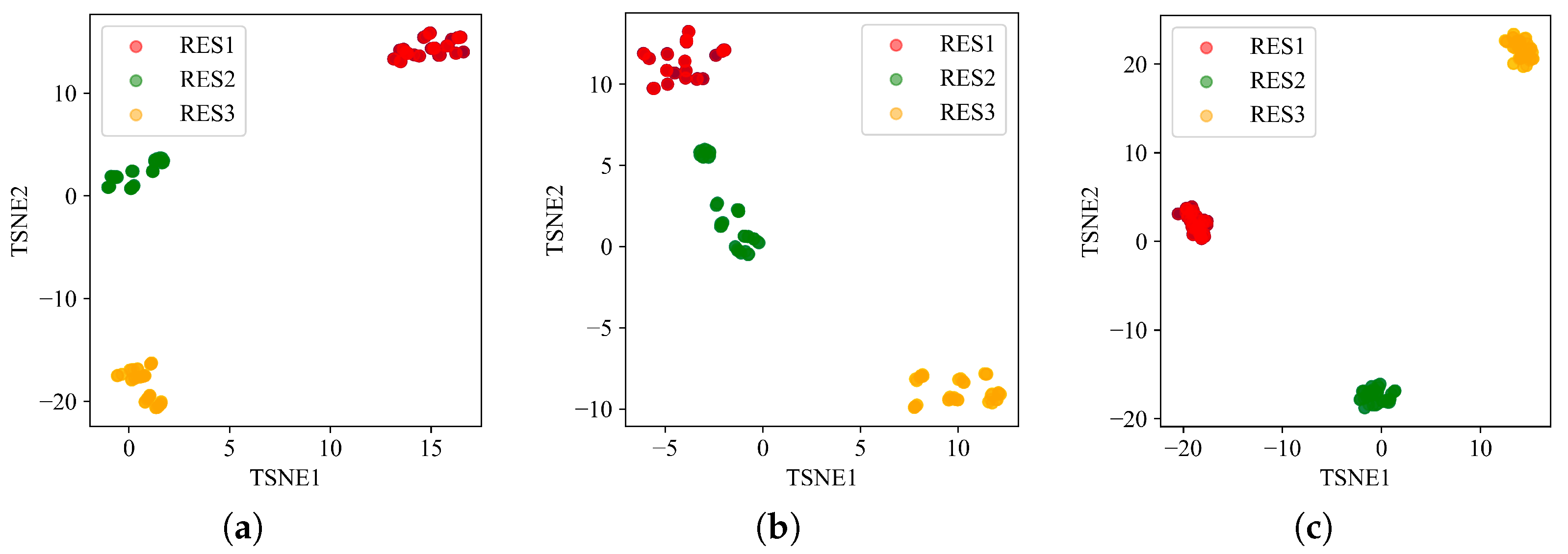
Sample data with
were selected in the closed-set test dataset to further verify whether the deep RF structure features extracted by the AEM network in this paper have good separability under hetero-mode operating parameters. The deep RF structure features extracted by the AEM network have reduced dimensionality using t-SNE [
28] technology, and the distribution of deep RF structure features is visualized in two-dimensional space.
Figure 13a–c show the visualization of the deep RF structure feature distribution of three classes of RES extracted by the AEM network using CW, BPSK, and LFM modulation types, respectively. It is clear that these RF structure features have obvious separability relative to different modulation types, and the separability effect is the best under the LFM modulation type.
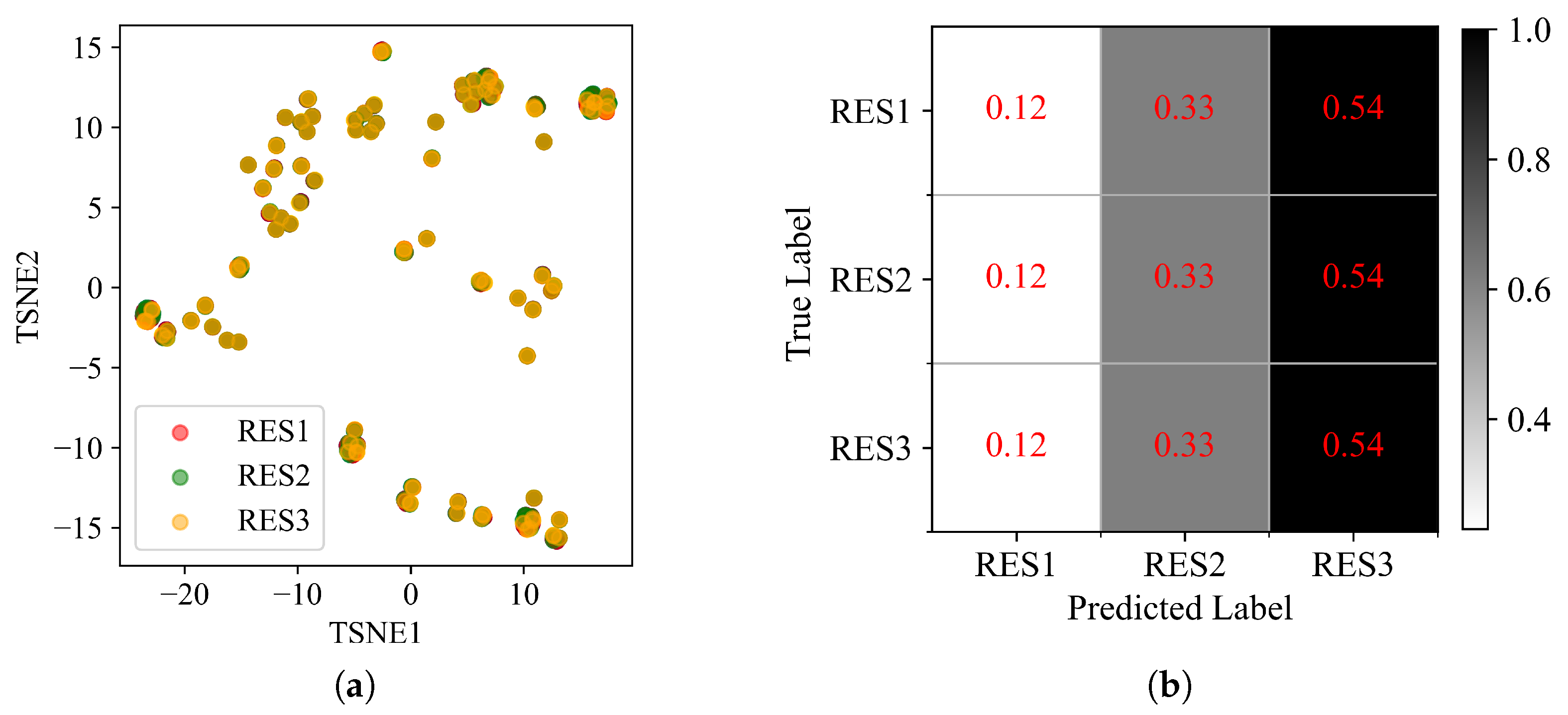
Finally, the stability of the deep RF structure features extracted using the AEM network was further verified under hetero-mode operating parameters. The ideal test dataset without RF structure information under the operating parameters corresponding to the closed-set test dataset (
) was simulated and input into the AEM network to verify its separability and inversion rate. This is a mathematical paradox; if the AEM network cannot clearly distinguish between ideal test data without RF structure information, this indirectly proves that it is extracting deep RF structure features rather than deep signal features.
Figure 14a is a visualization of a two-dimensional space that uses t-SNE technology to reduce the dimension of extracted features. It can be observed that using the ideal test dataset, the features extracted by the AEM network are not separable.
Figure 14b shows the inversion confusion matrix, where it can be observed that the AEM network no longer has the inversion performance. Therefore, the feasibility and stability of deep RF structure features extracted by the AEM network were indirectly proven.
5.4. Comparison and Analysis of the Generalization Performance of Different Networks
Since RES inversion is a new problem, there are no comparable methods in the published literature. Therefore, in this section, the generalization performance of the AEM network is evaluated via experimental comparisons with some relevant baseline neural networks. Due to space limitations, only some of the experimental results from the test dataset are shown. The baseline network1 is a deep neural network (DNN): it consists of a feature encoder with two hidden layers and a SoftMax classifier (i.e., a feature encoder and a classifier without a reconstruction decoder); the baseline network2 is a CNN: it includes three convolutional and pooling layers, two DNN layers, and a SoftMax classifier. These two networks are used to demonstrate the role of including a reconstruction decoder in this AEM network. Another network used for comparisons is the SAE network: it consists of three stacked AE networks and a SoftMax classifier (i.e., a feature encoder, a reconstruction decoder, and a classifier). The network is trained by initializing and fine-tuning layer by layer. This network is used to demonstrate the function of the metric scorer in the AEM network. Except for the differences in the network’s structure design, the other conditions are the same as the proposed AEM network.
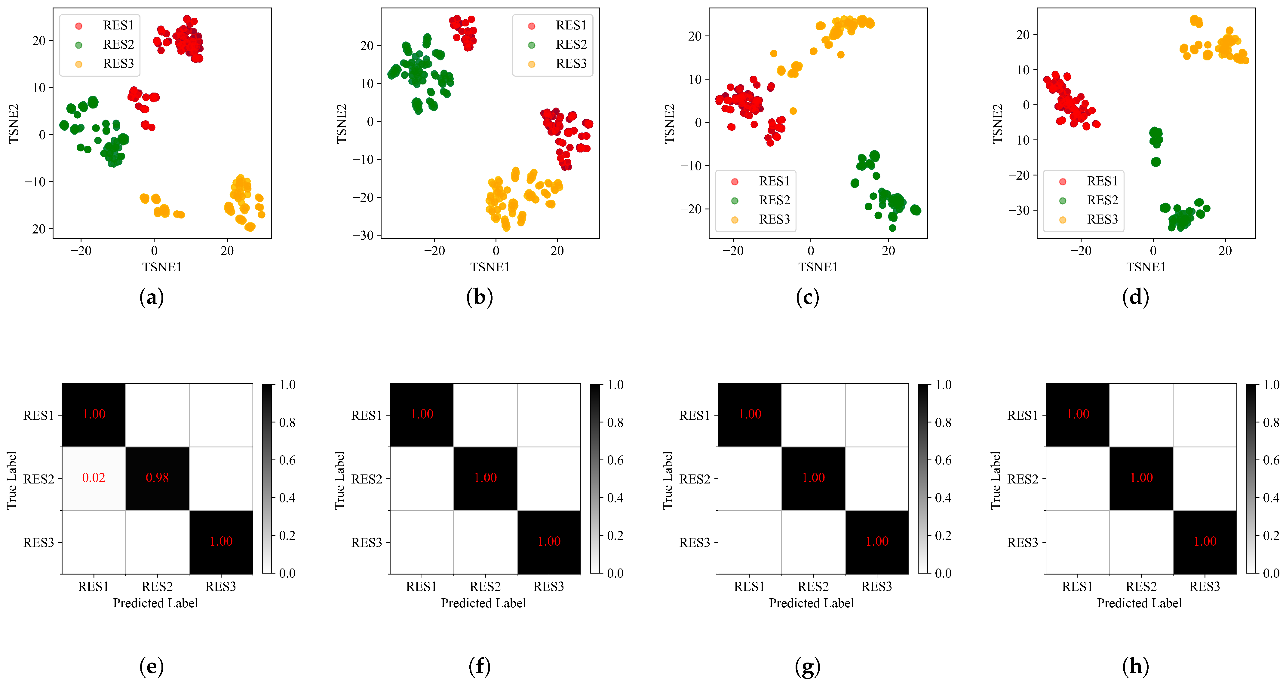
In the closed-set test dataset, samples with
are selected to verify the performance of the comparison network and the proposed AEM network.
Figure 15a–d visualizes the four networks using t-SNE technology to reduce the extracted deep RF structure features in two-dimensional space. It can be observed that the features extracted by the four networks are distinguishable. However, since the DNN, CNN, and SAE networks use the SoftMax classifier, the spacing between the same class is large, and the boundary of different classes is blurred. The AEM network makes the distance between the same class smaller, the distance between different classes larger, and the boundary clearer using metric learning. Therefore, features extracted by the AEM under hetero-mode operating parameters have higher separability, and samples mixed with three different modulation types of the same class of RES are grouped together.
Figure 15e–h illustrates the inversion confusion matrix of the four networks. As observed, all four networks exhibit good inversion performance.
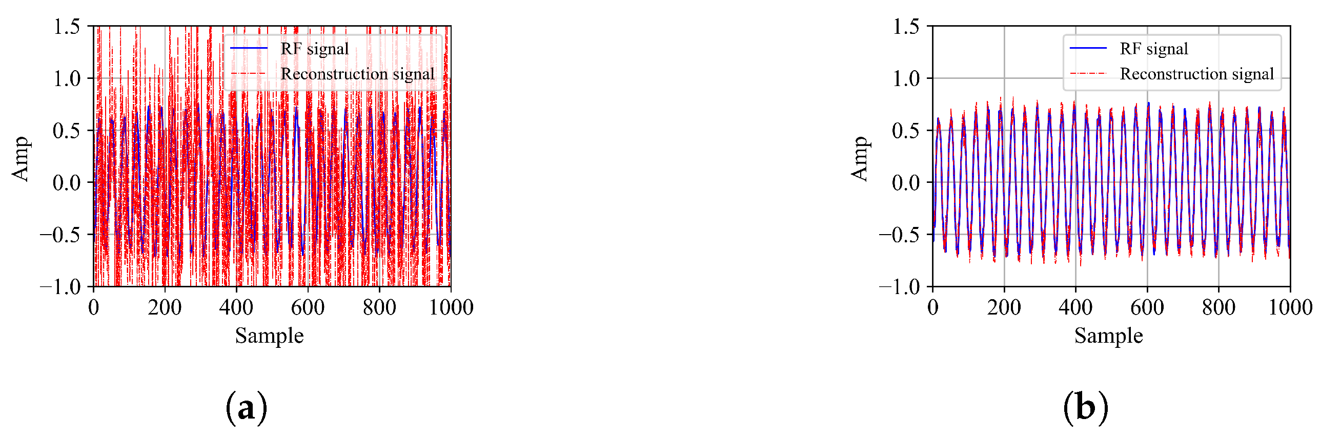
Due to the lack of reconstruction performance in DNN and CNN networks,
Figure 16a,b only shows the time-domain reconstructions of SAE and AEM networks. It can be observed that the SAE network has poor reconstruction performance. The AEM network has good reconstruction performance, and it can constrain the features to make them more stable.
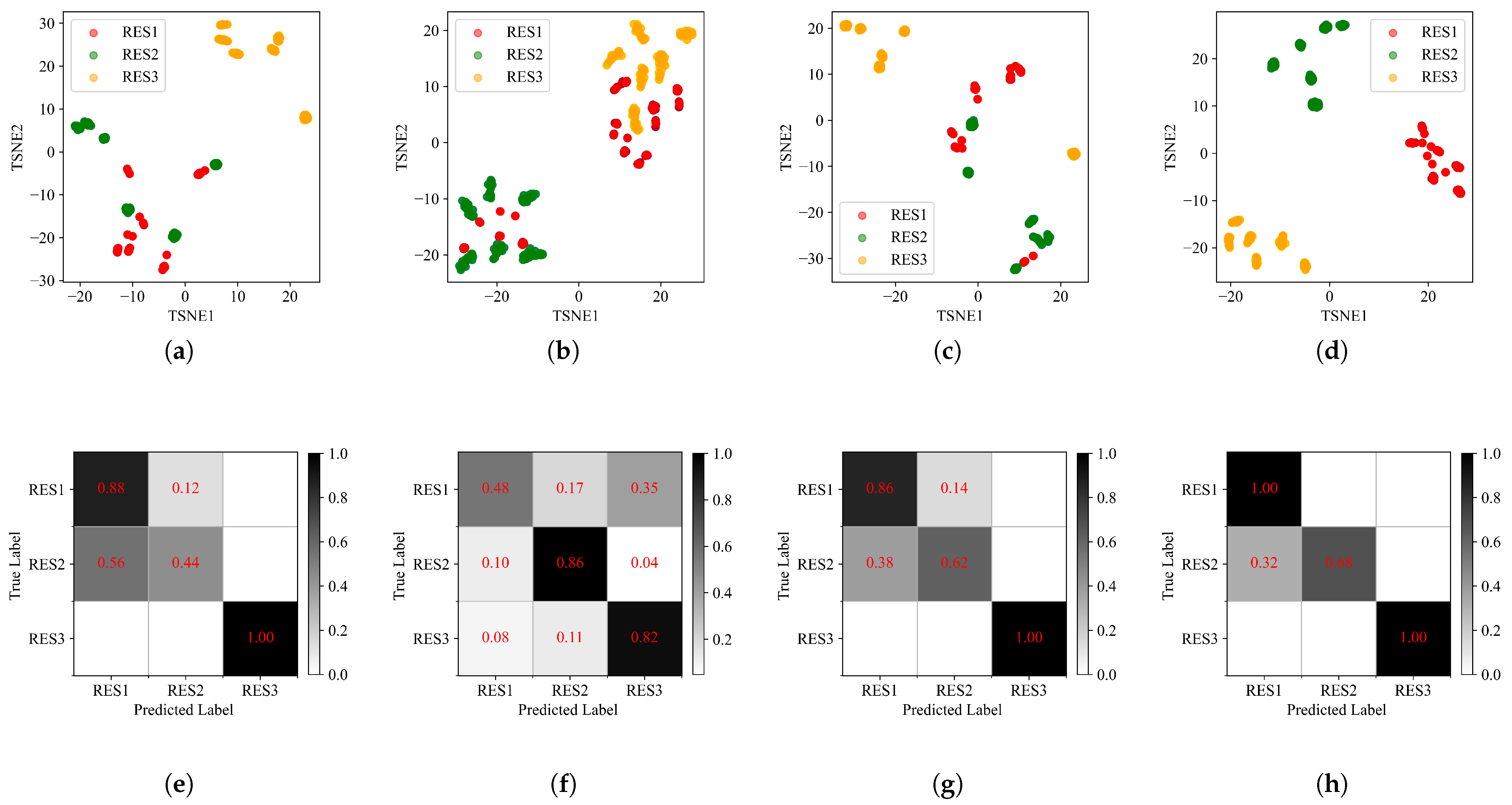
In the open-set test dataset4, samples with
are selected to verify the performance of the comparison network and the proposed AEM network under unknown operating parameters (MT).
Figure 17a–d visualizes the four networks using t-SNE technology to reduce the extracted deep RF structure features in two-dimensional space. It can be observed that in DNN, CNN, and SAE networks, the distance between elements of the same class is large, the boundary between different classes is fuzzy, and even aliasing occurs between classes. The AEM network can still make the spacing within the same class smaller, the spacing between different classes larger, and the boundary clearer under unknown operating parameters.
Figure 17e–h depicts the inversion confusion matrix of the four networks, with the total inversion rates being 77%, 72%, 82%, and 89%, respectively. It can be observed in the figure that the inversion rates of the DNN, CNN, and SAE networks are low, while the proposed AEM network can also obtain satisfactory inversion performance under unknown operating parameters. In addition, the inversion rates of RES1 and RES3 can still reach 100%, but the inversion rate of RES2 is lower than that of RES1 and RES3, and part of RES2 is inverted into RES1. This could be because RES1 and RES2 models are more similar—i.e., their structure difference is small—while the RES3 model is significantly different due to its larger RF structure information, which further explains the consistency with previous RES modeling and spectrum analyses.
5.5. Robust Performance and Analysis of the AEM Network
Next, the robustness of the proposed network is verified under different SNRs, and experiments are conducted separately relative to all the above test datasets. The inversion rates under different SNRs are shown in
Table 4. It is clear that the proposed network exhibits higher inversion rates under both closed- and open-set test datasets. Particularly under different unknown operating parameters, the inversion performance of the network is still relatively stable as the SNR decreases gradually. When the SNR is −10 dB, the inversion rate can still reach more than 80%, which proves the anti-noise performance of the proposed AEM network. In addition, in the training stage, the network only learns the data in the environment. In the environment of low SNR without training, the deep RF structure features extracted by the AEM are still unaffected by the unknown low-SNR environment, which further demonstrates that AEM has high robustness and generalization performances.
6. Discussion
The results of the above comparison experiment demonstrate that although DNN, CNN, and SAE networks have good inversion performances using the closed-set test dataset, their inversion rate is greatly reduced relative to the open-set test dataset because the features extracted from the known operating parameters of the network do not have good stability and separability, which greatly affects the network via changes in the operating parameters. With unknown operating parameters, the generalization performance of the network is reduced. The proposed AEM network can extract features with the essence of RF structure information by means of the joint optimization of metric learning and reconstruction learning to obtain better inversion performance, and such features have good stability and separability. Furthermore, the network exhibits good generalization performance relative to unknown operating parameters.
7. Conclusions
In this paper, an RES inversion method based on a dual neural network is proposed in complex situations. Using the method of joint unsupervised and supervised training and the powerful nonlinear processing ability of neural networks, the extracted deep RF structure features have good stability and separability, and the RES is then inverted via RF signals in the feature domain. Combined with deep learning technology, RES inversion is studied from a new perspective. The inversion rate and visualization feature map experiments show that the proposed method exhibits high inversion performance in complex situations and high robustness performance under low-SNR conditions. Even under unknown operating parameters, the network also has strong generalization performances. Via RES inversion, the hostile radar can be deeply recognized, which helps in identifying its performance, threat level, and combat capability and efficiently supports cognitive reconnaissance of the electronic countermeasure system. In the future, we will further study RF feature extraction technologies and RES inversion methods using real data in complex situations.


