MuA-SAR Fast Imaging Based on UCFFBP Algorithm with Multi-Level Regional Attention Strategy

Abstract

Multistatic airborne SAR (MuA-SAR) benefits from the ability to flexibly adjust the positions of multiple transmitters and receivers in space, which can shorten the synthetic aperture time to achieve the required resolution. To ensure both imaging efficiency and quality of different system spatial configurations and trajectories, the fast factorized back projection (FFBP) algorithm is proposed. However, if the FFBP algorithm based on polar coordinates is directly applied to the MuA-SAR system, the interpolation in the recursive fusion process will bring the problem of redundant calculations and error accumulation, leading to a sharp decrease in imaging efficiency and quality. In this paper, a unified Cartesian fast factorized back projection (UCFFBP) algorithm with a multi-level regional attention strategy is proposed for MuA-SAR fast imaging. First, a global Cartesian coordinate system (GCCS) is established. Through designing the rotation mapping matrix and phase compensation factor, data from different bistatic radar pairs can be processed coherently and efficiently. In addition, a multi-level regional attention strategy based on maximally stable extremal regions (MSER) is proposed. In the recursive fusion process, only the suspected target regions are paid more attention and segmented for coherent fusion at each fusion level, which further improves efficiency. The proposed UCFFBP algorithm ensures both the quality and efficiency of MuA-SAR imaging. Simulation experiments verified the effectiveness of the proposed algorithm.

1. Introduction

Synthetic aperture radar (SAR) is widely used in civil and military fields benefiting from its all-day, all-weather working capability [1,2,3,4]. SAR utilizes the relative motion between the radar platforms and the target to form a virtual large aperture, thus to obtain high-resolution images [5,6]. However, limited by the imaging mechanism, there will be blind areas in the forward-looking direction [7,8,9]. A Multistatic Airborne SAR (MuA-SAR) system usually includes multiple transmitters and receivers. By flexibly scheduling these radar platforms, the imaging tasks with almost no blind areas can be completed and information different from that of monostatic SAR can be obtained [8,9,10]. Additionally, the MuA-SAR system can achieve the required imaging resolution in a shorter time through data fusion.

Because each radar platform in the MuA-SAR system is placed in a different position in space, the echo data of different platforms have different viewing angles [11,12,13]. Therefore, to realize the effective fusion of data from different platforms, the imaging processing method is required to be adaptive to the different spatial configurations and trajectories of the MuA-SAR system [14,15]. In addition, the introduction of multiple platforms brings a huge amount of echo data, which puts forward higher requirements for the efficiency of imaging algorithms. Many SAR imaging algorithms are proposed, and

Table 1. Summary of the advantages and disadvantages of existing representative algorithms.

Algorithm	Advantage	Disadvantage
RDA/CSA	Uniformly process the spatial variability, High efficiency	Complicated space-variant problems for multiple platforms
PFA	Minimize processing load	Approximate calculation, Not applicable to wide swath scenes and multiple platforms
Omega-K	Accurately calculate geometric relationships	Requires specific configuration and straight trajectory
BP	Accurate, Suitable for any configuration and trajectory	High computational complexity
FFBP	High efficiency	Interpolation leads to error accumulation for multiple platforms
CFFBP	Noninterpolation, High efficiency	Not suitable for multiple platforms

summarizes the advantages and disadvantages of some representative algorithms. The existing FFT-based imaging algorithms, including the range-Doppler algorithm (RDA) and chirp scaling algorithm (CSA), are widely used and deeply studied. They can uniformly process the spatial variability of the echo data in the range Doppler domain, which has high computational efficiency. When introducing multiple radar platforms, it will face more complicated space-variant problems, which will lead to algorithm mismatch [16,17,18]. Wavenumber domain algorithms, such as the polar format algorithm (PFA), can minimize processing load, but these algorithms have approximate processing when calculating the range history, which will lead to image quality degradation for wide swath scenes [19,20]. As for the frequency domain algorithm, such as the omega-K algorithm, it is accurate in the calculation of the imaging geometric relationship, but it requires platforms to have a specific configuration and a straight trajectory, which weakens the flexibility of the MuA-SAR system [21,22]. In addition, most of these algorithms need to be interpolated in the frequency domain, and the errors caused by the interpolation process will accumulate along with the fusion of multi-platform data, thus degrading the focusing performance [23,24,25]. Therefore, it is necessary to propose a novel MuA-SAR fast imaging algorithm that is insensitive to the spatial configuration and trajectory of platforms and avoids interpolation operation as much as possible.

The back projection (BP) algorithm is a widely used time domain algorithm that utilizes point-by-point coherent accumulation to achieve high-resolution imaging. It has a certain adaptability to any spatial configuration and trajectory. However, point-by-point calculation and back projection bring a huge computational burden [26,27,28]. Many efforts have been made to improve the efficiency of the BP algorithm [29,30]. AF Yegulalp et al., proposed the fast BP (FBP) algorithm, which divides the full aperture into multiple sub-apertures, and establishes independent local polar coordinate systems for each sub-aperture to complete the projection and obtain multiple sub-images. Then, the sub-images are coherently fused to obtain images with higher azimuth resolution [31,32]. Based on the FBP algorithm, LMH Ulander et al. proposed a fast factorized back projection (FFBP) algorithm using aperture factorization to further improve efficiency, which needs to be at the expense of reducing focusing performance [33,34,35]. Therefore, the FFBP algorithm needs to seek a compromise between performance and efficiency. S Zhou et al., proposed an improved FFBP method based on an orthogonal elliptical polar (OEP) coordinate. A narrower WS distribution is obtained, which improves the efficiency of the algorithm to some extent, but it still does not avoid interpolation operation [36]. L Zhang et al., established a unified polar coordinate (UPC) system to complete the projection of sub-apertures, and proposed accelerated fast back projection (AFBP) [37]. Based on UPC, H Sun et al. proposed a wavenumber domain fast back projection (WFBP) method to achieve fast imaging of monostatic and bistatic SAR systems [38]. They improved imaging efficiency and performance by fusing wavenumber spectra (WS). Y Guo et al., proposed an algorithm called high-squint and high-dive accelerated factorized back-projection (HSHD-AFBP), which can not only improve the imaging quality but also expand the image width [39]. Q Dong and Y Li et al., proposed a Cartesian FFBP (CFFBP) for monostatic and bistatic SAR, which are noninterpolation methods, and the imaging efficiency is improved [40,41,42]. Although the above improved BP-based algorithms establish polar coordinate systems or Cartesian coordinate systems, they are all local coordinate systems for the currently analyzed monostatic or bistatic SAR systems. However, when faced with more platforms and angles of view of echo data, these methods cannot be used, because of the phase difference caused by each local coordinate system. Therefore, it is necessary to propose a unified processing method for multiple bistatic radar pairs system to improve the performance and efficiency of MuA-SAR imaging.

In this paper, a unified Cartesian fast factorized back projection (UCFFBP) algorithm with multi-level regional attention strategy is proposed for MuA-SAR fast imaging. First, a global Cartesian coordinate system (GCCS) is established for uniformly coherent imaging. Second, by analyzing the distribution principles of WS, the rotation mapping matrix is designed to realize the azimuth alignment of WS, which makes the azimuth data obtain the maximum utilization at the initial level of grid division. Then, the phase compensation factor is designed to compress the sub-aperture WS and avoid aliasing. Finally, a multi-level regional attention strategy based on maximally stable extremal regions (MSER) is designed, and only the pixels of the segmented suspected target regions at each fusion level are fused coherently. The proposed algorithm effectively reduces the number of pixels that need to be searched, projected, and fused, which can improve imaging efficiency.

The main technical contributions of this paper can be summarized as the following two aspects: On the one hand, the GCCS is established, and the rotation mapping matrix and phase compensation factor are designed to deal with the phase difference exists that between multiple bistatic radar pairs. It can uniformly process the data coherently from all platforms, while avoiding redundant operation and error accumulation caused by interpolation operation. On the other hand, the multi-level regional attention strategy based on MSER is proposed, and only the pixels in the suspected target regions are coherently fused. To avoid missing valid pixels, the suspected target regions are segmented and merged in the sub-images selected at each fusion level, which further improves the efficiency under the condition of no loss of accuracy.

The rest of this paper consists of the following sections. In Section 2, the geometric model and echo model of MuA-SAR are established. In Section 3, the distribution principles of WS is analyzed. In Section 4, the proposed UCFFBP algorithm with multi-level regional attention strategy for MuA-SAR fast imaging is introduced in detail. The simulated and experimental results are given in Section 5. Section 7 presents the conclusions.

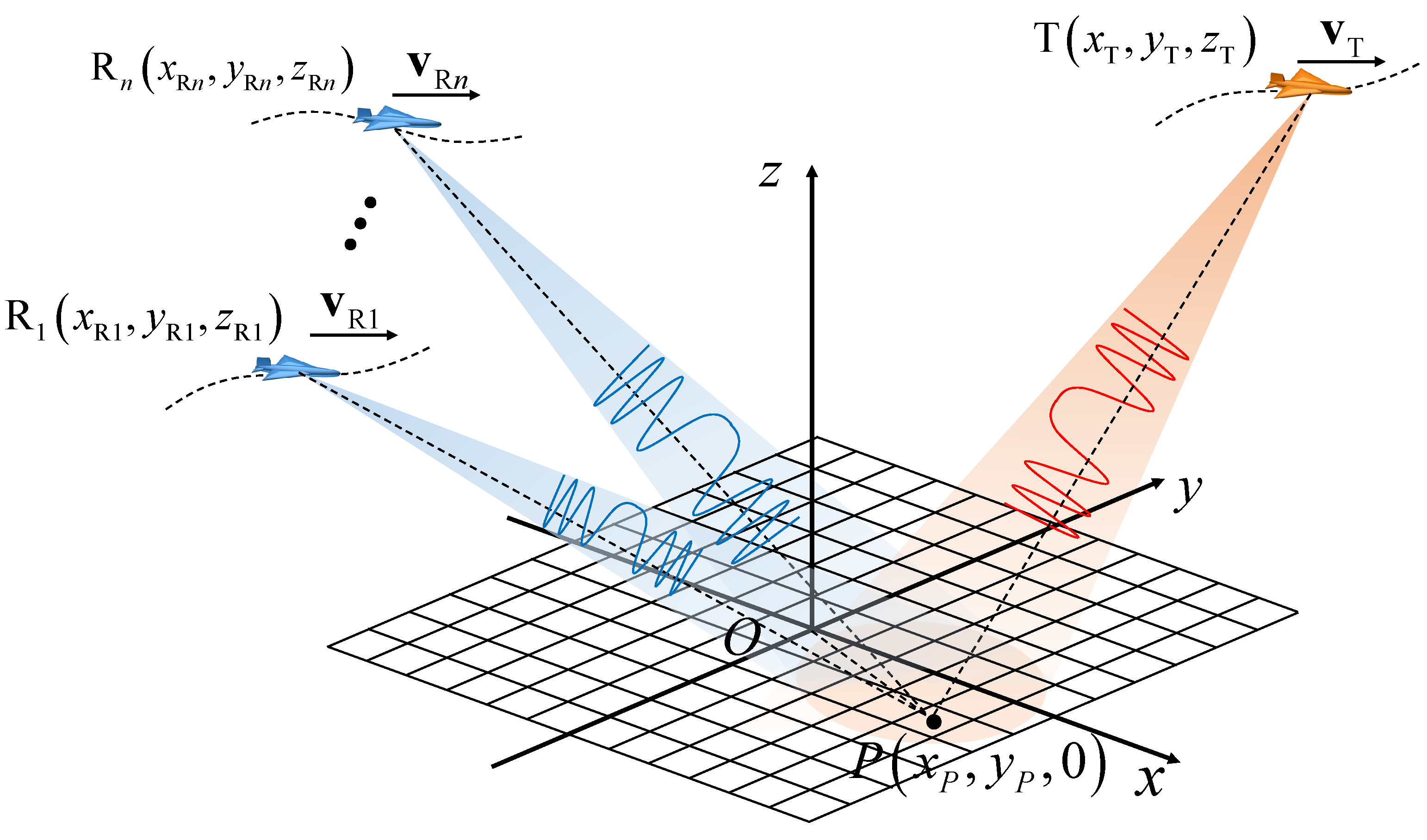
2. Echo Signal Model of MuA-SAR System

In this section, the GCCS is established first. Then, the geometric model and echo signal model of the MuA-SAR system are introduced [10,43].

A MuA-SAR system consisting of one transmitter and N receivers is taken as an example for analysis, and its spatial geometric configuration is shown in Figure 1. According to the relative position between the MuA-SAR system and the imaging scene, an appropriate origin O is selected and a GCCS $O-xyz$ is established. The initial positions of the transmitter and the $n\mathrm{th}\left(n=1,2,\dots ,N\right)$ receiver can be expressed as $\mathrm{T}\left(x_{\mathrm{T}},y_{\mathrm{T}},z_{\mathrm{T}}\right)$ and ${\mathrm{R}}_n\left(x_{\mathrm{R}n},y_{\mathrm{R}n},z_{\mathrm{R}n}\right)$. $P\left(x_P,y_P,0\right)$ is a point target in the imaging scene. The velocity vectors of the transmitter and the $n\mathrm{th}$ receiver are ${\mathbf{v}}_{\mathrm{T}}=\left(v_{\mathrm{T}x},v_{\mathrm{T}y},0\right)$ and ${\mathbf{v}}_{\mathrm{R}n}=\left(v_{\mathrm{R}nx},v_{\mathrm{R}ny},0\right)$, respectively. The coordinate variables in the $O-xyz$ can also be mapped to the spherical coordinate system, that is $\left(x,y,z\right)=\left(Rcos\alpha cos\theta ,Rcos\alpha sin\theta ,Rsin\alpha \right)$, where $R,\theta$ and $\alpha$ represent the slope distance, azimuth angle and elevation angle, respectively.

The range frequency domain echo expression of point target P can be expressed as

$$s_n\left(f_t,\tau \right)=\mathrm{rect}\left(\frac{\tau }{T_a}\right)·\mathrm{rect}\left(\frac{f_t}{B}\right)·exp\left[-j\frac{2\pi \left(f_c+f_t\right)}{c}{R}_{nP}\left(\tau \right)\right]$$

(1)

where $\tau ,T_a, B, \mathrm{and}{f}_c$ represent slow time variables, synthetic aperture time, signal bandwidth and carrier frequency of the transmitted signal, respectively. $f_t$ represents the range frequency variable and $f_t\in \left[-B/2,B/2\right]$. $R_{nP}\left(\tau \right)=R_{\mathrm{T}P}\left(\tau \right)+R_{\mathrm{R}nP}\left(\tau \right)$ is the instantaneous range history, and

$$\left\{\begin{array}{c}{R}_{\mathrm{T}P}\left(\tau \right)=\sqrt{{\left(x_{\mathrm{T}}+v_{\mathrm{T}x}\tau -x_P\right)}^2+{\left(y_{\mathrm{T}}+v_{\mathrm{T}y}\tau -y_P\right)}^2+z_{\mathrm{T}}^2}\hfill \\ R_{\mathrm{R}nP}\left(\tau \right)=\sqrt{{\left(x_{\mathrm{R}n}+v_{\mathrm{R}nx}\tau -x_P\right)}^2+{\left(y_{\mathrm{R}n}+v_{\mathrm{R}ny}\tau -y_P\right)}^2+z_{\mathrm{R}n}^2}\hfill \end{array}\right.$$

(2)

3. WS Analysis for MuA-SAR Imaging

In this section, we first analyze the distribution principles of WS. Then, the influence of different bistatic radar pairs on the consistency of WS distribution and the utilization ratio of data are derived. Finally, the aliasing phenomenon is analyzed.

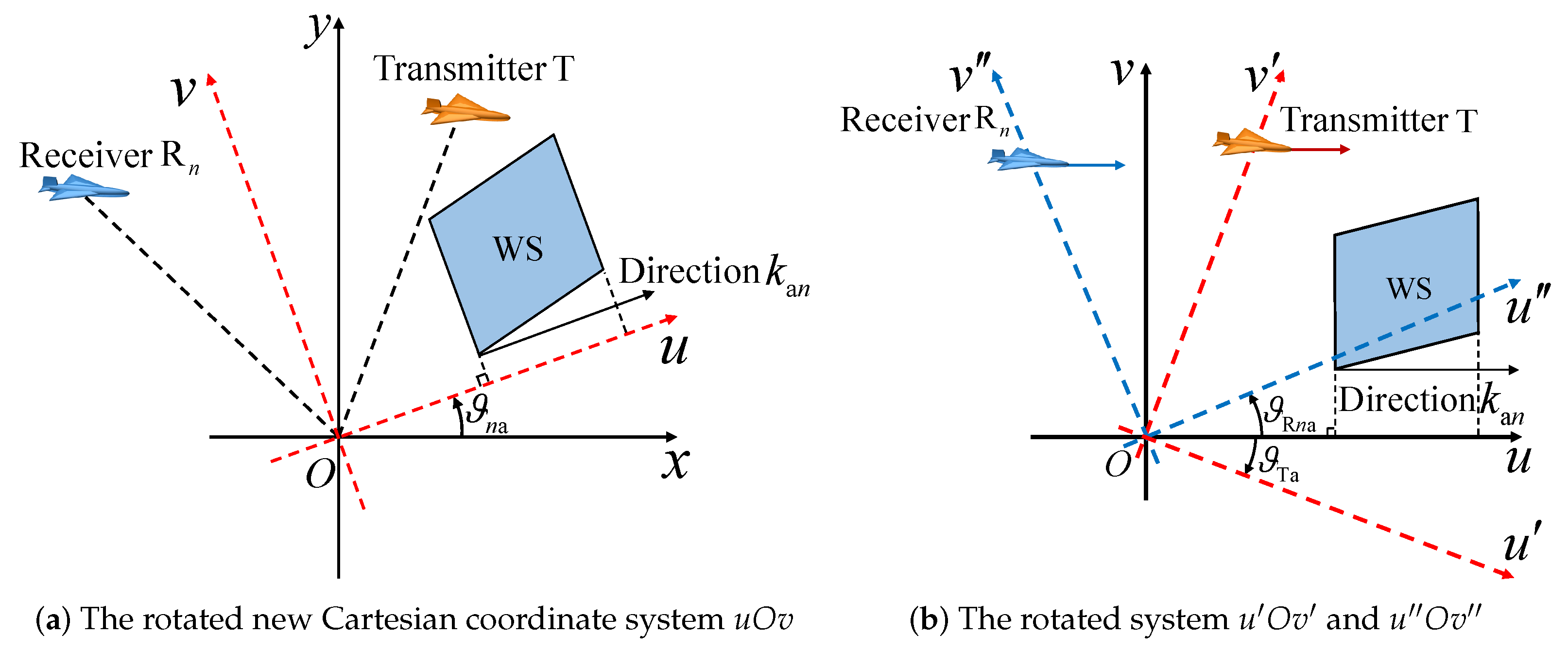
3.1. The Distribution Principles of WS

Similarly, taking the origin point O as the reference point, whose instantaneous range history is $R_{nO}\left(\tau \right)=R_{\mathrm{T}O}\left(\tau \right)+R_{\mathrm{R}nO}\left(\tau \right)$. By correlating the echoes of P and O, the range frequency domain expression of the echo from target point P can be written as

$$\begin{array}{c}{S}_n\left(f_t,\tau \right)=A·\mathrm{rect}\left(\frac{\tau }{T_a}\right)·\mathrm{rect}\left[\frac{f_t}{K_r{T}_r}\right]·exp\left\{j\frac{2\pi }{c}\left(f_c+f_t\right)\left[R_{nP}\left(\tau \right)-R_{nO}\left(\tau \right)\right]\right\}\hfill \end{array}$$

(3)

According to the far-field approximation, the range history difference between target points P and O can be approximated as follows:

$$\begin{array}{c}{R}_{nP}\left(\tau \right)-R_{nO}\left(\tau \right)=\left|R_{\mathrm{T}P}\left(\tau \right)+R_{\mathrm{R}nP}\left(\tau \right)\right|-\left|R_{\mathrm{T}O}\left(\tau \right)+R_{\mathrm{R}nO}\left(\tau \right)\right|\hfill \\ \approx x\left[cos{\alpha }_{\mathrm{T}}\left(\tau \right)cos{\theta }_{\mathrm{T}}\left(\tau \right)+cos{\alpha }_{\mathrm{R}n}\left(\tau \right)cos{\theta }_{\mathrm{R}n}\left(\tau \right)\right]\hfill \\ +y\left[cos{\alpha }_{\mathrm{T}}\left(\tau \right)sin{\theta }_{\mathrm{T}}\left(\tau \right)+cos{\alpha }_{\mathrm{R}n}\left(\tau \right)sin{\theta }_{\mathrm{R}n}\left(\tau \right)\right]\hfill \end{array}$$

(4)

Select the transmitter and the $n\mathrm{th}$ receiver for further analysis, and define the WS variables in the x and y directions as follows:

$$\left\{\begin{array}{c}{k}_{xn}\left(f_t,\tau \right)=k_{fn}\left[cos{\alpha }_{\mathrm{T}}\left(\tau \right)cos{\theta }_{\mathrm{T}}\left(\tau \right)+cos{\alpha }_{\mathrm{R}n}\left(\tau \right)cos{\theta }_{\mathrm{R}n}\left(\tau \right)\right]\hfill \\ k_{yn}\left(f_t,\tau \right)=k_{fn}\left[cos{\alpha }_{\mathrm{T}}\left(\tau \right)sin{\theta }_{\mathrm{T}}\left(\tau \right)+cos{\alpha }_{\mathrm{R}n}\left(\tau \right)sin{\theta }_{\mathrm{R}n}\left(\tau \right)\right]\hfill \end{array}\right.$$

(5)

where $k_{fn}=2\pi \left(f_{cn}+f_t\right)/c$ represents the spatial frequency of the transmitted signal. It can be concluded from (5) that the WS variable $\left[k_{xn}\left(f_t,\tau \right),k_{yn}\left(f_t,\tau \right)\right]$ is only determined by the frequency of the signal and the spatial position of the radar platforms. Then, the wavenumber domain expression of the echo can be written as

$$s_n\left(k_{xn},k_{yn}\right)=A_n·exp\left[j\left(x{k}_{xn}+y{k}_{yn}\right)\right]$$

(6)

where $s_n\left(k_{xn},k_{yn}\right)$ is called the wavenumber spectrum (WS) and $A_n$ expresses the normalized amplitude of the WS. As shown in Figure 2, under the condition of far-field approximation, the coverage of WS formed by a transmitter and the $n\mathrm{th}$ receiver is approximately a parallelogram region ${\Omega }_n$. In Figure 2, $B_{\mathrm{a}}$ and $B_f$ express the projection bandwidth of WS in directions ${\mathrm{k}}_{\mathrm{a}}$ and ${\mathrm{k}}_f$, respectively, and they will determine the resolution of the reconstructed point spread function (PSF) in these two directions [10,44,45].

The echoes of all receivers in MuA-SAR system are coherently projected into wavenumber domain, and the fused WS can be expressed as

$$s\left(k_x,k_y\right)=\sum _{n=1}^N{A}_n^{{}^{\prime }}·\sum _{\left[k_{xn}\left(f_t,\tau \right),k_{yn}\left(f_t,\tau \right)\right]\in \Omega n}^{}\left[k_{xn}\left(f_t,\tau \right),k_{yn}\left(f_t,\tau \right)\right]$$

(7)

where $A_n^{{}^{\prime }}$ is the normalized amplitude of WS of the $n\mathrm{th}$ receiver. Finally, the relationship between the WS of MuA-SAR system and PSF can be expressed by matrix Fourier transform (MFT) as

$$\sigma \left(x,y\right)=\underset{\left(k_x,k_y\right)\in \Omega }{\int \int }s\left(k_x,k_y\right)·e^{-j\left(x{k}_x+y{k}_y\right)}d{k}_{x}d{k}_y$$

(8)

where $\sigma \left(x,y\right)$ denotes the scattering coefficient of target point. $\Omega$ represents the effective coverage of all the WS region of MuA-SAR system.

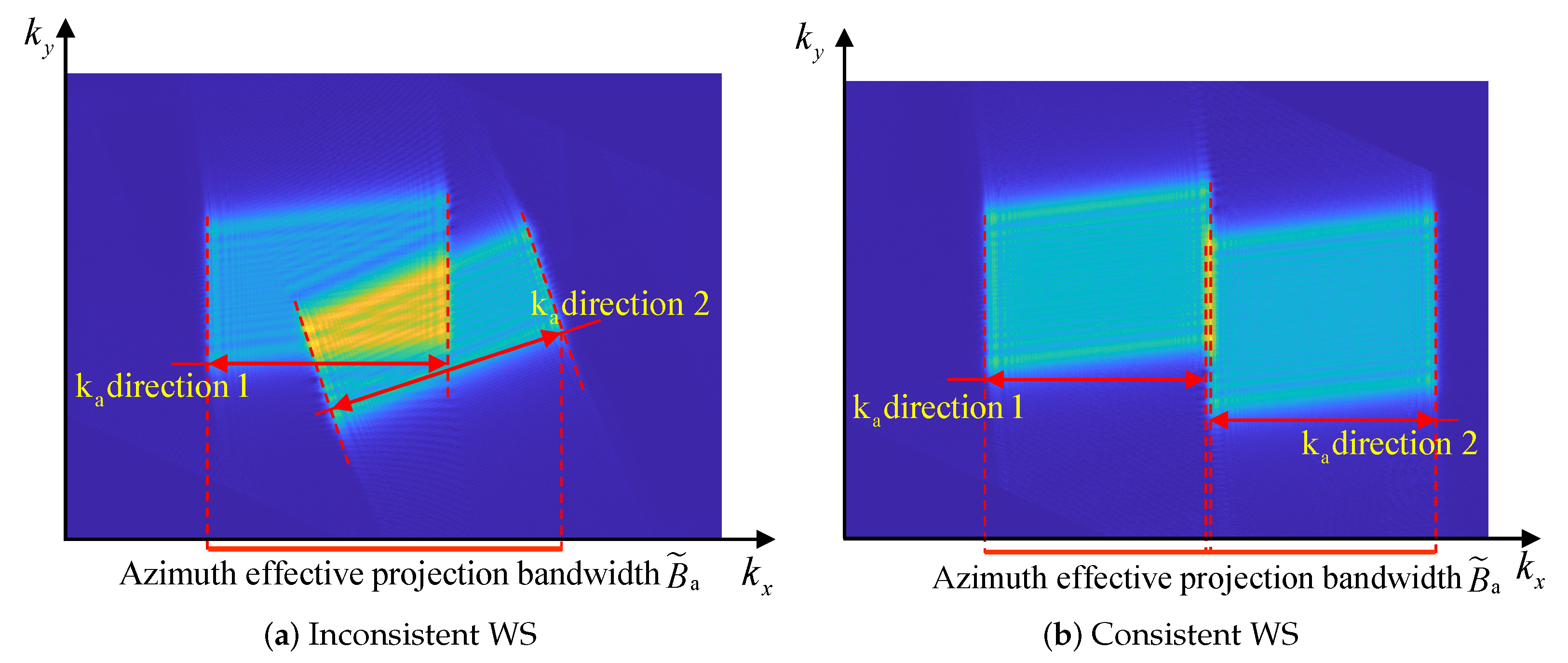
3.2. Influence of Consistency of WS Distribution on Imaging

Since the range resolution can be achieved by transmitting wideband signals, only the improvement in azimuth resolution will be analyzed in this paper. From (5), it can be seen that the distribution of WS is influenced by both the spatial configuration of the radar platforms and the signal parameters. In the MuA-SAR system, different radar platforms are completely separated in space, and their WS extension directions are also inconsistent. Taking a MuA-SAR system consisting of one transmitter and two receivers for imaging the origin point target as an example, Figure 3 shows the two distribution states of WS and the measurement method of effective projection bandwidth. In Figure 3a, the two WS are distributed in different extension directions, while in Figure 3b, the WS of one receiver is aligned with the ${\mathrm{k}}_{\mathrm{a}}$ direction of another one through rotation mapping. According to the relationship between WS and reconstructed PSF in (8), the resolution of the reconstructed PSF in the two directions can be expressed as

$$\left\{\begin{array}{c}{\rho }_{\mathrm{a}}=2\pi /B_{\mathrm{a}n}\hfill \\ {\rho }_f=2\pi /B_{fn}\hfill \end{array}\right.$$

(9)

where $B_{\mathrm{a}n}$ and $B_{fn}$, respectively, represent the equivalent WS projection bandwidth of the MuA-SAR system in ${\mathrm{k}}_{\mathrm{a}}$ and ${\mathrm{k}}_f$ directions. Based on Figure 3, it can be seen that if the WS of each bistatic radar pair in the MuA-SAR system is rotated and aligned in the ${\mathrm{k}}_{\mathrm{a}}$ direction, a larger equivalent projection bandwidth in the azimuth direction can be obtained, thereby fully utilizing the azimuth echo data.

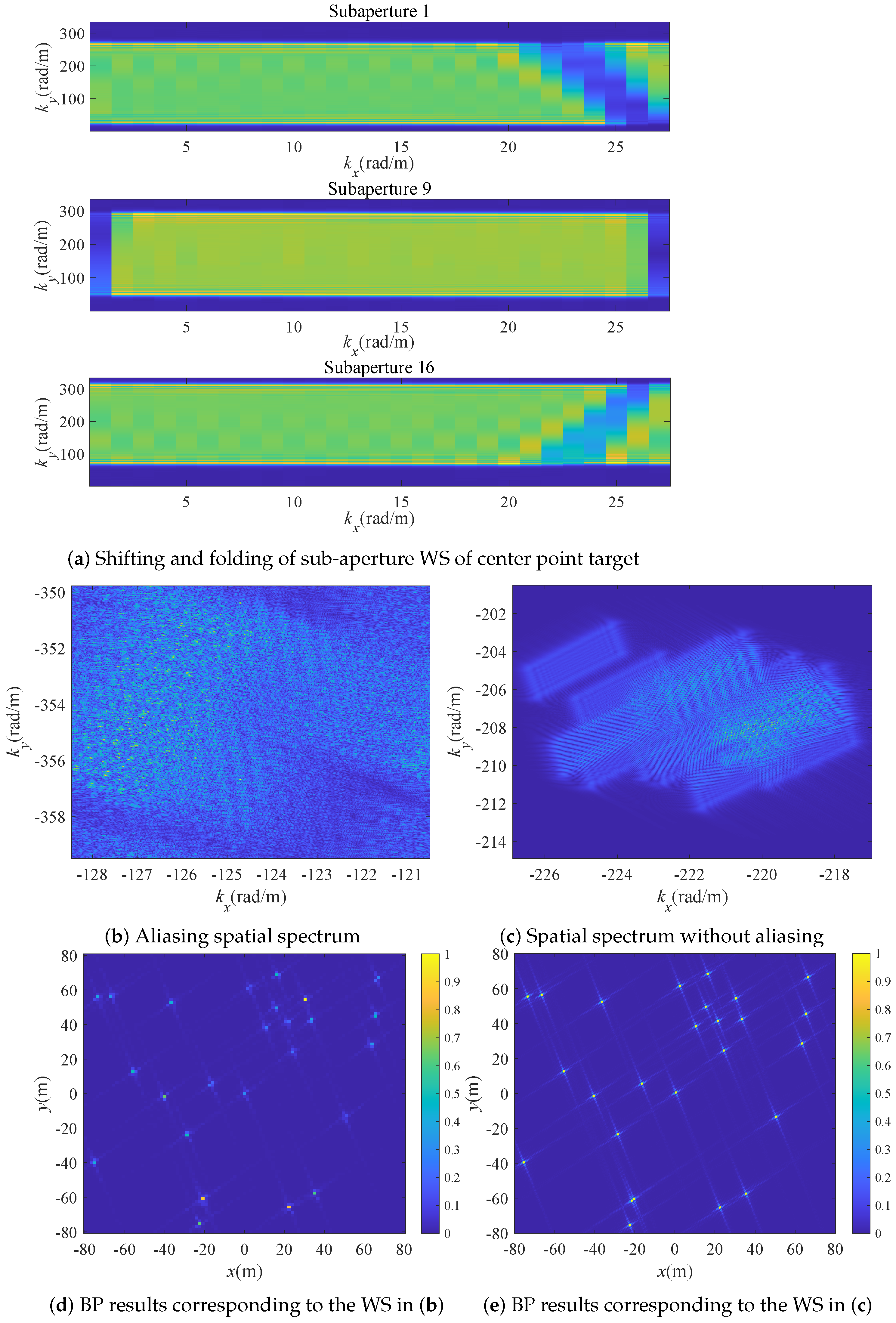
3.3. Analysis of Aliasing Phenomenon of WS

Take a pair of bistatic radars as an example to analyze. Projection of the range frequency domain expression of the echo in (3) to the wavenumber domain, and the wavenumber domain expression of any point $P_i\left(x_i,y_i,0\right)$ in the scene can be expressed as

$$S_{n{P}_i}\left(f_t,\tau \right)=A_n\left(\tau \right)·{\sigma }_{P_i}·\mathrm{rect}\left(\frac{\tau }{T_a}\right)·\mathrm{rect}\left(\frac{k-k_{cn}}{k_{Bn}}\right)·exp\left[-j{k}_{fn}{R}_{n{P}_i}\left(\tau \right)\right]$$

(10)

where ${\sigma }_{P_i}$ is the scattering coefficient of point $P_i$. $k_{cn}=2\pi f_{cn}/c$ and $k_{Bn}=2\pi B_{fn}/c$ represent the center and the range bandwidth of the wavenumber of the bistatic radar pair, respectively. Therefore, the wavenumber domain echo expression of the imaging scene can be expressed as the superposition of all the point target echoes in the scene, that is

$$S_n\left(f_t,\tau \right)=\sum _{P_i\in \Omega }{S}_{n{P}_i}\left(f_t,\tau \right)$$

(11)

By compensating the phase of echo in wavenumber domain, the back projection of point target can be realized, and the reconstructed result of point target can be expressed as

$$I_n\left(x_i,y_i\right)={\int }_0^{T_a}{\int }_{2\pi \left(f_{cn}-\frac{B_{fn}}{2}\right)/c}^{2\pi \left(f_{cn}+\frac{B_{fn}}{2}\right)/c}{S}_n\left(f_t,\tau \right)·exp\left[-j{k}_{fn}{R}_{n{P}_i}\left(\tau \right)\right]d{f}_{t}d\tau$$

(12)

where $R_{n{P}_i}\left(\tau \right)$ represents the instantaneous range history of bistatic radar pair relative to point target $P_i$, i.e.,

$$\begin{array}{c}{R}_{n{P}_i}\left(\tau \right)=R_{\mathrm{T}{P}_i}\left(\tau \right)+R_{\mathrm{R}n{P}_i}\left(\tau \right)\hfill \\ =\sqrt{{\left[x_{\mathrm{T}}\left(\tau \right)-x_i\right]}^2+{\left[y_{\mathrm{T}}\left(\tau \right)-y_i\right]}^2+z_{\mathrm{T}}^2\left(\tau \right)}+\sqrt{{\left[x_{\mathrm{R}n}\left(\tau \right)-x_i\right]}^2+{\left[y_{\mathrm{R}n}\left(\tau \right)-y_i\right]}^2+z_{\mathrm{R}n}^2\left(\tau \right)}\hfill \end{array}$$

(13)

The expression of the WS of the reconstructed result in (12) can be obtained by two-dimensional inverse Fourier transform (2D IFFT), that is

$$I_n\left(k_{xn},k_{yn}\right)={\int }_{-\infty }^{+\infty }{\int }_{-\infty }^{+\infty }{I}_n\left(x_i,y_i\right)·exp\left[-j\left(k_{xn}{x}_i+k_{yn}{y}_i\right)\right]d{x}_{i}d{y}_i$$

(14)

where $\left(k_{xn},k_{yn}\right)$ represents the wavenumber coordinates in GCCS corresponding to the imaging results of the bistatic radar pair. Using the principle of stationary phase (POSP) to calculate the integral Expression (14), the coordinates of the stationary phase point can be calculated by taking partial derivatives of $x_i$ and $y_i$ with the phase part, that is

$$\left\{\begin{array}{c}\frac{\partial }{\partial x_i}\left[k_{fn}{R}_{n{P}_i}\left(\tau \right)-k_{xn}{x}_i\right]=0\hfill \\ \frac{\partial }{\partial y_i}\left[k_{fn}{R}_{n{P}_i}\left(\tau \right)-k_{yn}{y}_i\right]=0\hfill \end{array}\right.\Rightarrow \left\{\begin{array}{c}{k}_{xn}=k_{fn}·\left[\frac{x_i-x_{\mathrm{T}}\left(\tau \right)}{R_{\mathrm{T}{P}_i}\left(\tau \right)}+\frac{x_i-x_{\mathrm{R}n}\left(\tau \right)}{R_{\mathrm{R}n{P}_i}\left(\tau \right)}\right]\hfill \\ k_{yn}=k_{fn}·\left[\frac{y_i-y_{\mathrm{T}}\left(\tau \right)}{R_{\mathrm{T}{P}_i}\left(\tau \right)}+\frac{y_i-y_{\mathrm{R}n}\left(\tau \right)}{R_{\mathrm{R}n{P}_i}\left(\tau \right)}\right]\hfill \end{array}\right.$$

(15)

The value range of point $\left(k_{xn},k_{yn}\right)$ in the wavenumber domain is the distribution range of WS corresponding to the signal of this channel. Substituting the velocity components of the transmitter and the $n\mathrm{th}$ receiver in directions x and y, the $k_{xn}$ and $k_{yn}$ can be updated to

$$\left\{\begin{array}{c}{k}_{xn}=k_{fn}·\left[\frac{x_i-x_{\mathrm{T}}\left(\tau \right)\left|{}_{\tau =0}\right.-v_{\mathrm{T}x}\tau }{R_{\mathrm{T}{P}_i}\left(\tau \right)}+\frac{x_i-x_{\mathrm{R}n}\left(\tau \right)\left|{}_{\tau =0}\right.-v_{\mathrm{R}nx}\tau }{R_{\mathrm{R}n{P}_i}\left(\tau \right)}\right]\hfill \\ k_{yn}=k_{fn}·\left[\frac{y_i-y_{\mathrm{T}}\left(\tau \right)\left|{}_{\tau =0}\right.-v_{\mathrm{T}y}\tau }{R_{\mathrm{T}{P}_i}\left(\tau \right)}+\frac{y_i-y_{\mathrm{R}n}\left(\tau \right)\left|{}_{\tau =0}\right.-v_{\mathrm{R}ny}\tau }{R_{\mathrm{R}n{P}_i}\left(\tau \right)}\right]\hfill \end{array}\right.$$

(16)

It can be seen from (16) that the distribution range of WS of point target in wavenumber domain is determined by the following two aspects: On the one hand, the terms related to the velocity of radar platforms show that the width of the WS is affected by the aperture formed by the motion of radar platforms. On the other hand, the term related to the analyzed point target coordinates shows that the width of the WS is also affected by the width of the scene. Both of the above two aspects will lead to the degradation of the imaging quality of MuA-SAR system or even can not imaging.

Select a pair of bistatic radars and a set of typical parameters to analyze the shifting and folding of sub-aperture WS, as well as the aliasing phenomenon caused by WS broadening. Select the echo data of the scene center point and divide it into 16 sub-apertures. Then, process each sub-aperture data by BP algorithm and project the imaging results into the wavenumber domain by 2D-IFFT. The wavenumber spectra of the selected sub-aperture 1, 9 and 16 are shown in Figure 4a. It can be seen from Figure 4a that, due to the low resolution of the azimuth imaging grid division, the corresponding wavenumber domain range is narrow. It causes the WS of the same point target to shift and fold. Figure 4b shows the WS distribution when the grid division resolution is close to the theoretical resolution calculated by (9), and it can be seen that WS of different scattering points exists serious aliasing phenomenon; Figure 4c shows the WS distribution when the grid division resolution is much higher than the theoretical resolution, and the WS of different point targets can be distinguished without aliasing. Figure 4d is the BP imaging results of randomly distributed point targets corresponding to the WS in Figure 4b, and the imaging quality is seriously degraded, and even some targets are lost. Figure 4e is the BP imaging results of randomly distributed point targets corresponding to the WS in Figure 4c, and it has good imaging quality.

According to the above analysis, to obtain high-resolution imaging results efficiently by using the BP-based method, it is necessary to divide the imaging grid reasonably according to the WS distribution and avoid the folding of WS while making full use of the echo data. Additionally, it is necessary to compress the through phase compensation to avoid WS aliasing. In the next section, a fast imaging algorithm based on FFBP algorithm architecture is proposed, which can ensure the accuracy and quality of imaging at the same time.

4. Proposed Algorithm

In this section, a UCFFBP algorithm with multi-level regional attention strategy for MuA-SAR fast imaging is proposed. First, the steps of the imaging algorithm are introduced. Then, the computational complexity of the proposed algorithm is analyzed in detail.

4.1. Description of the Proposed Algorithm

The flowchart of the imaging algorithm is shown in Figure 5, in which the red-dotted box illustrates the coherent fusion imaging process based on multi-level regional attention strategy, and the flow chart of this process is shown in the right part of Figure 5.

Taking the bistatic radar pair composed of the transmitter and the $n\mathrm{th}$ receiver as an example, the algorithm steps are described below, which can be mainly divided into four main steps:

Step (1) Establishment of GCCS and rotate the coordinate system to align WS in azimuth:

First, establish the GCCS $xOy$. Then, according to the analysis in Section 3.2, to make full use of the azimuth sampling data at the initial level of BP imaging processing, it is necessary to rotate the coordinate system to align WS in the selected azimuth. As shown in Figure 6a, assuming that the new Cartesian coordinate system after rotation is $uOv$, the coordinates of the transmitter and receiver after rotation mapping can be expressed as

$$\left\{\begin{array}{c}\left(u_{\mathrm{T}},v_{\mathrm{T}}\right)=\left(x_{\mathrm{T}},y_{\mathrm{T}}\right){\mathbf{r}}_{\vartheta n\mathrm{a}}\hfill \\ \left(u_{\mathrm{R}n},v_{\mathrm{R}n}\right)=\left(x_{\mathrm{R}n},y_{\mathrm{R}n}\right){\mathbf{r}}_{\vartheta n\mathrm{a}}\hfill \end{array}\right.$$

(17)

where ${\mathbf{r}}_{\vartheta n\mathrm{a}}$ represents a rotation mapping matrix, which can be specifically expressed as

$${\mathbf{r}}_{\vartheta n\mathrm{a}}=\left[\begin{array}{cc}cos{\vartheta }_{n\mathrm{a}}& sin{\vartheta }_{n\mathrm{a}}\\ -sin{\vartheta }_{n\mathrm{a}}& cos{\vartheta }_{n\mathrm{a}}\end{array}\right]$$

(18)

where ${\vartheta }_{n\mathrm{a}}$ indicates the counterclockwise rotation angle required to align with ${\mathrm{k}}_{\mathrm{a}}$ direction of the WS of the $n\mathrm{th}$ bistatic radar pair.

Because the platforms in the MuA-SAR system are independent of each other, to facilitate the subsequent phase compensation processing, it is necessary to divide the design of the rotation mapping matrix into transmitter and receiver separately. As shown in Figure 6b, the direction $Ou$ in the coordinate system $uOv$ is the direction that the WS azimuth extension direction of the bistatic radar pair needs to rotate and align. Then, the transmitter’s local coordinate system $u^{\prime }O{v}^{\prime }$ and the receiver’s local coordinate system $u^{″}O{v}^{″}$ are established with the full aperture centers of the transmitter and $n\mathrm{th}$ receiver as the origin and the azimuth direction of the radar platform as the ordinate, respectively. In Figure 6b, ${\vartheta }_{\mathrm{Ta}}$ and ${\vartheta }_{\mathrm{R}n\mathrm{a}}$, respectively, indicate that the rotation angles of coordinate systems $u^{\prime }O{v}^{\prime }$ and $u^{″}O{v}^{″}$ are needed to align with the coordinate system $uOv$.

At this time, in the transmitter’s local coordinate system $u^{\prime }O{v}^{\prime }$, the coordinates of the transmitter and the grid points are as follows:

$$\left\{\begin{array}{c}\left({u^{\prime }}_{\mathrm{T}},{v^{\prime }}_{\mathrm{T}}\right)=\left(u_{\mathrm{T}},v_{\mathrm{T}}\right){\mathbf{r}}_{\mathrm{Ta}}\hfill \\ \left({u^{\prime }}_i,{v^{\prime }}_i\right)=\left(u_i,v_i\right){\mathbf{r}}_{\mathrm{Ta}}\hfill \end{array}\right.$$

(19)

In (19), the rotation mapping matrix is constructed according to the transmitter’s local coordinate system, and its specific expression is

$${\mathbf{r}}_{\mathrm{Ta}}=\left[\begin{array}{cc}cos{\vartheta }_{\mathrm{Ta}}& sin{\vartheta }_{\mathrm{Ta}}\\ -sin{\vartheta }_{\mathrm{Ta}}& cos{\vartheta }_{\mathrm{Ta}}\end{array}\right]$$

(20)

where ${\vartheta }_{\mathrm{Ta}}$ is the angle required for clockwise rotation of the transmitter local coordinate system $u^{\prime }O{v}^{\prime }$ to align with the coordinate system $uOv$. In the receiver’s local coordinate system $u^{″}O{v}^{″}$, the coordinates of the transmitter and the grid points are as follows:

$$\left\{\begin{array}{c}\left({u^{″}}_{\mathrm{R}n\mathrm{a}},{v^{″}}_{\mathrm{R}n\mathrm{a}}\right)=\left(u_{\mathrm{R}n\mathrm{a}},v_{\mathrm{R}n\mathrm{a}}\right){\mathbf{r}}_{\mathrm{R}n\mathrm{a}}\hfill \\ \left({u^{″}}_i,{v^{″}}_i\right)=\left(u_i,v_i\right){\mathbf{r}}_{\mathrm{R}n\mathrm{a}}\hfill \end{array}\right.$$

(21)

In (21), the rotation mapping matrix is constructed according to the receiver’s local coordinate system, and its specific expression is

$${\mathbf{r}}_{\mathrm{R}n\mathrm{a}}=\left[\begin{array}{cc}cos{\vartheta }_{\mathrm{R}n\mathrm{a}}& sin{\vartheta }_{\mathrm{R}n\mathrm{a}}\\ -sin{\vartheta }_{\mathrm{R}n\mathrm{a}}& cos{\vartheta }_{\mathrm{R}n\mathrm{a}}\end{array}\right]$$

(22)

where ${\vartheta }_{\mathrm{R}n\mathrm{a}}$ is the angle required for clockwise rotation of the receiver’s local coordinate system $u^{″}O{v}^{″}$ to align with the coordinate system $uOv$.

Step (2) Sub-aperture division and low-resolution grid division at initial level:

After the azimuthal alignment of WS is completed, the azimuthal WS is utilized to the maximum extent. At this time, the projection grid can be divided with the lowest resolution as possible under the condition of ensuring the coherence of signals, and the imaging efficiency is improved. In this imaging algorithm, the final imaging result is obtained through level-by-level recursive fusion of the initial level BP imaging results. Therefore, the resolution of the initial grid division will be much lower than the final imaging resolution of the system. However, according to the analysis in Section 3.2, a grid division of too low a resolution will lead to WS aliasing of sub-aperture data, so it is necessary to set a reasonable initial back projection grid division width according to the length of sub-aperture division and the WS distribution range after rotation alignment.

First, according to the requirements of imaging accuracy and efficiency, the echo data of each bistatic radar pair is divided into $K_{sub}^{\left(0\right)}=2^G$ at the initial level, and then the distribution range of WS is calculated according to the spatial configuration parameters of bistatic radar pair after rotation and alignment. Assume that the WS distribution range of the first bistatic radar pair after rotation and alignment are as follows:

$$\left\{\begin{array}{c}{k}_{un}\left(f_t,\tau \right)\in \left[k_{un}^{min}\left(f_t,\tau \right),k_{un}^{max}\left(f_t,\tau \right)\right]\hfill \\ k_{vn}\left(f_t,\tau \right)\in \left[k_{vn}^{min}\left(f_t,\tau \right),k_{vn}^{max}\left(f_t,\tau \right)\right]\hfill \end{array}\right.$$

(23)

where $k_{un}\left(f_t,\tau \right)$ and $k_{vn}\left(f_t,\tau \right)$ represent the coordinates of the WS sampling points in the u and v directions after rotation mapping.

Second, because the data of different bistatic radar pairs need to be back-projected into the same Cartesian coordinate system in the following steps, it needs to be comprehensively determined by the distribution range of all bistatic radar pairs when calculating the grid division width. The width of the grid in the u and v directions can be divided as follows:

$$\left\{\begin{array}{c}du=2\pi /\left|\underset{n=1,2,\dots ,N}{max}\left[k_{un}^{max}\left(f_t,\tau \right)\right]-\underset{n=1,2,\dots ,N}{min}\left[k_{un}^{min}\left(f_t,\tau \right)\right]\right|\hfill \\ dv=2\pi /\left|\underset{n=1,2,\dots ,N}{max}\left[k_{vn}^{max}\left(f_t,\tau \right)\right]-\underset{n=1,2,\dots ,N}{min}\left[k_{vn}^{min}\left(f_t,\tau \right)\right]\right|\hfill \end{array}\right.$$

(24)

Step (3) BP of sub-aperture data at initial level:

The sub-aperture data of each bistatic radar are back projected to GCCS one by one and imaged separately. The $k\mathrm{th}\left(k=1,2,\dots ,K_{sub}^{\left(0\right)}\right)$ sub-aperture back projection imaging result obtained by the $n\mathrm{th}\left(n=1,2,\dots ,N\right)$ bistatic radar pair at the initial level $\left(g=0\right)$ can be expressed as

$$I_{\left(n,k\right)}\left(u_i,v_i\right)={\int }_{\left[\left(k-1\right)·T_a\right]/K_{sub}^{\left(0\right)}}^{\left(k·T_a\right)/K_{sub}^{\left(0\right)}}{\int }_{2\pi \left(f_{cn}-\frac{B_{fn}}{2}\right)/c}^{2\pi \left(f_{cn}+\frac{B_{fn}}{2}\right)/c}{S}_n\left(f_t,\tau \right)·exp\left[-j{k}_{f\left(n,k\right)}{R}_{n{P}_i}\left(\tau \right)\right]d{f}_{t}d\tau$$

(25)

Transform the above imaging results into wavenumber domain, that is

$$I_{\left(n,k\right)}\left(k_u,k_v\right)={\int }_{-\infty }^{+\infty }{\int }_{-\infty }^{+\infty }{I}_{\left(n,k\right)}\left(u_i,v_i\right)·exp\left[-j\left(k_{un}{u}_i+k_{vn}{v}_i\right)\right]d{u}_{i}d{v}_i$$

(26)

where $\left(k_u,k_v\right)$ is the coordinate of the WS in the coordinate system $uOv$.

Step (4) Multi-level regional attention strategy and phase compensation of sub-images:

This step can be divided into two aspects: multi-level regional attention strategy and second-order phase compensation. For the multi-level regional attention strategy, normally, there are some differences between the gray values of the target and the background region in SAR images. The gray values of the target region are stably distributed in the high range, while the background region usually contains noise and clutter, and its gray values are usually unstably distributed in the lower range. Therefore, it can be considered that the target region satisfies the condition of the MSER, which makes the algorithm pay more attention to the MSER at each fusion level in the fusion process [46,47,48]. As shown in Figure 7, SAR imaging of a ship on the sea is analyzed as an example to introduce the specific steps.

First, for the sub-image obtained at a certain fusion level, the distribution range of its gray value is measured, and M equally spaced threshold values $\Delta h$ are set in this gray value distribution range. Two adjacent threshold values satisfy the following relationship

$$h_{m+1}=h_m+\Delta h,m=1,2,\dots ,M-1$$

(27)

Then, based on each threshold, the image is binarized, that is, the pixels with gray values below the threshold are set to 0, and the pixels with gray values above the threshold are set to 1. At this time, M binary images can be obtained. In each binary image, the region with a gray value of 1 is called the extremal region, and the extremal regions divided by different thresholds satisfy $A_{hM}\subset A_{hM-1}\subset ,\dots ,\subset A_{h1}$.

In the imaging results obtained at each fusion level, the target area is usually bright, which is in great contrast with the background area, and the gray level of the target area will remain stable in a certain range. According to this characteristic, the change rate of the areas of two adjacent extremal regions is counted and the areas with stable gray levels in a certain range are selected as suspected target regions according to the following criteria:

$${\eta }_m=\frac{\left|S\left(A_{hm+1}\right)-S\left(A_{hm}\right)\right|}{S\left(A_{hm}\right)}<\mu ,m=1,2,\dots ,M$$

(28)

where $S\left(·\right)$ represents the area of extremal regions, ${\eta }_m$ represents the change rate of the extremal region area when the threshold value is $h_m$, and $\mu$ represents the maximum value of the change rate of the extremal region area. At the $g\mathrm{th}\left(g=0,1,\dots ,G-1\right)$ fusion level, the number of sub-images included is $k_n^{\left(g\right)}=2^{G-g}$. Because the difference between sub-images corresponding to adjacent sub-apertures is small, to further reduce redundant calculation, only $G-g$ sub-images need to be selected at intervals from all sub-images for image segmentation at each fusion level. Then, the coordinates and gray values of the segmented pixels are transferred to the next level for fusion. Specifically, firstly, all the sub-images obtained at each fusion level are numbered according to the time sequence of acquisition; secondly, the sub-images numbered $\mathrm{ROUND}\left[2^{G-g}/\left(G-g\right)·n_g\right],n_g=1,2,\dots ,G-g$ are selected for segmentation, where $\mathrm{ROUND}\left[·\right]$ expresses rounding operation. The extremal regions segmented in the selected sub-images are denoted as $A_i^{\left(g\right)}\left(i=1,2,\dots G-g\right)$. To ensure the accuracy of the final imaging result, the pixel points that have appeared in each extreme value area are merged to obtain a pixel point set and transmitted to the next fusion level, that is,

$$A^{\left(g\right)}=\bigcup A_i^{\left(g\right)},i=1,2,\dots G-g$$

(29)

Then, suppose that the merged pixel set $A^{\left(g\right)}$ contains $K_i$ pixels, and each pixel can be expressed as $p_{ki}\left(x_{ki},y_{ki}\right),k_i=1,2,\dots ,K_i$, where $\left(x_{ki},y_{ki}\right)$ represents the coordinates of pixel $p_{ki}$. Count the number of times each pixel appears according to the following criteria:

$$c_{ki}=\left\{\begin{array}{c}1,p_{ki}\left(x_{ki},y_{ki}\right)\in A_i^{\left(g\right)},i=1,2,\dots \hfill \\ 0,p_{ki}\left(x_{ki},y_{ki}\right)\notin A_i^{\left(g\right)},i=1,2,\dots \hfill \end{array}\right.$$

(30)

$$N_{pk}=\sum _{i=1}^{G-g}{c}_{ki}$$

(31)

The empirical threshold $\widehat{N}$ is set to determine whether to keep the pixel, that is, when $N_{pk}⩾\widehat{N}$, the pixel is kept. Otherwise, the gray value of the pixel is set to zero. Finally, after traversing all the pixels in the set $A^{\left(g\right)}$, the pixels whose gray value is not 0 are transferred to the next fusion level.

For the second-order phase compensation, it needs to be carried out in each sub-image at each recursive fusion level. Here, the $k\mathrm{th}\left(k=1,2,\dots ,K_{sub}^{\left(g\right)}\right)$ sub-aperture of the $n\mathrm{th}\left(n=1,2,\dots ,N\right)$ bistatic radar pair at the $g\mathrm{th}\left(g=0,1,\dots ,G-1\right)$ fusion level is taken as an example for analysis. $K_{sub}^{\left(g\right)}=2^{G-g}$ is the total number of equivalent sub-apertures at the current fusion level.

First, according to the POSP, the stationary phase point equations of this sub-aperture can be constructed and solved as follows:

$$\left\{\begin{array}{c}\frac{\partial }{\partial u_i}\left[k_{f\left(n,k\right)}{R}_{n{P}_i}\left(\tau \right)-k_{u\left(n,k\right)}{u}_i\right]=0\hfill \\ \frac{\partial }{\partial v_i}\left[k_{f\left(n,k\right)}{R}_{n{P}_i}\left(\tau \right)-k_{v\left(n,k\right)}{v}_i\right]=0\hfill \end{array}\right.\Rightarrow \left\{\begin{array}{c}{k}_{u\left(n,k\right)}=k_{f\left(n,k\right)}·\left[\frac{u_i-u_{\mathrm{T}}\left(\tau \right)}{R_{\mathrm{T}{P}_i}\left(\tau \right)}+\frac{u_i-u_{\mathrm{R}n}\left(\tau \right)}{R_{\mathrm{R}n{P}_i}\left(\tau \right)}\right]\hfill \\ k_{v\left(n,k\right)}=k_{f\left(n,k\right)}·\left[\frac{v_i-v_{\mathrm{T}}\left(\tau \right)}{R_{\mathrm{T}{P}_i}\left(\tau \right)}+\frac{v_i-v_{\mathrm{R}n}\left(\tau \right)}{R_{\mathrm{R}n{P}_i}\left(\tau \right)}\right]\hfill \end{array}\right.$$

(32)

where $R_{n{P}_i}\left(\tau \right)$ is the instantaneous range history in the coordinate system $uOv$, and its specific expression is

$$\begin{array}{c}{R}_{n{P}_i}\left(\tau \right)=R_{\mathrm{T}{P}_i}\left(\tau \right)+R_{\mathrm{R}n{P}_i}\left(\tau \right)\hfill \\ =\sqrt{{\left[u_{\mathrm{T}}\left(\tau \right)-u_i\right]}^2+{\left[v_{\mathrm{T}}\left(\tau \right)-v_i\right]}^2+z_{\mathrm{T}}^2\left(\tau \right)}+\sqrt{{\left[u_{\mathrm{R}n}\left(\tau \right)-u_i\right]}^2+{\left[v_{\mathrm{R}n}\left(\tau \right)-v_i\right]}^2+z_{\mathrm{R}n}^2\left(\tau \right)}\hfill \end{array}$$

(33)

where $R_{\mathrm{T}{P}_i}\left(\tau \right)$ and $R_{\mathrm{R}n{P}_i}\left(\tau \right)$ represent the instantaneous distances from the imaging grid point $P_i$ at the current fusion level to the transmitter and receiver, respectively. Combined with the analysis in Section 3.2, the aliasing phenomenon caused by the motion of the radar platform can be avoided by setting an appropriate grid division width at the initial level. According to (32), it is necessary to compensate the terms related to $u_i$ and $v_i$ to realize the compression of WS, and then solve the problem of WS aliasing.

Then, the influence of $u_i$ and $v_i$ on the WS can be divided into two aspects: the influence on the WS of the transmitter and receiver. According to (19), the WS components of the transmitter after rotation mapping in the transmitter’s local coordinate system $u^{\prime }O{v}^{\prime }$ can be obtained as follows:

$$\left\{\begin{array}{c}k{{}^{\prime }}_{u\left(n,k\right)}^{\mathrm{T}}=k_{f\left(n,k\right)}·\left[\frac{{u^{\prime }}_i-{u^{\prime }}_{\mathrm{T}}\left(\tau \right)}{{R^{\prime }}_{\mathrm{T}{P}_i}\left(\tau \right)}\right]\hfill \\ k{{}^{\prime }}_{v\left(n,k\right)}^{\mathrm{T}}=k_{f\left(n,k\right)}·\left[\frac{{v^{\prime }}_i-{v^{\prime }}_{\mathrm{T}}\left(\tau \right)}{{R^{\prime }}_{\mathrm{T}{P}_i}\left(\tau \right)}\right]\hfill \end{array}\right.$$

(34)

where $R_{\mathrm{T}{P}_i}^{\prime }\left(\tau \right)$ represents the instantaneous distance between $P_i\left({u^{\prime }}_i,{v^{\prime }}_i\right)$ and the transmitter in the transmitter’s local coordinate system, and its specific expression is

$$R_{\mathrm{T}{P}_i}^{\prime }\left(\tau \right)=\sqrt{{\left[{u^{\prime }}_{\mathrm{T}}\left(\tau \right)-{u^{\prime }}_i\right]}^2+{\left[{v^{\prime }}_{\mathrm{T}}\left(\tau \right)-{v^{\prime }}_i\right]}^2+z_{\mathrm{T}}^2\left(\tau \right)}$$

(35)

Assuming that ${\vartheta }_i^{\prime }\left(\tau \right)$ is the squint angle of the transmitter relative to the grid point in the transmitter’s local coordinate system, (34) can be written as

$$\left\{\begin{array}{c}k{{}^{\prime }}_{u\left(n,k\right)}^{\mathrm{T}}=k_{f\left(n,k\right)}·sin{{\vartheta }^{\prime }}_i\left(\tau \right)\hfill \\ k{{}^{\prime }}_{v\left(n,k\right)}^{\mathrm{T}}=k_{f\left(n,k\right)}·cos{{\vartheta }^{\prime }}_i\left(\tau \right)\hfill \end{array}\right.$$

(36)

Under far-field conditions, the scene width and synthetic aperture length are much smaller than the slope distance of the radar platforms, so it can be deduced that $sin{{\vartheta }^{\prime }}_i\left(\tau \right)\approx {{\vartheta }^{\prime }}_i\left(\tau \right)$ and $cos{{\vartheta }^{\prime }}_i\left(\tau \right)\approx 1$. Therefore, (36) can be approximately expressed as

$$\left\{\begin{array}{c}k{{}^{\prime }}_{u\left(n,k\right)}^{\mathrm{T}}\approx k_{f\left(n,k\right)}·{{\vartheta }^{\prime }}_i\left(\tau \right)\hfill \\ k{{}^{\prime }}_{v\left(n,k\right)}^{\mathrm{T}}\approx k_{f\left(n,k\right)}\hfill \end{array}\right.$$

(37)

It can be seen from (37) that the WS coordinate $k{{}^{\prime }}_{v\left(n,k\right)}^{\mathrm{T}}$ is only related to the frequency of the transmitted signal and is not affected by the distance between the point target and the center of the imaging scene. However, the coordinate $k{{}^{\prime }}_{u\left(n,k\right)}^{\mathrm{T}}$ is affected by both the aperture length of the transmitter and the width of the imaging scene. Further, expand (35) as follows:

$$R_{\mathrm{T}{P}_i}^{\prime }\left(\tau \right)=\sqrt{{\left[{u^{\prime }}_{\mathrm{T}}\left(\tau \right)\right]}^2-2{u^{\prime }}_{\mathrm{T}}\left(\tau \right){u^{\prime }}_i+u{{}^{\prime }}_i^2+{\left[{v^{\prime }}_{\mathrm{T}}\left(\tau \right)-{v^{\prime }}_i\right]}^2+z_{\mathrm{T}}^2\left(\tau \right)}$$

(38)

At the same time, by solving the stationary phase point equations in the transmitter’s local coordinate system of the current fusion level, one can obtain

$$\left\{\begin{array}{c}\frac{\partial }{\partial {u^{\prime }}_i}\left[k_{f\left(n,k\right)}{R^{\prime }}_{n{P}_i}\left(\tau \right)-k{{}^{\prime }}_{u\left(n,k\right)}^{\mathrm{T}}{u^{\prime }}_i\right]=0\hfill \\ \frac{\partial }{\partial {v^{\prime }}_i}\left[k_{f\left(n,k\right)}{R^{\prime }}_{n{P}_i}\left(\tau \right)-k{{}^{\prime }}_{v\left(n,k\right)}^{\mathrm{T}}{v^{\prime }}_i\right]=0\hfill \end{array}\right.\Rightarrow \left\{\begin{array}{c}k{{}^{\prime }}_{u\left(n,k\right)}^{\mathrm{T}}=k_{f\left(n,k\right)}\frac{{u^{\prime }}_i-{u^{\prime }}_{\mathrm{T}}\left(\tau \right)}{{R^{\prime }}_{n{P}_i}\left(\tau \right)}\hfill \\ k{{}^{\prime }}_{v\left(n,k\right)}^{\mathrm{T}}=k_{f\left(n,k\right)}\frac{{v^{\prime }}_i-{v^{\prime }}_{\mathrm{T}}\left(\tau \right)}{{R^{\prime }}_{n{P}_i}\left(\tau \right)}\hfill \end{array}\right.$$

(39)

It can be seen from (39) that when the point target deviates from the center of the scene, the reason why the WS is aliased is that the coordinate $k{{}^{\prime }}_{u\left(n,k\right)}^{\mathrm{T}}$ of the stationary phase point contains the term $u^{\prime }/R_{\mathrm{T}{P}_i}^{\prime }\left(\tau \right)$, which varies with the variable $u^{\prime }$. Therefore, if the second-order term $u^{\prime 2}$ about $u^{\prime }$ is compensated in (39), the WS can be compressed and aliasing can be avoided. The second-order phase compensation factor is constructed as follows. It is assumed that the (39) is updated as follows after phase compensation

$${\widetilde{R^{\prime }}}_{\mathrm{T}{P}_i}\left(\tau \right)=\sqrt{{\left[{u^{\prime }}_{\mathrm{T}}\left(\tau \right)\right]}^2-2{u^{\prime }}_{\mathrm{T}}\left(\tau \right){u^{\prime }}_i+{\left[{v^{\prime }}_{\mathrm{T}}\left(\tau \right)-{v^{\prime }}_i\right]}^2+z_{\mathrm{T}}^2\left(\tau \right)}$$

(40)

It can be deduced that

$$R_{\mathrm{T}{P}_i}^{\prime }\left(\tau \right)={\widetilde{R^{\prime }}}_{\mathrm{T}{P}_i}\left(\tau \right)+\sqrt{1+\frac{u{{}^{\prime }}_i^2}{{\left[{\widetilde{R^{\prime }}}_{\mathrm{T}{P}_i}\left(\tau \right)\right]}^2}}$$

(41)

Usually, because the distance from the transmitter to the grid point is much larger than the scene, that is $R_{\mathrm{T}{P}_i}^{\prime }\left(\tau \right)\gg u^{\prime }$, (41) can be expanded by the first-order Taylor and obtain [42]

$$R_{\mathrm{T}{P}_i}^{\prime }\left(\tau \right)\approx {\widetilde{R^{\prime }}}_{\mathrm{T}{P}_i}\left(\tau \right)+\frac{u{{}^{\prime }}_i^2}{2{\widetilde{R^{\prime }}}_{\mathrm{T}{P}_i}\left(\tau \right)}$$

(42)

Further, the wavenumber variable $k_{f\left(n,k\right)}$ is replaced by the center wavenumber $k_{c\left(n,k\right)}=2f_{c\left(n,k\right)}/c$ corresponding to the center frequency of the signal. Replace the slope distance of the whole sub-aperture with the slope distance corresponding to the current sub-aperture center time $\tau =\left(2k-1\right)T_a/2K_{sub}^{\left(g\right)}$. At this time, the second-order phase compensation factor in the transmitter’s local coordinate system can be approximately expressed as

$$H{{}^{\prime }}_{\mathrm{T}\left(n,k\right)}^{\left(g\right)}=exp\left[-j{k}_{c\left(n,k\right)}\frac{u{{}^{\prime }}_i^2}{2{\widetilde{R^{\prime }}}_{\mathrm{T}{P}_i}\left(\tau \right)}\right]\left|{}_{\tau =\frac{\left(2k-1\right)T_a}{2K_{sub}^{\left(g\right)}}}\right.$$

(43)

After that, the compensation factor needs to be rotated and mapped back to the Cartesian coordinate system $uOv$ to realize the phase compensation of the sub-aperture image. The rotation mapping process can be expressed as

$$H_{\mathrm{T}\left(n,k\right)}^{\left(g\right)}=H{{}^{\prime }}_{\mathrm{T}\left(n,k\right)}^{\left(g\right)}·{\mathbf{r}}_{\mathrm{Ta}}^{-1}$$

(44)

where ${\mathbf{r}}_{\mathrm{Ta}}^{-1}$ represents the inverse of the rotation mapping matrix ${\mathbf{r}}_{\mathrm{Ta}}$ in (20). Similar to the derivation in the transmitter’s local coordinate system, the second-order phase compensation factor in the $n\mathrm{th}$ receiver’s local coordinate system can be expressed as

$$H{{}^{″}}_{\mathrm{R}\left(n,k\right)}^{\left(g\right)}=exp\left[-j{k}_{c\left(n,k\right)}\frac{u{{}^{″}}_i^2}{2{\widetilde{R^{″}}}_{\mathrm{R}n{P}_i}\left(\tau \right)}\right]\left|{}_{\tau =\frac{\left(2k-1\right)T_a}{2K_{sub}^{\left(g\right)}}}\right.$$

(45)

where

$${\widetilde{R^{″}}}_{\mathrm{R}n{P}_i}\left(\tau \right)=\sqrt{{\left[{u^{″}}_{\mathrm{R}n}\left(\tau \right)\right]}^2-2{u^{″}}_{\mathrm{R}n}\left(\tau \right){u^{″}}_i+{\left[{v^{″}}_{\mathrm{R}n}\left(\tau \right)-{v^{″}}_i\right]}^2+z_{\mathrm{R}n}^2\left(\tau \right)}$$

(46)

Rotate the phase compensation factor in (45) to the $uOv$ coordinate system, and obtain the phase compensation factor of the $n\mathrm{th}$ receiver as follows:

$$H_{\mathrm{R}\left(n,k\right)}^{\left(g\right)}=H{{}^{″}}_{\mathrm{R}\left(n,k\right)}^{\left(g\right)}·{\mathbf{r}}_{\mathrm{R}n\mathrm{a}}^{-1}$$

(47)

where ${\mathbf{r}}_{\mathrm{R}n\mathrm{a}}^{-1}$ represents the inverse of the rotation mapping matrix ${\mathbf{r}}_{\mathrm{R}n\mathrm{a}}$ in (22).

Finally, the second-order phase compensation factors of the transmitter and the $n\mathrm{th}$ receiver are applied to all pixels obtained after segmentation in Step (3), and the sub-aperture imaging result after phase compensation can be expressed as

$${\dot{I}}_{\left(n,k\right)}^{\left(g\right)}\left(u_i,v_i\right)=I_{\left(n,k\right)}^{\left(g\right)}\left(u_i,v_i\right)·H_{\mathrm{T}\left(n,k\right)}^{\left(g\right)}·H_{\mathrm{R}n\left(n,k\right)}^{\left(g\right)}$$

(48)

After the second-order phase compensation, the WS of the point target is compressed and is no longer affected by the width of the scene.

Step (5) Recursive coherent fusion.

First, the sub-aperture images of all fusion levels are up-sampled twice, and this process can be expressed as

$${\dot{I}}_{\left(n,k\right)}^{\left(g\right)}\left(u_i,v_i\right)\stackrel{2\times \mathrm{upsampling}}{\to }{\ddot{I}}_{\left(n,k\right)}^{\left(g\right)}\left(u_i,v_i\right)$$

(49)

Second, to ensure the coherence of the imaging results after the second-order phase compensation, it is necessary to multiply the imaging results after up-sampling by conjugate phase compensation factors ${\left[H_{\mathrm{T}\left(n,k\right)}^{\left(g\right)}\right]}^{*}$ and ${\left[H_{\mathrm{R}\left(n,k\right)}^{\left(g\right)}\right]}^{*}$, and the compensation result is

$${\stackrel{⃛}{I}}_{\left(n,k\right)}^{\left(g\right)}\left(u_i,v_i\right)={\ddot{I}}_{\left(n,k\right)}^{\left(g\right)}\left(u_i,v_i\right)·{\left[H_{\mathrm{T}\left(n,k\right)}^{\left(g\right)}\right]}^{*}·{\left[H_{\mathrm{R}\left(n,k\right)}^{\left(g\right)}\right]}^{*}$$

(50)

where ${\left[·\right]}^{*}$ represents conjugate operation. From level 1 to level $\left(G-1\right)$, the sub-images at each fusion level can be represented as a coherent superposition of corresponding two adjacent sub-images in the last fusion level, that is

$$I_{\left(n,k\right)}^{\left(g\right)}\left(u_i,v_i\right)=\sum _{k=1}^{K_{sub}^{\left(g-1\right)}}\left[I_{\left(n,2k\right)}^{\left(g-1\right)}\left(u_i,v_i\right)+I_{\left(n,2k-1\right)}^{\left(g-1\right)}\left(u_i,v_i\right)\right],g=1,2,\dots ,G-1$$

(51)

where the symbol $\sum$ indicates coherent superposition. After the recursive fusion of G levels sub-images, the imaging result of a single bistatic radar pair in the Cartesian coordinate system $uOv$ is obtained, and it needs to be further rotated and mapped to the GCCS $xOy$ of distributed radar imaging. This process can be expressed as follows:

$$I_n\left(x_i,y_i\right)=I_n\left(u_i,v_i\right)·{\mathbf{r}}_{\vartheta n\mathrm{a}}^{-1}$$

(52)

where ${\mathbf{r}}_{\vartheta n\mathrm{a}}^{-1}$ represents the inverse of the rotation mapping matrix ${\mathbf{r}}_{\vartheta n\mathrm{a}}$ in (18).

Finally, the imaging results of each bistatic radar pair are coherently fused to obtain the imaging results of MuA-SAR. This process can be expressed as

$$I\left(x,y\right)=\sum _{n=1}^N{I}_n\left(x_i,y_i\right)$$

(53)

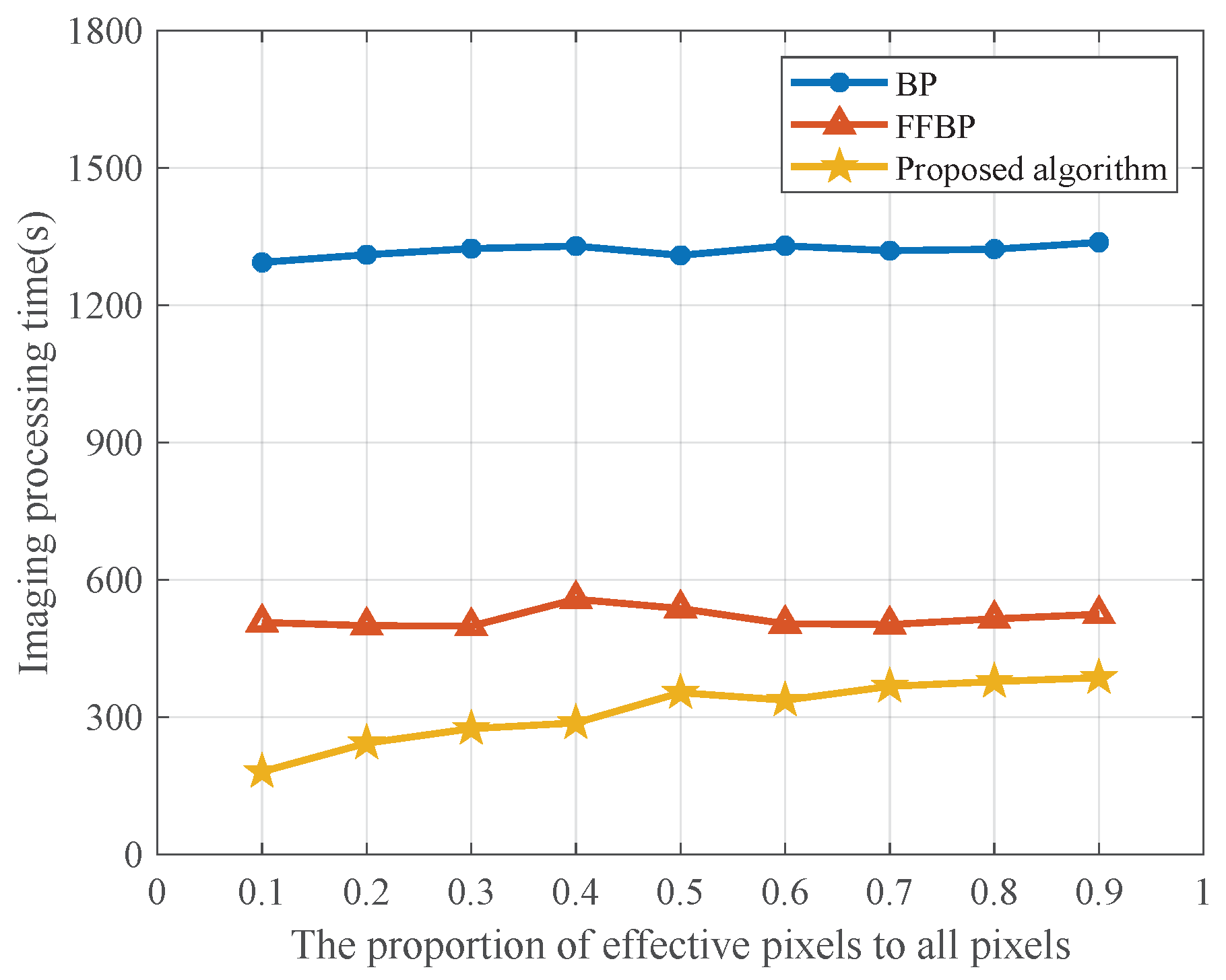
4.2. Computational Complexity Analysis

In the proposed algorithm, it is assumed that the MuA-SAR system contains N receivers, the full aperture length of each bistatic radar pair is $L_{An}$, the dimension of the original echo data are $L_{az}\times L_{rg}$, and the size of the imaging result obtained after recursive fusion is also $L_{az}\times L_{rg}$. The echo data are divided into $K_{sub}$ sub-apertures to complete imaging processing, respectively, and the size of the sub-image obtained after sub-aperture imaging processing is $\left(L_{An}/K_{sub}\right)\times L_{rg}$. The total number of fusion levels involved in the coherent fusion process is $G={log}_2{K}_{sub}$. The computational load in the proposed algorithm is mainly generated by the following three aspects:

(a) 

BP imaging process at the initial level.

In the process of BP imaging, the size of the echo data received by the full aperture is $L_{az}\times L_{rg}$, and the length of each sub-aperture is $L_{An}/K_{sub}$. At a range direction, it is necessary to complete the back projection of $L_{An}/K_{sub}$ echo data to the GCCS. The number of operations required in this process is $L_{az}·L_{rg}·L_{An}/K_{sub}$.

(b) 

The upsampling operation in coherent fusion process from level 0th to the level $\left(G-1\right)$.

In coherent fusion process from level g to level $\left(g+1\right)$, $2^{G-g}$ sub-images need to complete a two-times upsampling operation, and the number of pixels to be upsampled in each sub-image is $L_{rg}\times \left[L_{az}/\left(2^{G-g}\right)\right]$. Therefore, the maximum number of operations that need to be upsampled in the coherent fusion process between these two fusion levels is

$$2^{G-g}\times L_{rg}\times \left[L_{az}/\left(2^{G-g}\right)\right]=L_{rg}·L_{az}$$

(54)

Because the image segmentation method based on MSER is introduced into this imaging algorithm to segment the suspected target regions in the sub-images, not all pixels need to be upsampled. Assuming that at the $g\mathrm{th}$ level, the ratio of the number of pixels contained in the segmented extremal regions to the number of all pixels in the image is $m_i\left(i=1,2,\dots ,G-g\right)$, and set $m=max\left\{m_1,m_2,\dots ,m_{G-g}\right\}$, that is, the pixels with m in all pixels are segmented and upsampled at most. Therefore, the maximum number of operations required for upsampling in the process of sub-images coherent fusion from level 0 to level $\left(G-1\right)$ is

$$\sum _{g=0}^{G-1}m\times L_{rg}\times L_{az}\times \left(G-\mathrm{g}\right)=\frac{\left(G+1\right)G}{2}·m·L_{rg}·L_{az}$$

(55)

(c) 

The image segmentation process based on MSER from level 0 to level$\left(G-1\right)$.

At the $g\mathrm{th}$ level, $G-g$ sub-images need to be selected to segment the suspected target regions by MSER method, and the number of pixels in each sub-image in this fusion level is $L_{rg}\times L_{az}/2^{G-g}$. At each fusion level, firstly, the bin sort algorithm is needed to sort the gray values of all pixels in each sub-image selected for image segmentation at this fusion level, and the maximum number of operations required is

$$m\times \left(L_{rg}\times L_{az}/2^{G-g}\right)\times \left(G-g\right)=\frac{m·L_{rg}·L_{az}·\left(G-g\right)}{2^{G-g}}$$

(56)

Then, it also needs to use the union-find algorithm to store the list and area of the connection area. At each fusion level, the process requires a maximum number of operations.

$$\begin{array}{c}m\times L_{rg}\times L_{az}/2^{G-g}\times {log}_2\left[{log}_2\left(m\times L_{rg}\times L_{az}/2^{G-g}\right)\right]\times \left(G-g\right)\hfill \\ =\frac{m·L_{rg}·L_{az}·\left(G-g\right)}{2^{G-g}}·{log}_2\left[{log}_2\left(\frac{m·L_{rg}·L_{az}}{2^{G-g}}\right)\right]\hfill \end{array}$$

(57)

Therefore, the maximum number of operations required for the MSER-based image segmentation process from level 0 to level $\left(G-1\right)$ is

$$\sum _{g=0}^{G-1}\frac{m·L_{rg}·L_{az}·\left(G-g\right)}{2^{G-g}}+\frac{m·L_{rg}·L_{az}·\left(G-g\right)}{2^{G-g}}·{log}_2\left[{log}_2\left(\frac{m·L_{rg}·L_{az}}{2^{G-g}}\right)\right]$$

(58)

To summarize, the total number of operations required by this algorithm to complete an imaging process is

$$\begin{array}{c}{L}_{az}·L_{rg}·L_{An}/K_{sub}+\frac{\left(G-1\right)G}{2}·m·L_{rg}·L_{az}\hfill \\ +{\displaystyle \sum _{g=0}^{G-1}}\frac{m·L_{rg}·L_{az}·\left(G-g\right)}{2^{G-g}}+\frac{m·L_{rg}·L_{az}·\left(G-g\right)}{2^{G-g}}·{log}_2\left[{log}_2\left(\frac{m·L_{rg}·L_{az}}{2^{G-g}}\right)\right]\hfill \end{array}$$

(59)

Assuming that $L_{An}=L_{az}=L_{rg}=L$, and g and G in (59) are constants, the algorithm complexity of the proposed imaging algorithm is

$$O\left(L^3/K_{sub}\right)+O\left(m·L^2·{log}_2{K}_{sub}\right)+O\left(m·L^2\right)$$

(60)

Especially when the number of sub-apertures reaches $K_{sub}=L_{An}=L$, the computational complexity of this algorithm is mainly affected by the valid pixel ratio $m\left(0<m<1\right)$. It can be seen from (60) that the computational complexity of the proposed algorithm is between $O\left(L^2\right)$ and $O\left(L^2·{log}_{2}L\right)$, which is lower than that of the FFBP algorithm.

5. Simulation Experiments

In this section, to verify the performance and efficiency of the proposed imaging algorithm, the point target scene, and the two-dimensional (2D) surface target scene are processed by the BP algorithm, FFBP algorithm, and the proposed algorithm, respectively, and the imaging results and processing time are compared. Then, the 2D surface target scene with different effective target pixel ratios is set to compare and verify the efficiency improvement in the algorithm proposed for different scenes.

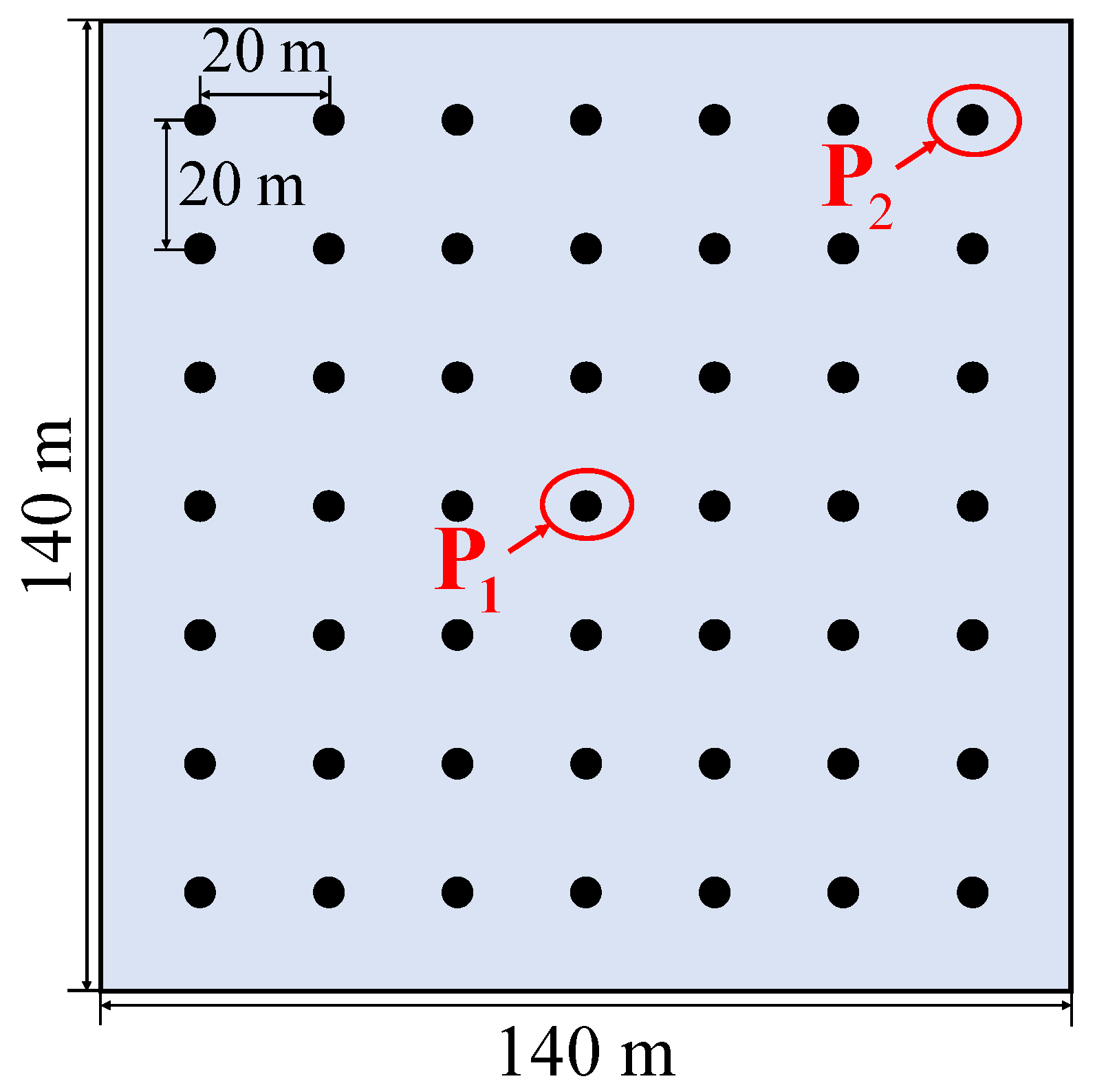
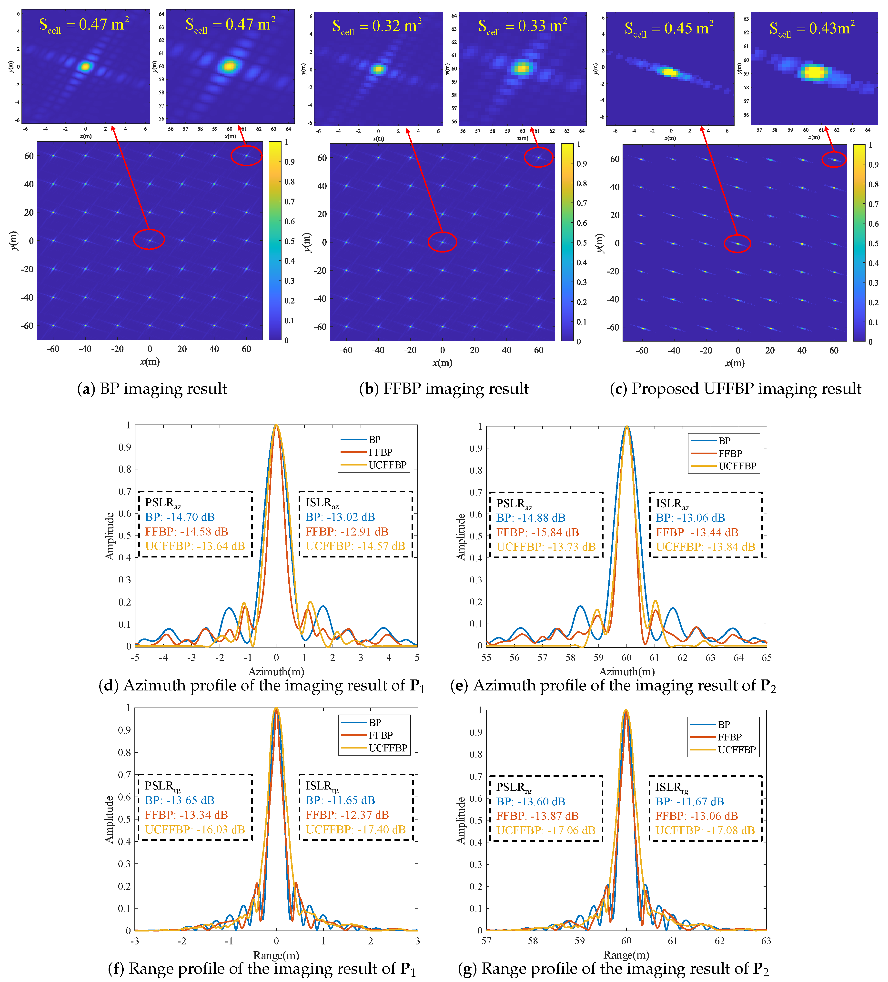
5.1. Point Target Simulation

The arrangement of point targets is shown in Figure 8. 49 point targets are evenly distributed in 7 rows and 7 columns in a scene with a size of $140\mathrm{m}\times 140\mathrm{m}$, and the distance between two adjacent point targets in the horizontal and vertical directions is $20\mathrm{m}$. Set the MuA-SAR system with one transmitter and two receivers to simulate the echo data. Use the BP algorithm, FFBP algorithm, and the proposed algorithm in this section for simulation, respectively, where the full aperture is divided into 64 sub-apertures, and the number of sub-images fusion levels is 6 in FFBP and the proposed algorithm. The simulation parameters are shown in

Table 2. Radar signal and geometric configuration parameters of simulation experiment.

Radar Signal Parameters		Geometric Configuration Parameters
Parameters	Value	Parameters	Value
Carrier frequency	9.6 GHz	Initial position of T	(7.32, 13.32, 5.00) km
Bandwidth	200 MHz	Velocity vector of T	(24.85, −147.93, 0.00) m/s
Sampling rate	220 MHz	Initial position of R1	(2.50, 15.00, 5.00) km
Pulse repetition frequency	1024 Hz	Velocity vector of R1	(0.00, −150.00, 0.00) m/s
Pulse time width	4 μs	Initial position of R2	(2.67, 14.99, 4.73) km
Synthetic aperture time	4 s	Velocity vector of R2	(−4.03, −149.95, 0.00) m/s

. The hardware platform of the simulation experiment is a workstation with Intel(R) Xeon(R) Gold 6130 2.10 GHz CPU, NVIDIA TITAN RTX 24 G GPU, and 256 G memory, and the simulation software is MATLAB R2023A.

Figure 9a–c show the imaging results of the point target using the BP algorithm, FFBP algorithm, and proposed UCFFBP algorithm, respectively. By comparison, the imaging effects of the three algorithms are close, and the proposed algorithm eliminates more sidelobe information than the other two algorithms. As shown in Figure 8, two point targets, ${\mathbf{P}}_1$ and ${\mathbf{P}}_2$, located at the center and edge of the scene, are selected to show their profiles along the azimuth direction using different algorithms. The profile results are shown in Figure 9d–f. Further, the peak sidelobe ratio (PSLR), integrated sidelobe level ratio (ISLR) along the azimuth and range direction, and the resolution unit area (${\mathrm{S}}_{\mathrm{cell}}$) of the two point targets are measured and listed in Figure 9 and

Table 3. Comparison of imaging performance of different algorithms.

Algorithm	Measured Parameters	Point Target P1	Point Target P2
	Scell (m2)	0.47	0.47
BP algorithm	PSLRaz/PSLRrg (dB)	−14.70/−13.65	−14.88/−13.60
	ISLRaz/ISLRrg (dB)	−13.02/−11.65	−13.06/−11.67
	Scell (m2)	0.32	0.33
FFBP	PSLRaz/PSLRrg (dB)	−14.58/−13.34	−15.84/−13.87
	ISLRaz/ISLRrg (dB)	−12.91/−12.37	−13.44/−13.06
	Scell (m2)	0.45	0.43
Proposed algorithm	PSLRaz/PSLRrg (dB)	−13.64/−16.03	−13.73/−17.06
	ISLRaz/ISLRrg (dB)	−14.57/−17.40	−13.84/−17.08

[15,49].

Then, in the same size scene, 49 point targets are randomly generated and set. The BP algorithm, FFBP algorithm, and the proposed algorithm are used for imaging processing. The repeated experiments are carried out for six times and the imaging processing time is recorded. The six groups’ results and average values are compared in

Table 4. Comparison of processing times of different algorithms.

Group	BP Algorithm	FFBP Algorithm	Proposed Algorithm
1	51.5	38.3	23.4
2	50.8	37.9	22.9
3	52.9	38.2	22.3
4	54.5	37.8	22.6
5	52.1	38.7	22.4
6	53.2	37.6	23.0
Average Value	52.5	38.1	22.8

.

According to the comparison of imaging results and processing time in Figure 9, and Table 3 and Table 4, several conclusions can be drawn about point target imaging. First, for the point ${\mathbf{P}}_1$, compared with BP algorithm, the ${\mathrm{S}}_{\mathrm{cell}}$ of the proposed algorithm is $0.02{\mathrm{m}}^2$ smaller than BP, and their focusing performance is similar. Compared with FFBP algorithm, the ${\mathrm{S}}_{\mathrm{cell}}$ of the proposed algorithm losses $0.13{\mathrm{m}}^2$. However, because there is no phase error in BP-based method, the phase error of the proposed algorithm is also small. Second, the $\mathrm{PSL}{\mathrm{R}}_{\mathrm{az}},\mathrm{ISL}{\mathrm{R}}_{\mathrm{az}},\mathrm{PSL}{\mathrm{R}}_{\mathrm{rg}}$, and $\mathrm{ISL}{\mathrm{R}}_{\mathrm{rg}}$ of the proposed algorithm are better than BP algorithm $1.06\mathrm{dB},1.55\mathrm{dB},2.38\mathrm{dB}$, and $5.75\mathrm{dB}$, respectively. Compared with FFBP algorithm, the $\mathrm{PSL}{\mathrm{R}}_{\mathrm{az}}$ of the proposed algorithm loses $0.94\mathrm{dB}$. The $\mathrm{ISL}{\mathrm{R}}_{\mathrm{az}},\mathrm{PSL}{\mathrm{R}}_{\mathrm{rg}}$, and $\mathrm{ISL}{\mathrm{R}}_{\mathrm{rg}}$ improve $1.66\mathrm{dB},2.69\mathrm{dB}$, and $5.03\mathrm{dB}$, respectively. The proposed algorithm has a good focusing effect on both the center and the edge of the scene, and has shorter sidelobe tail than BP algorithm and FFBP algorithm in azimuth, which is the advantage brought by introducing multi-level regional attention strategy based on the MSER image segmentation in the recursive fusion process. Finally, when the focusing performance is close to BP algorithm, the processing efficiency of the proposed algorithm is improved by about 56.6%, and when the phase error is smaller than FFBP algorithm, the processing efficiency of the proposed algorithm is still improved by about 40.2%.

5.2. 2D Surface Target Simulation

To verify the imaging performance and efficiency of the proposed algorithm for a 2D surface target, a $1.2\mathrm{km}\times 1.2\mathrm{km}$ SAR image of a bay scene is selected as the original scene. First, the size of the original scene is $800\times 800$ pixels. Second, the MuA-SAR system is simulated to generate echoes, and the simulation conditions and parameters are the same as those of point target simulation in Section 5.1. Then, the BP algorithm, FFBP algorithm, and the proposed algorithm are used for imaging processing, respectively. The processing time of the three methods are: BP algorithm, 1322.26 s; FFBP algorithm, 443.84 s; and the proposed algorithm, 293.47 s. Compared with the BP and FFBP algorithm, the efficiency of the proposed algorithm is improved by about 77.8% and 33.9%. The imaging results of the three algorithms are illustrated in Figure 10a–c. Two areas in the imaging results of different algorithms, area A and area B, are selected for enlarged display. Compared with the imaging results, it can be found that the imaging performance of the proposed algorithm is similar to that of the BP algorithm and FFBP algorithm, and the proposed algorithm can retain more target contour information and suppress background noise.

To further verify the efficiency improvement in the proposed method for different 2D surface targets, different surface target scenes with valid pixel ratios ranging from 0.1 to 0.9 are set at intervals of 0.1, and the above three imaging algorithms are used for imaging processing. The processing time is recorded, and the results are shown in Figure 11. It can be seen from Figure 11 that the imaging efficiency of the proposed method is greatly improved compared with the BP algorithm and FFBP algorithm for 2D surface targets with different valid pixels and the efficiency improvement effect is gradually weakened with the increase in valid pixels.

6. Discussion

Firstly, there is a phase difference between multiple bistatic radar pairs in the MuA-SAR system. In the existing methods, only the local coordinate system is established for analysis and processing, and the phase difference will lead to a serious decline in focusing performance. In the proposed method, the GCCS is established, and the coherent processing of data by different bistatic radars is realized by rotating WS alignment and phase compensation, which improves processing efficiency.

Secondly, there are differences among sub-images at different fusion levels of each platform. In the proposed method, a multi-level regional attention strategy based on MSER segmentation is implemented in some sub-images at each recursive fusion level, and the suspected target regions are segmented and merged. Under the condition of ensuring that the target pixel is not lost, the number of pixels that need recursive fusion is reduced, and the processing efficiency is further improved.

Thirdly, the segmentation method based on MSER is adopted in the multi-level regional attention strategy, and its segmentation accuracy has certain limitations. To ensure that the pixels in the suspected target regions are not missed, the lowest segmentation threshold in MSER is usually lower, which will result in some redundant pixels being retained. However, MSER segmentation is a threshold-based method, and its efficiency is much higher than that based on edge detection and clustering. Therefore, compared with the improvement in imaging processing efficiency, it is acceptable to lose the accuracy of some segmentation areas.

Finally, the requirements of the application of coherent processing of multi-static SAR are complex and are influenced by many factors, mainly including platform motion errors, time and frequency synchronization, and target scattering characteristics. These problems are solved in the existing work [50,51,52]. This paper mainly solves the fast-imaging problem of MuA-SAR. In the subsequent research, to improve the usability of coherent processing of multi-static SAR, many studies should be performed in the future, including geometric configuration design, and so on.

7. Conclusions

In this paper, a UCFFBP algorithm with multi-level regional attention strategy is proposed for MuA-SAR fast imaging. On the one hand, the GCCS is established, and echo data from different bistatic radar pairs can be processed uniformly and coherently, which avoids redundant operation and error accumulation. On the other hand, a multi-level regional attention strategy based on MSER image segmentation is proposed, and only the pixels in the suspected target regions at each fusion level are paid more attention for coherent fusion, which further improves processing efficiency. Simulation experimental data verify that the efficiency of the proposed algorithm can be improved by more than 50% and 30% compared with the BP and FFBP algorithms. The UCFFBP algorithm can not only ensure the imaging quality, but also improve the efficiency of imaging processing.

References

1. Gao, F.; Yang, Y.; Wang, J.; Sun, J.; Yang, E.; Zhou, H. A deep convolutional generative adversarial networks (DCGANs)-based semi-supervised method for object recognition in synthetic aperture radar (SAR) images. Remote Sens. 2018, 10, 846. [Google Scholar] [CrossRef]
2. Zhou, F.; Tian, T.; Zhao, B.; Bai, X.; Fan, W. Deception against near-field synthetic aperture radar using networked jammers. IEEE Trans. Aerosp. Electron. Syst. 2019, 55, 3365–3377. [Google Scholar] [CrossRef]
3. Fei, G.; Aidong, L.; Kai, L.; Erfu, Y.; Hussain, A. A novel visual attention method for target detection from SAR images. Chin. J. Aeronaut. 2019, 32, 1946–1958. [Google Scholar]
4. Baraha, S.; Sahoo, A.K. Synthetic Aperture Radar Image and its Despeckling using Variational Methods: A Review of Recent Trends. Signal Process. 2023, 212, 109156. [Google Scholar] [CrossRef]
5. Cumming, I.G.; Wong, F.H. Digital processing of synthetic aperture radar data. Artech House 2005, 1, 108–110. [Google Scholar]
6. Long, T.; Zeng, T.; Hu, C.; Dong, X.; Chen, L.; Liu, Q.; Xie, Y.; Ding, Z.; Li, Y.; Wang, Y.; et al. High resolution radar real-time signal and information processing. China Commun. 2019, 16, 105–133. [Google Scholar]
7. Lu, J.; Zhang, L.; Huang, Y.; Cao, Y. High-resolution forward-looking multichannel SAR imagery with array deviation angle calibration. IEEE Trans. Geosci. Remote Sens. 2020, 58, 6914–6928. [Google Scholar] [CrossRef]
8. Wu, J.; Yang, J.; Huang, Y.; Yang, H.; Wang, H. Bistatic forward-looking SAR: Theory and challenges. In Proceedings of the 2009 IEEE Radar Conference, Pasadena, CA, USA, 4–8 May 2009; pp. 1–4. [Google Scholar]
9. Chen, R.; Li, W.; Li, K.; Zhang, Y.; Yang, J. A Super-Resolution Scheme for Multichannel Radar Forward-Looking Imaging Considering Failure Channels and Motion Error. IEEE Geosci. Remote Sens. Lett. 2023, 20, 1–5. [Google Scholar] [CrossRef]
10. Mao, D.; Zhang, Y.; Pei, J.; Huo, W.; Zhang, Y.; Huang, Y.; Yang, J. Forward-looking geometric configuration optimization design for spaceborne-airborne multistatic synthetic aperture radar. IEEE J. Sel. Top. Appl. Earth Obs. Remote Sens. 2021, 14, 8033–8047. [Google Scholar] [CrossRef]
11. Santi, F.; Antoniou, M.; Pastina, D. Point spread function analysis for GNSS-based multistatic SAR. IEEE Geosci. Remote Sens. Lett. 2014, 12, 304–308. [Google Scholar] [CrossRef]
12. Krieger, G.; Moreira, A. Spaceborne bi-and multistatic SAR: Potential and challenges. IEE Proc.-Radar Sonar Navig. 2006, 153, 184–198. [Google Scholar] [CrossRef]
13. Krieger, G.; Zonno, M.; Rodriguez-Cassola, M.; Lopez-Dekker, P.; Mittermayer, J.; Younis, M.; Huber, S.; Villano, M.; De Almeida, F.Q.; Prats-Iraola, P.; et al. MirrorSAR: A fractionated space radar for bistatic, multistatic and high-resolution wide-swath SAR imaging. In Proceedings of the 2017 IEEE International Geoscience and Remote Sensing Symposium (IGARSS), Fort Worth, TX, USA, 23–28 July 2017; pp. 149–152. [Google Scholar]
14. Moccia, A.; Renga, A. Spatial resolution of bistatic synthetic aperture radar: Impact of acquisition geometry on imaging performance. IEEE Trans. Geosci. Remote Sens. 2011, 49, 3487–3503. [Google Scholar] [CrossRef]
15. Xu, F.; Zhang, Y.; Wang, R.; Mi, C.; Zhang, Y.; Huang, Y.; Yang, J. Heuristic path planning method for multistatic UAV-borne SAR imaging system. IEEE J. Sel. Top. Appl. Earth Obs. Remote Sens. 2021, 14, 8522–8536. [Google Scholar] [CrossRef]
16. Smith, A. A new approach to range-Doppler SAR processing. Int. J. Remote Sens. 1991, 12, 235–251. [Google Scholar] [CrossRef]
17. Hughes, W.; Gault, K.; Princz, G. A comparison of the Range-Doppler and Chirp Scaling algorithms with reference to RADARSAT. In Proceedings of the IGARSS’96, 1996 International Geoscience and Remote Sensing Symposium, Lincoln, NE, USA, 31 May 1996; Volume 2, pp. 1221–1223. [Google Scholar]
18. Li, C.; Zhang, H.; Deng, Y.; Wang, R.; Liu, K.; Liu, D.; Jin, G.; Zhang, Y. Focusing the L-band spaceborne bistatic SAR mission data using a modified RD algorithm. IEEE Trans. Geosci. Remote Sens. 2019, 58, 294–306. [Google Scholar] [CrossRef]
19. Rigling, B.D.; Moses, R.L. Polar format algorithm for bistatic SAR. IEEE Trans. Aerosp. Electron. Syst. 2004, 40, 1147–1159. [Google Scholar] [CrossRef]
20. Sun, J.; Mao, S.; Wang, G.; Hong, W. Polar Format Algorithm for Spotlight Bistatic Sar with Arbitrary Geometry Configuration. Prog. Electromagn. Res. 2010, 103, 323–338. [Google Scholar] [CrossRef]
21. Cumming, I.G.; Neo, Y.L.; Wong, F.H. Interpretations of the omega-K algorithm and comparisons with other algorithms. In Proceedings of the IGARSS 2003 IEEE International Geoscience and Remote Sensing Symposium (IEEE Cat. No. 03CH37477), Toulouse, France, 21–25 July 2003; Volume 3, pp. 1455–1458. [Google Scholar]
22. Liu, B.; Wang, T.; Wu, Q.; Bao, Z. Bistatic SAR data focusing using an omega-K algorithm based on method of series reversion. IEEE Trans. Geosci. Remote Sens. 2009, 47, 2899–2912. [Google Scholar]
23. Zhu, R.; Zhou, J.; Tang, L.; Kan, Y.; Fu, Q. Frequency-domain imaging algorithm for single-input–multiple-output array. IEEE Geosci. Remote Sens. Lett. 2016, 13, 1747–1751. [Google Scholar] [CrossRef]
24. Gaibel, A.; Boag, A. Back-projection SAR imaging using FFT. In Proceedings of the 2016 European Radar Conference (EuRAD), London, UK, 5–7 October 2016; pp. 69–72. [Google Scholar]
25. Zeng, D.; Zeng, T.; Hu, C.; Long, T. Back-projection algorithm characteristic analysis in forward-looking bistatic SAR. In Proceedings of the 2006 CIE International Conference on Radar, Shanghai, China, 16–19 October 2006; pp. 1–4. [Google Scholar]
26. McCorkle. Focusing of synthetic aperture ultra wideband data. In Proceedings of the IEEE 1991 International Conference on Systems Engineering, Dayton, OH, USA, 1–3 August 1991; pp. 1–5. [Google Scholar]
27. Yang, Y.; Pi, Y.; Li, R. Back projection algorithm for spotlight bistatic SAR imaging. In Proceedings of the 2006 CIE International Conference on Radar, Shanghai, China, 16–19 October 2006; pp. 1–4. [Google Scholar]
28. Feng, D.; An, D.; Huang, X. An extended fast factorized back projection algorithm for missile-borne bistatic forward-looking SAR imaging. IEEE Trans. Aerosp. Electron. Syst. 2018, 54, 2724–2734. [Google Scholar] [CrossRef]
29. Xiao, S.; Munson, D.C.; Basu, S.; Bresler, Y. An N 2 logN back-projection algorithm for SAR image formation. In Proceedings of the Thirty-Fourth Asilomar Conference on Signals, Systems and Computers (Cat. No. 00CH37154), Pacific Grove, CA, USA, 29 October–1 November 2000; Volume 1, pp. 3–7. [Google Scholar]
30. McCorkle, J.W.; Rofheart, M. Order N^2 log (N) backprojector algorithm for focusing wide-angle wide-bandwidth arbitrary-motion synthetic aperture radar. In Proceedings of the Radar Sensor Technology, Orlando, FL, USA, 8–9 April 1996; Volume 2747, pp. 25–36. [Google Scholar]
31. Yegulalp, A.F. Fast backprojection algorithm for synthetic aperture radar. In Proceedings of the 1999 IEEE Radar Conference, Radar into the Next Millennium (Cat. No. 99CH36249), Waltham, MA, USA, 22 April 1999; pp. 60–65. [Google Scholar]
32. Ding, Y.; Munson, D.J. A fast back-projection algorithm for bistatic SAR imaging. In Proceedings of the International Conference on Image Processing, Rochester, NY, USA, 22–25 September 2002; Volume 2, p. 2. [Google Scholar]
33. Ulander, L.M.; Hellsten, H.; Stenstrom, G. Synthetic-aperture radar processing using fast factorized back-projection. IEEE Trans. Aerosp. Electron. Syst. 2003, 39, 760–776. [Google Scholar] [CrossRef]
34. Wang, C.; Zhang, Q.; Hu, J.; Shi, S.; Li, C.; Cheng, W.; Fang, G. An Efficient Algorithm Based on Frequency Scaling for THz Stepped-Frequency SAR Imaging. IEEE Trans. Geosci. Remote Sens. 2022, 60, 1–15. [Google Scholar] [CrossRef]
35. Ulander, L.M.; Froelind, P.O.; Gustavsson, A.; Murdin, D.; Stenstroem, G. Fast factorized back-projection for bistatic SAR processing. In Proceedings of the 8th European Conference on Synthetic Aperture Radar, VDE, Aachen, Germany, 7–10 June 2010; pp. 1–4. [Google Scholar]
36. Zhou, S.; Yang, L.; Zhao, L.; Wang, Y.; Zhou, H.; Chen, L.; Xing, M. A new fast factorized back projection algorithm for bistatic forward-looking SAR imaging based on orthogonal elliptical polar coordinate. IEEE J. Sel. Top. Appl. Earth Obs. Remote Sens. 2019, 12, 1508–1520. [Google Scholar] [CrossRef]
37. Zhang, L.; Li, H.L.; Qiao, Z.J.; Xu, Z.W. A fast BP algorithm with wavenumber spectrum fusion for high-resolution spotlight SAR imaging. IEEE Geosci. Remote Sens. Lett. 2014, 11, 1460–1464. [Google Scholar] [CrossRef]
38. Sun, H.; Sun, Z.; Chen, T.; Miao, Y.; Wu, J.; Yang, J. An Efficient Backprojection Algorithm Based on Wavenumber-Domain Spectral Splicing for Monostatic and Bistatic SAR Configurations. Remote Sens. 2022, 14, 1885. [Google Scholar] [CrossRef]
39. Guo, Y.; Suo, Z.; Jiang, P.; Li, H. A Fast Back-Projection SAR Imaging Algorithm Based on Wavenumber Spectrum Fusion for High Maneuvering Platforms. Remote Sens. 2021, 13, 1649. [Google Scholar] [CrossRef]
40. Dong, Q.; Yang, Z.; Sun, G.; Xing, M. Cartesian factorized backprojection algorithm for synthetic aperture radar. In Proceedings of the 2016 IEEE International Geoscience and Remote Sensing Symposium (IGARSS), Beijing, China, 10–15 July 2016; pp. 1074–1077. [Google Scholar]
41. Dong, Q.; Sun, G.C.; Yang, Z.; Guo, L.; Xing, M. Cartesian factorized backprojection algorithm for high-resolution spotlight SAR imaging. IEEE Sens. J. 2017, 18, 1160–1168. [Google Scholar] [CrossRef]
42. Li, Y.; Xu, G.; Zhou, S.; Xing, M.; Song, X. A novel CFFBP algorithm with noninterpolation image merging for bistatic forward-looking SAR focusing. IEEE Trans. Geosci. Remote Sens. 2022, 60, 1–16. [Google Scholar] [CrossRef]
43. Xu, F.; Wang, R.; Frey, O.; Huang, Y.; Mi, C.; Mao, D.; Yang, J. Spatial Configuration Design for Multistatic Airborne SAR Based on Multiple Objective Particle Swarm Optimization . IEEE Trans. Geosci. Remote Sens. 2023, 61, 1–16. [Google Scholar]
44. Zeng, T.; Cherniakov, M.; Long, T. Generalized approach to resolution analysis in BSAR. IEEE Trans. Aerosp. Electron. Syst. 2005, 41, 461–474. [Google Scholar] [CrossRef]
45. Dower, W.; Yeary, M. Bistatic SAR: Forecasting spatial resolution. IEEE Trans. Aerosp. Electron. Syst. 2018, 55, 1584–1595. [Google Scholar] [CrossRef]
46. Matas, J.; Chum, O.; Urban, M.; Pajdla, T. Robust wide-baseline stereo from maximally stable extremal regions. Image Vis. Comput. 2004, 22, 761–767. [Google Scholar] [CrossRef]
47. Donoser, M.; Bischof, H. Efficient maximally stable extremal region (MSER) tracking. In Proceedings of the 2006 IEEE Computer Society Conference on Computer Vision and Pattern Recognition (CVPR’06), New York, NY, USA, 17–22 June 2006; Volume 1, pp. 553–560. [Google Scholar]
48. Wang, R.; Xu, F.; Pei, J.; Wang, C.; Huang, Y.; Yang, J.; Wu, J. An improved faster R-CNN based on MSER decision criterion for SAR image ship detection in harbor. In Proceedings of the IGARSS 2019 IEEE International Geoscience and Remote Sensing Symposium, Yokohama, Japan, 28 July–2 August 2019; pp. 1322–1325. [Google Scholar]
49. Pu, W.; Wu, J.; Huang, Y.; Li, W.; Sun, Z.; Yang, J.; Yang, H. Motion errors and compensation for bistatic forward-looking SAR with cubic-order processing. IEEE Trans. Geosci. Remote Sens. 2016, 54, 6940–6957. [Google Scholar] [CrossRef]
50. Wang, W.Q. GPS-based time & phase synchronization processing for distributed SAR. IEEE Trans. Aerosp. Electron. Syst. 2009, 45, 1040–1051. [Google Scholar]
51. Krieger, G.; Younis, M. Impact of oscillator noise in bistatic and multistatic SAR. IEEE Geosci. Remote Sens. Lett. 2006, 3, 424–428. [Google Scholar] [CrossRef]
52. Potter, L.C.; Moses, R.L. Attributed scattering centers for SAR ATR. IEEE Trans. Image Process. 1997, 6, 79–91. [Google Scholar] [CrossRef]
Figure 1. Spatial geometric configuration of MuA-SAR system.
Remotesensing 15 05183 g001
Figure 2. Distribution principle of WS.
Remotesensing 15 05183 g002
Figure 3. WS in different states. (a) The k a directions of WS of different receivers are inconsistent, (b) the k a directions of WS of different receivers are consistent.
Remotesensing 15 05183 g003
Figure 4. Shifting and folding of sub-aperture WS and the analysis of aliasing phenomenon of the WS. (a) Shifting and folding of sub-aperture WS of center point target, (b) the WS distribution when the grid division resolution is equal to the theoretical value, (c) the WS distribution when the grid division resolution is much higher than the theoretical value, (d) BP imaging results of randomly distributed point targets corresponding to the WS in (b), (e) BP imaging results of randomly distributed point targets corresponding to the WS in (c).
Remotesensing 15 05183 g004
Figure 5. Flowchart of the proposed imaging algorithm.
Remotesensing 15 05183 g005
Figure 6. Schematic diagram of rotated coordinate system. (a) The rotated new Cartesian coordinate system u O v , (b) the transmitter’s local coordinate system u O v and the receiver’s local coordinate system u O v .
Remotesensing 15 05183 g006
Figure 7. Schematic diagram of image segmentation method based on MSER.
Remotesensing 15 05183 g007
Figure 8. Target distribution map of point target scene.
Remotesensing 15 05183 g008
Figure 9. Comparison of point target imaging performance. (a) BP algorithm result, (b) FFBP algorithm result, (c) imaging result of the proposed UCFFBP algorithm, (d) profile of the imaging result of P 1 along the azimuth direction, (e) profile of the imaging result of P 2 along the azimuth direction, (f) profile of the imaging result of P 1 along the range direction, (g) profile of the imaging result of P 2 along the range direction.
Remotesensing 15 05183 g009
Figure 10. Comparison of 2D surface target imaging performance. (a) BP algorithm result, (b) FFBP algorithm result, (c) imaging result of the proposed UCFFBP algorithm.
Remotesensing 15 05183 g010
Figure 11. Comparison of processing time of 2D surface targets with different valid pixel ratios.
Remotesensing 15 05183 g011