Reconstruction of Land Surface Temperature Derived from FY-4A AGRI Data Based on Two-Point Machine Learning Method

Abstract

Land surface temperature (LST) is one of the most important parameters of the interface between the earth surface and the atmosphere, and it plays a significant role in many research fields, such as agriculture, climate, hydrology, and the environment. However, the thermal infrared band of remote sensors is easily affected by clouds and aerosols, leading to many data gaps in LST products, which restricts the subsequent application of these products. In this paper, Beijing, China, is selected as the study area, and the LST data retrieved from Fengyun 4A (FY-4A) Advanced Geosynchronous Radiation Imager (AGRI) are reconstructed based on the two-point machine learning method. Firstly, the two-point machine learning model is built to reconstruct the theoretical clear-sky LST from simulated and actual images, and the accuracy of the reconstruction results is evaluated compared with the random forest algorithm and the inverse distance weighted method. Secondly, the actual LST under the influence of clouds is reconstructed by using the ERA5 reanalysis LST data as the auxiliary data, and the reconstruction accuracy is then evaluated by the field measurement LST data. The experimental results show that (1) the prediction accuracy of the two-point machine learning method is higher than that of the random forest method in both simulated data and actual data experiments; (2) the R² of reconstructed LST under theoretical clear-sky conditions is 0.6860 and the root mean square error (RMSE) is 2.9 K, while the R² of the reconstructed accuracy of actual LST under clouds is 0.7275 and the RMSE is 2.6 K, i.e., the RMSE decreases by 10.34%; (3) the two-point machine method combined with the auxiliary ERA5 LST data can well reconstruct LST under cloudy conditions and present a reasonable LST distribution.

1. Introduction

Land surface temperature (LST) is a key parameter in environmental monitoring and ecological processes [1,2], which is of great importance in many research fields, such as meteorology, hydrology, and climatology [3]. The main traditional method of obtaining LST is ground-based measurements, which have the advantage of relatively high accuracy, but it is difficult to obtain a uniform and continuous distribution of LST data due to the limited geographical conditions. With the rapid development of remotely sensed technology, both thermal infrared sensors under clear-sky conditions and microwave sensors can provide spatially continuous LST data, and thermal infrared sensors can retrieve the LST data with higher spatial resolution. However, thermal infrared sensors often suffer from various degrees of temporal and spatial deficiencies due to the influence of cloud cover and aerosols [4], limiting the further application of existing LST data. To meet the demand of LST data application in a variety of research fields, missing gaps in LST data must be filled and reconstructed.

How to reconstruct the LST pixels under clouds to generate seamless all-weather LST data has become a research hotspot in thermal infrared remote sensing. In recent years, many studies have tried to fill the LST data gaps under cloudy conditions. The existing reconstruction methods can be divided into three categories: spatial gap-filling methods [5,6], temporal gap-filling methods [7,8], and combined spatiotemporal gap-filling methods [9,10]. The spatial gap-filling methods consider the continuous character of LST spatial distribution and use spatially adjacent clear-sky LST data to reconstruct the missing LST data under cloudy skies. This type of method is easy to be implemented and has good reconstruction results for a small range of missing data, but the accuracy decreases significantly as the number of missing pixels increases. Moreover, spatial gap-filling methods are mainly suitable for the data with higher spatial resolution. When the spatial resolution decreases, the LST spatial correlation worsens, and the accuracy of the reconstruction will also decrease. Temporal gap-filling methods fill the LST data under cloudy conditions using clear-sky LST data at an adjacent time for the same area, and these algorithms mainly include linear interpolation, harmonic analysis, time Fourier analysis, diurnal temperature cycle (DTC) methods, etc. DTC methods are usually used to reconstruct LST data from geostationary meteorological satellites, and this type of method is affected by the model parameters. The fitting precision improves as the number of model parameters increases, but usually leads to a decrease in the efficiency [9], and satisfactory reconstruction results cannot be achieved when the number of clear-sky pixels is less than the model parameters. The spatiotemporal gap-filling methods integrate the spatiotemporal information of LST data, which solve the existing deficiencies in temporal and spatial interpolation to a certain extent, but their reconstruction accuracy depends on the quality and quantity of the clear-sky LST pixels.

Among these three types of gap-filling methods, spatial gap-filling methods are more commonly used. Traditional spatial interpolation methods, including inverse distance weight interpolation [11,12], spline function interpolation [13,14], and kriging interpolation [4,11,12], have been widely used by researchers. Tu et al. [4] estimated missing LST values under cloudy skies based on ordinary kriging interpolation and regular spline function interpolation methods, and the results showed that these two methods are suitable in the case of missing LST under discrete and small cloudy patches, but these two methods are not applicable to estimate LST under continuous clouds, and the accuracy of the reconstruction result decreases significantly when there is a large amount of clouds. A comprehensive analysis of existing studies shows that the traditional spatial interpolation methods have a large error in estimating LST because the vegetation distribution, topographic relief, and geographic location have an effect on LST distribution. To improve the accuracy of LST reconstruction, a simple linear regression model between LST and the influencing environmental parameters has been developed [15]. Ke et al. [15] applied a combined regression kriging algorithm using longitude, latitude, digital elevation model (DEM), normalized difference vegetation index (NDVI), and other factors as input variables to reconstruct 8-day synthetic MODIS LST data from 2003 to 2010 for the central region of the Tibetan Plateau. The results showed that the addition of auxiliary variables, such as DEM and NDVI, can improve the accuracy of LST reconstruction in complex terrain regions, but the accuracy was relatively lower under the conditions of dense or extensive clouds.

Previous studies on reconstructing LST mainly focused on polar orbiting sensors like MODIS [6,8,13,15], while fewer studies have used LST data retrieved from geostationary satellites. Geostationary meteorological satellites, such as Fengyun 2 and Fengyun 4, have a higher temporal resolution of up to the minute level. Many researchers have made progress in utilizing LST data from these satellites for missing data reconstruction and various applications. Wu et al. [14] used a multi-scale feature-connected convolutional neural network (CNN) model to reconstruct the missing values from FY-2G Visible and Infrared Spin Scan Radiometer-II (VISSR-II) and MSG Spinning Enhanced Visible and Infrared Imager (SEVIRI) LST, and the root mean square errors (RMSEs) were mostly smaller than 0.8 K. Lu et al. [5] developed a time-neighborhood pixel method for cloud-covered pixels in MSG SEVIRI LST, and the results showed that the mean absolute error (MAE) of the reconstructed LST was less than 1.5 K in the best case. Liu et al. [11] introduced genetic algorithms (GAs) as a temporal gap-filling method, and the spectral multi-metamorphic clustering (SMMC) algorithm combined with inverse distance weighting (IDW) as a spatial reconstruction approach, to reconstruct FY-2F LST pixels under cloudy conditions with an accuracy within 2 K. Zhao et al. [16] utilized accumulated solar radiation, leaf area index, and elevation as predictors to build a random forest (RF) algorithm for estimating LST under cloudy conditions, which was compared with Global Land Data Assimilation System (GLDAS) LST. Wu [17] used an RF-based algorithm to reconstruct LST and then downscaled the spatial resolution from 5 km to 1 km, and the results indicated that the RF algorithm outperformed traditional statistical regression methods in terms of reconstruction accuracy.

The LST reconstruction methods mentioned above typically provide estimates of theoretical clear-sky LST rather than actual LST under clouds. These methods exhibit high reconstruction accuracy when there are few missing LST values, but the accuracy decreases when there is a large area of missing data. The LST differences at different locations are highly correlated with the variations in land surface parameters at those locations; this correlation may be more significant than the relationship between LST and surface parameters at a specific location. Therefore, in this study, in order to improve the completeness and accuracy of the FY-4A AGRI LST, the two-point machine learning (TPML) method [18] from the spatial perspective is applied to reconstruct missing LST data, which are compared with the IDW method and the RF model. Moreover, this study further corrects the theoretical clear-sky LST to the actual LST under cloudy conditions using the ERA5 LST data as auxiliary information, which is of great significance for the quantitative application of FY-4A LST data in meteorological forecasting, natural disaster monitoring, and climate change research.

2. Study Area and Data

2.1. Study Area

Beijing, China, was chosen as the study area for both simulated data experiments and actual data experiments. The geographical range of Beijing is between 39.5° N and 40.1° N, and 115.4° E and 117.5° E. Beijing has 16 districts with a total area of 16,410.54 km². The city is mainly mountainous, accounting for 62% of the total area, while the rest is plain. The climate of Beijing is classified as warm temperate semiarid monsoon climate, characterized by high temperature and rainfall during the summer season.

2.2. Data

2.2.1. FY-4A AGRI LST Data

FY-4A is China’s second-generation geostationary quantitative remotely sensed satellite and one of the world’s most advanced geostationary meteorological satellites [19]. It was successfully launched on 11 December 2016 [20] and is equipped with various observation instruments, including the advanced geosynchronous radiation imager (AGRI), the geostationary interferometric infrared sounder (GIIRS), the lightning mapping imager (LMI), and the space environment monitoring instrument package (SEP) [21]. The FY-4A satellite provides a variety of products, including LST data. In this study, the experimental data of FY-4A AGRI LST was downloaded from the official website of the National Meteorological Satellite Center (http://www.nsmc.org.cn/, accessed on 1 January 2020).

The FY-4A AGRI LST data are stored in the NC format, with a spatial resolution of 4 km. The data are geometrically corrected using the latitude and longitude lookup table provided on the website. The geometrically corrected dataset is then cropped based on the administrative boundary vector data of the study area. For the simulated data experiments, LST data with a completely clear-sky condition on 1 October 2021 are selected. For the actual data experiments, 18 instances with missing data rates ranging from 30% to 95% are randomly selected. The missing rate and imaging time of the AGRI LST data used are shown in

Table 1. The imaging time and missing rate of the FY-4A AGRI LST data used in the study.

Data	Imaging Time (Beijing Time)	Missing Rate/%
Data used for simulated experiments	2021-10-01 17:00	0
	2021-10-01 10:00	61.10
	2021-10-01 22:00	65.41
	2021-10-01 08:00	88.81
	2021-10-01 09:00	86.51
	2021-10-01 10:00	60.55
	2021-10-02 01:00	84.77
	2021-10-07 06:00	58.44
	2021-10-07 08:00	75.87
	2021-10-08 10:00	38.17
Data of real experiments	2021-10-08 13:00	74.95
	2021-10-10 01:00	63.67
	2021-10-10 02:00	75.23
	2021-10-10 03:00	75.50
	2021-10-10 04:00	81.10
	2021-10-10 05:00	91.93
	2021-10-10 07:00	81.74
	2021-10-10 09:00	88.81
	2021-10-10 19:00	67.06

.

2.2.2. MOD09A1 Data

To avoid the influence of cloud cover on the acquisition of surface remotely sensed parameters during AGRI imaging time, 8-day synthetic MODIS data are selected to build the reconstruction model. The MOD09A1 dataset was chosen, which includes 8-day synthetic reflectance data stored in HDF format. It has a spatial resolution of 500 m and contains surface reflectance data of MODIS bands 1–7. The MOD09A1 data have been corrected for atmospheric conditions, such as gases, aerosols, and Rayleigh scattering. In addition to seven reflectivity bands, the data also include a mass layer and four observational angle bands. To process the MOD09A1 data, the MODIS Reprojection Tool (MRT) was utilized for reading, projection conversion, and mosaic processing. NDVI, Normalized Difference Building Index (NDBI), Modified Normalized Difference Water Index (MNDWI), Soil Adjusted Vegetation Index (SAVI), and Normalized Multiband Drought Index (NMDI) were calculated using MOD09A1 data. The MOD09A1 data were downloaded from the official website of Google Earth Engine (GEE) (https://earthengine.google.com/, accessed on 20 December 2019), and the data acquisition date was 30 September 2021.

2.2.3. Sentinel-3A LST Data

The Sentinel-3A satellite, launched by the European Space Agency (ESA) in 2016, carried the Sea and Land Surface Temperature Radiometer (SLSTR). SLSTR has two thermal infrared channels and can provide global sea and land surface temperature measurements with a spatial resolution of 1 km. For this study, Sentinel-3A SLSTR Level 2 LST data acquired at 10:21 h Beijing Time on 1 October 2021 were selected. To match with the spatial resolution of the FY-4A AGRI LST data, the 1-km resolution SLSTR LST data were resampled to 4 km, and were used as the reference to evaluate the theoretical clear-sky reconstruction results.

2.2.4. ERA5 Reanalysis LST Data

ERA5 is the fifth generation of the atmospheric reanalysis dataset produced by the European Centre for Medium-Range Weather Forecasts (ECMWF). It provides hour-by-hour reanalysis information since 1979. For this study, the ERA5-Land dataset was selected as the auxiliary data to estimate the actual cloudy-sky AGRI LST. It has a spatial resolution of 0.1 °C and a temporal resolution of 1 h. The data were obtained from the ECMWF website (https://cds.climate.copernicus.eu/, accessed on 17 December 2019).

2.2.5. DEM Data

The Shuttle Radar Topography Mission (SRTM) DEM data, jointly measured by the National Aeronautics and Space Administration (NASA) and the National Imagery and Mapping Agency (NIMA) of the Department of Defense, with a spatial resolution of 90 m, were downloaded from https://srtm.csi.cgiar.org, accessed on 15 December 2019. The DEM data underwent preprocessing steps, including stitching, projection conversion, and cropping. From the DEM data, the slope and aspect were calculated and upscaled to 4 km resolution to serve as auxiliary variables for the reconstruction model.

2.2.6. Field-Measured LST Data

Hourly LST observation data from 20 meteorological stations in Beijing in October 2021 were selected. The ground temperature was measured over a 200 cm (north-south) × 400 cm (east-west) loose and flat bare ground area in the observation field of the meteorological stations. The stations are generally selected to respond to the natural conditions of the local land surface, with a better representation. The measured data from the ground meteorological stations in this study have undergone quality control to ensure their reliability.

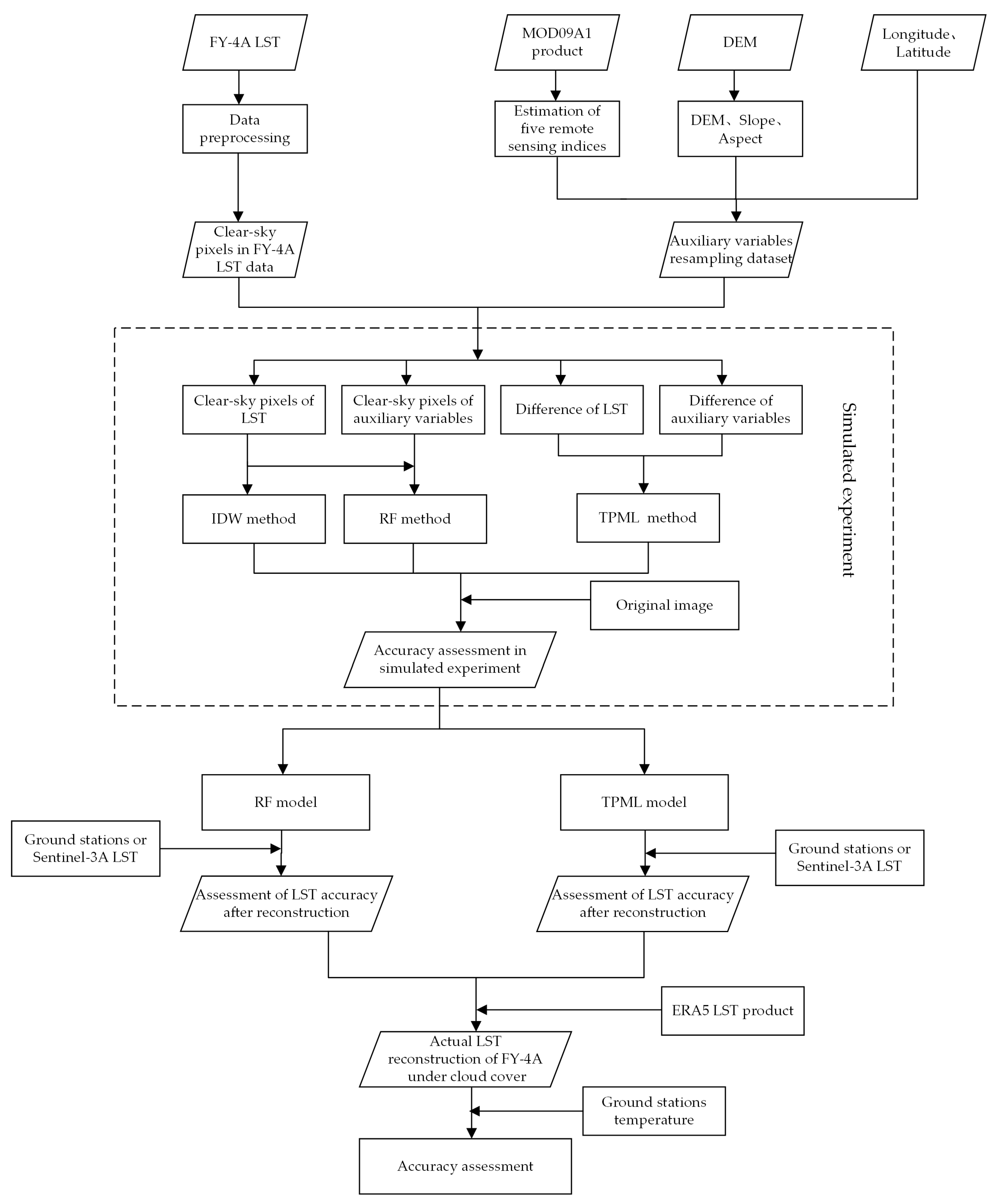
3. Research Methodology

The aim of this study is to enhance the completeness and accuracy of FY-4A LST data by reconstructing the actual LST under cloud cover. The research technology flowchart is shown in Figure 1. The first step is data preprocessing, including geometric correction and regional cropping. Five remotely sensed indices (NDVI, NDBI, MNDWI, NDMI, SAVI) are calculated using MOD09A1 reflectance data. The slope and the slope aspect data are obtained from the DEM data. Eight datasets are then resampled to 4-km resolution using the aggregated average method. In the second step, the RF model and the TPML model are constructed through simulated experiments. These models were built using the clear-sky AGRI LST and auxiliary variable images, which are then compared with the IDW method. Thirdly, the accuracy of the reconstruction results derived from the RF and TPML model is evaluated by using the station-measured LST and the Sentinel-3A LST data. In the fourth step, the relationship between the clear-sky AGRI LST and the ERA5 LST at the corresponding locations is used to reconstruct the actual LST under cloud cover, which is lastly evaluated using the field-measured LST.

3.1. Calculation of Remotely Sensed Spectral Indices

The spatial and temporal variations of LST are very complex and highly influenced by many biophysical variables, such as vegetation cover, soil moisture status, and topographic parameters like elevation and slope. By comprehensively analyzing the relevant research results on the mechanism of LST change [22,23], we choose five remotely sensed indices (NDVI, NDBI, MNDWI, NDMI, SAVI) as the auxiliary variables for the LST reconstruction model. NDVI reflects the vegetation growth status, vegetation cover, and other important vegetation physical properties. NDBI accurately reflects the information on buildings, with higher values indicating a higher proportion and density of buildings. MNDWI reflects the information on water bodies and can be used to distinguish between shadows and water bodies. NDMI effectively captures the moisture content of the vegetation canopies. SAVI indicates different reflectance for various soil types.

The five remotely sensed indices were calculated using the preprocessed MOD09A1 data; the calculation formulas [24] are shown in

Table 2. Remotely sensed spectral indices required for LST reconstruction.

Variables	Index Features	Calculation Formulas
MNDWI	Reflects water information	$MNDWI=\frac{\rho 4-\rho 6}{\rho 4+\rho 6}$
NDBI	Reflects building information	$NDBI=\frac{\rho 7-\rho 2}{\rho 7+\rho 2}$
NDMI	Reflects vegetation water content	$NDMI=\frac{\rho 2-\rho 6}{\rho 2+\rho 6}$
NDVI	Characterizes vegetation cover and growth status	$NDVI=\frac{\rho 2-\rho 1}{\rho 2+\rho 1}$
SAVI	Elimination of soil background disturbances	$SAVI=\frac{\rho 2-\rho 1}{\rho 2+\rho 1+L}\left(1+L\right)$ L = 0.5

. In Table 2, ${\rho }_1$, ${\rho }_2$, ${\rho }_4$, ${\rho }_6$, and ${\rho }_7$ represent the surface reflectance of MODIS bands 1, 2, 4, 6, and 7. The names and wavelengths of these bands are red (620–670 nm), near-infrared (841–876 nm), green (545–565 nm), short-wave infrared (1628–1652 nm), and short-wave infrared (2105–2155 nm), respectively. The central wavelengths for these bands are 645 nm, 859 nm, 555 nm, 1640 nm, and 2130 nm, respectively.

3.2. Simulated LST Data with Different Cloud Fraction Covers

Due to the spatial scale difference between the field-measured data and FY-4A AGRI LST data, and the time–space–angle difference between the data from different satellites, it is challenging to obtain actual LST data that can perfectly match with the FY-4A AGRI observations. Therefore, accurately evaluating the reconstructed LST under cloud cover is difficult. To solve this problem, a simulated method is employed. Some clear-sky pixels are artificially set as missing pixels, and their original LST values are used to compare with the reconstructed results, so that the accuracy of the different methods can be better compared and analyzed [9,14,25,26].

Since the FY-4A AGRI LST data are usually missing in blocky areas under cloudy conditions, in order to compare the reconstruction results of three different methods for various LST missing conditions, the FY-4A AGRI LST data imaged at 17:00 h Beijing time on 1 October 2021 under completely clear sky was selected. Areas with three different missing proportions (90.83%, 83.58%, and 70%) were artificially set to be the simulated cloud-influenced missing regions. The IDW method, RF method, and TPML model were used to reconstruct the missing data in the three simulated images, and the results were compared with the original images.

3.3. Spatial Reconstruction Methods for LST under Theoretical Clear-Sky Conditions

3.3.1. Random Forest Method

The RF model is a machine learning method based on categorical regression trees, consisting of multiple categorical regression trees with high predictive accuracy and low correlation [27]. The RF regression model randomly selects k samples from the original training set using bootstrap sampling, and then k decision tree models, denoted as $\left\{h_1\left(x\right),h_2\left(x\right),\dots h_k\left(x\right)\right\}$, are constructed. Finally, the prediction is obtained by averaging k prediction results. The prediction result of an RF regression model [28] is as follows:

$$\begin{array}{c} {\mathrm{f}}_{\mathrm{r}}\left(\mathrm{x}\right)=\frac{1}{\mathrm{k}}{\displaystyle {\displaystyle \sum }_{\mathrm{i}=1}^{\mathrm{k}}}{\mathrm{h}}_{\mathrm{i}}\left(\mathrm{x}\right)\end{array}$$

(1)

where f_r(x) is the predicted value of the RF regression model, and h_i(x) represents the predicted value of an individual regression model.

In this study, an RF regression model was constructed by combining the clear-sky AGRI LST data and 10 auxiliary variables. These auxiliary variables include NDVI, NDBI, SAVI, NDMI, MNDWI, latitude, longitude, DEM, slope, and aspect, and then substituting the auxiliary variables corresponding to the location of the missing LST pixels under clouds into the model to reconstruct the theoretical clear-sky LST.

3.3.2. Two-Point Machine Learning Method

Based on the spatial autocorrelation and attribute similarity of neighboring pixels, the TPML method expands the number of training samples to a square multiple of the original one by combining point pairs in a bidirectional way, which can solve the problem of poor accuracy caused by limited-sample modeling [18].

The TPML method involves four steps: (1) Pairing all clear-sky pixels in pairs, and then calculating the differences in LST and auxiliary variables between the paired points; (2) Building an RF machine learning model, with the differences in LST as the dependent variable and the differences in auxiliary variables as the independent variables; (3) Predicting LST differences between the clear-sky pixels and missing pixels using the differences in the auxiliary variables between the clear-sky pixels and missing pixels as model input variables; (4) Estimating LST of missing pixels using LST differences calculated from step (3) and LST of adjacent cloud-free pixels.

An RF machine learning model (Equation (2)) was constructed to establish the relationship between the LST difference and the corresponding auxiliary variables difference for clear-sky pixels, which was then utilized to predict the LST difference between clear-sky pixels and missing pixels:

$$\begin{array}{c}\Delta {\hat{\mathrm{y}}}_{0\mathrm{i}}=\mathrm{f}\left({\Delta \mathrm{x}}_{10\mathrm{i}},{\Delta \mathrm{x}}_{20\mathrm{i}},{\mathrm{x}}_{30\mathrm{i}},...,\Delta {\mathrm{x}}_{\mathrm{m}0\mathrm{i}}\right)\end{array}$$

(2)

where $\Delta {\hat{\mathrm{y}}}_{0i}$ denotes the LST difference between the missing pixel 0 and the clear-sky pixel i, $\Delta x_{10i}$ denotes the difference between the missing pixel 0 and the clear-sky pixel i for the first auxiliary variable, and m is the number of auxiliary variables.

According to Equation (3), the ith clear-sky pixel can be used to predict the missing pixel:

$$\begin{array}{c}{\hat{\mathrm{y}}}_{0\mathrm{i}}={\mathrm{y}}_{\mathrm{i}}+\Delta {\hat{\mathrm{y}}}_{0\mathrm{i}}\end{array}$$

(3)

where $y_i$ is the LST of the ith clear-sky pixel, and $\Delta {\hat{\mathrm{y}}}_{0i}$ is the predicted value of the missing pixel 0 calculated from Equation (2). The final predicted value of the missing pixel is a linear weighting of the predicted values from multiple neighboring clear-sky pixels, as shown in Equation (4):

$$\begin{array}{c}{\hat{\mathrm{y}}}_0=\frac{{\sum }_{\mathrm{i}=1}^{\mathrm{a}}{\hat{\mathrm{y}}}_{0\mathrm{i}}}{\mathrm{c}} , \mathrm{c}\le \mathrm{n} \mathrm{and} \left|\Delta {\hat{\mathrm{y}}}_{0\mathrm{i}}\right|<\left|\Delta {\hat{\mathrm{y}}}_{0(\mathrm{i}+1)}\right|\end{array}$$

(4)

where ${\widehat{y}}_0$ is the final predicted value of the missing pixel 0. The absolute values of the differences between the missing pixel 0 and all clear-sky pixels i are sorted in ascending order. The top c nearest-neighbor clear-sky pixels are used for reconstruction, and n is the total number of clear-sky pixels. All clear-sky LST pixels are divided into training and test sets, and the optimal value of c is found by the cross-validation method.

3.3.3. Inverse Distance Weighted Method

The IDW method is based on the first law of geography, which states that two things closer together have more similar attributes, and this similarity decreases as the distance increases [29,30]. To estimate the LST value under cloud cover using the IDW method, the clear-sky pixels surrounding the cloud-covered pixel are used as known sample points, and the distance between the cloud-covered pixel and the surrounding pixels is used as the weighting factor. The calculation formula of the IDW method is as follows:

$$\begin{array}{c} {\mathrm{y}}_0={\displaystyle {\displaystyle \sum }_{\mathrm{i}=1}^{\mathrm{m}}}\frac{{\mathrm{y}}_{\mathrm{i}}}{{\mathrm{d}}_{\mathrm{i}}^{\mathrm{p}}}/{\displaystyle {\displaystyle \sum }_{\mathrm{i}}^{\mathrm{m}}}\frac{1}{{\mathrm{d}}_{\mathrm{i}}^{\mathrm{p}}}\end{array}$$

(5)

where y₀ is the predicted LST of the missing pixel; y_i is the LST of the clear-sky pixel i; m is the number of clear-sky pixels considered for spatial interpolation, which depends on the size of the search radius, d_i is the distance between the cloud-covered pixel and the clear-sky pixel i, and p is the power exponent of the distance. To simplify the calculation, p was set to be 2.

3.4. Reconstruction of Actual LST under Clouds Based on ERA5 LST Data

Many previous studies built models assuming clear-sky conditions, which might introduce errors when reconstructing the actual LST under cloudy conditions. To address this, the reconstruction of the actual LST under cloudy conditions often needs the help of other data such as LST from microwave sensors, reanalysis data, and land surface model simulated results [31,32].

Compared with microwave sensors, the ERA5 LST has a high temporal resolution, which corresponds to the FY-4A AGRI LST. Therefore, ERA5 LST is used as auxiliary data with the aim of exploring the feasibility to reconstruct actual LST under the influence of clouds in this research. Although the ERA5 LST at each grid in the region may not be very accurate, the average of all pixels in the region, as well as the relatively high and low differences between different grid points (locations) are more accurate [33].

The specific process of reconstructing the actual LST under cloud cover is as follows:

(1)

ERA5 LST corrections. Due to the differences in spatial resolution and retrieval algorithms between AGRI LST and ERA5 LST, as well as the uncertainties in ERA5 LST, the ERA5 LST is resampled to a resolution of 4 km and then corrected using AGRI clear-sky LST as the reference. An RF model is established to correct ERA5 LST by utilizing the LST difference between AGRI and ERA5 under clear sky conditions, along with the influencing parameters of LST:

$$\begin{array}{c} { \mathrm{LST}}_{\mathrm{FYC}}-{\mathrm{LST}}_{ \mathrm{ERA}5\mathrm{C}}=\mathrm{f}\left({\mathrm{X}}_{\mathrm{q}}\right)\end{array}$$

(6)

$$\begin{array}{c} {\mathrm{LST}}_{\mathrm{ERA}{5}^{’}}={\mathrm{LST}}_{ \mathrm{ERA}5}+\mathrm{f}\left({\mathrm{X}}_{\mathrm{q}}\right)\end{array}$$

(7)

where X_q is the LST-influencing parameters; $LS{T}_{FYC}$ is the AGRI LST for clear-sky pixels; $LS{T}_{ ERA5C}$ is the ERA5 LST at the locations corresponding to AGRI clear-sky pixels; $LS{T}_{ ERA5}$ is the raw ERA5 LST; and $LS{T}_{ERA{5}^{’}}$ is the corrected ERA5 LST.

(2)

Reconstruction of the actual LST under cloud cover. It can be assumed that the corrected $LS{T}_{ERA{5}^{’}}$ under cloudy conditions is more accurate in terms of the mean and standard deviation within a certain region [33]. Furthermore, the reconstructed theoretical clear-sky LST can be converted to the actual LST under clouds using Equation (8). The general idea of Equation (8) is to adjust the mean value and the standard deviation of theoretical clear-sky LST for the missing pixels to be close to that of the corrected $LS{T}_{ERA{5}^{’}}$ for the same regions:

$$\begin{array}{c} F{Y}^{’}{}_{\mathrm{tc}}=({\mathrm{FY}}_{\mathrm{tc} }-\overline{{\mathrm{FY}}_{\mathrm{tc} }})\times \frac{std\left(ERA{5}_{tc}^{’}\right)}{std\left({\mathrm{FY}}_{\mathrm{tc} }\right)}+\overline{ERA{5}_{tc}^{’}}\end{array}$$

(8)

where $F{Y}_{tc }$ is the reconstructed theoretical clear-sky AGRI LST for the missing pixels; $\overline{F{Y}_{tc}}$ and $std\left(F{Y}_{tc }\right)$ are the mean and standard deviation of theoretical clear-sky AGRI LST for the missing pixels, respectively; and $\overline{ERA{5}_{tc}^{’}}$ and $sstd\left(ERA{5}_{tc}^{’}\right)$ are the mean and standard deviation of the corresponding corrected ERA5 LST, respectively.

3.5. Accuracy Assessment of the Reconstructed LST

3.5.1. Consistent Processing of Different LST Data

(1)

Sentinel-3A LST correction based on FY-4A AGRI LST

To ensure comparability between LST data from different sensors, a linear correction model [23] was established to correct the Sentinel-3A LST data after upscaling to 4 km using the FY-4A AGRI LST data as the reference:

$$\begin{array}{c}{ \mathrm{LST}}_{\mathrm{FY}}=\mathrm{a}\times {\mathrm{LST}}_{\mathrm{S}}+\mathrm{b}\end{array}$$

(9)

where ${\mathrm{LST}}_{\mathrm{S}}$ represents the Sentinel-3A LST data at 4 km spatial resolution; a and b are the coefficients of the regression model; and ${\mathrm{LST}}_{\mathrm{FY}}$ is the FY-4A AGRI LST.

(2)

Correction of the station-measured LST

The station-measured LST is obtained at a point scale, while the FY-4A AGRI LST is obtained at a grid scale, resulting in certain differences between these two scales; thus, a direct comparison between the two LST datasets may result in a large error. To address this issue, a linear correction model was developed between the FY-4A AGRI LST data under clear-sky conditions and the corresponding station-measured LST, thereby reducing the impact of scale differences on the validation of the LST reconstruction results:

$$\begin{array}{c} F{Y}_{\mathrm{C}}=a\times LS{T}_{\mathrm{grdC}}+\mathrm{b} \end{array}$$

(10)

$$\begin{array}{c} LS{T}^{’}{}_{\mathrm{grd}}=a\times LS{T}_{\mathrm{grd}}+\mathrm{b}\end{array}$$

(11)

where a and b are the coefficients of the linear model; $F{Y}_{\mathrm{C}}$ is the AGRI LST corresponding to the station location under clear-sky conditions; $LS{T}_{\mathrm{grdC}}$ is the station-measured LST under clear-sky conditions; $LS{T}_{\mathrm{grd}}$ is the station-measured LST; and $LS{T}^{’}{}_{\mathrm{grd}}$ is the converted station-measured LST approximately at the pixel scale. It is important to note that this scale correction method cannot completely eliminate the discrepancy between point-surface observations, but it does make the station-measured LST more reliable for validating the remotely sensed pixel-scale data.

3.5.2. Accuracy Assessment Method

The mean absolute error (MAE), root-mean-square error (RMSE), and coefficient of determination (R²) were chosen as the evaluation indices of the LST reconstruction accuracy for the missing data. The calculation equations are as follows:

$$\begin{array}{c} \mathrm{MAE}=\frac{{\sum }_{i=1}^n\left|T_{Mi}-T_{Ei}\right|}{n}\end{array}$$

(12)

$$\begin{array}{c} \mathrm{RMSE}=\frac{\sqrt{{\sum }_{i=1}^n{\left(T_{Mi}-T_{Ei}\right)}^2}}{n}\end{array}$$

(13)

$$\begin{array}{c} R^2=\frac{{\sum }_{i=1}^n{\left(T_{Ei}-\overline{T_{Mi}}\right)}^2}{{\sum }_{i=1}^n{\left(T_{Mi}-\overline{T_{Mi}}\right)}^2}\end{array}$$

(14)

where $T_{Mi}$ is the measured value of the missing pixel i, $T_{Ei}$ is the predicted value of the missing pixel i, and n is the total number of missing pixels.

4. Results and Discussion

4.1. Analysis of LST Reconstruction Results under Theoretical Clear-Sky Conditions

Simulated experiments were conducted to compare the LST reconstruction accuracy of the IDW method, RF method, and the TPML model. The results of these experiments were analyzed, and the reconstruction results with higher accuracy were selected for the actual LST reconstruction under cloudy conditions.

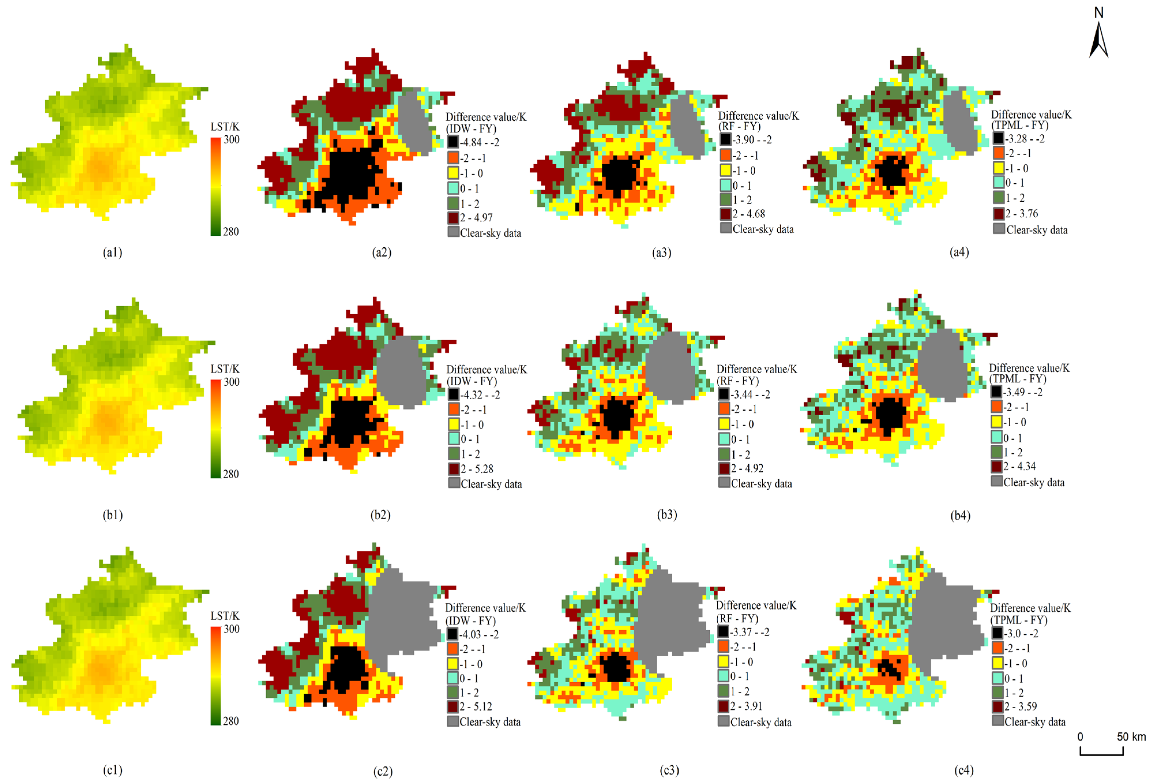
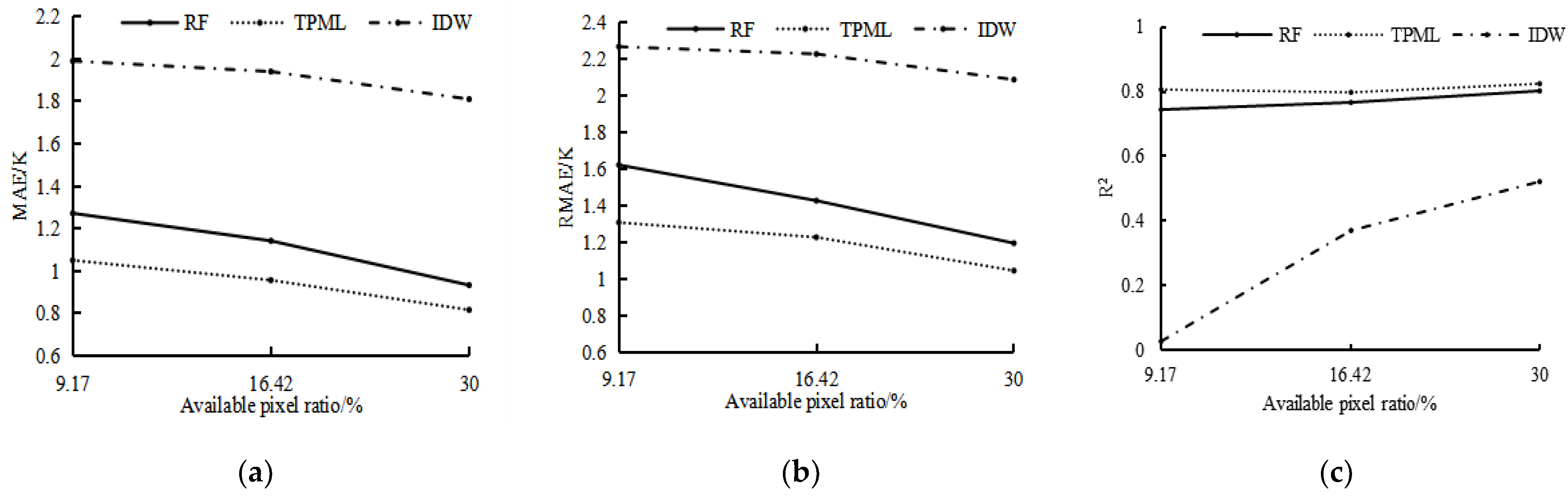
4.1.1. Results of Simulated Data Reconstruction

Figure 2 displays the difference maps between the reconstructed LST images and the original images using the IDW method, RF method, and TPML model. The pixels outside the grey areas on the spatial distribution map represent cloud-covered pixels. Comparing the LST difference maps of the three methods, it is evident that the IDW method has the poorest reconstruction results under different missing proportions. The maximum difference range for the IDW method is larger than that of the RF method and the TPML method, while the minimum difference value is smaller than that of the RF method and TPML method. Additionally, the area with the difference value greater than 2 K is significantly larger for the IDW method compared to the RF method and TPML method. The reconstructed results of the RF method and the TPML method are better, particularly for simulated image 3 with more missing data, as shown in Figure 2c3,c4. Moreover, the TPML method demonstrates higher accuracy in predicting higher land surface temperature. As the missing values increase, the reconstructed precision of the three methods become worse based on the illustration of Figure 2a3,a4,b3,b4, but it can be clearly seen that the reconstruction result of the TPML method is better than that of the RF method, and the number of pixels with larger differences is smaller, which has higher spatial consistency with the original LST image. In addition, according to the spatial distribution of the difference maps, the lack of high LST values in the simulated image resulted in LST underestimation in the region with relatively high temperature.

In terms of the quantitative indices, Figure 3 shows the MAE, RMSE, and R² between the original LST and the reconstruction results of the three methods. The effective pixel ratio in the horizontal coordinate of Figure 3 is the ratio of the number of clear-sky pixels to the total number of pixels in the study area. As can be seen from Figure 3, the IDW method has the largest MAE and RMSE and the smallest R², while the TPML method has the smallest MAE and RMSE and the largest R². With the increase in the effective pixel ratio, the RMSE, MAE, and R² differences between the RF and the TPML method gradually become smaller, but the reconstructed accuracy of the RF method is obviously poorer than that of the TPML method after the missing value rate gradually increases.

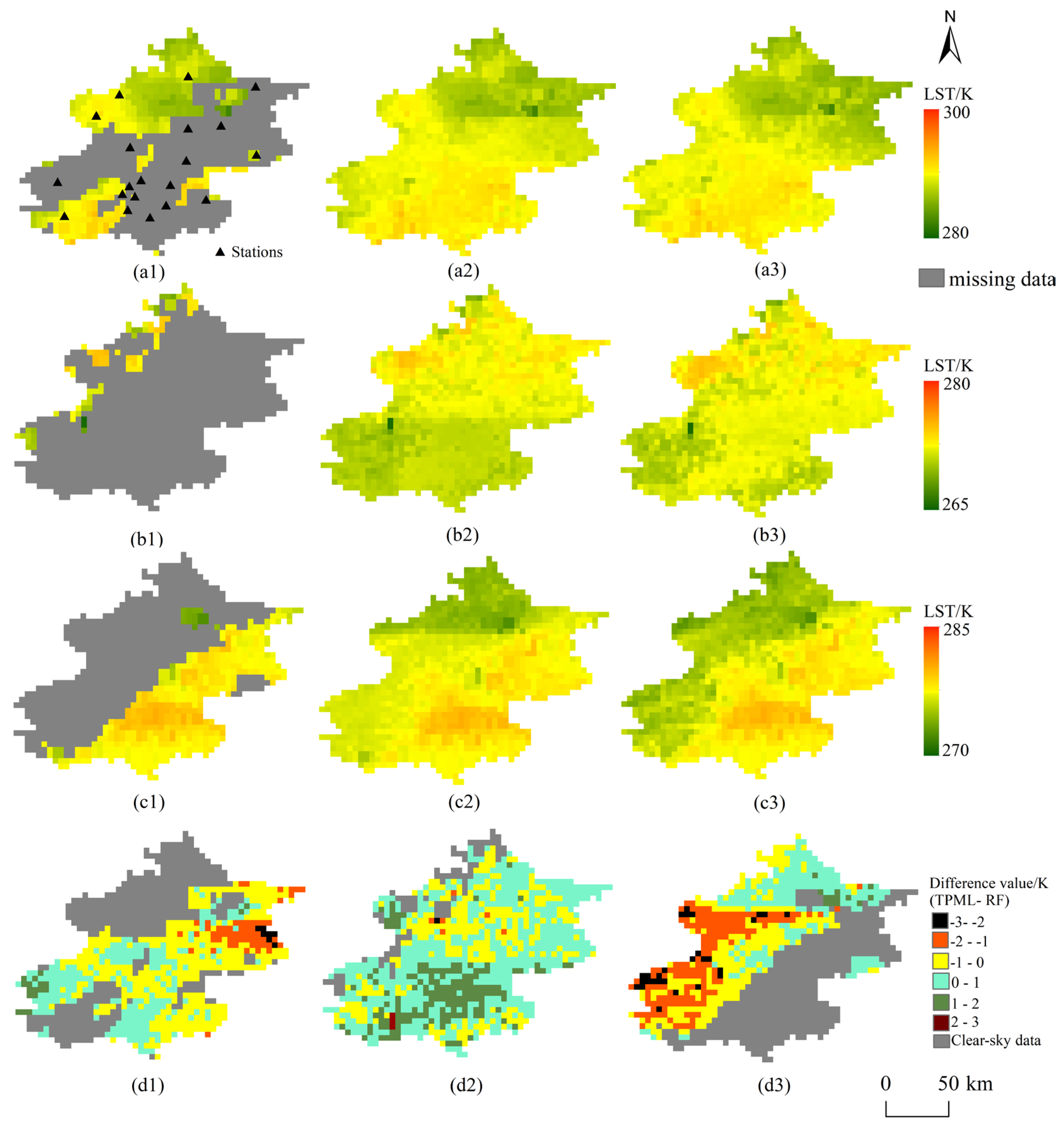
4.1.2. Actual Data Experiments and Results

(1)

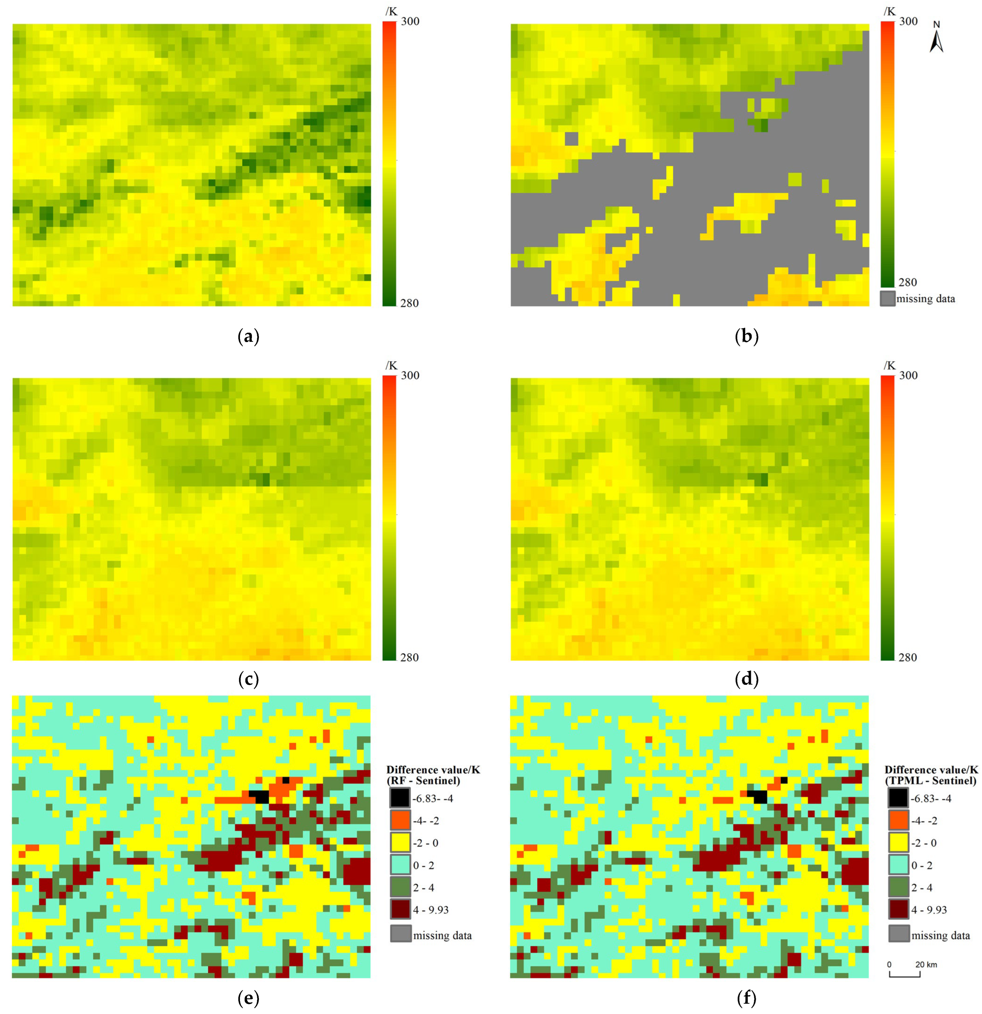
Reconstruction analysis of missing LST data

Taking 10:00 h on 1 October, 21:00 h on 6 October, and 06:00 h on 7 October 2021 as examples, the missing LST proportions were 60.55%, 91.65%, and 58.44%, respectively, and the missing LST data under theoretical clear-sky conditions were reconstructed using the RF and TPML methods. The results are shown in Figure 4. It can be seen that the spatial distribution characteristics of the reconstructed LST based on the two methods are similar. The LST spatial distribution reconstructed by the TPML method is more satisfactory than that of the RF method under different missing data proportions, and the reconstructed LST data preserve finer texture and spatial difference features, which can more accurately depict the LST spatial distribution pattern. With the increase in the number of missing pixels, as shown in Figure 4b2,b3, the spatial distribution of the reconstructed result by the RF method shows a significant fluctuation, which is obviously unreasonable, while the spatial distribution of the reconstructed LST data by the TPML method is more reasonable in comparison. In addition, comparing Figure 4a2,a3 with Figure 4c2,c3, it can be seen that when the missing LST data are concentrated in a block-shaped pattern, the LST spatial distributions reconstructed by the two methods are different, and the spatial texture features reconstructed by the RF method are very rough, while the texture features of the TPML method are more detailed. When the missing LST data are more discrete block deletions, as in Figure 4a2,a3, the difference between the LST spatial distribution reconstructed by the RF method and the TPML method is small, and the texture features do not differ too much.

Based on Figure 4d1–d3, it can be seen that the RF method and the TPML method exhibit some reconstruction differences. From Figure 4d1, it is evident that the pixels with larger differences of −2~−1 K between the two methods are primarily located in the eastern part of the study area, where the reconstructed results of the RF method exhibit unreasonable LST fluctuations. As for Figure 4d2, the TPML method yields higher reconstructed LST values than the RF method. The pixels with larger differences of 1~2 K are mainly distributed in the southern part of the study area. The largest difference between these two methods is illustrated in Figure 4d3; the RF method yields higher reconstructed LST values and many pixel values range from −2~−1 K, primarily distributed in the western part of the study area.

(2)

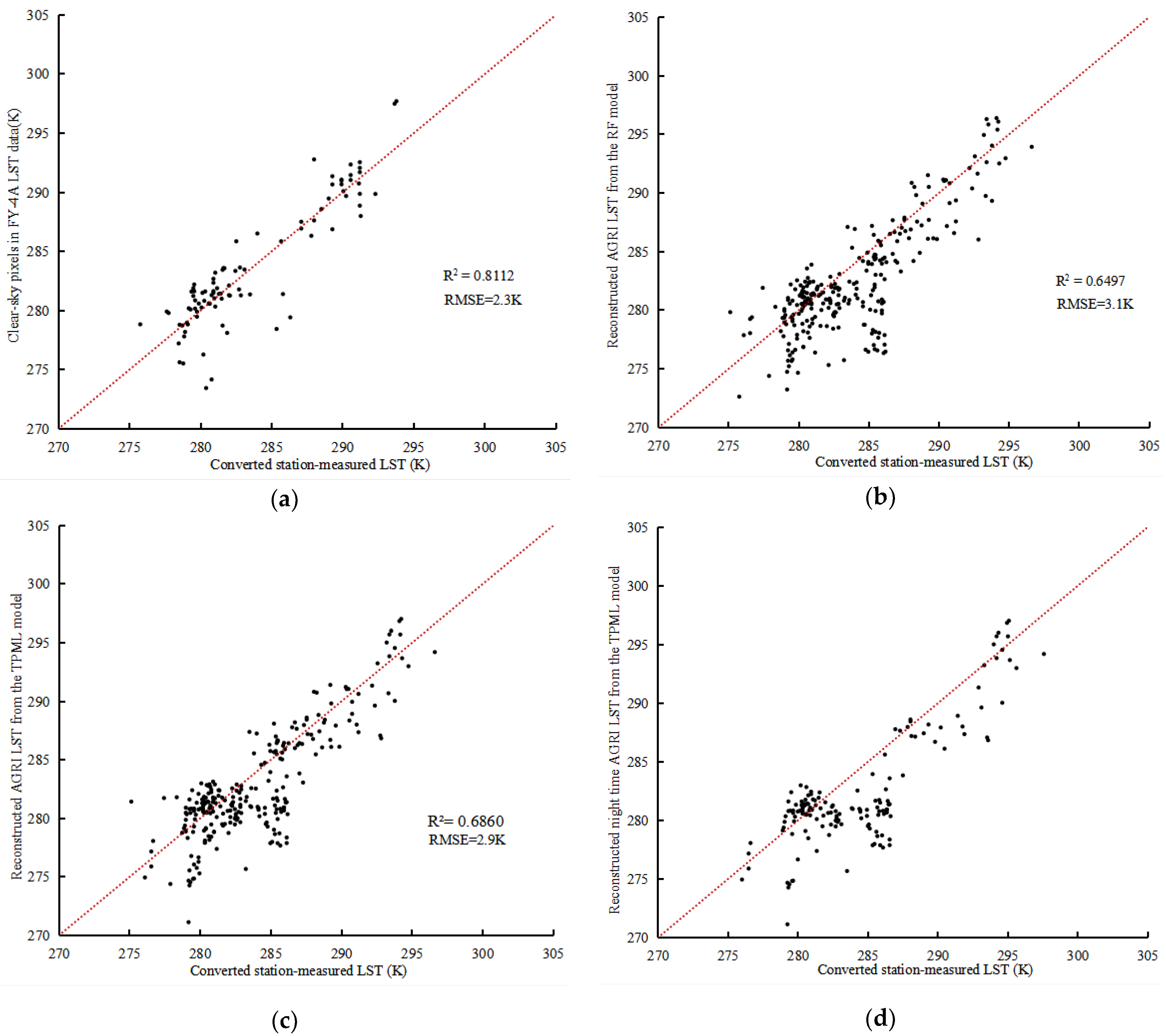
Accuracy assessment of the reconstructed results using station-measured LST data

In the actual data experiment, LST data from 18 different dates and times in October 2021 were selected as experimental data, and station-measured LST data in the study area from 20 meteorological stations were used to verify the LST reconstruction result from the RF method and TPML method. The locations of meteorological stations in the study area are shown in Figure 4a1. According to the effectiveness of the AGRI LST corresponding to the locations of the meteorological stations, we can determine if the station-measured LST is affected by clouds. The station-measured LSTs after scale correction under clear-sky conditions are directly compared with the FY-4A AGRI LST. The station-measured LSTs under clouds are used to evaluate the accuracy of the reconstructed AGRI LST. Because the limited number of validation sites and the data from a single time instance are insufficient for validation purposes, 18 times series of field-measured LST data were used together for accuracy assessment. Before validating the reconstruction results using station-measured LST, a scale-matching relationship between the station-measured data and AGRI LST under clear-sky conditions was established as shown in Equations (10) and (11). The RMSEs and MAEs before and after the scale conversion are 3.2 K/2.3 K and 4.3 K/1.6 K, respectively, which indicates that the station-observed LST after the conversion is much closer to the FY-4A AGRI LST, and the converted station-measured LST can be used to evaluate the reconstruction results of FY-4A AGRI LST in a more reliable way.

The number of clear-sky pixels and missing pixels at the station locations in the FY-4A AGRI LST data are 93 and 267, respectively. The AGRI LST of the clear-sky pixels and the reconstructed LST of the missing pixels are extracted according to the longitude and latitude of the ground stations, which are then compared with the field-measured LST after scale correction; the results are shown in Figure 5. From Figure 5, the clear-sky FY-4A AGRI LST data show a good correlation with the station-measured LST, with R² of 0.8112 and RMSE of 2.3 K. The R² between the reconstructed LST for missing pixels of the RF method and the station-measured LST is 0.6497, and the RMSE is 3.1 K; the R² and RMSE of the TPML method are 0.6860 and 2.9 K, and the reconstruction accuracy of the TPML method is higher than that of the RF method. Comparing the scatter diagrams between clear-sky and cloudy conditions, the correlation between the reconstructed LST and the station-measured LST is reduced, probably because the reconstructed LST of the missing pixels is estimated under theoretical clear-sky conditions rather than the actual LST under cloud cover. In addition, according to Figure 5c, some of the estimated LST of the missing pixels under the theoretical clear-sky conditions is lower compared with the station-measured LST, possibly because some of the selected FY-4A AGRI LST data are collected at night. The ground dissipates heat through thermal radiation at night, the atmosphere warms the ground in the form of inverse radiation, and the insulation effect of the atmosphere is more obvious when the cloud cover is thick. The LST cooling rate is slower under cloudy conditions compared to that under clear-sky conditions, so the station-measured LST is higher than the reconstructed LST under theoretical clear-sky conditions. Figure 5d presents the scatter diagram of the reconstructed time series of FY-4A AGRI LST for missing data with the measured LST at nighttime; it can be seen that the predicted LST under theoretical clear-sky conditions is smaller than the station-measured LST for most of the nighttime hours.

(3)

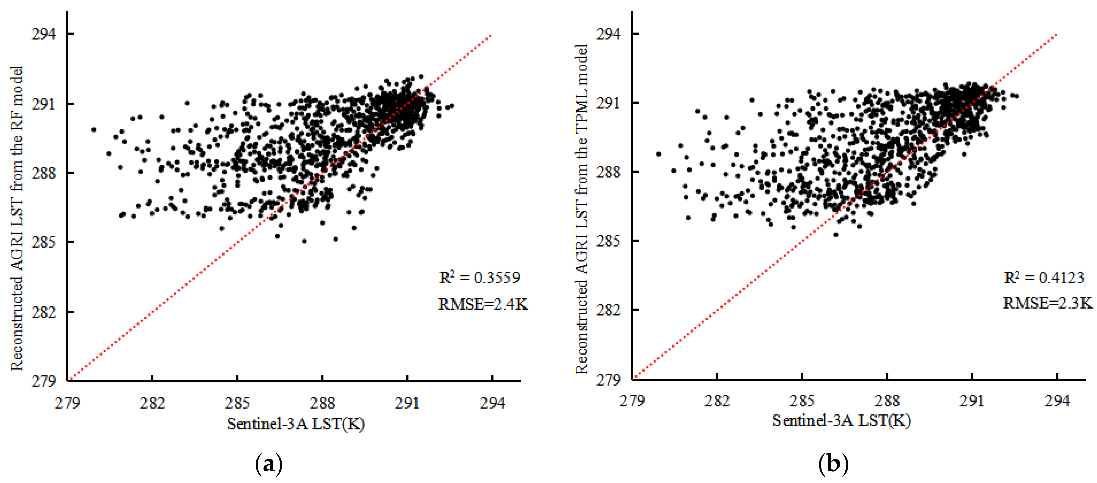
Accuracy assessment using Sentinel-3A LST data

Due to the complexity of land surface cover types in the study area, there are multiple landcover types in one AGRI pixel, while the ground stations observation corresponds to the LST of a small local area. Although the scale-conversion process is performed for the station-measured LST data, there are still some shortcomings in the accuracy assessment of the reconstruction results using the station-measured LST data. In this study, the Sentinel-3A LST data at the quasi-synchronous time are further used as the reference to evaluate the reconstruction accuracy of the two methods.

Differences between the FY-4A AGRI LST data and the Sentinel-3A LST data include imaging time of 21 min and satellite zenith angle of 15°. To make the comparable comparison between LST data from different sources, the FY-4A AGRI LST is used as the reference, and Equation (9) is used to make a linear correction for the Sentinel-3A LST to eliminate the difference between the FY-4A AGRI LST and the Sentinel-3A LST as much as possible. As shown in Figure 6, the RMSE and MAE of the Sentinel-3A LST data before and after the correction are 5.2 K, 1.3 K and 4.9 K, 0.92 K, respectively, which indicates that the difference between the corrected Sentinel-3A LST and the FY-4A AGRI LST is significantly smaller, and the two LST datasets are closer to each other. These analyses indicate that it is more reasonable to use the corrected Sentinel-3A LST to evaluate the reconstructed AGRI LST.

Taking the FY-4A AGRI LST data with an imaging time of 10:00 h Beijing time on 1 October 2021 as an example, the linear corrected Sentinel-3A LST image using Equation (9) and the AGRI LST image before and after the reconstruction are given in Figure 7. According to Figure 7a,b, the comparison between original FY-4A AGRI LST data and the corrected Sentinel-3A LST data shows that the LST spatial distribution of the two datasets is relatively close. Figure 7e and 7f respectively show the difference images between the reconstructed LST by the RF, TPML method and the linear revised Sentinel-3A LST, from which it can be seen that the difference under clear-sky conditions is almost within the range of −2 to 2 K. Therefore, it is possible to use the Sentinel-3A LST image as the reference to evaluate the reconstructed LST. Comparing Figure 7a,c,d, the distributions of high and low temperature in the reconstructed images of the two methods are similar to those of the Sentinel-3A LST image, and the reconstructed image by the RF method shows an obvious uneven LST distribution in one-third of the distance from the upper boundary of the image, while the reconstructed LST image by the TPML method shows a uniform distribution without any unreasonable temperature jumps, which shows that the TPML method is better than the RF method. By comparing Figure 7e,d, it can be clearly seen that in the upper right corner of the reconstructed LST image, the number of pixels with differences in the range of −4~−2 K and 2~4 K for the RF method is more than that of the TPML method, which indicates that the TPML method has a higher accuracy in the reconstruction of the LST under cloud cover.

In terms of the quantitative indices, as shown in Figure 8a,b, the R² between the reconstructed results of the RF method and the reference data is 0.3559, and the RMSE is 2.4 K. The R² between the reconstruction results of the TPML method and the reference data is 0.4123, and the RMSE is 2.3 K. Overall, the reconstructed accuracy of the RF method is lower than that of the TPML method.

It should be noted that at 4 km spatial resolution, the missing LST pixels in the FY-4A AGRI data have normal LST values at the same location in the Sentinel-3A data, mainly because the difference in the original spatial resolution between the two sensors is large, and the LST cannot be effectively retrieved when there are partial clouds in one AGRI pixel. The pixel with the missing LST in the FY4A AGRI data includes 16 Sentinel-3A pixels, while most of Sentinel-3A pixels may be under clear-sky conditions. In addition, because there is a 21-min difference between the FY-4A AGRI LST data and the Sentinel-3A LST data, the LST may also vary considerably, and direct comparison of these two data will also be subject to error.

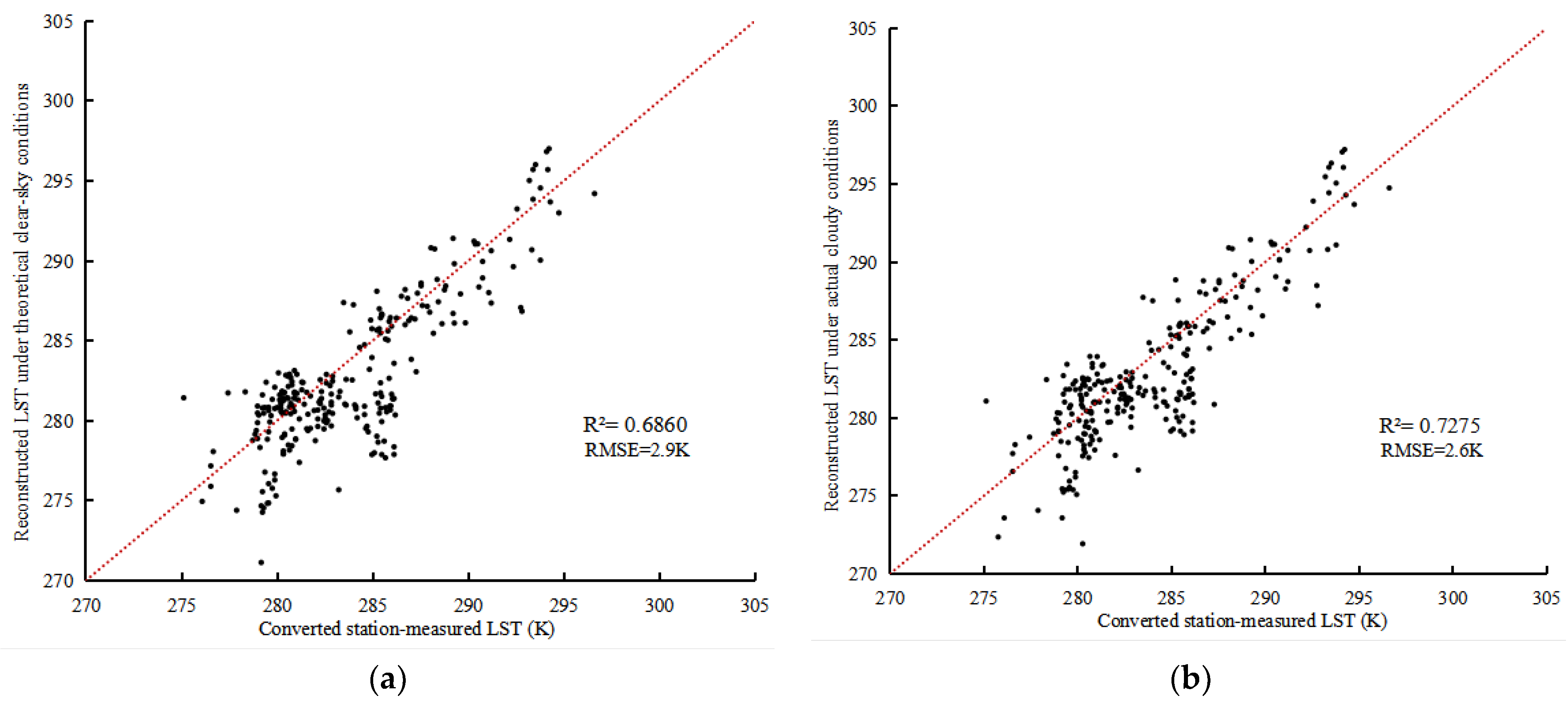
4.2. Analysis of Actual LST Reconstruction Results under Cloudy Conditions

A model is established using the FY-4A LST data under clear-sky conditions with the ERA5 LST data in the same area and at the same time, and then the ERA5 LST data are revised based on this model. Taking the imaging time of 10:00 h Beijing time on 1 October 2021 as an example, Figure 9 compares the ERA5 LST data before and after linear correction with the FY-4A LST data. We find that the corrected ERA5 LST data are closer to the FY-4A AGRI LST data, which is more reasonable for estimating the actual FY-4A LST under cloudy conditions.

According to the results of the simulated experiments and actual experiments, the reconstructed accuracy of the TPML method is better than that of the RF method, so the reconstructed LST under theoretical clear-sky conditions by the TPML method is chosen to reconstruct the actual LST under cloudy conditions, then the accuracy of the recovered LST under theoretical clear-sky conditions and the actual LST under cloudy conditions is evaluated using the field-measured LST. Figure 10a shows a scatter diagram comparing the station-measured LST and the estimated LST under the theoretical clear-sky conditions, with an R² of 0.6860 and RMSE of 2.9 K. Figure 10b shows a scatter diagram comparing the station-measured LST and the actual LST under cloudy conditions, with an R² of 0.7275 and RMSE of 2.6 K. The RMSE of the reconstructed actual LST is 10.34% lower than that of the theoretical clear-sky LST, which indicates that the LST reconstruction results under the theoretical clear-sky conditions need to be further reconstructed to obtain the actual LST under cloudy conditions. According to Figure 10a,b, the measured LST is high at most ground stations, which may be caused by the following factors: (1) the station-measured LST is collected within flat bare ground, and the LST of bare ground is generally higher than other surface types during daytime, while the FY-4A LST data are mostly for mixed pixels, and the LST at the pixel scale is the non-isothermal temperature of multiple surface types; (2) due to the absence of high LST in the FY-4A LST data in 18 instances, the phenomenon of low reconstructed values of higher-temperature pixels may arise.

In this paper, the reconstructed LST is compared with the simulated LST, Sentinel-3A LST, ERA5 LST, and the measured LST; it can be found that each of these LST used for the accuracy comparison analysis has its own advantages and disadvantages, which are summarized in

Table 3. Summary of the performances of different validation data.

Validation Data	Positives	Limitations
Simulated LST	Can be used to accurately compare reconstruction precision between different methods and has no relation with imaging time, spatial resolution, and sensor observation angle.	Accuracy can only be evaluated in simulated experiments.
Sentinel-3A LST	The LST reconstruction results can be quantitatively evaluated in actual experiments at the scale of spatial distribution.	Inconsistency between observation angle, imaging time, spatial resolution and LST retrieval methods for Sentinel and FY-4A sensors.
ERA5 LST	ERA5 LST data are spatiotemporally continuous, which can match with FY AGRI data well from the point of view of time.	Uncertain LST accuracy for various land cover types, and large difference in spatial resolution between ERA5 data and FY data.
Ground station LST	Long time and continuous data acquisition, high LST accuracy.	Spatial scale between station ‘point’ measurements and sensor ‘grid’ observations; limited number of stations in the study area.

.

5. Conclusions

This study mainly investigates the relationship between the FY-4A AGRI LST data and auxiliary variables to establish a TPML model to reconstruct missing LST data, which is compared with the RF method. The research results demonstrate that the reconstructed LST from the TPML method exhibit a more accurate spatial distribution and detailed texture information. In actual data experiments, the R² and RMSE of the TPML method are 0.6860 and 2.9 K, respectively, which are significantly more accurate than those of the RF method. Furthermore, by using ERA5 LST as the auxiliary data, the reconstructed LST under cloudy conditions yields R² and RMSE values of 0.7275 and 2.6 K, respectively, with a 10.34% decrease in RMSE compared to theoretical clear-sky conditions. This indicates that the actual LST reconstruction results can be obtained with the help of ERA5 LST data based on the reconstructed theoretical clear-sky LST. The proposed method in this paper can be further improved by replacing the ERA5 LST data with other LST data with higher accuracy.

The TPML model effectively integrates the auxiliary variables and its location information, and utilizes the spatial correlation of each image element and attribute similarity to improve the prediction accuracy. The model is not only applicable to predict LST distribution but also to estimate other environmental variables that exhibit spatial correlation and have abundant auxiliary data. In the future, the RF in the TPML model can be replaced with other machine learning methods to further improve prediction accuracy.

However, this research has some limitations that require further analysis: (1) the TPML model is more computationally intensive compared to the RF method and consumes more time when reconstructing large regions. The TPML method needs to calculate the differences in clear-sky LST and its auxiliary variables of paired points before modeling, the number of input variables becomes square times of that of the original quantity, which results in the TPML modeling process taking a longer time. When applying the model to cloud-affected pixels, the variable differences between the clear-sky and cloudy pixels also need more computation time and occupy more memory resources. (2) This research attempts to assess the accuracy of the reconstructed LST results using data from different sources, but there are some uncertainties and differences in the satellite-derived “grid data”, field-measured “point data”, and model-simulated “reanalyzed data”, and it is not easy to carry out cross-validation of the LST reconstruction results under the influence of clouds by using other optical remotely sensed imagery as a reference.

References

1. Hansen, J.; Ruedy, R.; Sato, M.; Lo, K. Global surface temperature change. Rev. Geophys. 2010, 48, 1–29. [Google Scholar]
2. Anderson, M.C.; Allen, R.G.; Morse, A.; Kustas, W.P. Use of Landsat thermal imagery in monitoring evapotranspiration and managing water resources. Remote Sens. Environ. 2012, 122, 50–65. [Google Scholar]
3. Jia, Y.Y.; Li, Z.L. Progress in land surface temperature retrieval from passive microwave remotely sensed data. Prog. Geogr. 2006, 25, 96–105. [Google Scholar]
4. Tu, L.L.; Qin, Z.H.; Zhang, J.; Liu, M.; Geng, J. Estimation and error analysis of land surface temperature under the cloud based on spatial interpolation. Remote Sens. Inf. 2011, 4, 59–63. [Google Scholar]
5. Lu, L.; Venus, V.; Skidmore, A.; Wang, T.; Luo, G. Estimating land-surface temperature under clouds using MSG/SEVIRI observations. Int. J. Appl. Earth Obs. Geoinf. 2011, 13, 265–276. [Google Scholar]
6. Neteler, M. Estimating daily land surface temperatures in mountainous environments by reconstructed MODIS LST data. Remote Sens. 2010, 2, 333–351. [Google Scholar]
7. Zeng, C.; Long, D.; Shen, H.; Wu, P.; Cui, Y.; Hong, Y. A two-step framework for reconstructing remotely sensed land surface temperatures contaminated by cloud. ISPRS J. Photogramm. Remote Sens. 2018, 141, 30–45. [Google Scholar]
8. Xu, Y.; Shen, Y. 2013. Reconstruction of the land surface temperature time series using harmonic analysis. Comput. Geosci. 2013, 61, 126–132. [Google Scholar]
9. Liu, Z.; Wu, P.; Duan, S.; Zhan, W.; Ma, X.; Wu, Y. Spatiotemporal reconstruction of land surface temperature derived from fengyun geostationary satellite data. IEEE J. Sel. Top. Appl. Earth Obs. Remote Sens. 2017, 10, 4531–4543. [Google Scholar] [CrossRef]
10. Weiss, D.J.; Mappin, B.; Dalrymple, U.; Bhatt, S.; Cameron, E.; Hay, S.I.; Gething, P.W. Re-examining environmental correlates of Plasmodium falciparum malaria endemicity: A data-intensive variable selection approach. Malar. J. 2015, 14, 68. [Google Scholar] [CrossRef]
11. Liu, Z.; Wu, P.; Wu, Y.; Shen, H.; Zeng, C. Robust reconstruction of missing data in Feng Yun geostationary satellite land surface temperature products. J. Remote Sens. 2017, 21, 40–51. [Google Scholar] [CrossRef]
12. Zhang, J.; Qin, Z.H.; Liu, M.; Tu, L.L.; Zhou, Y.; Yang, Q. Estimating of land surface temperature under the cloud cover with spatial interpolation. Geogr. Geo-Inf. Sci. 2011, 27, 45–49. [Google Scholar]
13. Liu, M. Study on Estimation of LST under Cloudy Region in MODIS Images. Master’s Thesis, Nanjing University, Nanjing, China, 2012. [Google Scholar]
14. Wu, P.; Yin, Z.; Yang, H.; Wu, Y.; Ma, X. Reconstructing geostationary satellite land surface temperature imagery based on a multiscale feature connected convolutional neural network. Remote Sens. 2019, 11, 300. [Google Scholar] [CrossRef]
15. Ke, L.; Ding, X.; Song, C. Reconstruction of time-series MODIS LST in Central Qinghai-Tibet Plateau using geostatistical approach. IEEE Geosci. Remote Sens. Lett. 2013, 10, 1602–1606. [Google Scholar] [CrossRef]
16. Zhao, W.; Duan, S.B. Reconstruction of daytime land surface temperatures under cloud-covered conditions using integrated MODIS/Terra land products and MSG geostationary satellite data. Remote Sens. Environ. 2020, 247, 111931. [Google Scholar] [CrossRef]
17. Wu, D. Land Surface Temperature Reconstruction Based on FY-2F Geostationary Meteorological Satellite Data. Master’s Thesis, Nanjing University of Information Science and Technology, Nanjing, China, 2018. [Google Scholar]
18. Gao, B.; Stein, A.; Wang, J. A two-point machine learning method for the spatial prediction of soil pollution. Int. J. Appl. Earth Obs. Geoinf. 2022, 108, 102742. [Google Scholar] [CrossRef]
19. Wang, Q.P.; Wu, X.J.; Chen, Y.Q.; Duan, J. Visualization and Application of FY-4A Satellite Data. Meteorol. Sci. Technol. 2019, 47, 502–507. [Google Scholar]
20. Zhang, Z.Q.; Dong, Y.H.; Ding, L.; Wang, G.; Fang, X.; Zhang, X.; Huang, F. China’s first second-generation FY-4 meteorological satellite launched. Space Int. 2016, 12, 6–12. [Google Scholar]
21. Zhang, P.; Guo, Q.; Chen, B.Y.; Feng, X. The Chinese next-generation geostationary meteorological satellite FY-4 compared with the Japanese Himawari-8/9 satellites. Adv. Meteorol. Sci. Technol. 2016, 6, 72–75. [Google Scholar]
22. Li, X.; Zhang, G.; Zhu, S.; Xu, Y. Step-By-Step Downscaling of Land Surface Temperature Considering Urban Spatial Morphological Parameters. Remote Sens. 2022, 14, 3038. [Google Scholar] [CrossRef]
23. Zhu, J.H.; Zhu, S.Y.; Yu, F.C.; Zhang, G.X.; Xu, Y.M. A downscaling method for ER A5 reanalysis land surface temperature over urban and mountain areas. Natl. Remote Sens. Bull. 2021, 25, 1778–1791. [Google Scholar] [CrossRef]
24. Zhang, G.; Wang, S.; Zhu, S.; Xu, Y. Spatial Distribution of High-temperature Risk with a Return Period of Different Years in the Yangtze River Delta Urban Agglomeration. Chin. Geogr. Sci. 2022, 32, 963–978. [Google Scholar] [CrossRef]
25. Pede, T.; Mountrakis, G. An empirical comparison of interpolation methods for MODIS 8-day land surface temperature composites across the conterminous Unites States. ISPRS J. Photogramm. Remote Sens. 2018, 142, 137–150. [Google Scholar] [CrossRef]
26. Sarafanov, M.; Kazakov, E.; Kalyuzhnaya, A.V. A Machine Learning Approach for Remote Sensing Data Gap-Filling with Open-Source Implementation: An Example Regarding Land Surface Temperature, Surface Albedo and NDVI. Remote Sens. 2020, 12, 3865. [Google Scholar] [CrossRef]
27. Breiman, L. Random forests. Mach. Learn. 2001, 45, 5–32. [Google Scholar] [CrossRef]
28. Jiang, G.M.; Liu, R. Retrieval of sea and land surface temperature from SVISSR/FY-2C/D/E measurements. IEEE Trans. Geosci. Remote Sens. 2014, 52, 6132–6140. [Google Scholar] [CrossRef]
29. Chen, D.H.; Zou, C.; Wang, S.Y.; Li, H.; Zhang, X.S. Study on spatial interpolation of the average temperature in the yili river valley based on dem. Spectrosc. Spectr. Anal. 2011, 31, 1925–1929. [Google Scholar]
30. Lin, Z.H.; Mo, X.Y.; Li, H.X.; Li, H.B. Comparison of three spatial interpolation methods for climate variables in china. Acta Geogr. Sin. 2002, 57, 47–56. [Google Scholar]
31. Long, D.; Yan, L.; Bai, L.; Zhang, C.; Shi, C. Generation of MODIS-like land surface temperatures under all-weather conditions based on a data fusion approach. Remote Sens. Environ. 2020, 246, 111863. [Google Scholar] [CrossRef]
32. Zhang, X.; Zhou, J.; Liang, S.; Chai, L.N.; Wang, D.D.; Liu, J. Estimation of 1-km all-weather remotely sensed land surface temperature based on reconstructed spatial-seamless satellite passive microwave brightness temperature and thermal infrared data. ISPRS J. Photogramm. Remote Sens. 2020, 167, 321–344. [Google Scholar] [CrossRef]
33. Muñoz-Sabater, J.; Dutra, E.; Agustí-Panareda, A.; Albergel, C.; Arduini, G.; Balsamo, G.; Boussetta, S.; Choulga, M.; Harrigan, S.; Hersbach, H.; et al. Era5-land: A state-of-the-art global reanalysis dataset for land applications. Earth Syst. Sci. Data 2021, 13, 4349–4383. [Google Scholar] [CrossRef]
Figure 1. Flowchart of this research.
Remotesensing 15 05179 g001
Figure 2. Difference maps between reconstructed LST images and original images. (a1c1) Original AGRI LST image; (a2c2) difference maps of IDW method for simulated image 1, simulated image 2, and simulated image 3; (a3c3) difference maps of RF method for simulated image 1, simulated image 2, and simulated image 3; (a4c4) difference maps of TPML method for simulated image 1, simulated image 2, and simulated image 3.
Remotesensing 15 05179 g002
Figure 3. Reconstruction accuracy of the three methods. (a) Curves of the MAEs; (b) curves of the RMSEs; (c) curves of R2.
Remotesensing 15 05179 g003
Figure 4. Reconstruction results of actual LST data using two methods. (a1c1) AGRI LST acquired at 10:00 h local time on 1 October, 21:00 h on 6 October, and 06:00 h on 7 October 2021. (a2c2) LST reconstructed by the RF method for three AGRI LST images. (a3c3) LST reconstructed by the TPML method. (d1d3) Difference distribution between TPML and RF reconstruction results for three AGRI LST images.
Remotesensing 15 05179 g004
Figure 5. Accuracy assessment of the reconstruction results of the two methods. (a) Clear-sky AGRI LST; (b) reconstructed LST by the RF method; (c) reconstructed LST by the TPML method; (d) reconstructed LST by the TPML method at night.
Remotesensing 15 05179 g005
Figure 6. Scatter diagrams of FY-4A AGRI LST versus Sentinel-3A LST before and after linear correction: (a) before correction; (b) after correction.
Remotesensing 15 05179 g006
Figure 7. Sentinel-3A LST and FY-4A LST before and after reconstruction. (a) Corrected Sentinel LST at 10:21 h on 1 October 2021; (b) FY-4A LST at 10:00 h on 1 October 2021; (c) RF reconstructed LST; (d) TPML reconstructed LST; (e) difference map between reconstructed LST by the RF method and revised Sentinel-3A LST; (f) difference map between reconstructed LST by the TPML method and revised Sentinel-3A LST.
Remotesensing 15 05179 g007
Figure 8. Correlation between the reconstructed FY-4A LST and the Sentinel-3A LST. (a) Reconstructed LST under theoretical clear-sky conditions by the RF method; (b) reconstructed LST under theoretical clear-sky conditions by the TPML method.
Remotesensing 15 05179 g008
Figure 9. Spatial distribution comparisons of ERA5 LST before and after correction with FY-4A AGRI LST data. (a) FY-4A LST; (b) ERA5 LST before correction; (c) ERA5 LST after correction.
Remotesensing 15 05179 g009
Figure 10. Correlation between the reconstructed LST under different conditions and the corrected station-measured LST. (a) Correlation between the reconstructed LST under theoretical clear-sky conditions and the station-measured LST; (b) correlation between the reconstructed LST under actual cloudy conditions and the station-measured LST.
Remotesensing 15 05179 g010