

Retrieval of Water Quality Parameters in Dianshan Lake Based on Sentinel-2 MSI Imagery and Machine Learning: Algorithm Evaluation and Spatiotemporal Change Research
 ,
,
Abstract
:1. Introduction
2. Materials and Methods
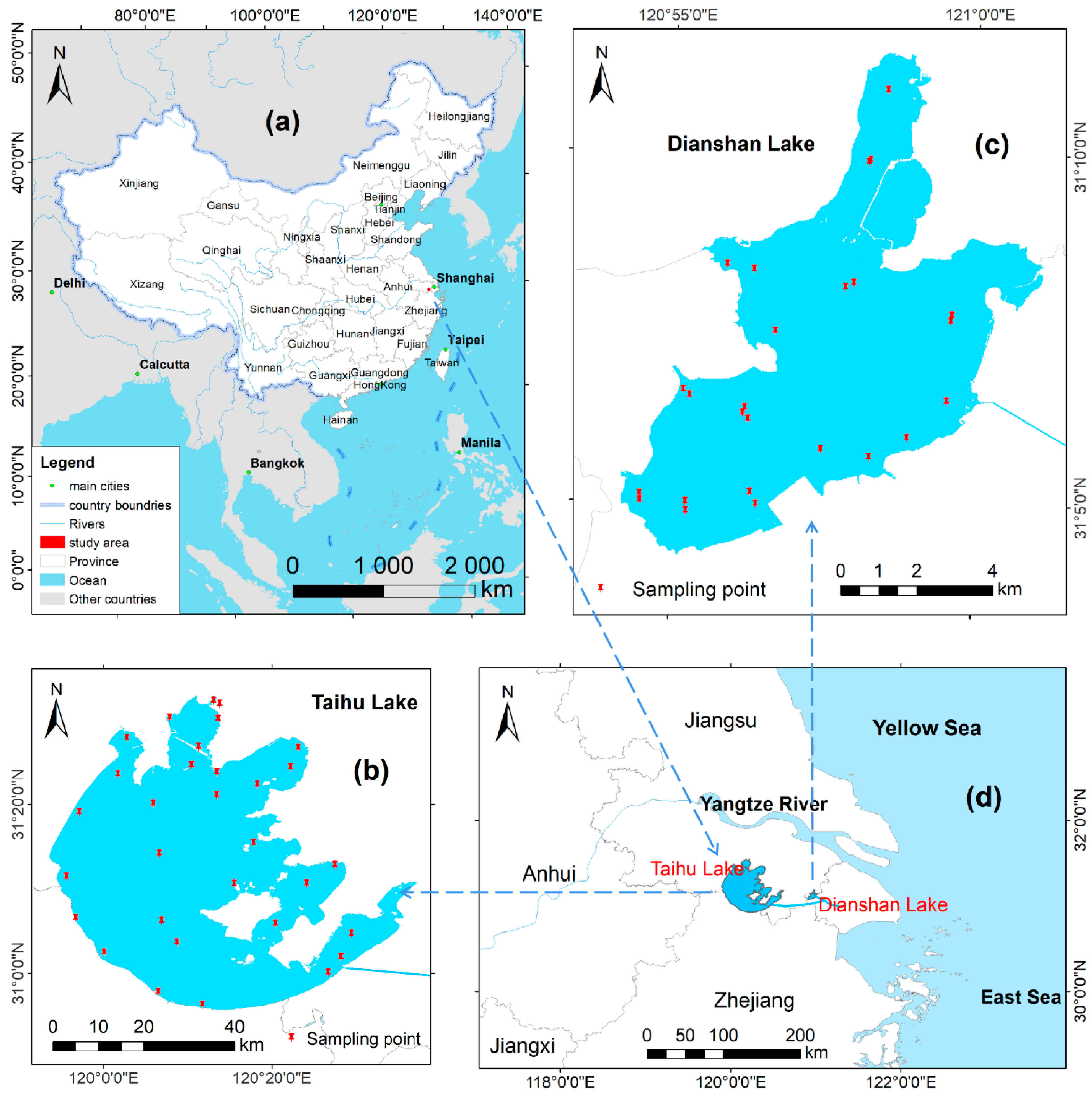
2.1. Study Area
2.2. Dataset
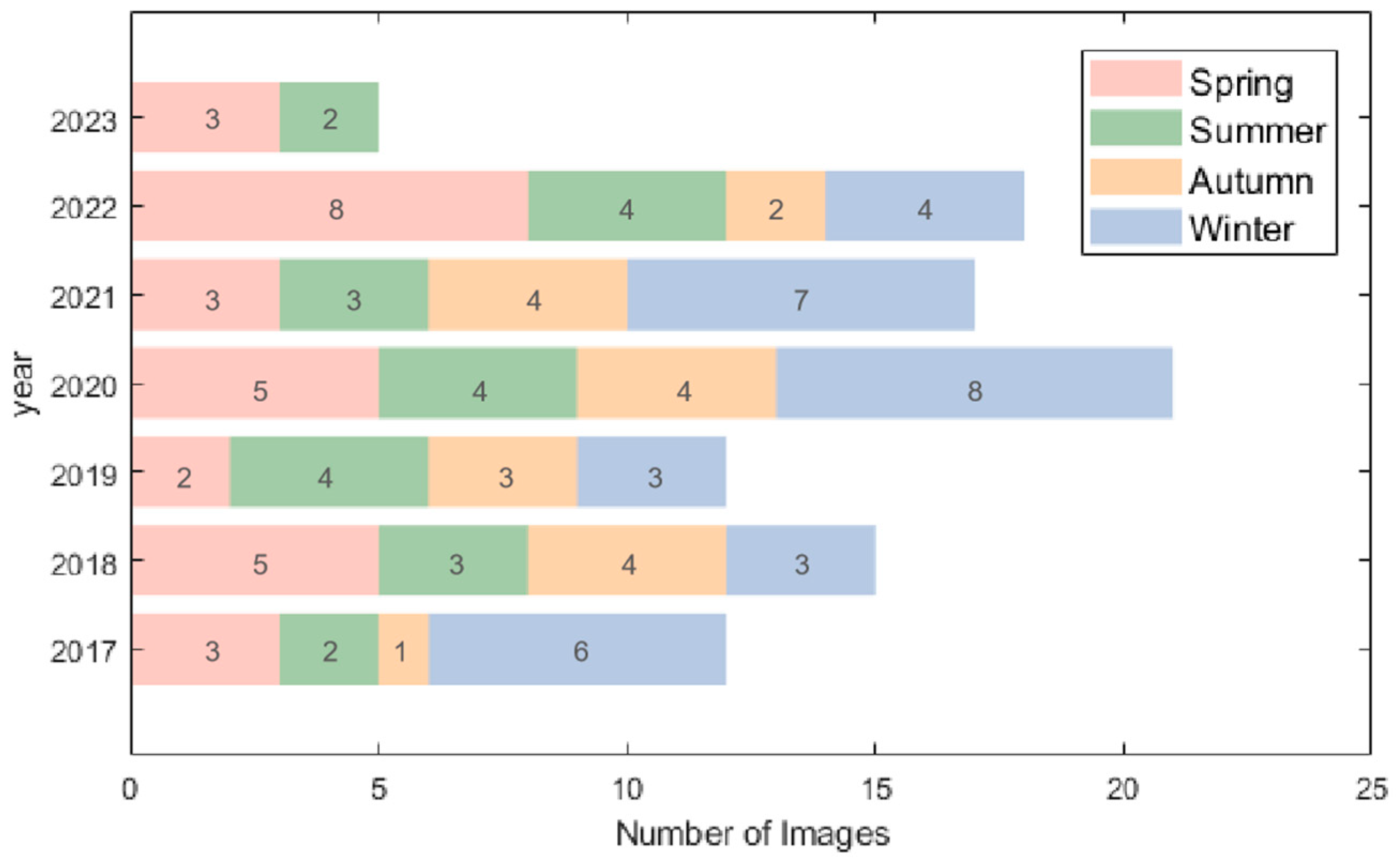
2.2.1. Satellite Data
2.2.2. Field Data
2.3. Modeling
2.4. Accuracy Evaluation
3. Results and Analysis
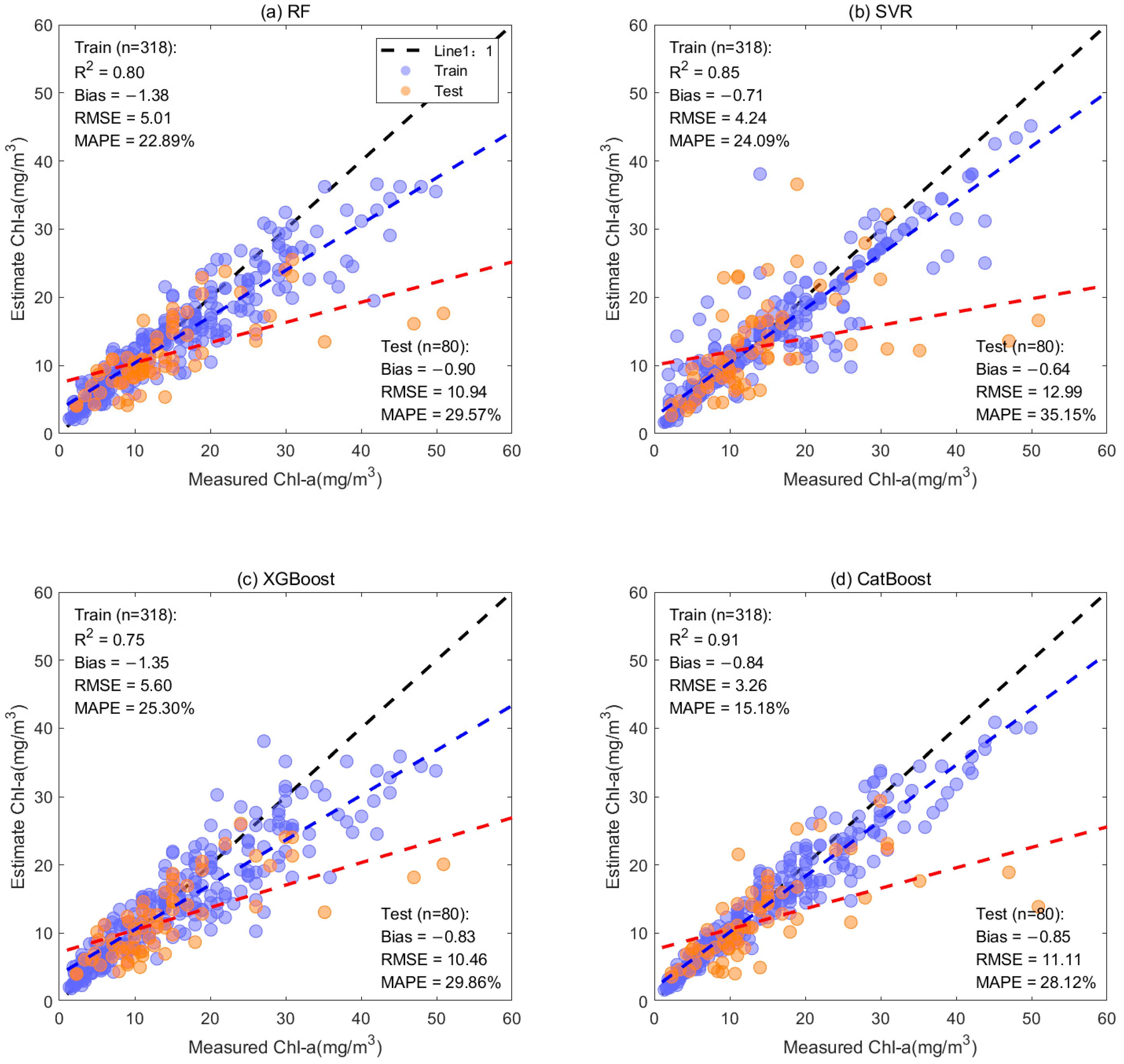
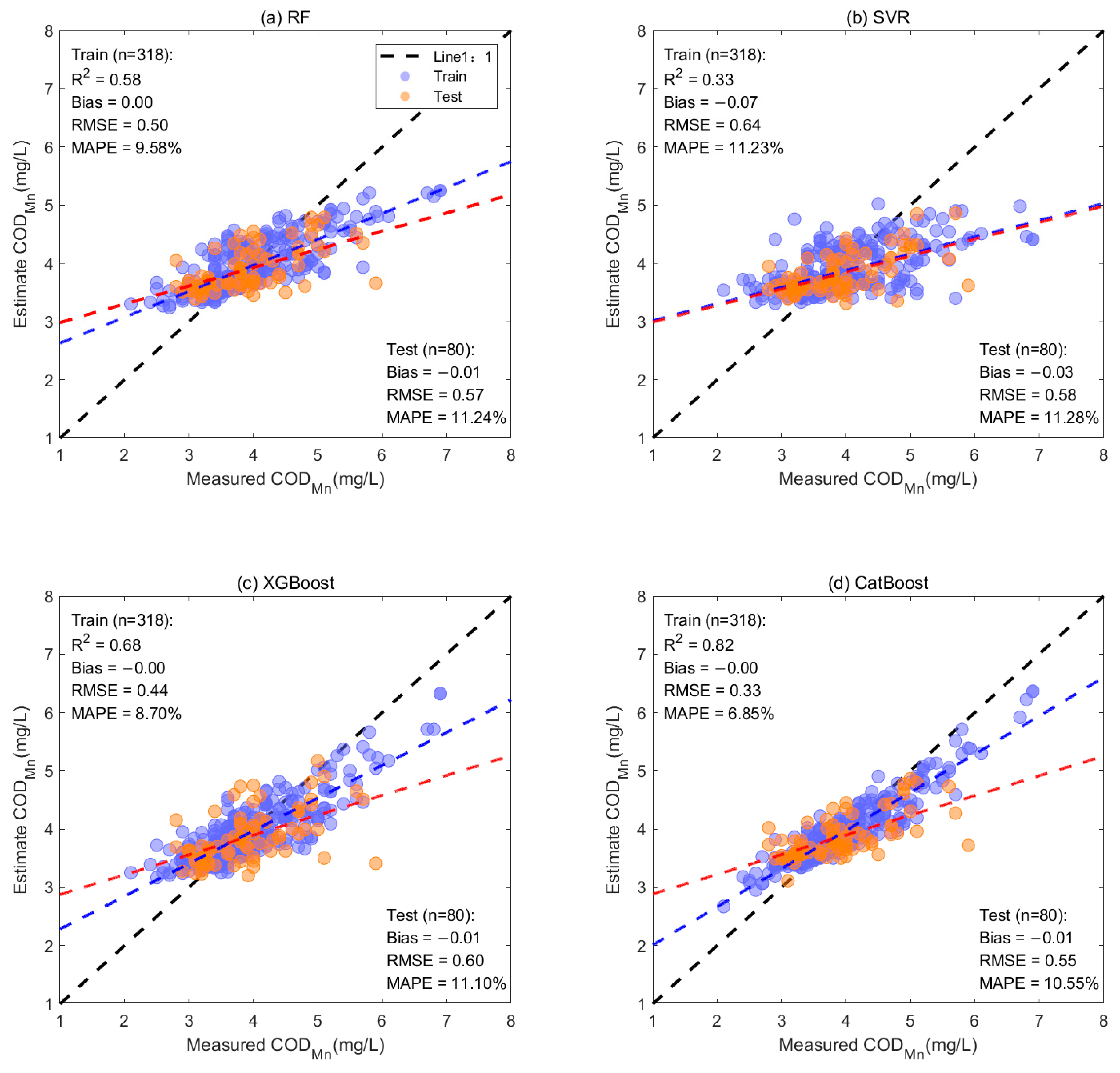
3.1. Model Calibration and Validation
3.2. Spatiotemporal Patterns of Diandao Lake Water Quality Based on Sentinel-2
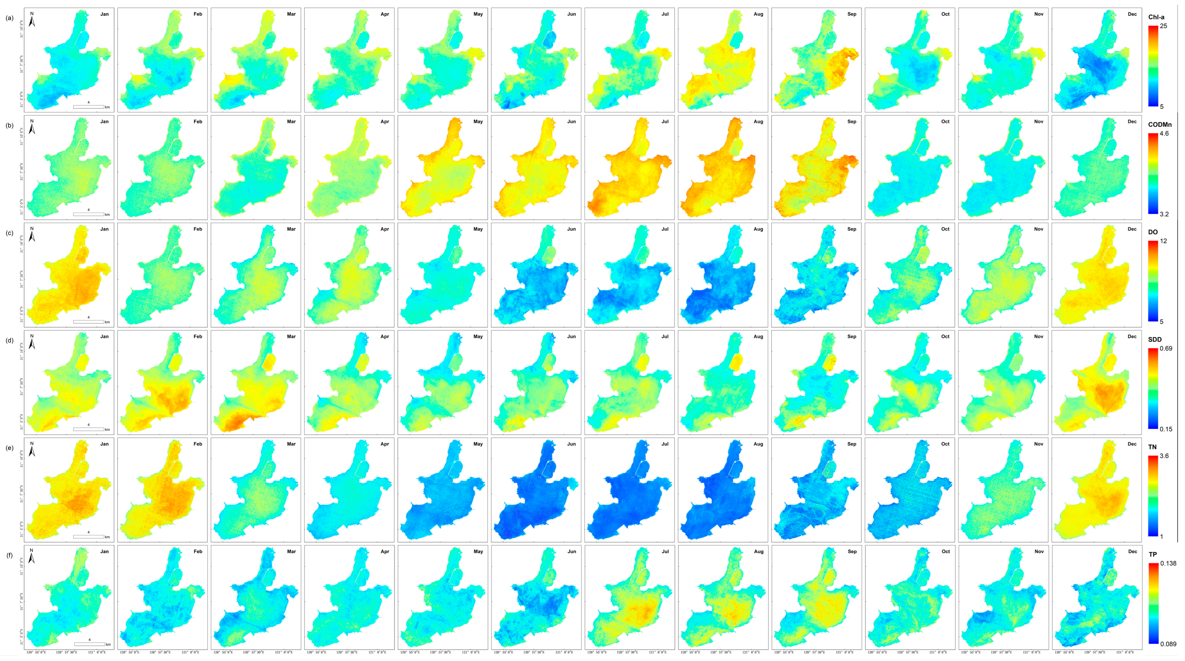
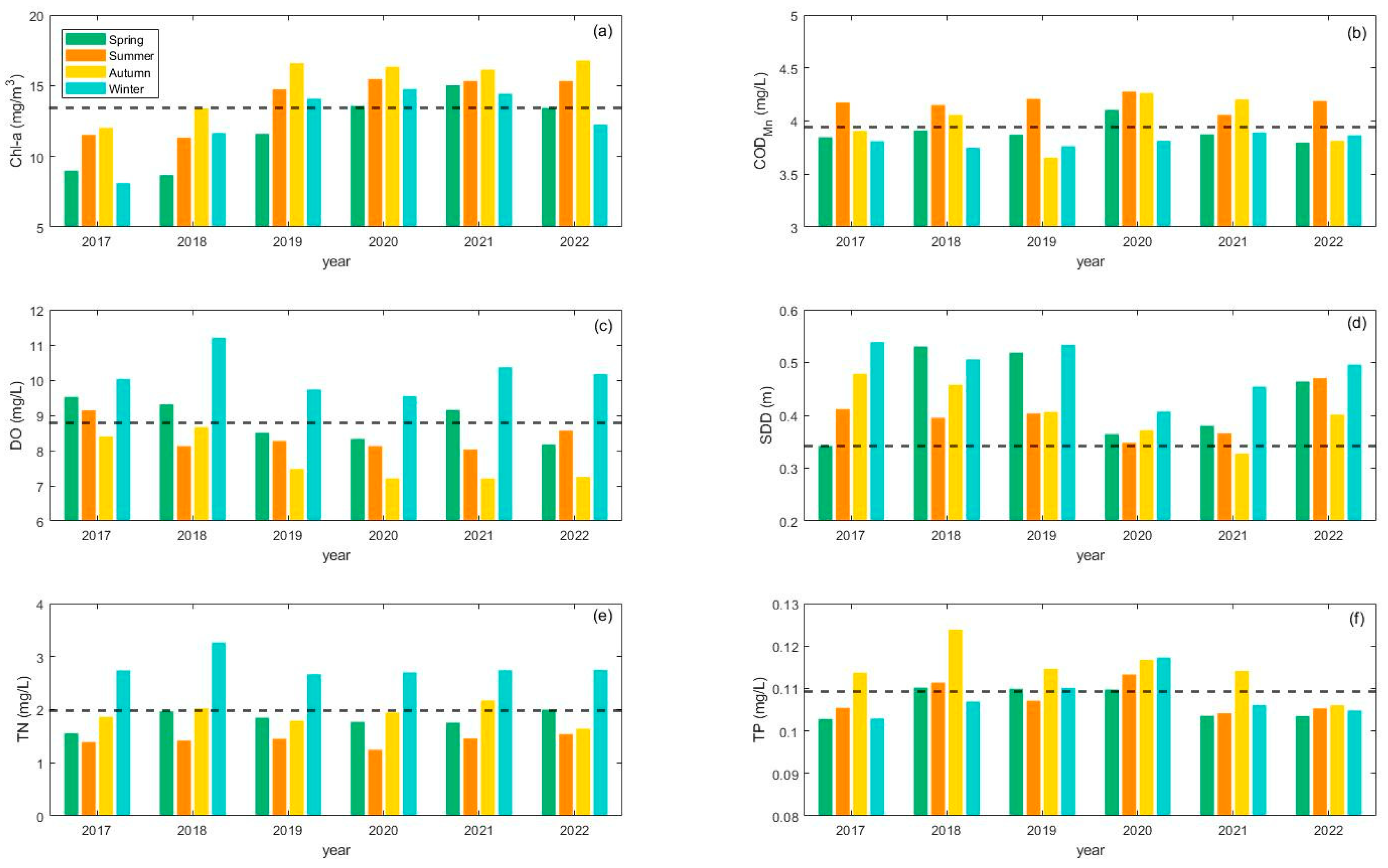
3.2.1. Temporal Variation
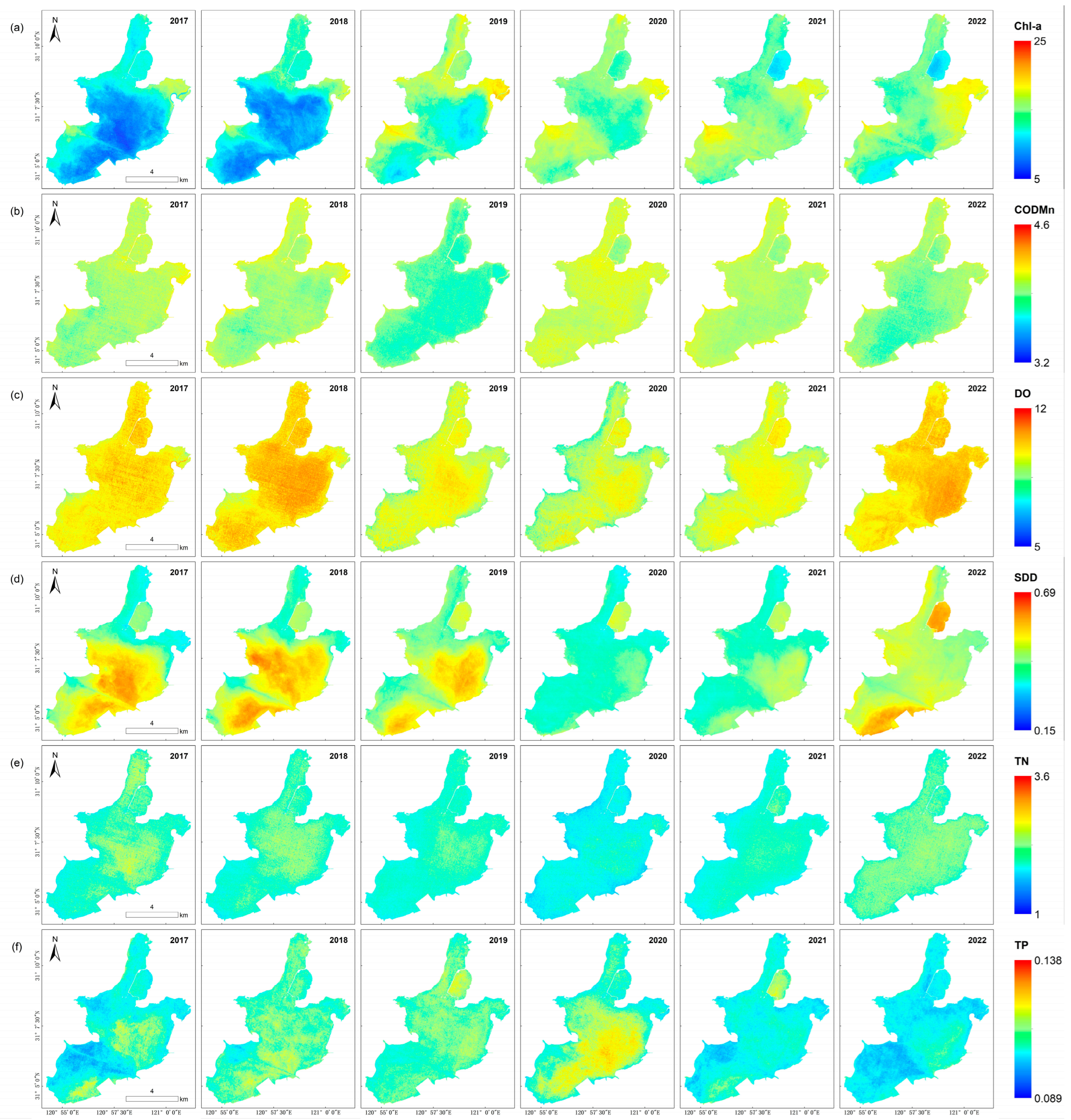
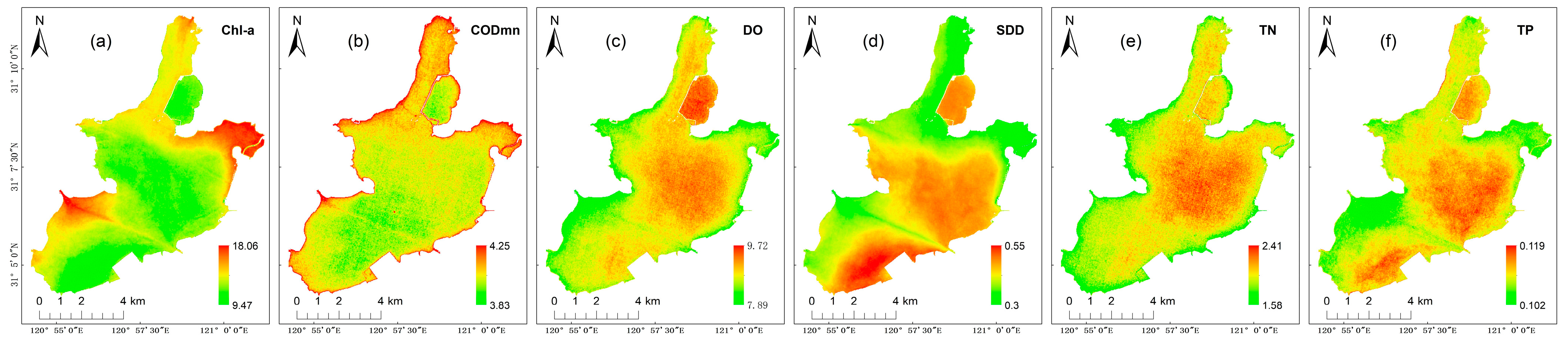
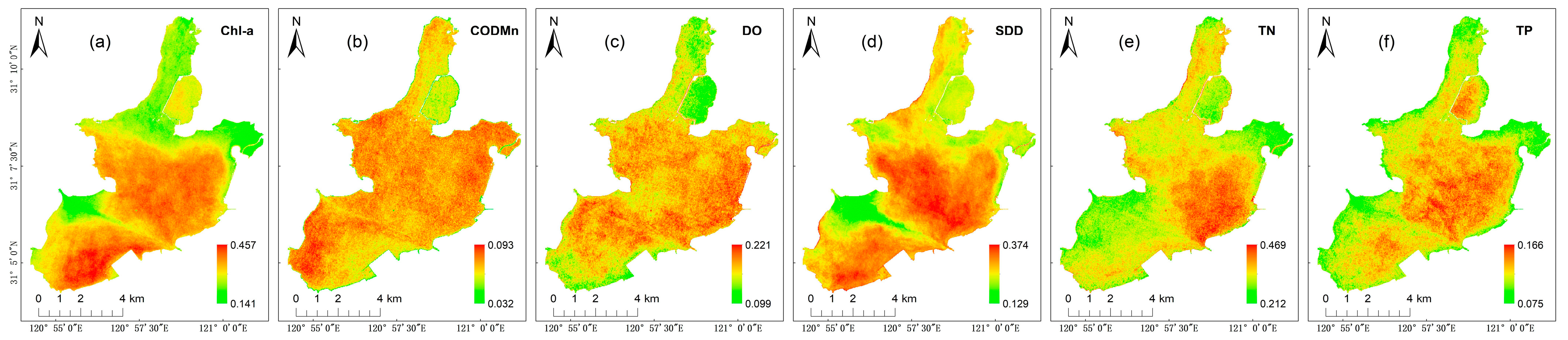
3.2.2. Spatial Variation
4. Discussion
4.1. Applicability of the Models
4.2. Performance and Evaluation of Machine Learning Algorithms
4.2.1. Analysis of Error Sources Affecting Model Performance
4.2.2. Evaluation of the Models
4.3. Spatiotemporal Change Analysis
4.4. Strengths and Limitations of the Study
5. Conclusions
Author Contributions
Funding
Data Availability Statement
Acknowledgments
Conflicts of Interest
Appendix A

| Water Quality Parameter | Determination Method |
|---|---|
| Chl-a | Nitrite Reduction Method and Continuous-Flow Analysis |
| CODMn | High-Temperature Oxidation Method and Continuous-Flow Analysis |
| DO | Electrode Method and Continuous-Flow Analysis |
| SDD | Potassium Permanganate Spectrophotometric Method and Continuous-Flow Analysis |
| TN | Ether Extraction–Spectrophotometric Method |
| TP | Transparency Meter Measurement |
| Model | Hyperparameters | Chl-a | CODMn | DO | SDD | TN | TP |
|---|---|---|---|---|---|---|---|
| RF | n_estimators | 450 | 500 | 360 | 390 | 490 | 300 |
| max_depth | 40 | 25 | 10 | 45 | 20 | 20 | |
| min_samples_split | 5 | 4 | 5 | 11 | 7 | 3 | |
| min_samples_leaf | 3 | 5 | 7 | 2 | 3 | 7 | |
| SVR | C | 4.91 | 2 | 8.67 | 9.82 | 7.52 | 2.94 |
| kernel | ‘rbf’ | ‘rbf’ | ‘rbf’ | ‘rbf’ | ‘rbf’ | ‘linear’ | |
| gamma | 88.109 | 58.907 | 29.329 | 80.078 | 66.251 | 16.369 | |
| XGBoost | learning_rate | 0.16 | 0.015 | 0.085 | 0.04 | 0.035 | 0.155 |
| gamma | 0.001 | 0.003 | 0.003 | 0.001 | 0.001 | 0.003 | |
| min_child_weight | 9 | 5 | 8 | 8 | 9 | 6 | |
| max_depth | 2 | 2 | 10 | 6 | 6 | 8 | |
| sub_sample | 1 | 1 | 0.8 | 1 | 0.8 | 1 | |
| reg_alpha | 0.1 | 1 | 1 | 0.01 | 1 | 0.01 | |
| CatBoost | iterations | 200 | 170 | 370 | 430 | 230 | 450 |
| learning_rate | 0.03 | 0.03 | 0.01 | 0.04 | 0.02 | 0.01 | |
| depth | 6 | 9 | 8 | 8 | 6 | 9 | |
| l2_leaf_reg | 2 | 1 | 2 | 9 | 2 | 2 |
References
- Ho, J.C.; Michalak, A.M.; Pahlevan, N. Widespread global increase in intense lake phytoplankton blooms since the 1980s. Nature 2019, 574, 667–670. [Google Scholar] [CrossRef]
- Yang, Z.; Gong, C.; Ji, T.; Hu, Y.; Li, L. Water Quality Retrieval from ZY1-02D Hyperspectral Imagery in Urban Water Bodies and Comparison with Sentinel-2. Remote Sens. 2022, 14, 5029. [Google Scholar] [CrossRef]
- Pi, X.; Feng, L.; Li, W.; Zhao, D.; Kuang, X.; Li, J. Water clarity changes in 64 large alpine lakes on the Tibetan Plateau and the potential responses to lake expansion. ISPRS-J. Photogramm. Remote Sens. 2020, 170, 192–204. [Google Scholar] [CrossRef]
- Ma, Y.; Song, K.; Wen, Z.; Liu, G.; Shang, Y.; Lyu, L.; Du, J.; Yang, Q.; Li, S.; Tao, H.; et al. Remote Sensing of Turbidity for Lakes in Northeast China Using Sentinel-2 Images with Machine Learning Algorithms. IEEE J. Sel. Top. Appl. Earth Observ. Remote Sens. 2021, 14, 9132–9146. [Google Scholar] [CrossRef]
- Cao, Z.; Ma, R.; Melack, J.M.; Duan, H.; Liu, M.; Kutser, T.; Xue, K.; Shen, M.; Qi, T.; Yuan, H. Landsat observations of chlorophyll-a variations in Lake Taihu from 1984 to 2019. Int. J. Appl. Earth Obs. Geoinf. 2022, 106, 102642. [Google Scholar] [CrossRef]
- Chen, J.; Lyu, Y.; Zhao, Z.; Liu, H.; Zhao, H.; Li, Z. Using the multidimensional synthesis methods with non-parameter test, multiple time scales analysis to assess water quality trend and its characteristics over the past 25 years in the Fuxian Lake, China. Sci. Total Environ. 2019, 655, 242–254. [Google Scholar] [CrossRef]
- Wang, J.; Fu, Z.; Qiao, H.; Liu, F. Assessment of eutrophication and water quality in the estuarine area of Lake Wuli, Lake Taihu, China. Sci. Total Environ. 2019, 650, 1392–1402. [Google Scholar] [CrossRef]
- Wang, Y.; Guo, Y.; Zhao, Y.; Wang, L.; Chen, Y.; Yang, L. Spatiotemporal heterogeneities and driving factors of water quality and trophic state of a typical urban shallow lake (Taihu, China). Environ. Sci. Pollut. Res. 2022, 29, 53831–53843. [Google Scholar] [CrossRef]
- Pahlevan, N.; Smith, B.; Alikas, K.; Anstee, J.; Barbosa, C.; Binding, C.; Bresciani, M.; Cremella, B.; Giardino, C.; Gurlin, D.; et al. Simultaneous retrieval of selected optical water quality indicators from Landsat-8, Sentinel-2, and Sentinel-3. Remote Sens. Environ. 2022, 270, 112860. [Google Scholar] [CrossRef]
- Shi, K.; Zhang, Y.; Zhu, G.; Qin, B.; Pan, D. Deteriorating water clarity in shallow waters: Evidence from long-term MODIS and in-situ observations. Int. J. Appl. Earth Obs. Geoinf. 2018, 68, 287–297. [Google Scholar] [CrossRef]
- Lee, Z.; Shang, S.; Hu, C.; Du, K.; Weidemann, A.; Hou, W.; Lin, J.; Lin, G. Secchi disk depth: A new theory and mechanistic model for underwater visibility. Remote Sens. Environ. 2015, 169, 139–149. [Google Scholar] [CrossRef]
- Sun, D.; Qiu, Z.; Li, Y.; Shi, K.; Gong, S. Detection of Total Phosphorus Concentrations of Turbid Inland Waters Using a Remote Sensing Method. Water Air Soil Pollut. 2014, 225, 1953. [Google Scholar] [CrossRef]
- Xu, W.; Duan, L.; Wen, X.; Li, H.; Li, D.; Zhang, Y.; Zhang, H. Effects of Seasonal Variation on Water Quality Parameters and Eutrophication in Lake Yangzong. Water 2022, 14, 2732. [Google Scholar] [CrossRef]
- Sagan, V.; Peterson, K.T.; Maimaitijiang, M.; Sidike, P.; Sloan, J.; Greeling, B.A.; Maalouf, S.; Adams, C. Monitoring inland water quality using remote sensing: Potential and limitations of spectral indices, bio-optical simulations, machine learning, and cloud computing. Earth-Sci. Rev. 2020, 205, 103187. [Google Scholar] [CrossRef]
- Chen, K.; Duan, L.; Liu, Q.; Zhang, Y.; Zhang, X.; Liu, F.; Zhang, H. Spatiotemporal Changes in Water Quality Parameters and the Eutrophication in Lake Erhai of Southwest China. Water 2022, 14, 3398. [Google Scholar] [CrossRef]
- Tian, S.; Guo, H.; Xu, W.; Zhu, X.; Wang, B.; Zeng, Q.; Mai, Y.; Huang, J.J. Remote sensing retrieval of inland water quality parameters using Sentinel-2 and multiple machine learning algorithms. Environ. Sci. Pollut. Res. 2023, 30, 18617–18630. [Google Scholar] [CrossRef] [PubMed]
- Duan, W.; Takara, K.; He, B.; Luo, P.; Nover, D.; Yamashiki, Y. Spatial, and temporal trends in estimates of nutrient and suspended sediment loads in the Ishikari River, Japan, 1985 to 2010. Sci. Total Environ. 2013, 461–462, 499–508. [Google Scholar] [CrossRef]
- Li, S.; Song, K.; Wang, S.; Liu, G.; Wen, Z.; Shang, Y.; Lyu, L.; Chen, F.; Xu, S.; Tao, H.; et al. Quantification of chlorophyll-a in typical lakes across China using Sentinel-2 MSI imagery with machine learning algorithm. Sci. Total Environ. 2021, 778, 146271. [Google Scholar] [CrossRef]
- Peterson, K.T.; Sagan, V.; Sloan, J.J. Deep learning-based water quality estimation and anomaly detection using Landsat-8/Sentinel-2 virtual constellation and cloud computing. GISci. Remote Sens. 2020, 57, 510–525. [Google Scholar] [CrossRef]
- Li, L.; Gu, M.; Gong, C.; Hu, Y.; Wang, X.; Yang, Z.; He, Z. An advanced remote sensing retrieval method for urban non-optically active water quality parameters: An example from Shanghai. Sci. Total Environ. 2023, 880, 163389. [Google Scholar] [CrossRef]
- Yang, H.; Kong, J.; Hu, H.; Du, Y.; Gao, M.; Chen, F. A Review of Remote Sensing for Water Quality Retrieval: Progress and Challenges. Remote Sens. 2022, 14, 1770. [Google Scholar] [CrossRef]
- Palmer, S.C.J.; Kutser, T.; Hunter, P.D. Remote sensing of inland waters: Challenges, progress and future directions. Remote Sens. Environ. 2015, 157, 1–8. [Google Scholar] [CrossRef]
- Topp, S.N.; Pavelsky, T.M.; Jensen, D.; Simard, M.; Ross, M.R.V. Research Trends in the Use of Remote Sensing for Inland Water Quality Science: Moving Towards Multidisciplinary Applications. Water. 2020, 12, 169. [Google Scholar] [CrossRef]
- Cao, Z.; Ma, R.; Duan, H.; Pahlevan, N.; Melack, J.; Shen, M.; Xue, K. A machine learning approach to estimate chlorophyll-a from Landsat-8 measurements in inland lakes. Remote Sens. Environ. 2020, 248, 111974. [Google Scholar] [CrossRef]
- Swain, R.; Sahoo, B. Improving river water quality monitoring using satellite data products and a genetic algorithm processing approach. Sustain. Water Qual. Ecol. 2017, 9–10, 88–114. [Google Scholar] [CrossRef]
- Xu, S.; Li, S.; Tao, Z.; Song, K.; Wen, Z.; Li, Y.; Chen, F. Remote Sensing of Chlorophyll-a in Xinkai Lake Using Machine Learning and GF-6 WFV Images. Remote Sens. 2022, 14, 5136. [Google Scholar] [CrossRef]
- Bramich, J.; Bolch, C.J.S.; Fischer, A. Improved red-edge chlorophyll-a detection for Sentinel 2. Ecol. Indic. 2021, 120, 106876. [Google Scholar] [CrossRef]
- Shi, X.; Gu, L.; Jiang, T.; Jiang, M.; Butler, J.J.; Xiong, X.J.; Gu, X. Retrieval of chlorophyll-a concentration based on Sentinel-2 images in inland lakes. In Proceedings of the Earth Observing Systems XXVII, San Diego, CA, USA, 23–25 August 2022; Volume 12232. [Google Scholar]
- Shi, X.; Gu, L.; Jiang, T.; Zheng, X.; Dong, W.; Tao, Z. Retrieval of Chlorophyll-a Concentrations Using Sentinel-2 MSI Imagery in Lake Chagan Based on Assessments with Machine Learning Models. Remote Sens. 2022, 14, 4924. [Google Scholar] [CrossRef]
- Yang, F.; He, B.; Zhou, Y.; Li, W.; Zhang, X.; Feng, Q. Trophic status observations for Honghu Lake in China from 2000 to 2021 using Landsat Satellites. Ecol. Indic. 2023, 146, 109898. [Google Scholar] [CrossRef]
- Gordon, H.R.; Clark, D.K.; Brown, J.W.; Brown, O.B.; Evans, R.H.; Broenkow, W.W. Phytoplankton pigment concentrations in the Middle Atlantic Bight: Comparison of ship determinations and CZCS estimates. Appl. Opt. 1983, 22, 20–36. [Google Scholar] [CrossRef]
- Schroeder, T.; Schaale, M.; Lovell, J.; Blondeau-Patissier, D. An ensemble neural network atmospheric correction for Sentinel-3 OLCI over coastal waters providing inherent model uncertainty estimation and sensor noise propagation. Remote Sens. Environ. 2022, 270, 112848. [Google Scholar] [CrossRef]
- Mouw, C.B.; Greb, S.; Aurin, D.; DiGiacomo, P.M.; Lee, Z.; Twardowski, M.; Binding, C.; Hu, C.; Ma, R.; Moore, T.; et al. Aquatic color radiometry remote sensing of coastal and inland waters: Challenges and recommendations for future satellite missions. Remote Sens. Environ. 2015, 160, 15–30. [Google Scholar] [CrossRef]
- Mobley, C.; Werdell, J.; Franz, B.A.; Ahmad, Z.; Bailey, S. Atmospheric Correction for Satellite Ocean Color Radiometry; NASA: Washington, DC, USA, 2016.
- Kuhn, C.; de Matos Valerio, A.; Ward, N.; Loken, L.; Sawakuchi, H.O.; Kampel, M.; Richey, J.; Stadler, P.; Crawford, J.; Striegl, R.; et al. Performance of Landsat-8 and Sentinel-2 surface reflectance products for river remote sensing retrievals of chlorophyll-a and turbidity. Remote Sens. Environ. 2019, 224, 104–118. [Google Scholar] [CrossRef]
- Niroumand-Jadidi, M.; Bovolo, F.; Bresciani, M.; Gege, P.; Giardino, C. Water Quality Retrieval from Landsat-9 (OLI-2) Imagery and Comparison to Sentinel-2. Remote Sens. 2022, 14, 4596. [Google Scholar] [CrossRef]
- He, Y.; Gong, Z.; Zheng, Y.; Zhang, Y. Inland Reservoir Water Quality Inversion and Eutrophication Evaluation Using BP Neural Network and Remote Sensing Imagery: A Case Study of Dashahe Reservoir. Water 2021, 13, 2844. [Google Scholar] [CrossRef]
- Shen, M.; Luo, J.; Cao, Z.; Xue, K.; Qi, T.; Ma, J.; Liu, D.; Song, K.; Feng, L.; Duan, H. Random forest: An optimal chlorophyll-a algorithm for optically complex inland water suffering atmospheric correction uncertainties. J. Hydrol. 2022, 615, 128685. [Google Scholar] [CrossRef]
- Ioannou, I.; Gilerson, A.; Gross, B.; Moshary, F.; Ahmed, S. Deriving ocean color products using neural networks. Remote Sens. Environ. 2013, 134, 78–91. [Google Scholar] [CrossRef]
- Chang, N.; Xuan, Z.; Yang, Y.J. Exploring spatiotemporal patterns of phosphorus concentrations in a coastal bay with MODIS images and machine learning models. Remote Sens. Environ. 2013, 134, 100–110. [Google Scholar] [CrossRef]
- Chang, N.; Vannah, B.W.; Yang, Y.J.; Elovitz, M. Integrated data fusion and mining techniques for monitoring total organic carbon concentrations in a lake. Int. J. Remote Sens. 2014, 35, 1064–1093. [Google Scholar] [CrossRef]
- Arias-Rodriguez, L.F.; Duan, Z.; Sepúlveda, R.; Martinez-Martinez, S.I.; Disse, M. Monitoring Water Quality of Valle de Bravo Reservoir, Mexico, Using Entire Lifespan of MERIS Data and Machine Learning Approaches. Remote Sens. 2020, 12, 1586. [Google Scholar] [CrossRef]
- Yuan, X.; Wang, S.; Fan, F.; Dong, Y.; Li, Y.; Lin, W.; Zhou, C. Spatiotemporal dynamics and anthropologically dominated drivers of chlorophyll-a, TN and TP concentrations in the Pearl River Estuary based on retrieval algorithm and random forest regression. Environ. Res. 2022, 215, 114380. [Google Scholar] [CrossRef] [PubMed]
- Xiong, G.; Wang, G.; Wang, D.; Yang, W.; Chen, Y.; Chen, Z. Spatio-Temporal Distribution of Total Nitrogen and Phosphorus in Dianshan Lake, China: The External Loading and Self-Purification Capability. Sustainability 2017, 9, 500. [Google Scholar] [CrossRef]
- Feng, L.; Hou, X.; Li, J.; Zheng, Y. Exploring the potential of Rayleigh-corrected reflectance in coastal and inland water applications: A simple aerosol correction method and its merits. ISPRS-J. Photogramm. Remote Sens. 2018, 146, 52–64. [Google Scholar] [CrossRef]
- Olmanson, L.G.; Brezonik, P.L.; Bauer, M.E. Evaluation of medium to low resolution satellite imagery for regional lake water quality assessments. Water Resour. Res. 2011, 47. [Google Scholar] [CrossRef]
- McFEETERS, S.K. The use of the Normalized Difference Water Index (NDWI) in the delineation of open water features. Int. J. Remote Sens. 1996, 17, 1425–1432. [Google Scholar] [CrossRef]
- Werther, M.; Odermatt, D.; Simis, S.G.H.; Gurlin, D.; Jorge, D.S.F.; Loisel, H.; Hunter, P.D.; Tyler, A.N.; Spyrakos, E. Characterising retrieval uncertainty of chlorophyll-a algorithms in oligotrophic and mesotrophic lakes and reservoirs. ISPRS-J. Photogramm. Remote Sens. 2022, 190, 279–300. [Google Scholar] [CrossRef]
- Wang, X.; Gong, C.; Ji, T.; Hu, Y.; Li, L. Inland water quality parameters retrieval based on the VIP-SPCA by hyperspectral remote sensing. J. Appl. Remote Sens. 2021, 15, 42609. [Google Scholar] [CrossRef]
- Lo, Y.; Fu, L.; Lu, T.; Huang, H.; Kong, L.; Xu, Y.; Zhang, C. Medium-Sized Lake Water Quality Parameters Retrieval Using Multispectral UAV Image and Machine Learning Algorithms: A Case Study of the Yuandang Lake, China. Drones 2023, 7, 244. [Google Scholar] [CrossRef]
- Guan, Q.; Feng, L.; Hou, X.; Schurgers, G.; Zheng, Y.; Tang, J. Eutrophication changes in fifty large lakes on the Yangtze Plain of China derived from MERIS and OLCI observations. Remote Sens. Environ. 2020, 246, 111890. [Google Scholar] [CrossRef]
- He, J.; Chen, Y.; Wu, J.; Stow, D.A.; Christakos, G. Space-time chlorophyll-a retrieval in optically complex waters that accounts for remote sensing and modeling uncertainties and improves remote estimation accuracy. Water Res. 2020, 171, 115403. [Google Scholar] [CrossRef]
- Mountrakis, G.; Im, J.; Ogole, C. Support vector machines in remote sensing: A review. ISPRS-J. Photogramm. Remote Sens. 2011, 66, 247–259. [Google Scholar] [CrossRef]
- Haghiabi, A.H.; Nasrolahi, A.H.; Parsaie, A. Water quality prediction using machine learning methods. Water Qual. Res. J. 2018, 53, 3–13. [Google Scholar] [CrossRef]
- Shenglei, W.; Junsheng, L.; Bing, Z.; Qian, S.; Fangfang, Z.; Zhaoyi, L. A simple correction method for the MODIS surface reflectance product over typical inland waters in China. Int. J. Remote Sens. 2016, 37, 6076–6096. [Google Scholar] [CrossRef]
- Zhang, Y.; Shi, K.; Cao, Z.; Lai, L.; Geng, J.; Yu, K.; Zhan, P.; Liu, Z. Effects of satellite temporal resolutions on the remote derivation of trends in phytoplankton blooms in inland waters. ISPRS-J. Photogramm. Remote Sens. 2022, 191, 188–202. [Google Scholar] [CrossRef]
- Li, J.; Gao, M.; Feng, L.; Zhao, H.; Shen, Q.; Zhang, F.; Wang, S.; Zhang, B. Estimation of Chlorophyll-a Concentrations in a Highly Turbid Eutrophic Lake Using a Classification-Based MODIS Land-Band Algorithm. IEEE J. Sel. Top. Appl. Earth Observ. Remote Sens. 2019, 12, 3769–3783. [Google Scholar] [CrossRef]
- Bentéjac, C.; Csörgő, A.; Martínez-Muñoz, G. A comparative analysis of gradient boosting algorithms. Artif. Intell. Rev. 2021, 54, 1937–1967. [Google Scholar] [CrossRef]
- Chen, Z.; An, C.; Tan, Q.; Tian, X.; Li, G.; Zhou, Y. Spatiotemporal analysis of land use pattern and stream water quality in southern Alberta, Canada. J. Contam. Hydrol. 2021, 242, 103852. [Google Scholar] [CrossRef] [PubMed]
- Huang, J.; Zhang, Y.; Bing, H.; Peng, J.; Dong, F.; Gao, J.; Arhonditsis, G.B. Characterizing the river water quality in China: Recent progress and on-going challenges. Water Res. 2021, 201, 117309. [Google Scholar] [CrossRef] [PubMed]
- Wang, S.; Ma, X.; Fan, Z.; Zhang, W.; Qian, X. Impact of nutrient losses from agricultural lands on nutrient stocks in Dianshan Lake in Shanghai, China. Water Sci. Eng. 2014, 7, 373–383. [Google Scholar]
| Water Quality Parameter | Range | Mean ± Std | Median | CV | N |
|---|---|---|---|---|---|
| Chl-a (mg/m3) | 1.34–51 | 15.04 ± 10.35 | 12.80 | 0.69 | 398 |
| CODMn (mg/L) | 2.10–7.00 | 3.96 ± 0.80 | 3.80 | 0.20 | 398 |
| DO (mg/L) | 3.90–13.84 | 8.73 ± 1.97 | 8.60 | 0.23 | 398 |
| TN (mg/L) | 0.33–5.23 | 2.04 ± 1.00 | 1.87 | 0.49 | 398 |
| TP (mg/L) | 0.03–0.26 | 0.10 ± 0.05 | 0.090 | 0.45 | 398 |
| SDD (m) | 0.1–1.1 | 0.42 ± 0.4 | 0.17 | 0.41 | 398 |
| Water Quality Parameter | Arrange | Mean ± Std | Median | CV | N |
|---|---|---|---|---|---|
| Chl-a (mg/m3) | 6.34–63.38 | 21.41–9.63 | 19.62 | 0.45 | 130 |
| CODMn (mg/L) | 3.37–5.15 | 4.24–0.42 | 4.30 | 0.10 | 130 |
| DO (mg/L) | 6.10–11.55 | 7.98–1.20 | 7.70 | 0.15 | 130 |
| TN (mg/L) | 0.24–0.53 | 0.36–0.07 | 0.34 | 0.19 | 130 |
| TP (mg/L) | 0.83–3.51 | 1.73–0.54 | 1.60 | 0.31 | 130 |
| SDD (m) | 0.066–0.329 | 0.112–0.029 | 0.111 | 0.26 | 130 |
| Band Combination Form | Chl-a | CODMn | DO | SDD | TN | TP |
|---|---|---|---|---|---|---|
| B7 1 B9 | B7 B2 | B6 B7 | B5 B2 | B2 B3 | B7 B6 | |
| B4 B5 | B6 B7 | B6 B7 | B2 B5 | B6 B7 | B7 B6 | |
| B4 B5 | B6 B7 | B6 B7 | B5 B2 | B7 B6 | B6 B7 | |
| B5 B4 B2 | B7 B6 B5 | B6 B7 B1 | B3 B5 B6 | B6 B7 B1 | B7 B6 B2 |
| Model | Hyperparameters | Options |
|---|---|---|
| RF | n_estimators | np.arange 1 (10, 600, 10) |
| max_depth | np.arange (10, 50, 5) | |
| min_samples_split | np.arange (1, 50, 1) | |
| min_samples_leaf | np.arange (1, 12, 1) | |
| SVR | C | np.arange (1, 10, 0.01) |
| kernel | [‘linear’, ‘rbf’,’sigmoid’] | |
| gamma | np.arange (1, 100, 0.001) | |
| XGBoost | learning_rate | np.arange (0.15, 0.2, 0.005) |
| gamma | np.arange (0.001, 0.005, 0.001) | |
| min_child_weight | np.arange (5, 10, 1) | |
| max_depth | np.arange (2, 10, 1) | |
| sub_sample | [0.8, 1] | |
| reg_alpha | [0.001, 0.01, 0.1, 1] | |
| CatBoost | iterations | np.arange (50, 500, 10) |
| learning_rate | np.arange (0.01, 0.05, 0.01) | |
| depth | np.arange (2,10,1) | |
| l2_leaf_reg | np.arange (1,10,1) |
| Water Quality Parameter | RMSE | MAPE | Bias |
|---|---|---|---|
| Chl-a | 19.88 mg/m3 | 44.88% | −12.14 mg/m3 |
| CODMn | 0.74 mg/L | 14.61% | 0.08 mg/L |
| DO | 1.69 mg/L | 14.88% | −1.25 mg/L |
| SDD | 0.07 m | 15.7% | −0.013 m |
| TN | 1.5 mg/L | 54.78% | 10.45 mg/L |
| TP | 0.05 mg/L | 67.56% | 0.034 mg/L |
| Parameters | Methods | 1 × 1 | 3 × 3 | 5 × 5 | |||
|---|---|---|---|---|---|---|---|
| RMSE | MAPE (%) | RMSE | MAPE (%) | RMSE | MAPE (%) | ||
| Chl-a (mg/m3) | CatBoost | 11.19 | 29.12 | 11.11 | 28.12 | 11.21 | 29.12 |
| RF | 10.94 | 29.87 | 10.94 | 29.57 | 10.99 | 31.57 | |
| SVR | 13.99 | 38.15 | 12.99 | 35.15 | 13.99 | 39.15 | |
| XGBoost | 10.46 | 29.86 | 10.46 | 30.86 | 10.96 | 31.86 | |
| CODMn (mg/L) | CatBoost | 0.58 | 11.29 | 0.57 | 11.24 | 0.59 | 11.87 |
| RF | 0.60 | 11.33 | 0.58 | 11.28 | 0.62 | 12.19 | |
| SVR | 0.61 | 11.63 | 0.60 | 11.10 | 0.61 | 12.11 | |
| XGBoost | 0.57 | 10.60 | 0.55 | 10.55 | 0.57 | 11.32 | |
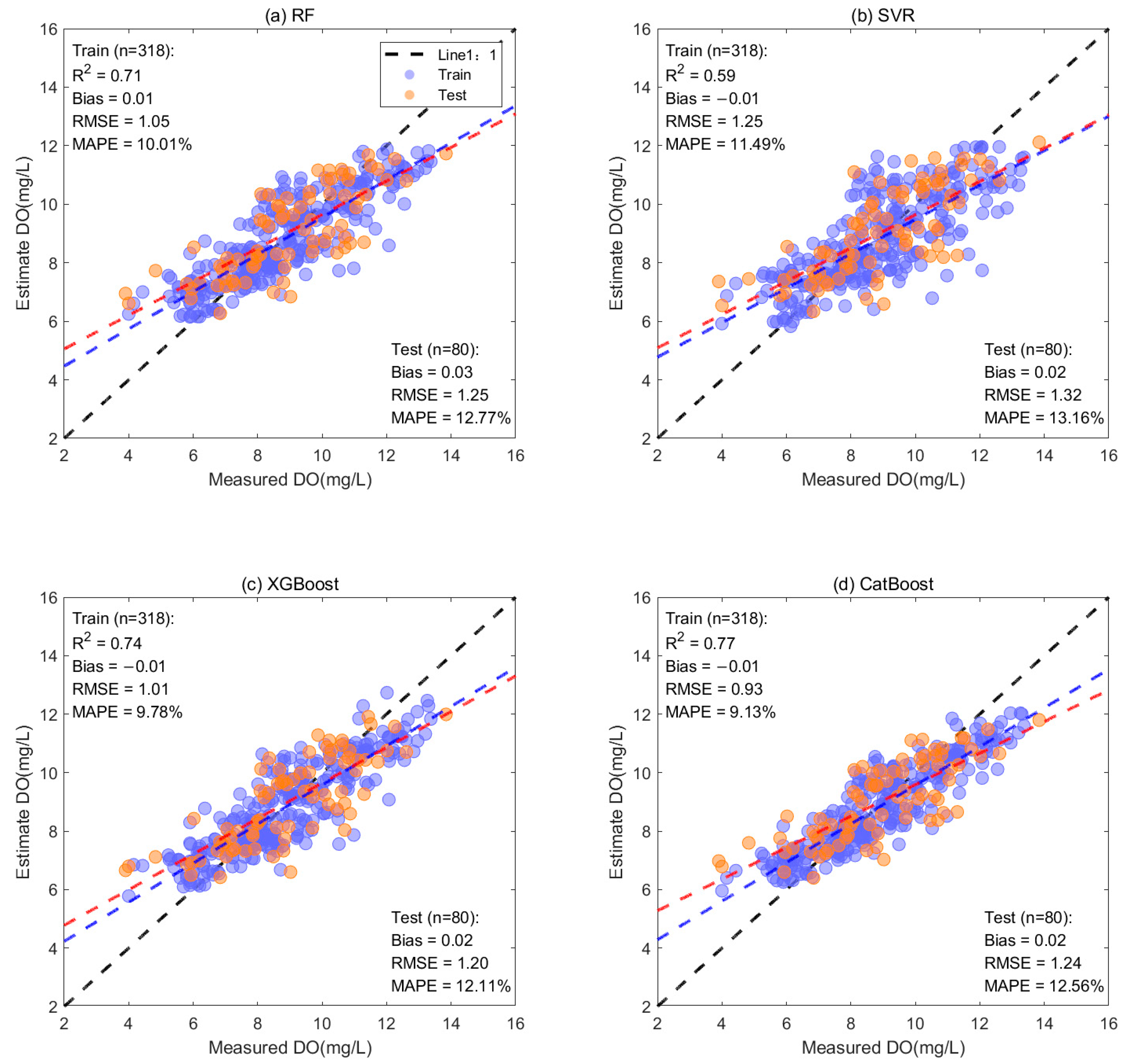
| DO (mg/L) | CatBoost | 1.27 | 12.89 | 1.25 | 12.77 | 1.31 | 13.16 |
| RF | 1.32 | 13.24 | 1.32 | 13.16 | 1.35 | 13.68 | |
| SVR | 1.24 | 12.29 | 1.20 | 12.11 | 1.24 | 12.29 | |
| XGBoost | 1.34 | 13.14 | 1.24 | 12.56 | 1.28 | 12.97 | |
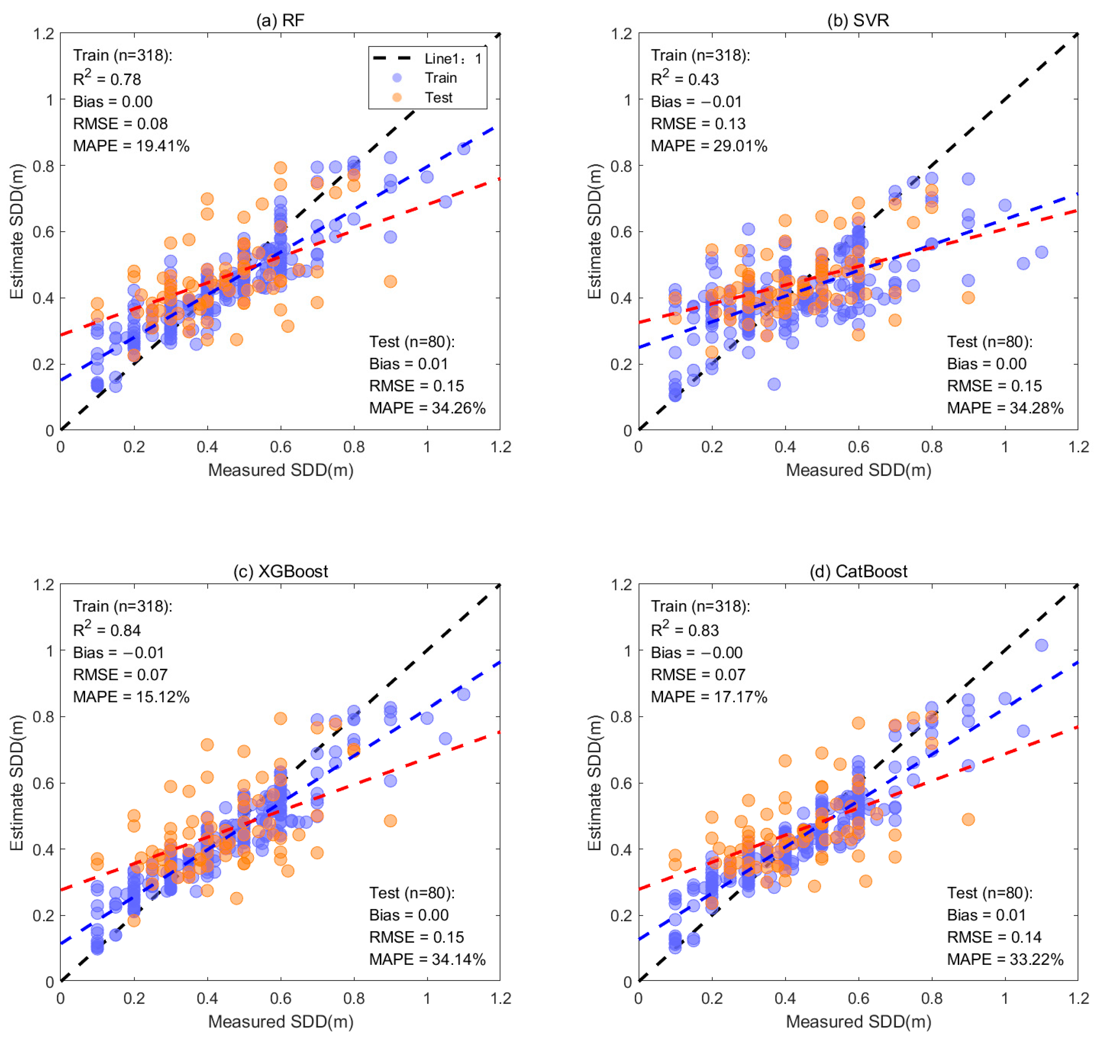
| SDD (m) | CatBoost | 14.44 | 34.38 | 14.73 | 34.26 | 14.65 | 34.63 |
| RF | 14.69 | 34.44 | 14.77 | 34.28 | 14.75 | 34.90 | |
| SVR | 14.80 | 34.14 | 14.74 | 34.14 | 14.81 | 34.57 | |
| XGBoost | 14.38 | 34.03 | 14.15 | 33.22 | 14.35 | 34.31 | |
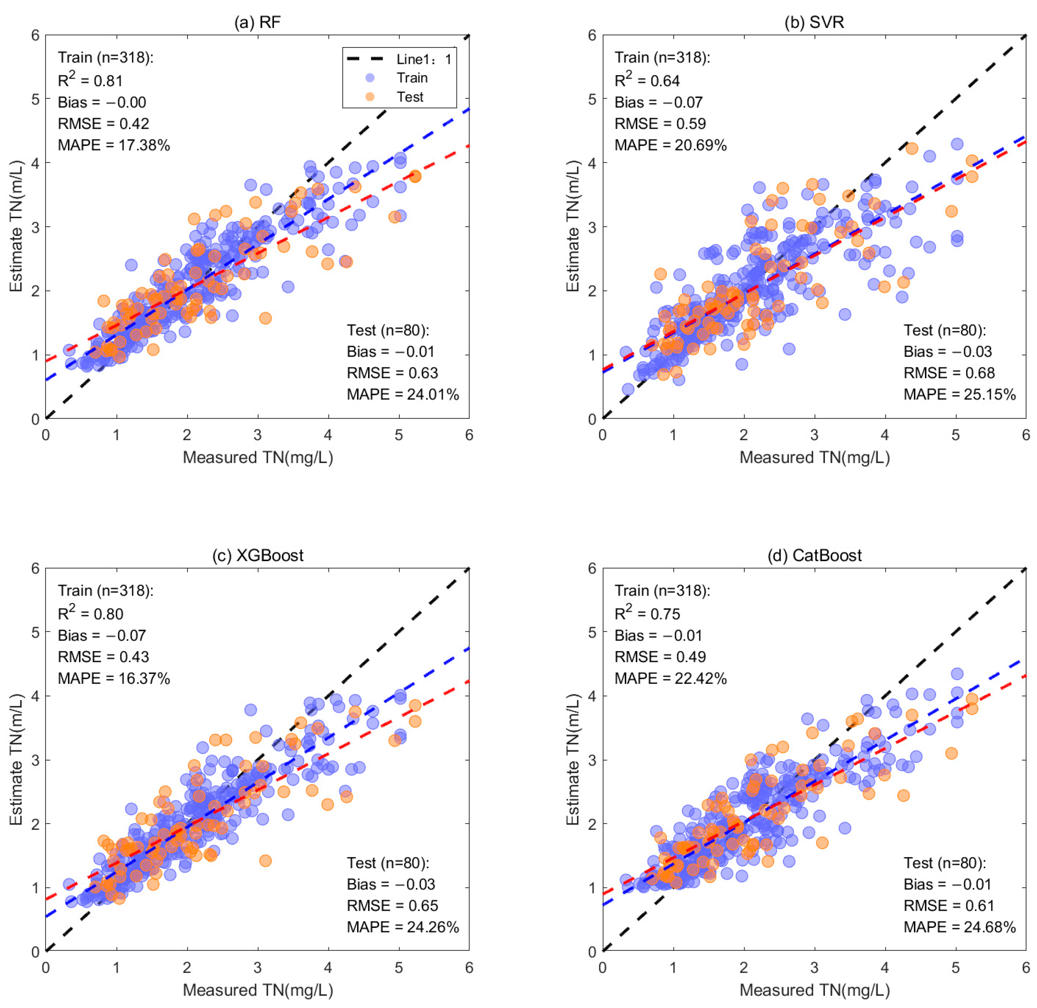
| TN (mg/L) | CatBoost | 0.72 | 25.83 | 0.63 | 24.01 | 0.68 | 26.14 |
| RF | 0.82 | 26.08 | 0.68 | 25.15 | 0.65 | 26.33 | |
| SVR | 0.73 | 24.80 | 0.65 | 24.26 | 0.62 | 25.07 | |
| XGBoost | 0.69 | 25.81 | 0.61 | 24.68 | 0.61 | 24.76 | |
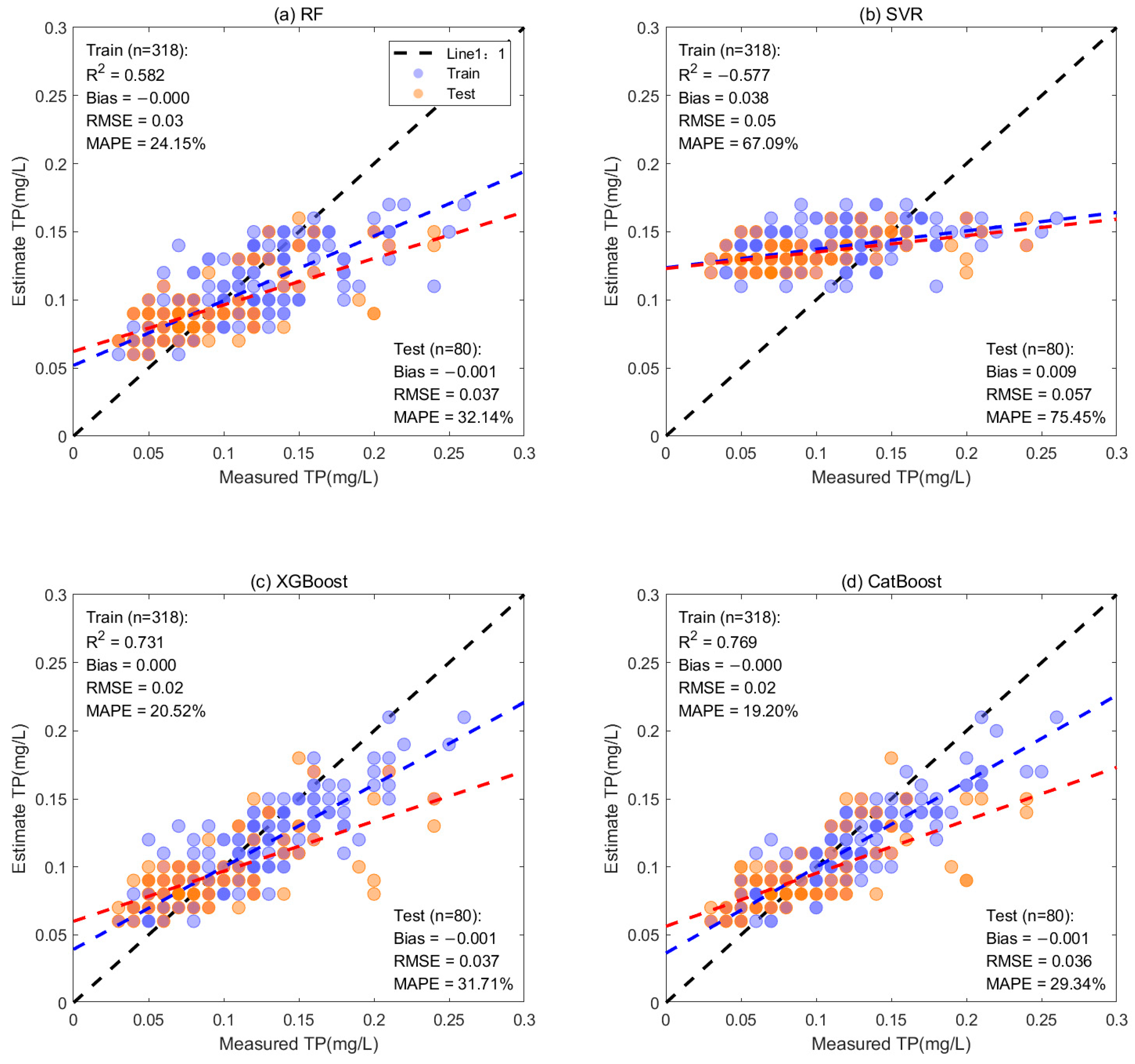
| TP (mg/L) | CatBoost | 0.04 | 33.13 | 0.04 | 32.14 | 0.04 | 32.91 |
| RF | 0.06 | 78.09 | 0.06 | 75.45 | 0.06 | 74.07 | |
| SVR | 0.04 | 32.47 | 0.04 | 31.71 | 0.04 | 32.02 | |
| XGBoost | 0.04 | 30.20 | 0.04 | 29.34 | 0.04 | 31.88 | |
| Index | Chl-a | CODMn | DO | SDD | TN | TP |
|---|---|---|---|---|---|---|
| Water temperature | 0.38 | 0.71 * | −0.94 * | −0.86 * | −0.32 | −0.1 |
| PH | 0.73 * | 0.46 | −0.35 | −0.19 | −0.24 | −0.25 |
| Conductivity | −0.4 | −0.12 | 0.43 | 0.56 | 0.38 | 0.39 |
| Air temperature | 0.41 | 0.82 * | −0.97 * | −0.82 * | −0.35 | −0.13 |
| Precipitation | 0.78 * | 0.45 | −0.72 * | −0.42 | −0.67 * | −0.37 |
| Wind speed | 0.15 | 0.43 | −0.42 | −0.21 | −0.49 | −0.33 |
Disclaimer/Publisher’s Note: The statements, opinions and data contained in all publications are solely those of the individual author(s) and contributor(s) and not of MDPI and/or the editor(s). MDPI and/or the editor(s) disclaim responsibility for any injury to people or property resulting from any ideas, methods, instructions or products referred to in the content. |
© 2023 by the authors. Licensee MDPI, Basel, Switzerland. This article is an open access article distributed under the terms and conditions of the Creative Commons Attribution (CC BY) license (https://creativecommons.org/licenses/by/4.0/).
Share and Cite
Dong, L.; Gong, C.; Huai, H.; Wu, E.; Lu, Z.; Hu, Y.; Li, L.; Yang, Z. Retrieval of Water Quality Parameters in Dianshan Lake Based on Sentinel-2 MSI Imagery and Machine Learning: Algorithm Evaluation and Spatiotemporal Change Research. Remote Sens. 2023, 15, 5001. https://doi.org/10.3390/rs15205001
Dong L, Gong C, Huai H, Wu E, Lu Z, Hu Y, Li L, Yang Z. Retrieval of Water Quality Parameters in Dianshan Lake Based on Sentinel-2 MSI Imagery and Machine Learning: Algorithm Evaluation and Spatiotemporal Change Research. Remote Sensing. 2023; 15(20):5001. https://doi.org/10.3390/rs15205001
Chicago/Turabian StyleDong, Lei, Cailan Gong, Hongyan Huai, Enuo Wu, Zhihua Lu, Yong Hu, Lan Li, and Zhe Yang. 2023. "Retrieval of Water Quality Parameters in Dianshan Lake Based on Sentinel-2 MSI Imagery and Machine Learning: Algorithm Evaluation and Spatiotemporal Change Research" Remote Sensing 15, no. 20: 5001. https://doi.org/10.3390/rs15205001
APA StyleDong, L., Gong, C., Huai, H., Wu, E., Lu, Z., Hu, Y., Li, L., & Yang, Z. (2023). Retrieval of Water Quality Parameters in Dianshan Lake Based on Sentinel-2 MSI Imagery and Machine Learning: Algorithm Evaluation and Spatiotemporal Change Research. Remote Sensing, 15(20), 5001. https://doi.org/10.3390/rs15205001