Mapping Underwater Aquatic Vegetation Using Foundation Models With Air- and Space-Borne Images: The Case of Polyphytos Lake

Abstract

Mapping underwater aquatic vegetation (UVeg) is crucial for understanding the dynamics of freshwater ecosystems. The advancement of artificial intelligence (AI) techniques has shown great potential in improving the accuracy and efficiency of UVeg mapping using remote sensing data. This paper presents a comparative study of the performance of classical and modern AI tools, including logistic regression, random forest, and a visual-prompt-tuned foundational model, the Segment Anything model (SAM), for mapping UVeg by analyzing air- and space-borne images in the few-shot learning regime, i.e., using limited annotations. The findings demonstrate the effectiveness of the SAM foundation model in air-borne imagery ($GSD$ = 3–6 cm) with an $F1$ score of $86.5\%\pm 4.1\%$ when trained with as few as 40 positive/negative pairs of pixels, compared to $54.0\%\pm 9.2\%$ using the random forest model and $42.8\%\pm 6.2\%$ using logistic regression models. However, adapting SAM to space-borne images (WorldView-2 and Sentinel-2) remains challenging, and could not outperform classical pixel-wise random forest and logistic regression methods in our task. The findings presented provide valuable insights into the strengths and limitations of AI models for UVeg mapping, aiding researchers and practitioners in selecting the most suitable tools for their specific applications.

1. Introduction

Aquatic vegetation holds immense significance within ecosystems, as it not only supports the food chain but also serves as the primary indicator of ecosystem quality [1]. Detailed information on the distribution, composition, and abundance of aquatic vegetation is widely utilized to assess the environmental quality of aquatic systems, thereby playing a crucial role in maintaining the proper functioning of lakes. In particular, submerged, or in general, underwater aquatic vegetation (UVeg), comprising plants that primarily grow underwater but may possess floating or emerged reproductive organs, plays a vital ecological and environmental role. These plants fulfill crucial functions, including providing habitat for various species, stabilizing sediments, regulating water flow, acting as a natural purifier, and participating in the biogeochemical cycling process [2].

Precise identification of UVeg distribution and growth duration can provide valuable information for effective lake management and future ecological restoration endeavors. As a result, numerous national and international water quality frameworks, including those employed by the European Union, integrate the assessment of submerged aquatic vegetation extent or health as key indicators in their evaluations. Remote sensing technology, particularly satellite data, has emerged as an effective tool for mapping UVeg. In particular, multi-spectral data have been extensively employed for mapping the distribution of large-scale aquatic vegetation and evaluating its intra-annual and inter-annual variations [3,4,5,6].

However, accurately distinguishing between submerged aquatic vegetation and emergent or floating vegetation remains a complex task through satellite data. The transitional nature of aquatic vegetation, influenced by factors such as incomplete development, seasonality, water level fluctuations, and flooding events, poses significant challenges for accurate classification using remote sensing techniques. In light of these complexities, our research aims to overcome these limitations by focusing on monitoring all forms of vegetation occurring beneath the water surface. While our previous work [7] focused solely on identifying emergent and floating aquatic vegetation, our attention in this study lies on underwater aquatic vegetation, which encompasses all forms of vegetation occurring in submerged or partially submerged conditions.

To provide a comprehensive overview of the existing techniques, Rowan and Kalacska [2] conducted a review specifically tailored for non-specialists. Their paper discusses the challenges associated with UVeg mapping using remote sensing, such as water attenuation, spectral complexity, and spatial heterogeneity. Furthermore, they provide an overview of different remote sensing platforms, including aerial and space-borne sensors, commonly used for UVeg mapping and argue that understanding the capabilities and limitations of these platforms is crucial in selecting the appropriate tools for UVeg mapping. The authors also discuss the specific spectral characteristics of UVeg, as well as classification methods, and finally, they highlight the importance of validation and accuracy assessment in UVeg mapping studies. By incorporating insights from this review, our study aims to contribute to the existing knowledge and further enhance the accuracy and efficiency of UVeg mapping using remote sensing data.

The study of Villa et al. [8] introduces a rule-based approach for mapping macrophyte communities using multi-temporal aquatic vegetation indices. Their study emphasizes the importance of considering temporal variations in vegetation indices and proposes a classification scheme based on rules derived from these indices. The approach shows promising results in accurately mapping macrophyte communities, providing valuable insights for ecological assessments and environmental monitoring. The paper by Husson et al. [9] highlights the use of unmanned aircraft vehicles (UAVs) for mapping aquatic vegetation. They discuss the advantages of UAVs, such as high spatial resolution and cost-effectiveness. Their study demonstrates the accuracy of UAV-based vegetation mapping, including species distribution and habitat heterogeneity. UAV imagery provides detailed information for ecological research and conservation efforts. The paper also addresses challenges and suggests future directions for optimizing UAV-based methods in aquatic vegetation mapping. Heege et al. [10] presented the Modular Inversion Program (MIP), a processing tool that utilizes remote sensing data to map submerged vegetation in optically shallow waters. MIP incorporates modules for calculating the bottom reflectance and fractionating it into specific reflectance spectra, enabling mapping of different types of vegetation.

Machine learning (ML) approaches in remote sensing offer efficient and accurate methods for analyzing vast amounts of satellite data and extracting valuable insights about the Earth’s surface and environment. However, previous studies on classifying wetland vegetation have often focused on single sites and lacked rigorous testing of the generalization capabilities. To fill this gap, Piaser et al. [11] compiled an extensive reference dataset of about 400,000 samples covering nine different sites and multiple seasons to represent temperate wetland vegetation communities at a continental scale. They compared the performance of eight ML classifiers, including support vector machine (SVM), random forest (RF), and XGBoost, using multi-temporal Sentinel-2 data as input features. According to their findings, the top choices for mapping macrophyte community types in temperate areas, as explored in this study, are SVM, RF, and XGBoost. Reducing the number of input features led to accuracy degradation, emphasizing the effectiveness of multi-temporal spectral indices for aquatic vegetation mapping.

The debate between classical ML techniques and deep learning (DL) revolves around computational resources and the available annotated datasets. Classical ML can achieve high discriminative performance with moderate processing speed, making it suitable for scenarios with limited computational resources [12]. In contrast, DL’s undeniable success in computer vision tasks, particularly in remote sensing imagery [13,14], comes at the expense of requiring substantial computational resources. Additionally, DL models are data-hungry during training, posing challenges for the few-shot learning tasks commonly encountered in remote sensing applications. Despite this, techniques like pre-training on other datasets, data augmentation, and, most importantly, self-supervised learning (SSL) exist to mitigate this issue.

Based on SSL, foundation models came recently to the forefront of machine learning research, offering a unified, versatile approach that learns across various tasks and domains. As illustrated by Bommasani et al. [15], a key advantage of foundation models lies in their ability to perform with limited annotations, utilizing pre-existing knowledge to make sense of sparse or partially labeled data. The Segment Anything model (SAM) [16] epitomizes this advantage with its ability to effectively segment any class in an image, making it especially suitable for the analysis of complex and often poorly annotated environments.

In this study, we harness the capabilities of SAM in mapping and analyzing the underwater aquatic vegetation in Polyphytos Lake, Greece. Our approach combines a range of remote sensing data, including multi-spectral satellite images from WorldView-2 and Sentinel-2, UAV-acquired data, and expert annotations from marine biologists, in collaboration with local water service authorities.

Given the often-scarce annotations in aquatic ecosystem studies, the application of foundation models, such as SAM, offers a powerful tool to gain insights into aquatic vegetation, water quality, and potential pollution sources. The subsequent sections of this paper will detail our methodology, challenges, results, and their implications, demonstrating the significant potential of foundation models in data-scarce, complex environments like aquatic ecosystems.

2. Materials and Methods

2.1. Study Area

Our study took place at the Polyphytos reservoir, as shown in Figure 1 an artificial lake on the Aliakmon River, located in West Macedonia, Northern Greece, specifically in Kozani province. The reservoir’s surface area is $75{\mathrm{km}}^2$. The reservoir was formed in 1975 when a dam was built on the Aliakmon River close to the Polyphytos village. The longest dimension of the lake is 31 km and the widest is $2.5$ km. It is the biggest of five reservoirs built along the river, with a drainage area of 5630 square kilometers, and it collects water from surface runoff and several torrents.

The reservoir is used to produce hydroelectric power and supply irrigation water, and since 2003, it has been the main source of drinking water for Thessaloniki, the second-largest city in Greece, with a population of 1.05 million people. Every day, around 145,000 cubic meters of surface water is taken from the Polyphytos Reservoir to Thessaloniki’s Drinking Water Treatment Plant (TDWTP).

The Polyphytos region has a continental climate with cold winters and mild summers. The region’s rainfall is not very high, but previous studies [17] have shown that rainfall does not drop much during summer. However, the months from June to September are seen as dry because of the relatively low average rainfall.

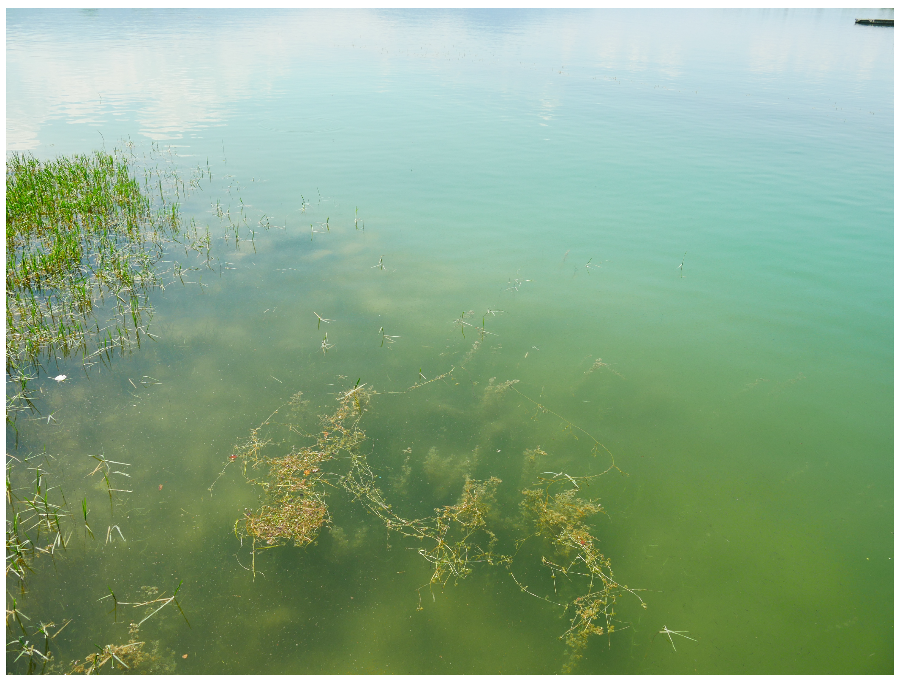
Over the years, Polyphytos Lake has transformed into a significant sanctuary for birds and a thriving environment for many fish species. Regarding vegetation, the vicinity of the reservoir boasts a considerable expanse of wetlands, marshlands, and muddy ecosystems. Additionally, a range of aquatic plant life resides within the Polyphytos Reservoir, e.g., as show in Figure 2, contributing to the area’s rich ecological diversity.

2.2. Data Sources

We obtained multi-spectral satellite images from two sources: WorldView-2 and Sentinel-2. The WorldView-2 images provided high-resolution data with a ground sampling distance (GSD) of 1.8 m, enabling detailed observation of the lake and its surrounding areas. The Sentinel-2 images complemented the WorldView-2 data by offering additional spectral information for our analysis, although with the lowest GSD of 10 m. In order to acquire more granular and comprehensive data, we executed a UAV survey over Polyphytos Lake. We deployed the DJI Mini 3 Pro UAV, maintaining a flight altitude between 50 and 70 m. The UAV came equipped with a high-resolution camera, enabling us to gather detailed and current data on the lake’s attributes. A description of the data sources used in the study is given in

Table 1. Summary of data sources, specifications, and sensing dates.

Data Source	Area	GSD	Dates
WorldView-2	AOI 1	1.8 m	31 August 2020
Sentinel-2	AOI 1	10–60 m	16, 21, 26 and 31 August 2020 5, 10 and 15 September 2020
DJI Mini 3 Pro UAV	AOI 1–3	3–6 cm	6 March 2023

.

2.3. Dataset Annotation

Through information exchange with local water service authorities and in situ visits by the authors, detailed annotations could be retrieved, specifically focusing on the UVeg present in Polyphytos Lake. The meticulous identification and labeling of underwater vegetation formations at various scales and depths using multiple uncertainty classes ensure the accuracy and reliability of these annotations. The availability of such comprehensive annotations allows us to assess the performance and effectiveness of our AI tools in accurately mapping and monitoring UVeg in Polyphytos Lake, providing valuable insights into the distribution, health, and ecological significance of underwater vegetation in the lake.

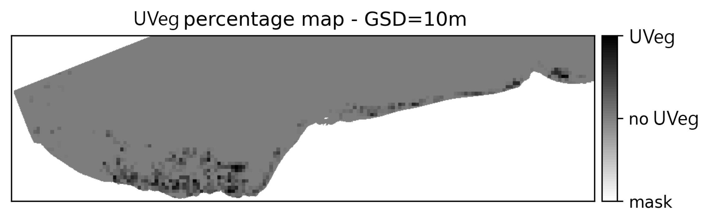
Manual annotation was performed separately for the WorldView-2 and UAV imagery, while the annotations of the Sentinel-2 data were extracted based on the WorldView-2 annotations. Due to the proximity of dates, we assume no modification in vegetation extent (UVeg extent). Therefore, only adaptation of the spatial resolution was performed by transforming the binary values of the pixels in the lower ground sampling distance (GSD) of WorldView-2 to percentage values of the higher-GSD pixels of Sentinel-2m, as shown in Figure 3.

2.4. Comparison of ML Techniques

In this work, we compare two different AI methodologies for segmenting UVeg in Polyphytos Lake:

• Pixel-based Logistic Regression or Random Forest:

The first approach utilizes classical machine learning techniques such as logistic regression and random forest. In this method, we extract various spectral and textural features from the multi-spectral satellite images and UAV data. These features are then used to train pixel-based classification models, which can classify each pixel as either UVeg or non-UVeg. Logistic regression and random forest algorithms are employed for the classification task, leveraging their ability to learn complex relationships between the input features and the UVeg class labels. We recognize random forest, which is a bagging model, together with boosting models as powerful and widely-used ML techniques based on ensembling [11,12]. Additionally, we included logistic regression as a baseline ML method, as it represents traditional thresholding techniques commonly found in remote sensing studies when combining linear combinations of bands.

Apart from the multi-spectral bands, we utilized the QAA-RGB algorithm [18], a modified version of the quasi-analytical algorithm (QAA), to detect underwater vegetation in Polyphytos Lake using only the red, green, and blue bands. The algorithm was specifically designed for high-resolution satellite sensors, and it retrieves various parameters, including the total absorption, particle backscattering, diffuse attenuation coefficient, and Secchi disk depth, which have been used as additional features in our comparative analysis. By using remote sensing reflectance data from three specific bands (red, green, and blue), the algorithm ensures robustness and applicability across different water types. The implementation of QAA-RGB was carried out within the ACOLITE processor, which provides a comprehensive and accessible platform for the scientific community.

• Foundation Model for Semantic Segmentation with Prompt-tuning:

The second approach utilizes a foundation model called SAM (Segment Anything) [16]. SAM is a state-of-the-art deep learning model designed specifically for semantic segmentation tasks. It is pretrained on a large-scale dataset, enabling it to learn general patterns and features related to segmentation. However, what sets SAM apart is its prompt-tuning approach. During fine-tuning, SAM is provided with a small set of positive and negative UVeg pixels as prompts. These prompts guide the model to learn the specific characteristics and boundaries of UVeg in Polyphytos Lake. By adaptively adjusting the prompts, SAM refines its segmentation capabilities and improves its accuracy in detecting and delineating UVeg regions.

In our model evaluation, we employed three key metrics computed from the number of pixels as true positive ($TP$), true negative ($TN$), false positive ($FP$), and false negative ($FN$):

$PA$, the producer’s accuracy (recall), quantifies the percentage of correctly classified pixels in relation to the ground truth, thus representing the model’s ability to accurately identify and classify true positive instances:

$$PA=\frac{TP}{TP+FN}$$

$UA$, the user’s accuracy (precision), measures the percentage of correctly classified pixels based on the model’s predictions, reflecting the precision of the model in accurately identifying and classifying true positive instances:

$$UA=\frac{TP}{TP+FP}$$

Additionally, we computed the $F1$ score, a commonly used metric for evaluating such models. The $F1$ score can be interpreted as a weighted average of the precision ($UA$) and recall ($PA$), where an $F1$ score reaches its best value at 1 (perfect precision and recall) and worst at 0. It is defined as:

$$F1=2\ast \frac{UA\ast PA}{UA+PA}$$

The $F1$ score tries to balance these two measures. A good $F1$ score indicates low false positives and low false negatives, which are especially important when false positives and false negatives have different costs, often the case in imbalanced datasets.

We established baselines for all three modalities—UAV RGB images, multi-spectral images from WorldView-2, and Sentinel-2 sensors—using logistic regression. To mitigate the effects of the imbalanced dataset in all three modalities, we employed resampling methods during the training phase. These involve artificially augmenting the dataset by repeating uniformly selected samples to ensure an equal representation of samples from different classes. This approach not only enhances the performance of logistic regression, but also provides an unbiased analysis for feature importance [19].

We further conducted a comparative analysis of three data sources using k-fold cross-validation. To account for the significant differences in dataset size among the modalities, we utilized different numbers of folds for each modality. This approach ensured that the training sets were sufficiently large for modalities with a smaller total number of pixels. To evaluate the performance of our models, we computed metrics based on the concatenated confusion matrices obtained from each fold. Instead of calculating the average values of metrics separately for each fold, this approach provides a more robust assessment. Specifically, for the Sentinel-2 modality, where the number of available pixels from the positive class is limited, averaging the metrics across folds can introduce bias into the estimate [20]. For the SAM method, resampling with replacement of a fixed number of pixel pairs was performed with 500 repetitions.

In addition, we carried out ablation studies on single-, double-, and triple-feature classifiers. The objective was to investigate the influence of feature selection on the predictive accuracy of our per-pixel classification model. By systematically excluding features from the model, we were able to quantify the contribution of each individual feature or combination of features. The evaluation of these ablation studies was based on the $F1$ metric. Through this ablation study, we obtained valuable insights into how different bands, or their combinations, affect the accuracy of the model in classifying UVeg pixels. This, consequently, directed our optimization of the band-selection process to apply the SAM, a foundation model that utilizes only three bands. A more sophisticated feature-importance analysis of WorldView-2 data was performed, focusing on pixel proximity to the shore. Specifically, apart from the analysis in the total WorldView-2 image, the analysis was also conducted on a manually selected subset of the image near the shore with a higher density of visually apparent UVeg regions, referred to as “shallow pixels”. The areas of the lake farther from the shore did not exhibit visually apparent UVeg, likely due to the lake’s depth.

Moreover, we conducted an extensive analysis of the two SAM variants, “huge” and “base”, utilizing the ViT-B and ViT-H encoders developed by Meta AI Research and FAIR (https://github.com/facebookresearch/segment-anything, accessed on 10 July 2023). SAM has two encoder options: ViT-B (91M parameters) and ViT-H (636M parameters). The primary objective of this analysis is to gain insights into the performance disparities between the two variants under the few-shot learning task of segmenting UVeg.

In the context of the Sentinel-2 data source, we investigated the use of multi-class classification by comparing the performance of models with 2–4 classes instead of using a regression-based approach. Here, the number of classes refers to distinct categories or groups into which the satellite data can be classified. In a 2-class model, the data would be divided into two distinct categories, which might correspond to the “presence” or “absence” of a certain feature in the satellite imagery, for example. For the 3-class model, the data would be divided into three categories, possibly representing low, medium, and high levels of a certain feature. In the 4-class model, there would be four different categories, potentially providing an even finer granularity of the measured feature. Since the task was not binary classification but multi-class, we used the metric of balanced accuracy to evaluate the performance. Balanced accuracy is the average of the recall (the proportion of actual positives that are correctly identified) obtained for each class, which ensures that every class is equally weighted regardless of how often it appears in the data. This was particularly relevant because of the multi-class nature of our models. By comparing the 2-, 3-, and 4-class models, we were able to rigorously evaluate how different levels of class granularity impacted the accuracy of our Sentinel-2 data classifications.

Finally, to assess the transferability of the models in different areas of interest (AOIs) within the lake, a logistic regression model and a random forest model were trained on AOI1 near the Rymnio bridge and evaluated on AOI2 and AOI3 (described in Table 1). The random forest model underwent hyperparameter tuning using a validation set from AOI1, while testing was conducted separately on the different lake AOIs [21].

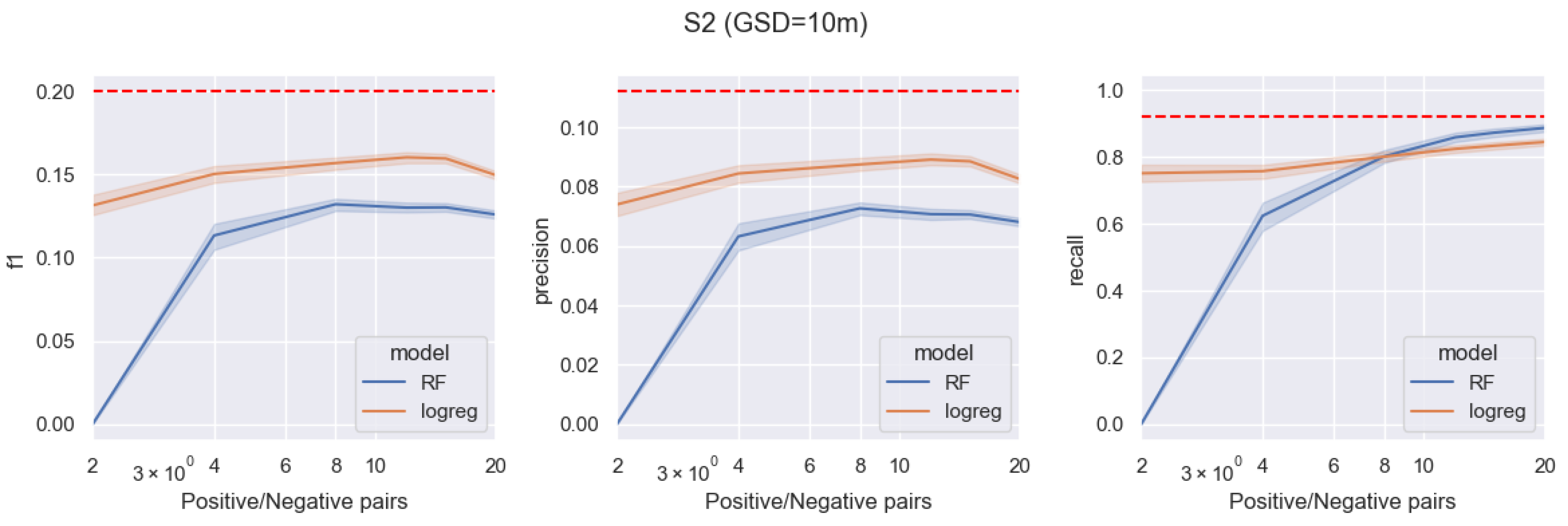
3. Results

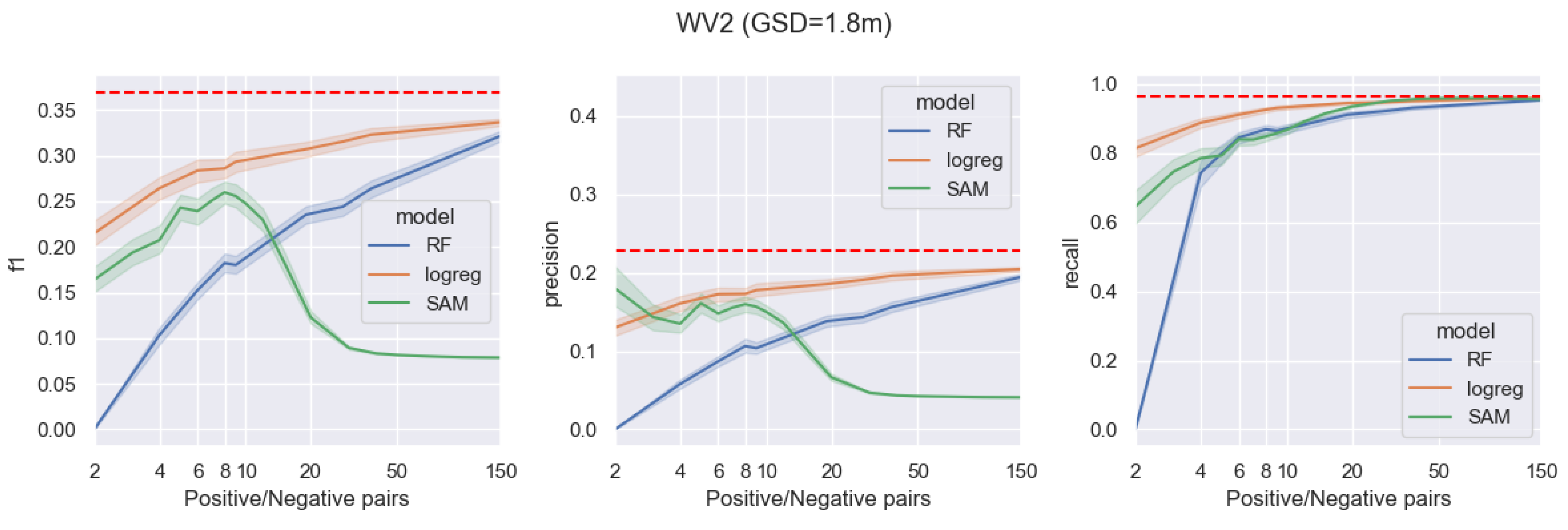
The primary findings from the comparative study on segmenting underwater aquatic vegetation data based on very limited annotations are illustrated in Figure 4, Figure 5 and Figure 6. This study provides an exhaustive comparison of three machine learning techniques, namely a logistic regression model, a random forest model, and a foundational model referred to as the Segment Anything Model (SAM). The SAM model, which is based on the Vision Transformer architecture, is pretrained for the task of semantic segmentation and is specifically tailored for visual prompting. The comparative analysis is carried out across three distinct data sources: UAV, WorldView-2, and Sentinel-2. Baseline measures for each metric, represented as red dashed lines, are computed based on the training error of the logistic regression model.

Figure 4 showcases a comparison of these methods over an area of $0.07{\mathrm{km}}^2$, captured on a UAV mission. The GSD in this area varies from 3 to 6 cm, contingent on the drone’s flight altitude.

Figure 5 depicts the comparison of the three machine learning techniques over a total area of approximately $1.4{\mathrm{km}}^2$, captured using the WorldView-2 satellite. The pixel size in this area is $1.8$ m. The data incorporate eight multi-spectral bands, one panchromatic band, and a synthetic band that estimates the Secchi disk depth based on the QAA-RGB algorithm.

Figure 6 demonstrates the comparison of the two machine learning techniques over an area of $1.4{\mathrm{km}}^2$, as captured with the Sentinel-2 satellite. The pixel size in this region varies between 10 m and 60 m. The data utilized for this comparison include all bands from the Level-2A (L2A) products.

All evaluations are based on a bootstrap simulation, which involves the random sampling of positive/negative pairs with replacement. This simulation is conducted 500 times, providing a robust statistical analysis of the performance differences among the machine learning models.

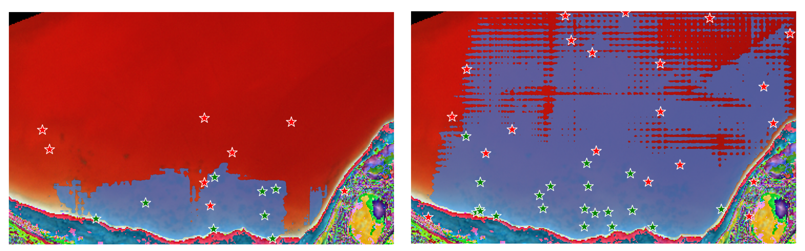
Examples of the UVeg masks generated with the foundational model, SAM, can be seen in Figure 7 and Figure 8. Figure 7 showcases masks created from a UAV mission scene, while Figure 8 presents masks derived from a WorldView-2 satellite scene.

The inter-modality comparison results are given in

Table 2. Comparison results of the different ML methods for the three data sources based on sufficiently large training datasets (different for each data source). Methods with highest $F1$ score are in bold.

Modality	ML Method	Size of Training Set	Dataset Size	$\mathit{F}1$	$\mathit{U}\mathit{A}$	$\mathit{P}\mathit{A}$
UAV	Log Regr	10-fold CV	∼8M px	0.350	0.219	0.861
	RF	10-fold CV	∼8M px	0.576	0.415	0.941
	SAM	20 px pairs	∼8M px	0.842 *	0.957	0.751
World View 2	Log Regr	20-fold CV	∼400k px	0.340	0.207	0.956
	RF	20-fold CV	∼400k px	0.472	0.328	0.845
	SAM	8 px pairs	∼400k px	0.264	0.157	0.834
Sentinel-2	Log Regr	40-fold CV	∼14k px	0.184	0.103	0.890
	RF	40-fold CV	∼14k px	0.331	0.231	0.581

* The highest $F1$ score of $86.5\%\pm 4.0\%$, with corresponding $UA$ of $89.6\%\pm 5.8\%$ and $PA$ of $83.9\%\pm 4.8\%$, is achieved for UAV images using 40 positive/negative pairs of pixels for prompting the SAM model.

. For each method and modality, the performance from a sufficiently large training dataset size is demonstrated to facilitate the assessment of UVeg segmentation using the different data sources. Notably, the performance results for the Sentinel-2 data source using the foundational model SAM are not calculated due to its significantly poor performance, rendering any results meaningless or trivial.

Table 2 provides the comparative analysis of the three data sources using k-fold cross-validation. The table showcases the performance metrics obtained from the concatenated confusion matrices, which offer a robust evaluation of the models. Notably, different numbers of folds were utilized for each modality to address the variation in dataset sizes. The SAM method is assessed by resampling a fixed number of pixel pairs with replacement, and this process is repeated 500 times.

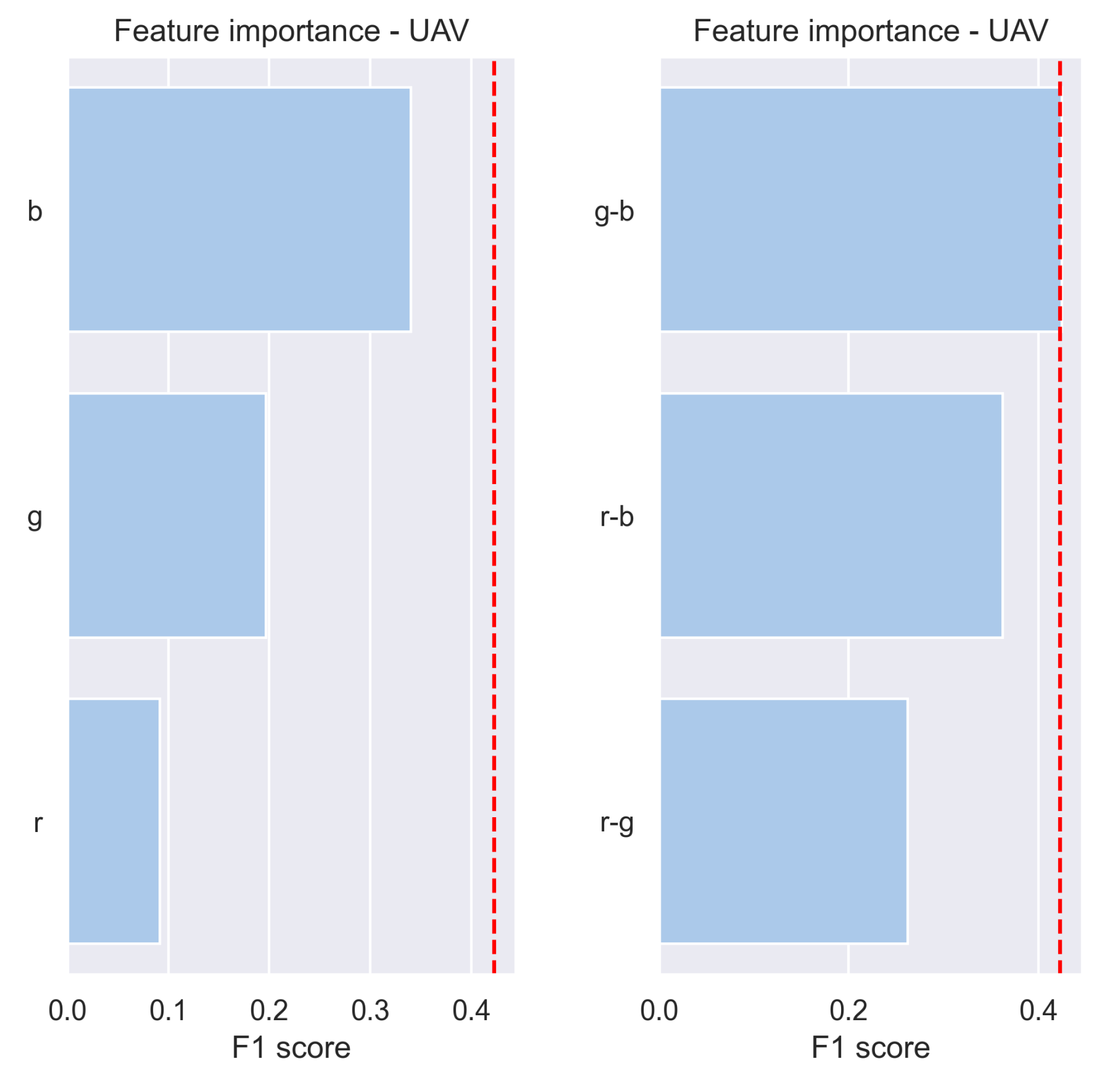
3.1. Feature-Importance Analysis

We further conducted a feature-importance analysis through an ablation study. By systematically removing specific bands and observing the resulting impact on model performance, we determined the significance of individual features in the context of single-feature, two-feature, and three-feature classifiers.

Figure 9, Figure 10 and Figure 11 present the outcomes of the feature importance analysis conducted on the three distinct data sources. The analysis evaluates the performance of single-feature, two-feature, and three-feature classifiers. The horizontal axis represents the feature importance score ($F1$ score), while the vertical axis displays the various features and representative feature combinations considered. These figures offer valuable insights into the diverse significance of features and their influence on model performance across different classifier configurations. The red dashed line denotes the baseline $F1$ score, computed based on all the features from each data source.

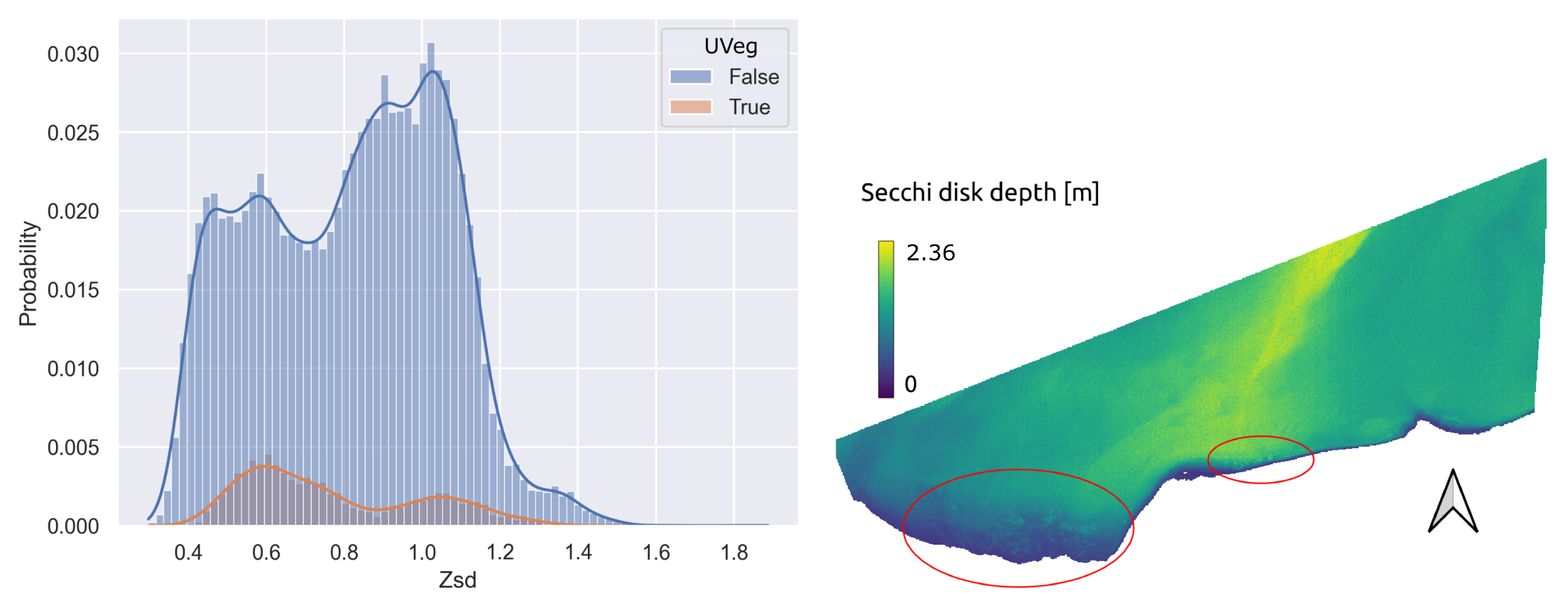
Figure 9 demonstrates the comparison results for the RGB bands of the UAV imagery. Figure 10 displays the comparison results for the eight bands of the WorldView-2 imagery, along with a separate panchromatic channel and a synthetic channel estimating the Secchi disk depth, as calculated from the QAA-RGB algorithm [18]. Figure 11 exhibits the comparison results for the 12 bands of the Sentinel-2 L2A products. Finally, a closer investigation into the Secchi disk depth synthetic feature based on the RGB bands of the WorldView-2 imagery for separating UVeg pixels is shown in Figure 12.

For reasons of practical interest, the feature importance analysis of WorldView-2 was also performed, apart from the total amount of pixels, on a subset of the image that exhibited a higher density of visually apparent UVeg regions and was close to the shore, which we thus consider “shallow pixels”. In Figure 10, the feature importance analysis of the complete image is shown in a light blue color, similarly to the analyses of UAV and Sentinel-2 imagery, while the analysis of the “shallow pixels” only is presented in gray. The UVeg segmentation baseline $F1$ scores using logistic regression with all bands for both groups (all pixels/shallow water only) are shown in red dashed lines.

3.2. Segment Anything Model Variants

Figure 13 provides a comparative analysis of two variants of the Segment Anything Model (SAM)—the “huge” and “base” versions. The comparison is conducted under a “few annotations” regime, where the number of positive/negative pair annotations is limited. The X-axis represents the number of annotated pairs, while the Y-axis denotes the $F1$ score. The mean values of the $F1$ score are accompanied by the standard deviation, indicating the variability in the model’s performance across multiple runs. This comparison is based on a bootstrap simulation conducted 500 times, providing a robust statistical analysis of the performance difference between the two SAM model variants.

3.3. Different Quantization in Sentinel-2 Pixels (Two to Four Classes)

In the context of applying multi-class classification to the Sentinel-2 data source, we present two significant figures. Figure 14 illustrates the class distribution of the quantized annotation at a GSD of 10 m, showcasing the complexity and possible class imbalance in the dataset. Figure 15 further explores the impact of different class granularities (two to four classes) on the data representation at the same GSD. These figures collectively offer insights into the challenges and implications of multi-class classification tasks within the Sentinel-2 data source.

3.4. Transferring UAV Models in Different Lake Areas

Table 3. Transferability of models in different lake locations using UAV data source. This table presents the results of evaluating the transferability of models across different locations within the lake. The logistic regression and random forest models were trained on AOI1 and tested on AOI2 and AOI3.

Data Source	Test Area	Test Area Size	ML Method	$\mathit{F}1$	$\mathit{U}\mathit{A}$	$\mathit{P}\mathit{A}$
UAV trained on AOI1	AOI 1 * (10-fold CV)	∼8 M px	LogReg	0.350	0.219	0.861
			RF	0.576	0.415	0.941
	AOI 2	∼8 M px	LogReg	0.312	0.228	0.493
			RF	0.291	0.291	0.292
	AOI 3	∼17 M px	LogReg	0.384	0.256	0.764
			RF	0.342	0.279	0.442

* Baseline results from Table 2.

presents the results of model transferability across different lake locations. The logistic regression model and random forest model were trained on AOI1 and evaluated on AOI2 and AOI3. The random forest model underwent hyperparameter tuning using Bayesian optimization with a validation set from AOI1.

4. Discussion

The results in Figure 4 demonstrate the superiority of the pre-trained foundation model, SAM, in the few-shot learning regime, i.e., limited annotations of positive and negative pixel-pairs for segmenting UVeg from UAV imagery. The highest $F1$ score of $86.5\%\pm 4.0\%$, with a corresponding $UA$ of $89.6\%\pm 5.8\%$ and $PA$ of $83.9\%\pm 4.8\%$, is achieved for UAV images using 40 positive/negative pairs of pixels for prompting the SAM model. The corresponding assessment metrics are much lower for the RF and logistic regression models, i.e., $54.0\%\pm 9.2\%$ using RF models and $42.8\%\pm 6.2\%$ using logistic regression models. The baseline $F1$ score for the UAV images is $42.3\%$ (red dashed line), which is the best linear separator of the UVeg/no UVeg classes based on the three bands R, G, and B of the UAV images.

In general, the baselines marked with red dashed lines in Figure 4, Figure 5 and Figure 6 serve as effective linear separators for all bands within each data source, considering the limited size of the available dataset. Consequently, we consider these baselines as valuable indicators of the information contributed by each modality in segmenting underwater aquatic vegetation.

A more comprehensive comparison of the three data sources based on different ML methods and sufficiently large training datasets (specific to each data source) is presented in Table 2. The methods with the highest $F1$ scores are highlighted in bold. Notably, the SAM method performs best for the highest-resolution UAV imagery, while the random forest pixel-wise method remains the state of the art for the WorldView-2 and Sentinel-2 data sources.

We believe that the inability to adapt SAM to lower-resolution remote sensing images can be attributed to the specific characteristics of the training data used for the foundation model. To support this argument, we attempted simple methods like upsampling and patch splitting for WorldView-2 and Sentinel-2 images to generate synthetic higher-resolution images, but without success. However, we firmly believe that future research efforts should focus on properly training and adapting foundational models for coarser-resolution remote imagery, such as Sentinel-2 and WorldView-2, given the available resources in terms of training data and computational power.

The choice of using RF as a comparison with the SAM foundation model was based on the well-established understanding that ensembling techniques tend to outperform more basic methods in machine learning. Random forest, being a bagging model, along with boosting models, has demonstrated superior performance compared to other ML approaches [11,12]. While deep learning has been successful in computer vision and remote sensing, we could not utilize such methods due to the limited annotated data for our task, making the foundation model the most suitable option. Additionally, we included logistic regression as a baseline ML method since it represents traditional thresholding techniques commonly used in remote sensing studies, where linear combinations of bands are designed.

In Figure 7, two masks were produced for the same scene captured during the UAV mission using three RGB bands. These masks were based on different random selections of eight prompt-input points, where the red stars denote negative class input points and the green stars indicate positive class input points. We observe the impact of the point-pair selection on the segmentation accuracy, with the segmentation mask on the left being more accurate than the one on the right, which can also be seen quantitatively in the model’s variance in Figure 4, with eight point-pairs. The number of point-pairs for this demonstration was selected because with eight pairs of positive/negative points the SAM model results in generally accurate masks; however, in some cases the model fails and results in masks like the one on the right of Figure 7. Investigating the impact of the input-point selection strategy in an active learning regime (interactively), e.g., selecting the most prominent errors of the current predicted mask, is an ongoing focus of our research group with significant practical applications.

In Figure 8, two additional masks were produced for a scene recorded by the WorldView-2 satellite. The three most informative bands (Green–RedEdge–NearInfrared1) were selected for this operation, as per the feature importance analysis discussed in Section 2. The left panel shows a mask created using eight pairs of positive/negative input points, which yielded the highest $F1$ score according to the results presented in Figure 5. Conversely, the right panel exhibits a mask that contains notable artifacts. These artifacts were more prominent when using a greater number of positive/negative point pairs, resulting in a reduction in performance, as evident in the findings displayed in Figure 5.

The feature importance analysis of the three data sources, as depicted in Figure 9, Figure 10 and Figure 11, was conducted through an ablation study. The analysis of the UAV bands using a single-feature classifier revealed that the blue band provides the most informative data, while the combination of green and blue bands, as a two-feature classifier, performed nearly as well as the baseline linear separation using all bands together. Regarding Sentinel-2 in Figure 11, the most informative bands for UVeg segmentation were found to be B07, B08, B01, and B09 when employing single-feature classifiers. Additionally, the combinations of B01-B07-B12 and B01-B07-B11 were demonstrated to encompass the complete information required for linearly separating pixels with UVeg presence.

In consideration of practical applications, due to the high cost of UAV imagery and the large GSD of the Sentinel-2 imagery, the WorldView-2 modality is considered a feasible choice for UVeg detection. Consequently, a more sophisticated feature importance analysis of WorldView-2 data was conducted that investigates the effect of pixels’ proximity to the shore in feature importance. Specifically, apart from the total amount of pixels, a feature importance analysis in Figure 10 was conducted on a subset of the image that exhibited a higher density of visually apparent UVeg regions and is close to the shore, which we thus considered “shallow pixels”. The areas of the lake further from the shore did not have visually apparent UVeg, probably because of the lake’s depth. In “shallow waters”, both the blue (B) and green bands (G) demonstrated high informativeness, whereas their significance diminished when considering the total amount of pixels due to the presence of deeper-water pixels. Despite B and G individually achieving the highest $F1$ scores in the single-feature classifier, the combination B-G did not result in further enhancement in the two-feature classifier. This can likely be attributed to the similarity in information content between both bands concerning UVeg segmentation, indicating that their combination does not yield better results. Moreover, the combination of green, red, and near-infrared1 bands encompassed almost the entire information content of all bands. Similar conclusions were drawn for the two- and three-feature classifiers, both for the “shallow water” subset and the complete image encompassing deeper waters. However, when examining the Secchi disk depth (Zsd) as a single-feature classifier, it exhibited poor discriminative power as a synthetic index computed by the QAA-RGB algorithm [18]. The lack of separability is further illustrated in Figure 12, where the histograms of the two classes are visually and quantitatively indistinguishable.

Figure 13 provides interesting insights into the performance of two SAM variants, “huge” and “base”. The SAM model has two encoder options: ViT-B (91M parameters) and ViT-H (636M parameters). While ViT-H is expected to show significant improvement over ViT-B, we noticed a surprising change in the $F1$ score and precision for around 100 positive/negative pixel pairs. These findings are intriguing and will guide our future research.

Based on our analysis of the Sentinel-2 data source in Section 3.3, it appears that increasing the granularity of the class structure from binary to multi-class models, namely, two- to four-class models, inversely impacts the accuracy of the classifications. As evidenced in Figure 15, the performance, when measured in terms of balanced accuracy, diminishes as we progress from binary to multi-class classification. Furthermore, the class distribution depicted in Figure 14 underscores the significant data imbalance at a GSD of 10 m. This class imbalance might contribute to the decrease in model performance as the class granularity increases, as the models may struggle to learn from under-represented classes. Interestingly, this pattern holds consistently across different time periods, underscoring the robustness of these observations and contributing insights to the optimal approach to classifying complex, multi-dimensional datasets like those derived from Sentinel-2.

The results in Table 3 show comparable metrics for the different AOIs, thus clearly demonstrating the ability of the logistic regression models to be successfully transferred to different locations within the lake. The results based on the random forest pixel-wise classifier show a reduction in all metrics compared to the cross-validation baseline, which is attributed to the limited dataset size of the cross-validation study in AOI1. Although all AOIs were captured on the same date in a single UAV mission (as shown in Table 1), these findings provide valuable insights into the practical usage of such models. For example, during a UAV mission covering the entire lake, it would be feasible to segment all UVeg regions by training or fine-tuning a model on a smaller subarea and then transferring the trained model to the rest of the lake. No results are provided for the Segment Anything model due to insufficient data for fine-tuning; however, recent studies propose methods for adapting prompts with one shot [22].

Considering the successful transferability observed with the logistic regression model in Section 3.4, a potential direction for future research would be to explore adapting the Segment Anything model to new lake areas. Building upon the insights gained, incorporating the one-shot prompt adaptation methods proposed by Zhang et al. [22] may enable the transfer of the Segment Anything model’s capabilities. This could facilitate the efficient segmentation of UVeg regions across larger areas of the lake, even on different dates, by leveraging a fine-tuned model from a smaller subarea.

5. Conclusions

In summary, this work demonstrates the effectiveness of the SAM foundation model for segmenting underwater vegetation in high-resolution UAV imagery in the few-shot learning regime. However, adapting SAM to lower-resolution images (WorldView-2 and Sentinel-2) remains challenging, and traditional pixel-wise methods remain the state of the art in our task. The specific characteristics of the foundation model training data are believed to be the reason for this inability to adapt SAM, despite attempts with techniques like patch splitting and upsampling.

The feature importance analysis and comparison of ML methods across the three data sources reveal important insights. The analysis of single-feature classifiers highlights the significance of specific bands in each data source and the limitations of synthetic indices like the Secchi disk depth. These findings provide valuable guidance for future research and practical applications in underwater vegetation segmentation.

Additionally, the study explores SAM variants and the impact of class granularity on Sentinel-2 classification. Logistic regression models demonstrate successful transferability across different areas within the lake, offering a practical approach to segmenting UVeg regions in larger areas using models trained on smaller subareas. Future research can focus on adapting the Segment Anything model to new lake areas using one-shot prompt-adaptation methods, facilitating efficient segmentation across larger areas and different dates.