Soil Moisture Monitoring and Evaluation in Agricultural Fields Based on NDVI Long Time Series and CEEMDAN

Abstract

The North China Plain is an important area for agricultural economic development in China. But water shortages, severe groundwater over-exploitation and drought problems make it difficult to exercise the topographic resource advantages of the plain. Therefore, the precise monitoring of soil moisture is of great significance for the rational use of water resources. Soil characteristics vary in natural farmland ecosystems, crops are constrained by multiple compound stresses and the precise extraction of soil moisture stress is a difficult and critical problem. The long time series was decomposed via complete ensemble empirical mode decomposition with adaptive noise (CEEMDAN) to obtain different intrinsic mode function (IMF) components, and the statistical descriptors of each component were calculated to realize the precise discrimination of soil moisture stress. A quantitative evaluation model of soil moisture was established, and the different noise addition ratios and modeling types were set respectively to investigate the optimal inversion model. The results showed that: (1) The reconstruction error of the CEEMDAN was small and almost 0; it had a high reconstruction accuracy and was more suitable for the decomposition of the long time series. The first two components, IMF₁ and IMF₂, were soil moisture stress subsequences, and it could effectively reflect the moisture stress situation. (2) The inversion model performed well when ε was 0.05 and the model type was quadratic, with a coefficient of determination R² of 0.98, which gave a better fit and less error. (3) The overall soil moisture content in the study area was low, basically in the range of 6.9% to 15.7%, with the central part, especially the south-central part, being the most affected by soil moisture stress, and the overall impact of soil moisture stress showed a decreasing trend from February to May. The utilization of CEEMDAN further enhances the accuracy of soil moisture inversion in agricultural fields, realizing the effective application of remote sensing observation technology and time-frequency analysis technology in the field of soil moisture research.

1. Introduction

Soil moisture is the material basis for the survival and growth of crops [1,2,3]. The absorption and transportation of nutrients by crops can only take place with the participation of soil moisture, which is an indispensable medium for chemical, biological and physical processes within the soil [4,5]. The phenomenon through which growth is restricted due to insufficient soil moisture during the reproductive period and the water is absorbed from the soil is not sufficient to support the normal physiological needs of the crop and is known as soil moisture stress [6]. Soil moisture stress on crops affects the vertical distribution of the root system, reducing the absorption capacity of the root system [7], and it affects the mineralization of soil fertility, reducing the performance of soil fertility. Therefore, the precise evaluation of soil moisture content is particularly important to the rational utilization of farmland water resources and the development of water-saving agriculture. The soil environment in natural farmland ecosystems is complex, and crops are affected by multiple compound stresses [8,9], for example, soil moisture stress, soil heavy metal stress and soil fertility stress. Among them, soil fertility stress has relatively stable inter-annual variability, while the heavy metal contamination of soil is irreversible; both of them are long-term stresses. In contrast, soil moisture stress is characterized by transient changes and is a short-term stress component. As the stressors are interactive and concomitant, it is crucial to accurately discriminate soil moisture stress during crop growth.

Remote sensing data are updated frequently and have spatial coverage continuity, fully reflecting the significant advantages of remote sensing technology in large-area dynamic real-time monitoring, and they have become the mainstream technical means of environmental monitoring [10]. The microwave remote sensing method is not easily influenced by the atmosphere, which has the advantage of functioning all day long, and its penetration ability is good, but its spatial resolution is limited and is disturbed by vegetation and surface roughness [11]. The thermal infrared remote sensing method makes full use of the daily variation of surface temperature, apparent thermal inertia and the thermal model to estimate the soil moisture content, but it is mainly suitable for the early stage of crop growth, low vegetation cover or bare ground, and it is affected greatly by meteorological conditions [12]. The optical remote sensing methods have the advantage of high spatial resolution and wide coverage, and they are more suitable for areas with a high vegetation cover [13]. There have been a large number of studies based on the vegetation index long-time series data of optical remote sensing images to achieve moisture monitoring. Liu Shiliang and others analyzed the evolution of the vegetation cover in the Yunnan Province of China based on the normalized difference vegetation index (NDVI) to explore the relationship between regional vegetation changes and droughts [14]. The NDVI long time series extracted from remote sensing images are non-linear and non-smooth [15]; in them, the information of diverse time characteristics and frequency characteristics are mixed. However, the studies on the time–frequency decomposition of NDVI long time series data for stress identification and extraction are relatively few, and few studies have successfully achieved the adequate removal of other stresses in the analysis of soil moisture, resulting in certain errors in soil moisture inversion. It is important to firstly separate the influence of multi-source and complexity factors on the NDVI long time series, remove the interference of other stressors and extract specific time-scale features, which is an important step in the accurate inversion of soil moisture for long time series vegetation index data. Signal processing, particularly signal processing methods with adaptive non-linearity [16], is required to achieve the extraction of specific features, decompose the vegetation index series and extract the components characterizing the specific features.

The Fourier transform (FT) represents continuous functions as linear combinations or integrals of sinusoidal basis functions, reducing the difficulty of processing the original signals [17,18]. Related studies [19,20] have applied FT to the classification of remote sensing images and the extraction of crop planting areas and obtained good results. The sinusoidal basis function in the FT is determined via the amplitude and initial phase, and the subjectivity of the threshold selection in the threshold method can be overcome using the cluster analysis of the basis function features. But FT can only obtain the global characteristics of the time series signal in the frequency domain, and it is difficult to analyze the specific frequency components of the signal in different time scales. To solve the above problem, the short time Fourier transform (STFT) was developed to analyze the spectral differences at different time scales and obtain the time-varying characteristics of long time series signals [21]. However, the use of remote sensing long time series for coercive discrimination requires different temporal and frequency resolutions of the signals at different time scales, and the STFT cannot find suitable time window functions to suit the characteristics of the signals at different time scales. The wavelet transform (WT) differs from the STFT in that its time–frequency window is not uniformly distributed in the phase plane, and its unique multi-scale and multi-resolution characteristics create a unique advantage for signal composition analysis [22,23,24,25,26,27]. But once the wavelet basis function is determined, the distribution of the time–frequency window in the time–frequency plane is then fixed with poor adaptability [28,29,30,31]. The above algorithms achieve the time–frequency decomposition analysis of long time series data, but none of them have good adaptive properties.

The Hilbert–Huang transform (HHT) is a signal decomposition algorithm for nonlinear and non-stationary signals, including the empirical mode decomposition (EMD) algorithm and Hilbert spectral analysis [32,33,34]. The HHT algorithm does not require a pre-set basis function and has the advantages of intuitiveness a posteriori and adaptiveness, which are the most essential differences compared with the FT, STFT and WT algorithms. The EMD algorithm can decompose the original long time series into a number of single-frequency sequences and a residual component by adaptively separating out the data sequences at different scales from the signal to be decomposed and obtaining the intrinsic mode function (IMF) under certain conditions [35]. The fluctuation characteristics of each IMF component will change with the signal itself, the IMF components can be extracted more accurately according to different time scales and different characteristic information on each time scale can be analyzed [36].

The EMD algorithm has been widely used in the study of temporal signal decomposition [37,38]. But EMD decomposition can produce the phenomenon of modal confusion, for which a large number of scholars have improved the EMD. Huang E and others proposed ensemble empirical mode decomposition (EEMD), which adds several times of Gaussian white noise signals to the original long time series and combines the two as a new approach to decomposition using the property of Gaussian white noise in the frequency domain to obtain the closest realistic modal component after several averaging calculations [39,40,41]. Nevertheless, a small amount of noise remains in the decomposed IMF components of EEMD, which affects the subsequent signal processing and analysis. In order to solve the above-mentioned modal mixing and noise residual problems, Torres et al. put forward an improved algorithm, namely complete ensemble empirical mode decomposition with adaptive noise (CEEMDAN) [42,43,44]. CEEMDAN will add adaptive white noise to each decomposition process, and after the first order IMF component is obtained, the overall average calculation will be performed as the final first-order IMF component, and only the unique IMF remainder will be generated [45,46], solving the problem of noise transmission.

In addition, most studies have used traditional methods such as multiple linear regression, typical correlation analysis and principal component analysis for model construction and analysis. But there are problems, such as inaccurate parameter estimation among multiple variables, which leads to the inaccurate inversion of soil moisture when the independent variables are multiply autocorrelated. Partial least squares regression (PLSR) decomposes and filters all the data [47]. Firstly, the principle of principal component analysis is used to condense and synthesize the variable indicators; then, it analyses the relationship between the original variables and the composite variables with the help of the principle of typical correlation and extracts the composite variables that best explain the dependent variable. Finally, the relationship between independent variables and dependent variables is analyzed based on the principle of multiple linear regression, and the advantages of each method are combined for model construction. However, few studies have used the CEEMDNA and PLSR for the remote sensing of soil moisture stress screening and inversion.

Taking into account the non-linearity and non-smoothness of the NDVI long time series, the excellent decomposition performance of CEEMDAN and the advantages of PLSR in multi-metric modeling, this paper proposes a method to monitor and evaluate soil moisture in agricultural fields based on the CEEMDAN–PLSR algorithm to achieve the accurate discrimination of soil moisture stress and accurate inversion of soil moisture content. The innovations and possible contributions could be summarized as follows:

(1)

A new soil moisture content inversion model was constructed by combining the CEEMDAN with the PLSR algorithm, and the model has better accuracy and stability, providing a new solution for real-time and accurate soil moisture monitoring;

(2)

The CEEMDAN algorithm is applied to the screening and extraction of soil moisture stress, developing the application of CEEMDAN in the field of soil moisture research. CEEMDAN can effectively decompose the NDVI long time series and accurately extract the characteristic components of soil moisture stress, making the inversion results more accurate;

(3)

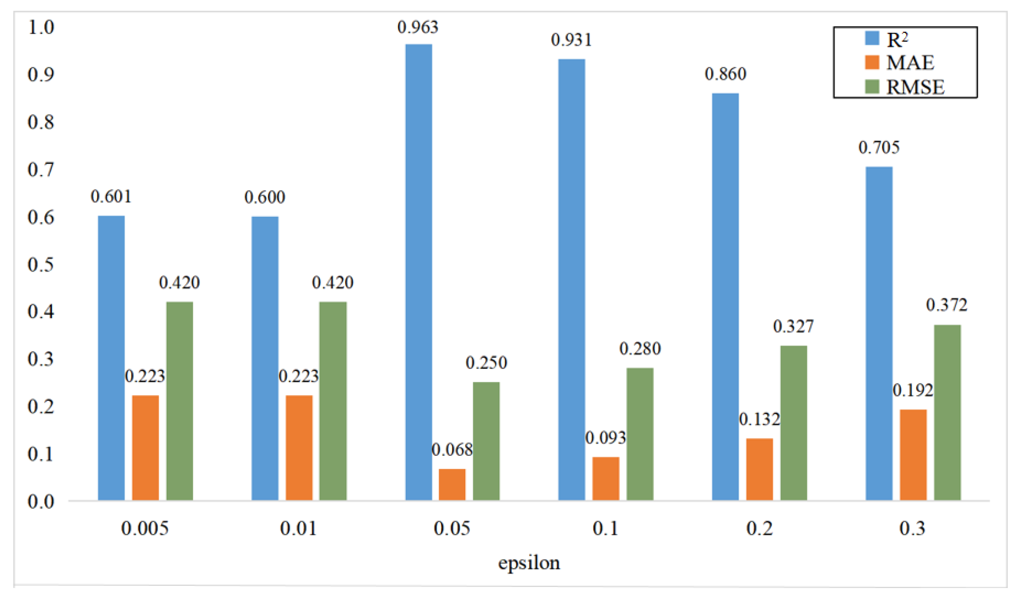
The optimal decomposition parameter epsilon of CEEMDAN and the optimal inversion model type of PLSR were determined experimentally, and the optimal inversion model based on CEEMDAN and PLSR for soil moisture content inversion was explored to further improve its generalization capability and accuracy;

(4)

The effective inversion of soil moisture content and the analysis of spatiotemporal distribution characteristics in the study area were completed based on the optimal inversion model, providing a scientific basis for drought management and agricultural planning.

2. Materials and Methods

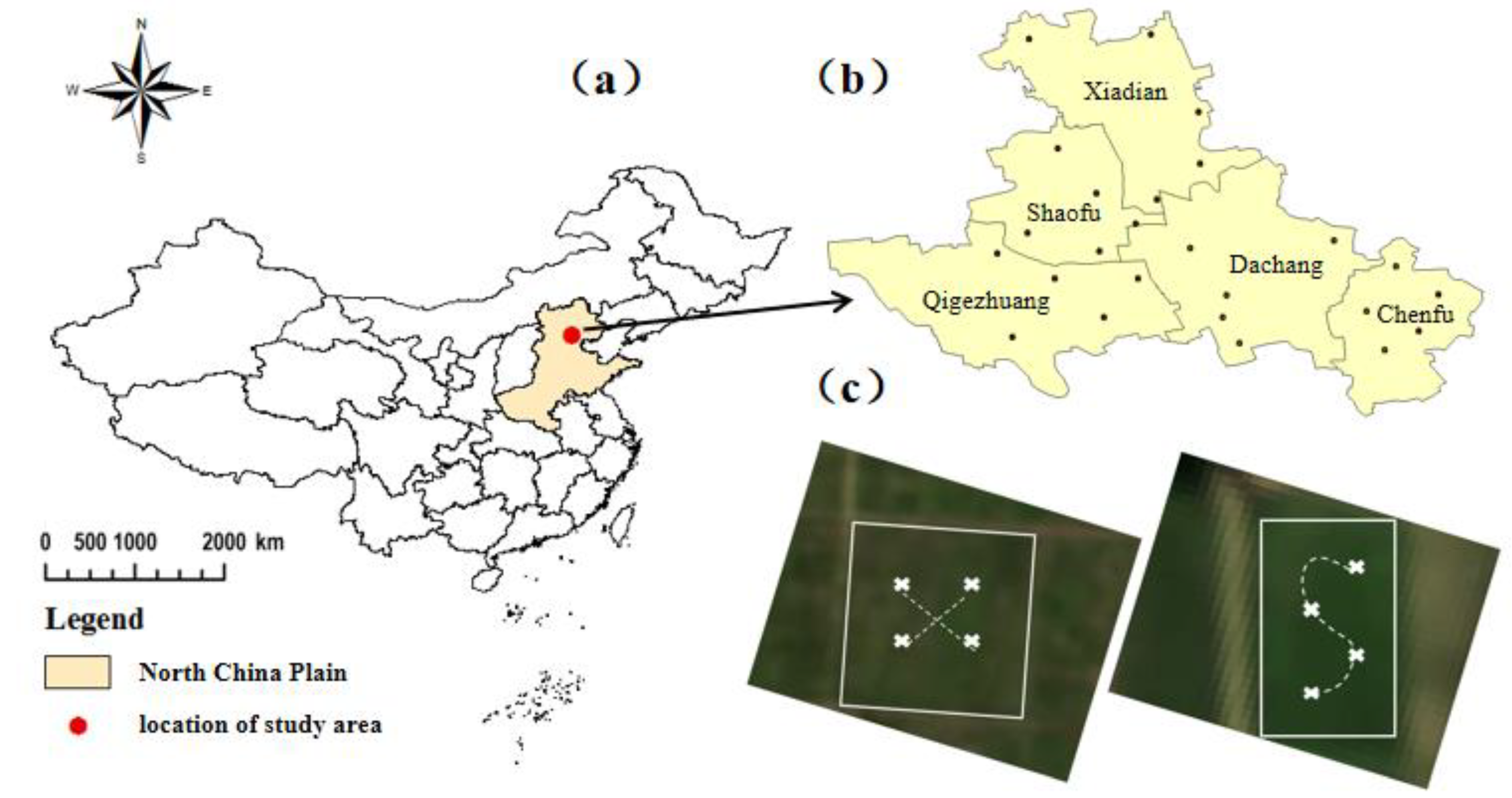
2.1. Study Area

The North China Plain is flat and well cultivated, and as of 2021, its area had reached 310,000 km². The plain accounts for more than 18% of the yield of grain in China and is an important base for grain, cotton and oil production in China [48]. However, water resources in the plain are scarce, and it is the world’s largest underground water leakage area, of which most of the leakage area is again concentrated in Hebei Province. The leakage area in Hebei Province is about 40,000 km², causing water scarcity, with the amount of water resources available in the province far below the total water consumption. This water scarcity has led to the over-extraction of groundwater, and around 75% of the groundwater extracted in Hebei Province is actually used for the irrigation of farmland. Therefore, a reasonable way to monitor the soil moisture content of farmland in real time and to accurately ensure the agricultural water resources and winter wheat yield in the North China Plain is a topic of great importance for food security and sustainable development. Dachang Hui Autonomous County, Hebei Province, is located in the North China Plain and produces wheat and maize, making it one of the major grain producers in the plain. However, heavy industries such as cement enterprises in Hebei Province are distributed in most of the cities and towns; heavy industrial enterprises have less disposal of soil heavy metal pollutants [49], and the effective phosphorus and fast-acting potassium fertility nutrient content in farmland is relatively low [50]. In addition to soil moisture stress, there are a certain heavy metal stress and a fertility stress in the soil.

2.1.1. Geographical Location and Landforms

Dachang Hui Autonomous County is located directly east of Beijing, with an area of 176 km². Dachang is located at the southern foot of Yanshan Mountain, and it is influenced by the North Canal in the west and southwest and the Chaobai River in the east and southeast, with a wide alluvial plain that is high in the northwest and low in the southeast, which is very suitable for farmland food cultivation.

2.1.2. Climate and Vegetation Characteristics

Dachang Hui Autonomous County has a warm, temperate, semi-humid continental monsoon climate that is dry and windy in the spring, hot and rainy in the summer, mild and cool in the autumn and cold and dry in the winter. With an average annual temperature of 11.4 °C and an annual sunshine duration of 2853.2 h, the local area has very favorable light and heat conditions for crop growth, especially for wheat and maize. The county belongs to the crop cultivation area of the North China Plain, where field crops are the most important terrestrial vegetation and are most widely distributed, mainly of the winter wheat and maize crop rotation type, with winter wheat mainly from October to early June of the following year. The average annual precipitation is 554.9 mm, and the distribution of precipitation varies unevenly with the seasons, with natural precipitation generally unable to meet the growth needs of winter wheat.

2.1.3. Hydrological and Geological Profile

The stratum of Dachang Hui Autonomous County is the Quaternary Holocene, which is a river- and lake-phase sedimentary layer dominated by river and mountain flooding sub-sand and sub-clay powder and fine sand. The grain size of the soil layer gradually becomes coarser from top to bottom, containing calcareous nodules. The geology is powder clay, and the water gathering and seepage are not fast. The groundwater flows from the northwest to the southeast, and the shallow groundwater mainly receives recharging from atmospheric precipitation; its quality is poor, and it is easily polluted, not suitable for drinking and only suitable for industry and agricultural irrigation.

In this study, Dachang Hui Autonomous County in Hebei Province was taken as the study area (Figure 1a), and the five townships under the jurisdiction were used as the five sampling scopes. Five representative typical winter wheat planting plots with obvious features were selected within each sampling scope (Figure 1b). The four sampling points were kept a certain distance away from the ridge and the edge of the field. An X-shaped sampling method was adopted when the plot was closer to a square, and an S-shaped sampling method was adopted when the plot was closer to a rectangle (Figure 1c). The sampling points for the ground data were consistent with the vector information of the sampling points for NDVI extraction, and the data were measured and collected for each of the five critical fertility periods of winter wheat.

2.2. Data Sources

2.2.1. Remote Sensing Data

The acquisition of NDVI long time series data requires high requirements for the satellite launch time and the cloudiness of images. This study gave priority to GF-1 images with less than 5% cloud coverage, and Landsat 8 image data were alternately used when the GF-1 images showed cloudy coverage in the study area. Considering the resolution, the Landsat 7 digital product provided support for image data before March 2013. Finally, data from 120 scene images from January 2012 to December 2021 were selected to construct the NDVI long time series in a monthly cycle.

GF-1 WFV images were pre-processed through three steps, as follows. The scale factor was taken as 0.1 to complete the radiation calibration. The date, time and resolution of the images were automatically acquired according to the images’ information. The atmospheric model was selected in conjunction with the month of each image. The rural aerosol model was selected. The spectral response function was selected according to different sensor models, and the other parameters were kept as defaults to complete the atmospheric correction. The output pixel size was set to 16. The cubic convolution method was chosen for image resampling, and all other parameters were left as default to complete the orthorectification. And finally, the NDVI was calculated for the output image of geometric corrections.

Landsat 8 images were pre-processed through five steps of radiometric calibration, atmospheric correction, image sharpening and resampling, and then they were registered with the GF-1 image as the reference. Finally, the NDVI was calculated. During atmospheric corrections, the right atmospheric model was selected according to the image month. The images were fused using the Gram–Schmidt pan sharpening tool, selecting the multispectral data file first and then the panchromatic data file for fusion, and in the pan sharpening parameters panel, the sensor selected was landsat8_oli and the resampling selected was cubic convolution. The resampling resolution was set to 16, which was the same as the GF-1 image resolution. Finally, NDVI was calculated for the aligned images. Unlike Landsat 8 images, Landsat 7 images were downloaded with missing data strips, requiring strip repair. The study first used the landsat_gapfill plug-in in ENVI to repair the missing strips and then performed the same five steps for Landsat 8 and also the NDVI calculation.

The ArcGIS 10.2 software platform was used to generate the sample area vector files and extract NDVI data based on all the pre-processed image data. Firstly, multi-value extraction was used as the point tool during the spatial analysis, the vector file was selected as the input point element, all image data were selected as the input raster data and the NDVI values were saved to the vector attribute column. Then, the table to Excel tool under conversion tools was selected, the vector file was selected as the input table, the output Excel file path name was set, the extracted NDVI data were exported and the NDVI long time series was constructed in time as the horizontal coordinate.

2.2.2. Ground-Measured Data

The impact of soil moisture stress on crops is mainly reflected in changes in the relevant growth indicators. There are various indicators that reflect crop growth, such as leaf chlorophyll content, plant water content and plant height, etc. The selection of indicators in this paper was based on two main principles, relevance and consistency, the first of which was relevance. In general, the higher the correlation between the growth index and soil moisture, the better the index will be able to characterize the degree of response to soil moisture stress. For example, plant height, though also influenced by soil moisture, can to some extent reflect the growth of winter wheat and its response to soil moisture stress, but its variation is mainly in response to soil fertility and is less correlated with soil moisture. Meanwhile, with the advancement of technology and in order to avoid an excessive plant height, winter wheat varieties are resistant to overturning, plant height is influenced by a variety of factors, and the differences in the effect of different levels of soil moisture stress on the height of winter wheat plants was not significant and was excluded from the selection of indicators. Secondly, for consistency, the selected indicators needed to meet the requirements of both reflecting crop growth and responding to soil moisture stress. This means that the selected indicators reflected both changes in growth and a consistent response to changes in soil moisture content. The chlorophyll content, plant moisture content and soil moisture were in good agreement, and the chlorophyll content was significantly reduced via soil moisture stress, which limited the accumulation of dry matter in winter wheat and affected the plant moisture content. In summary, three indicators were selected: chlorophyll content, plant water content and soil water content. We collected leaf chlorophyll content, winter wheat plant samples and soil samples during five critical fertility periods of winter wheat in 2021. The details of each stage are shown in

Table 1. Five critical fertility periods.

Stage	Duration	Sample Time	Characteristics
Jointing stage	Mid-March to early April	4 April	The internodes above the ground grew about 2 cm and exhibited relatively low water consumption.
Booting stage	Early April to mid-April	17 April	All leaves extended out of the leaf sheath, and the water demand gradually increased.
Heading stage	Mid-April to early May	2 May	More than half of the tops of wheat ears had leaf sheaths showing, and a lack of water could severely reduce yields.
Flowering stage	Early May to mid-May	13 May	More than half of the wheat ears bloomed, and they had relatively high water requirements.
Filing stage	Mid-May to early June	25 May	The plant moisture content rapidly increased, and dry matter accumulation tended to be at its maximum.

. To ensure accurate and scientific results, each collection was completed between 8 a.m. and 12 a.m. Of the resulting ground truth data, 75% was used for model construction and the remaining 25% for accuracy validation.

(1)

Relative chlorophyll content determination

The relative chlorophyll content in the leaves of winter wheat plants was measured using a handheld chlorophyll tester. The handheld chlorophyll tester used in this paper was the LD-YC model. The measuring area was 2 mm by 2 mm, the maximum sample thickness was 1.2 mm and the maximum sample insertion depth was 12 mm. The light source was 2 LEDs, and the receiver was 1 SPD. The emission and reception windows of the handheld tester’s sample holder were checked before measurement to ensure that the sample holder window was clean. The measurements were carried out while avoiding the absolutely thick parts of the leaves, such as the veins. The leaves were measured from the top, middle and bottom 3 parts, and the average of the 3 parts was taken as the final value for each plant. The average of the 5 trials was taken as the final result for each sampling point.

(2)

Plant moisture content determination

The table-top vacuum drying oven of the SPRZK-20 model was used in this paper. Its display was a high-precision digital-display temperature-control instrument. The supply voltage was AC220 V 50 HZ. The temperature control range was from 10 to 200 °C at room temperature. The temperature resolution was 0.1 °C. The fluctuation was 1 °C up and down. Its input power was 800 W. The load tray was equipped with 2 pieces, as is standard. The complete winter wheat plants were dug up at the sampling site, and it was ensured that the sample was filled in the shortest possible time and taken back in a sealed bag to avoid water loss. After cleaning the impurities, absorbent paper was used to absorb water and weighed for fresh biomass (FB) using balance. The samples were then dried at 80 °C to a constant weight and weighed for dry biomass (DB), and the plant moisture content (PMC) was calculated.

$$\mathrm{PMC}=\frac{\mathrm{FB}-\mathrm{DB}}{\mathrm{FB}}\times 100\%$$

(1)

(3)

Soil moisture content determination

The lowest soil temperature during the test was 9 °C, and the lowest air temperature was 13.8 °C. The highest soil temperature was 22.1 °C, and the highest air temperature was 33.2 °C. There was no rainfall that occurred on the sampling day. The soil was dug within 5 to 10 cm of the sample point, and the plots that had just been irrigated were avoided as far as possible to avoid any human influence on the accuracy of the soil mass moisture content data and to ensure that the changed farm plots should be adjacent to the original sampling area farm plots. The soil samples were sealed and taken back to the laboratory and weighed on balance to obtain the fresh weight (FW). The oven temperature was set to 105 °C, and the soil was dried until its weight no longer changed. Then, it was weighed to obtain the dry weight (DW), and at last, the soil moisture content (SMC) was calculated.

$$\mathrm{SMC}=\frac{\mathrm{FW}-\mathrm{DW}}{\mathrm{DW}}\times 100\%$$

(2)

2.3. Methods

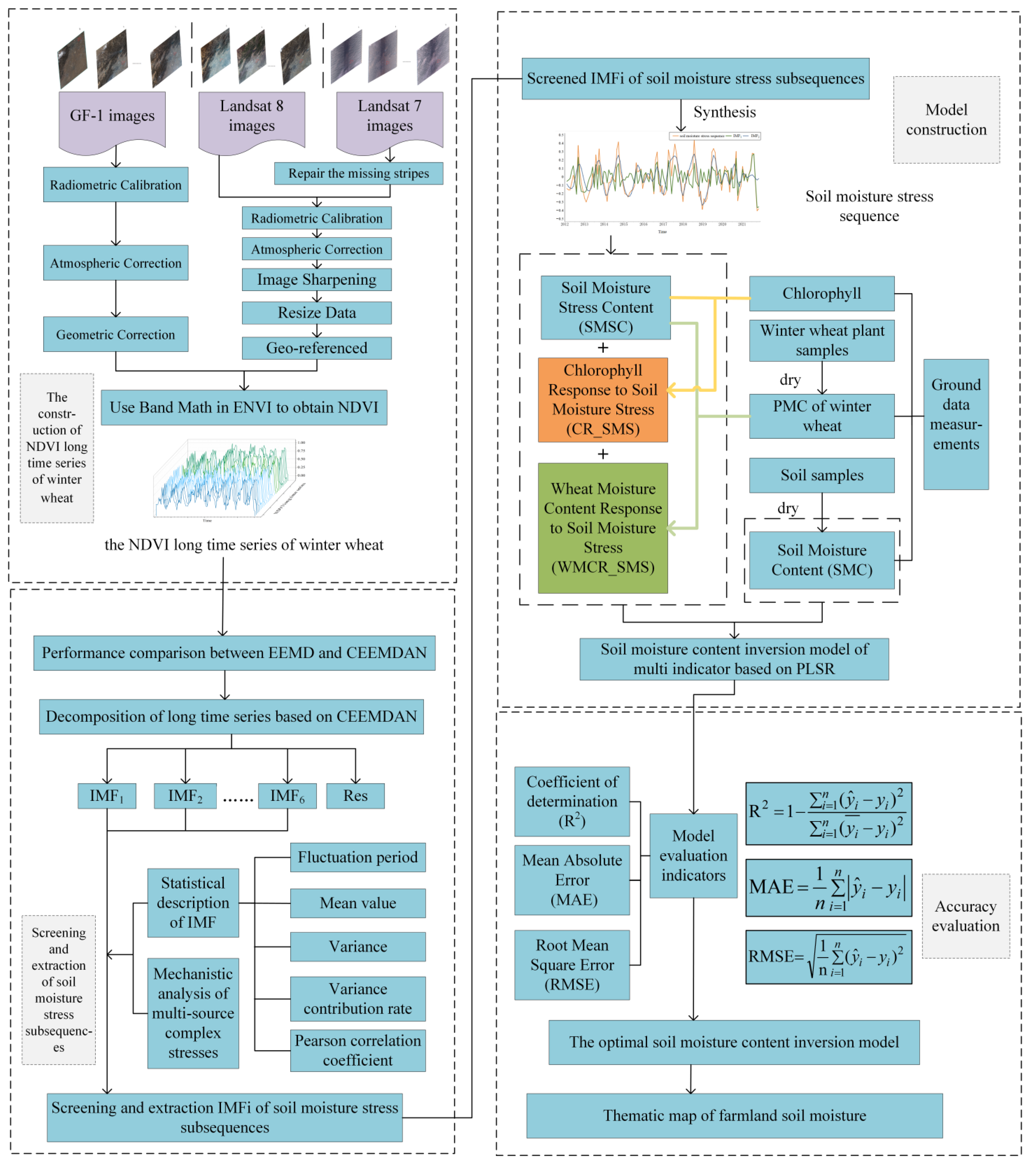
2.3.1. Technical Flow

In this research, the long time series of NDVI under a natural farmland ecosystem were constructed based on remote sensing data, and the decomposition effect and data reconstruction performance of the EEMD algorithm and the CEEMDAN algorithm were compared. Each IMF component was obtained via CEEMDAN decomposition; then, the fluctuation period, mean, variance, variance contribution and Pearson correlation coefficient of each component were calculated. The results of each IMF component were compared and analyzed, and the sub-series of soil moisture stress were extracted by combining the mechanistic characteristics of the soil moisture stress. Then, the soil moisture stress characteristic curve was fitted with the measured time to obtain the soil moisture stress content (SMSC), and the chlorophyll response to soil moisture stress (CR_SMS) and the wheat moisture content response to soil moisture stress (WMCR_SMS) indexes were constructed via a combination with the ground measurement data. The soil moisture content inversion model was constructed using PLSR, and the optimal decomposition parameters of the CEEMDAN algorithm were obtained by setting the ratio of added noise to 0.005, 0.01, 0.05, 0.1, 0.2 and 0.3, respectively, and comparing the inversion accuracy of the linear, quadratic and cubic modeling types to select the optimal inversion model, further completing the analysis of the spatial and temporal distribution characteristics of soil moisture content in the study area. The technical flow is shown in Figure 2.

2.3.2. EEMD and CEEMDAN

The EEMD algorithm continuously decomposed the original long time series into a number of single-frequency components and a residual component. However, EEMD still had the defect of noise transfer in the decomposed IMF components, which failed to minimize the impact of the signal decomposition on the later data analysis, resulting in the poor accuracy of the final results. The CEEMDAN algorithm added adaptive white noise to each decomposition of the signal and only generated a unique IMF component each time, solving the noise transfer problem and improving the adaptiveness of the algorithm. The fluctuation characteristics of each IMF component changed with the signal itself so that the corresponding IMF components could be extracted more accurately according to different time scales, and the different characteristic information on each time scale could be analyzed. The detailed decomposition process of CEEMDAN is summarized below.

Step 1: Determine the number of noise integrations M, add adaptive white noise $Z^{\left(m\right)}\left(t\right)$ to the NDVI long time series $X\left(t\right)$ to obtain the sequence $X^{\left(m\right)}\left(t\right)$ to be decomposed, and ${\epsilon }_m$ is the standard deviation of the mth addition of the noise.

$$X^{\left(m\right)}\left(t\right)=X\left(t\right)+{\epsilon }_m{Z}^{\left(m\right)}\left(t\right)$$

(3)

Step 2: The first IMF component of CEEMDAN is obtained by decomposing $X^{\left(m\right)}\left(t\right)$ several times and calculating the mean of the decomposition results.

$${\mathrm{IMF}}_1=\left(1/M\right){\displaystyle \sum _{m=1}^M{\mathrm{IMF}}_1^{\left(m\right)}}$$

(4)

${\mathrm{IMF}}_1^{\left(m\right)}$ denotes the IMF component obtained by EMD decomposition of the sequence $X^{\left(m\right)}\left(t\right)$ to be decomposed, and the remaining term $R_1\left(t\right)$ is obtained by subtracting the first IMF component IMF₁ from the original NDVI long time series $X\left(t\right)$.

Step 3: A new sequence $R_1\left(t\right)+{\epsilon }_m{E}_1\left(Z^{\left(m\right)}\left(t\right)\right)$ to be decomposed is obtained by superimposing adaptive white noise on the residual term $R_1\left(t\right)$, with $E_k(\cdot )$ denoting the kth component obtained via the EMD decomposition. The new sequence to be decomposed is then decomposed, and its mean value is found to obtain the second IMF component.

$${\mathrm{IMF}}_2=\left(1/M\right){\displaystyle \sum _{m=1}^M{E}_1\left(R_1\left(t\right)+{\epsilon }_m{E}_1\left(Z^{\left(m\right)}\left(t\right)\right)\right)}$$

(5)

Then, subtract the second IMF component IMF₂ from $R_1\left(t\right)$ to obtain the residual term $R_2\left(t\right)$.

Step 4: Repeat the above process to obtain the kth residual term $R_k\left(t\right)$ and the (k + 1)th IMF component ${\mathrm{IMF}}_{k+1}\left(t\right)$.

$$R_k\left(t\right)=R_{k-1}\left(t\right)-{\mathrm{IMF}}_k\left(t\right)$$

(6)

$${\mathrm{IMF}}_{k+1}\left(t\right)=\left(1/M\right){\displaystyle \sum _{m=1}^M{E}_1\left(R_k\left(t\right)+{\epsilon }_m{E}_k\left(Z^{\left(m\right)}\left(t\right)\right)\right)}$$

(7)

Step 5: The cycle is repeated until the residual term $R_k\left(t\right)$ can no longer be decomposed, and at last, a certain number of IMF components and a remainder term are obtained from the original long time series $X\left(t\right)$.

$$X\left(t\right)={\displaystyle \sum {\mathrm{IMF}}_i}+R\left(t\right)$$

(8)

2.3.3. Construction of the Soil Moisture Stress Response Index

Combining NDVI data to construct other vegetation indexes to synthesize the information of multiple index factors provides a solution to improve the soil moisture retrieval accuracy. In this research, the NDVI long time series was decomposed using the CEEMDAN algorithm to obtain the soil moisture stress subsequences, and the soil moisture stress subsequences were accumulated and synthesized to obtain the soil moisture stress sequence to characterize the effects of soil moisture stress on the growth cycle of winter wheat. Then, two points on the soil moisture stress sequence, including the time when the ground data were measured and the corresponding values, were fitted, and a linear fit was used to calculate the specific corresponding values for the time of measurement as the amount of soil moisture stress corresponding to the time of measurement.

CR_SMS used SMSC as the input variable and chlorophyll content as the output variable. We used various models, such as linear, quadratic curve, cubic curve and inverse models, the composite curve and the growth curve for curve estimation, and we selected the curve type with the best fitting index as the final fitting model for the subsequent CR_SMS calculation. Meanwhile, WMCR_SMS used SMSC as the independent variable and PMC as the dependent variable. In a way similar to the construction of CR_SMS, WMCR_SMS also used a different type of model as above for curve estimation and ultimately selected the curve type with the best fitting index as the final fitting model for the subsequent WMCR_SMS calculation. These two indicators were fitted separately as a function of the chlorophyll content and PMC, providing data and support to optimize the inversion model with the advantage of multiple indicators. The stress component data decomposed by the CEEMDAN algorithm were effectively fitted to the measured data, enabling the inversion process of obtaining stress response quantities based on remote sensing data and, at the same time, completing a key step in the quantitative inversion of soil moisture content.

2.3.4. Model Construction and Accuracy Evaluation

The PLSR algorithm can achieve multi-indicator model construction and elevate the accuracy and stability of inverse models. In recent years, it has received extensive attention in terms of methods, as well as applications, providing algorithmic support to achieve multi-indicator inverse model construction. The most significant difference between the PLSR algorithm and the principal component analysis method is that the PLSR algorithm considers the response matrix alongside the independent variable matrix, and the addition of the two matrices allows the PLSR algorithm to extract the best response to soil moisture stress and to cover the greatest amount of variation. It not only improves the identification of information and noise but also greatly reduces the influence of variable autocorrelation on model construction. In this paper, three variables, CR_SMS, WMCR_SMS and SMSC, were input variables, and SMC was the output variable to build the PLSR soil moisture content inversion model. The coefficient of determination (R²), the mean absolute error (MAE) and the root mean square error (RMSE) were used to evaluate the accuracy of the inversion model, and calculate the fitting error of the model. Using $y_1$, $y_2$, …, $y_n$ for truth, ${\widehat{y}}_1$, ${\widehat{y}}_2$, …, ${\widehat{y}}_n$ for the prediction value and n for samples, the formula for each index were as follows.

$${\mathrm{R}}^2=1-\frac{{\displaystyle {\sum }_{i=1}^n{({\widehat{y}}_i-y_i)}^2}}{{\displaystyle {\sum }_{i=1}^n{(\overline{y_i}-y_i)}^2}}$$

(9)

$$\mathrm{MAE}=\frac{1}{n}{\displaystyle \sum _{i=1}^n\left|{\widehat{y}}_i-y_i\right|}$$

(10)

$$\mathrm{RMSE}=\sqrt{\frac{1}{n}{\displaystyle \sum _{i=1}^n{({\widehat{y}}_i-y_i)}^2}}$$

(11)

3. Results

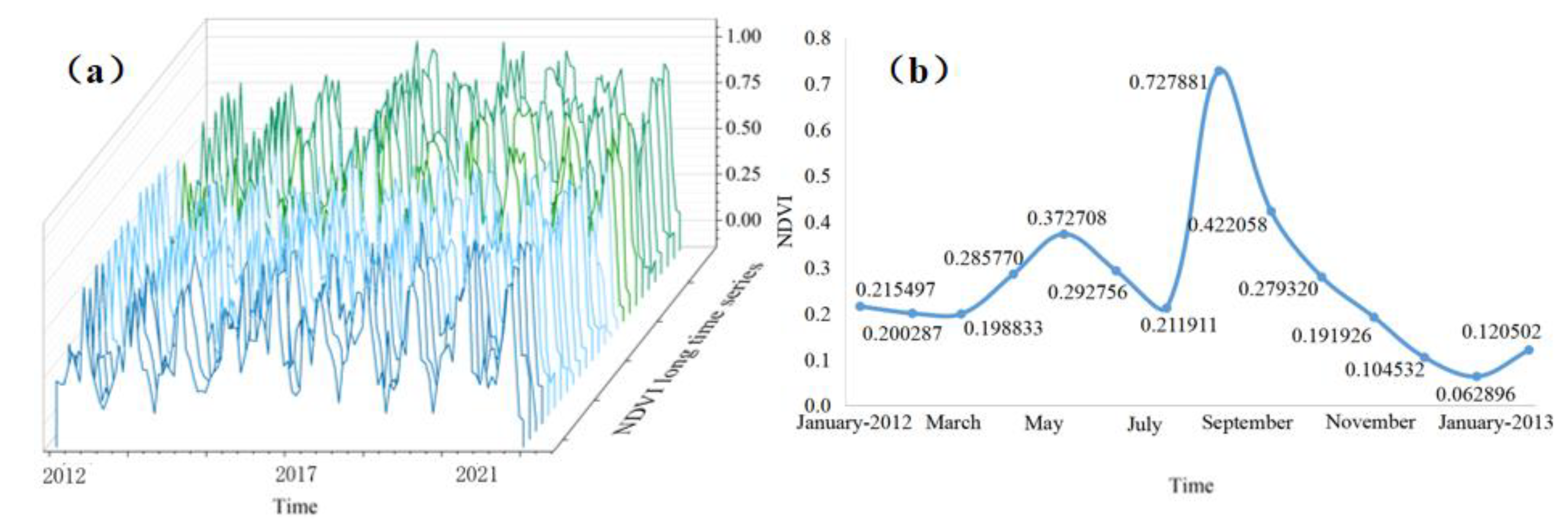
3.1. The NDVI Long Time Series

The NDVI long time series for winter wheat is shown in Figure 3a, and in the figure, the x-axis represents time, the y-axis represents different sampling points and the z-axis represents NDVI values. The NDVI value in the past 10 years changed with the change of vegetation coverage in different periods of time, and the monthly changes in different years were basically the same. The overall trend of the curve shows a certain periodic variation pattern in years. The trough of the NDVI value was basically concentrated between December and February, and the peak was basically concentrated between July and September. The NDVI value in the study area fluctuated between 0.1 and 0.9 in general. For different stages, NDVI was the lowest in the overwintering period (early December to early February), fluctuated moderately from rejuvenation to booting (mid-February to late April) and increased significantly from heading to filling (late April to mid-May). The NDVI values started to decrease significantly after the filling stage. In 2012, for example, as shown in Figure 3b, the value reached the highest of 0.37 in May and the lowest of 0.06 at the end of December. The NDVI long time series is the most intuitive way to reflect the NDVI fluctuation process of winter wheat from a multi-year macroscopic perspective, and the curve fluctuation shows a certain regularity, which is in line with the overall characteristics of the sawtooth double-peaked time series curve under the biannual cropping system in the research area. By decomposing the long time series of the crop, the different time scales and frequency characteristics help to eliminate the impact of other long-term noise factors, capture the transient characteristics of short-term components and further screen out the soil moisture stress subsequences.

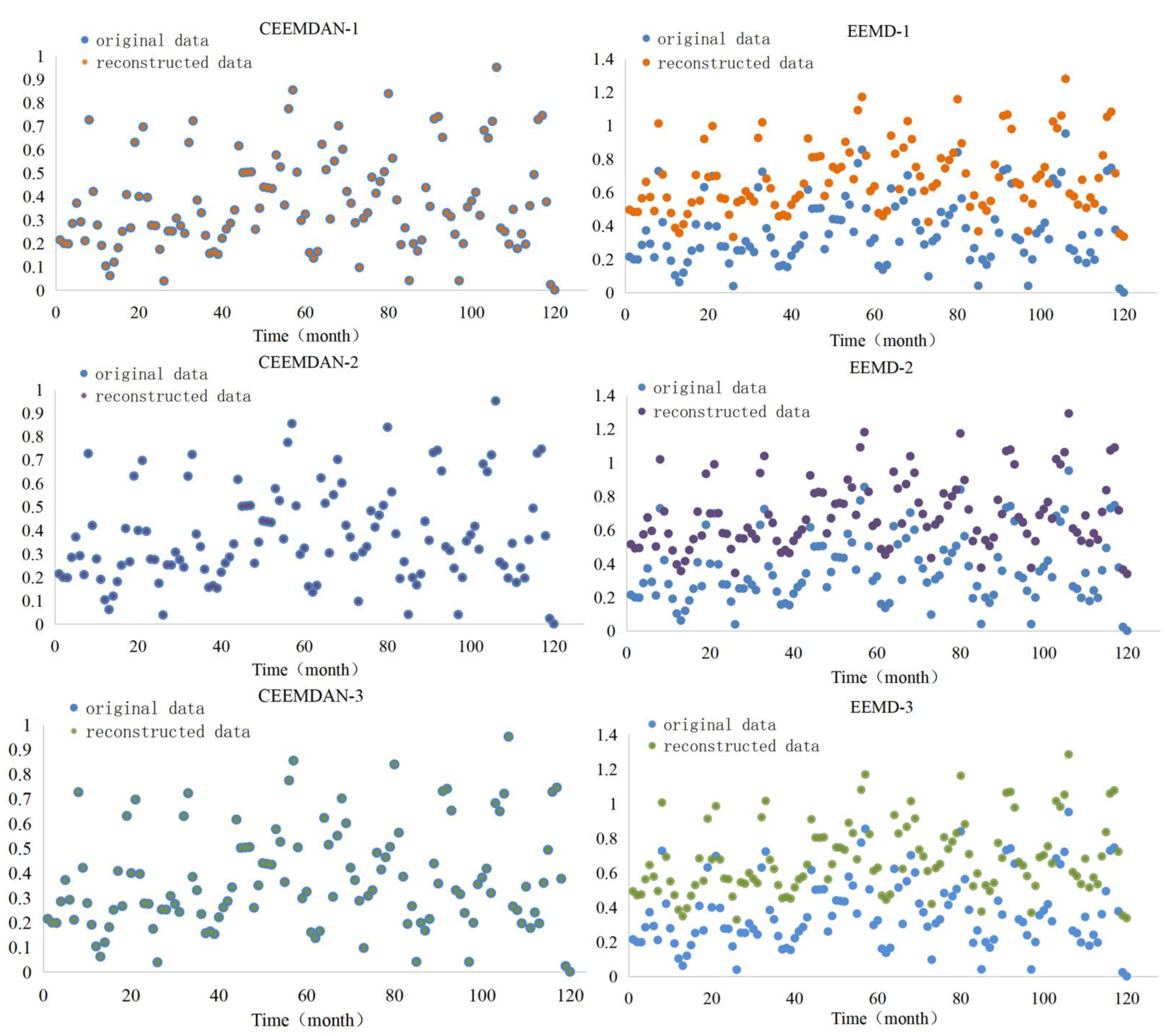
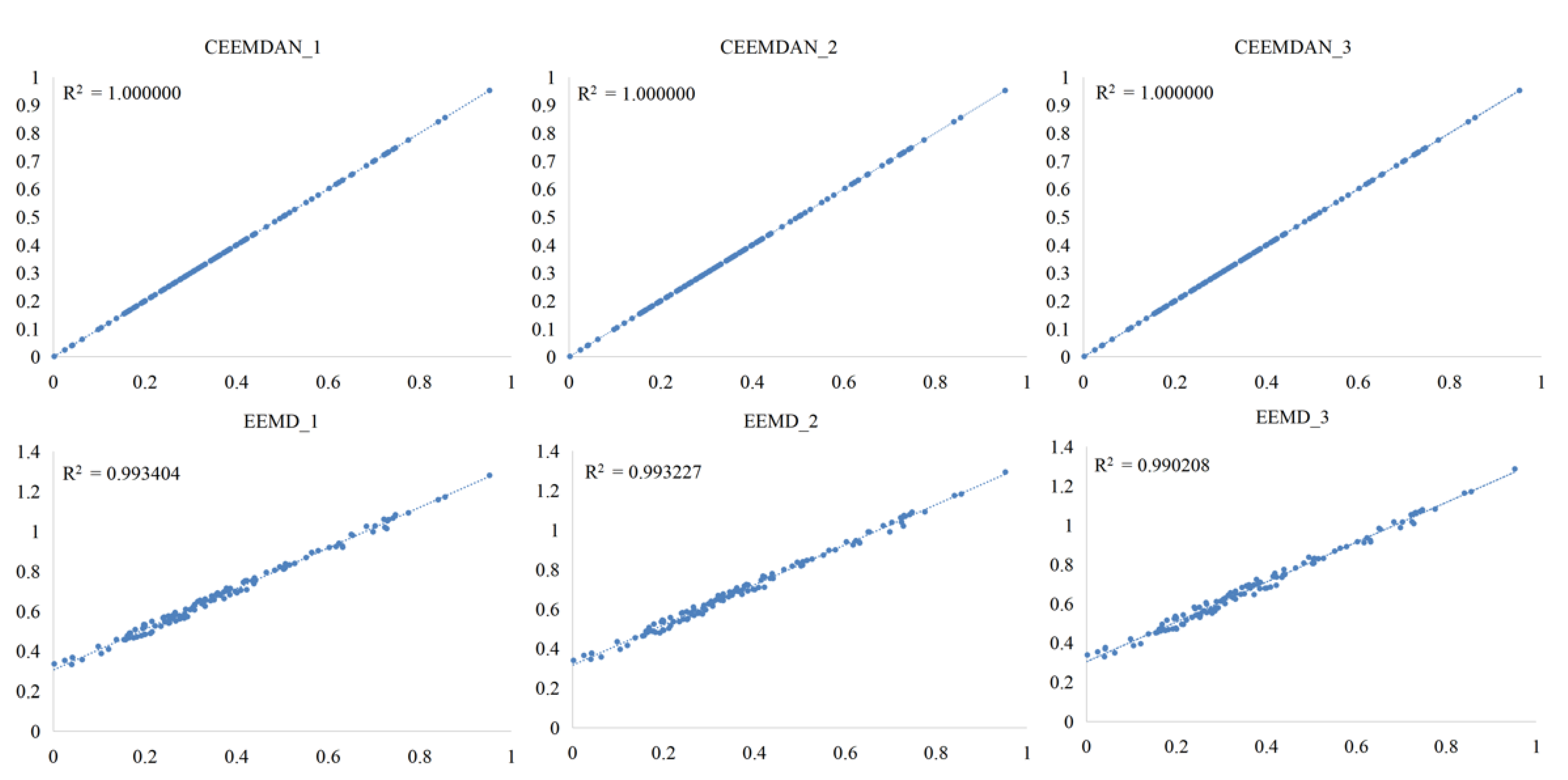
3.2. Comparison between EEMD and CEEMDAN

The EEMD and CEEMDAN algorithms were used to decompose the NDVI long time series, and the components obtained from each decomposition were reconstructed to obtain the reconstructed series based on the different decomposition algorithms. Figure 4 shows the data distribution between the original data and the reconstructed data for the three decomposition experiments based on the two algorithms. From the figure, it can be seen that the reconstructed data of CEEMDAN overlapped exactly with the original data for the three experiments, while the decomposition results of EEMD were approximately the same for each decomposition, but there was a certain deviation between the reconstructed data and the original data.

In addition, the value set data from the different reconstructed sequences of the three decomposition trials were compared with the original value set data, and the results are shown in Figure 5. For the data set used in this paper, the reconstruction accuracy of EEMD was high and reached a maximum of 99.553%, but the reconstruction accuracy of CEEMDAN was higher, and the reconstructed data fully correlated with the original data, indicating that the decomposition of CEEMDAN was able to obtain the properties of the original data by summing the components after decomposition. The reconstruction accuracy of CEEMDAN was better than that of EEMD, and the transfer of white noise from high frequency to low frequency was effectively solved in the decomposition process, which fully demonstrates the completeness of the decomposition data reconstruction of the algorithm and reflects the advantages of CEEMDAN. The CEEMDAN algorithm can better capture the transient effects of soil moisture stress that are part of the short-term stress component, which is conducive to the precise screening of soil moisture stress.

3.3. Identification of Soil Moisture Stress Components

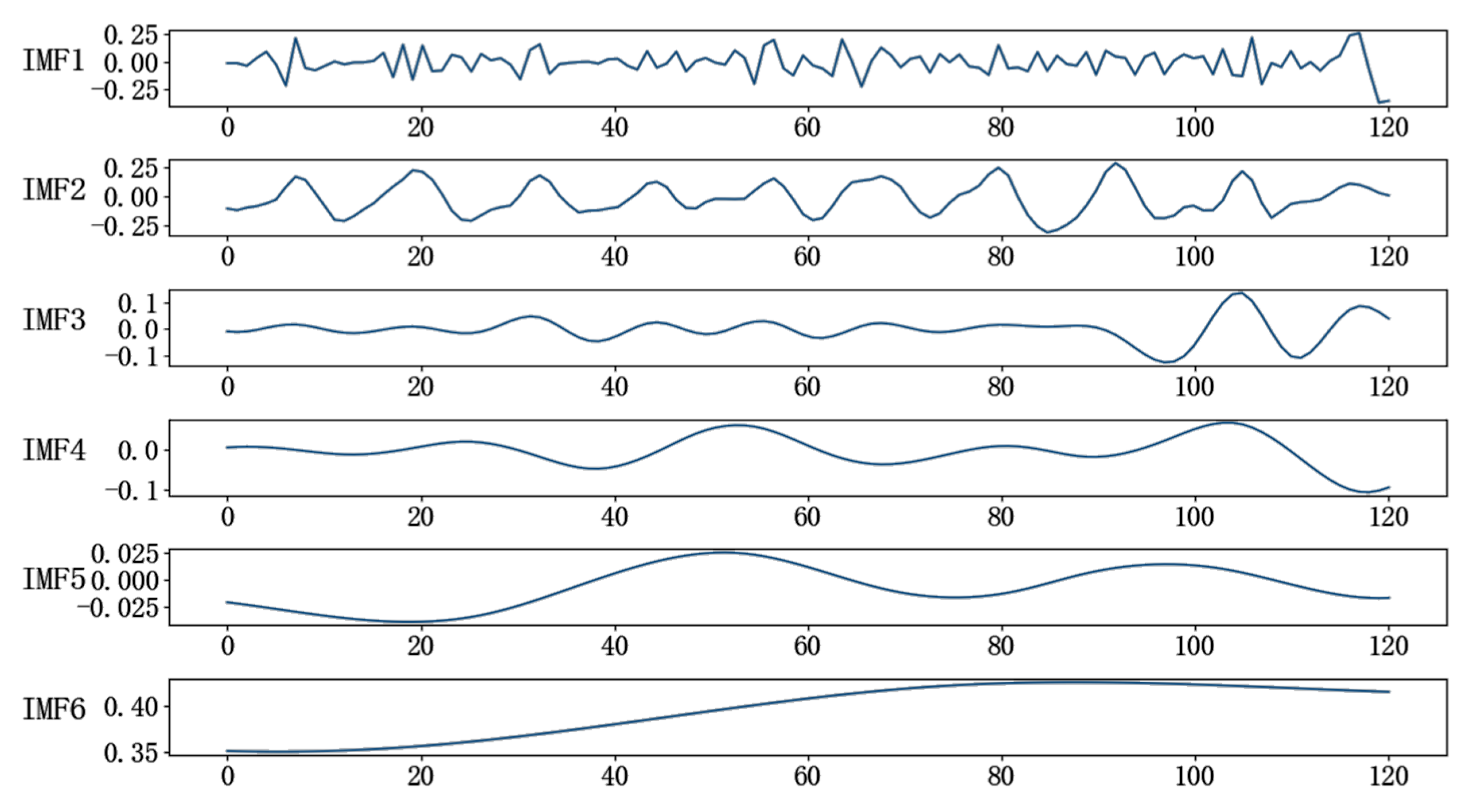
3.3.1. Decomposition Results of NDVI Long Time Series

The decomposition of the NDVI long time series was carried out based on the CEEMDAN algorithm, with the number of experiment trials set to 100 and the ext_EMD set to none. The original sequence and the six IMF components decomposed via CEEMDAN are shown in Figure 6. To compare and highlight the performance of the CEEMDAN algorithm, EEMD was also used to process the same series, and the results of EEMD are in Figure 7. As can be seen from Figure 6 and Figure 7, there was no difference in the number of decomposition components between the EEMD algorithm and the CEEMDAN algorithm; both decomposed the sequence into six IMF components. There was almost no difference in the first three IMF components, with the fluctuation frequency of the fourth component of the CEEMDAN algorithm being greater than that of the fourth component of EEMD. The difference between the two algorithms focused on the last two components, IMF₅ and IMF₆; IMF₅ and IMF₆ of the EEMD algorithm had almost the same trend, and both components fluctuated with the same amplitude, while IMF₅ and IMF₆ of the CEEMDAN algorithm had stronger independence, and the frequency and amplitude of their fluctuations were clearly distinguishable. The results of the two algorithms show that the CEEMDAN algorithm can decompose complex NDVI long time series data more effectively. It is worth noting that each component had a different frequency and amplitude of fluctuation, avoiding the problem that two components of the EEMD algorithm having the same characteristics, and that the components were more independent and better decomposed, especially in the last three low-frequency components, while the modal blending was significantly improved.

Different stress factors have certain differences in temporal and spatial characteristics. Soil heavy metals are not easily transported and are resistant to degradation, and the levels of various nutrients in soils remain in overall equilibrium within a certain range through biotic cycling in different ways. The two stresses, heavy metal stress and soil fertility stress, have relative persistence and stability. In contrast, the effects of soil moisture stress are usually more transient in time and space, occurring over one or several growth cycles, and are transient and volatile. Visual observation of the IMF components of the CEEMDAN in Figure 6 shows that the overall trend of the first two components, IMF₁ and IMF₂, was more consistent with the original data and fit the details better, with a greater frequency of fluctuations. IMF₃ and IMF₄ showed a smoother overall trend and less frequent fluctuations, while IMF₅ and IMF₆ showed a smoother trend and the least frequent fluctuations. As the number of decompositions increased, the detailed trend of the decomposed components became more blurred, the fluctuation frequency was smaller and the component curves were smoother. In conclusion, IMF₁ and IMF₂ accorded with the features of the transient and short duration of soil moisture stress better.

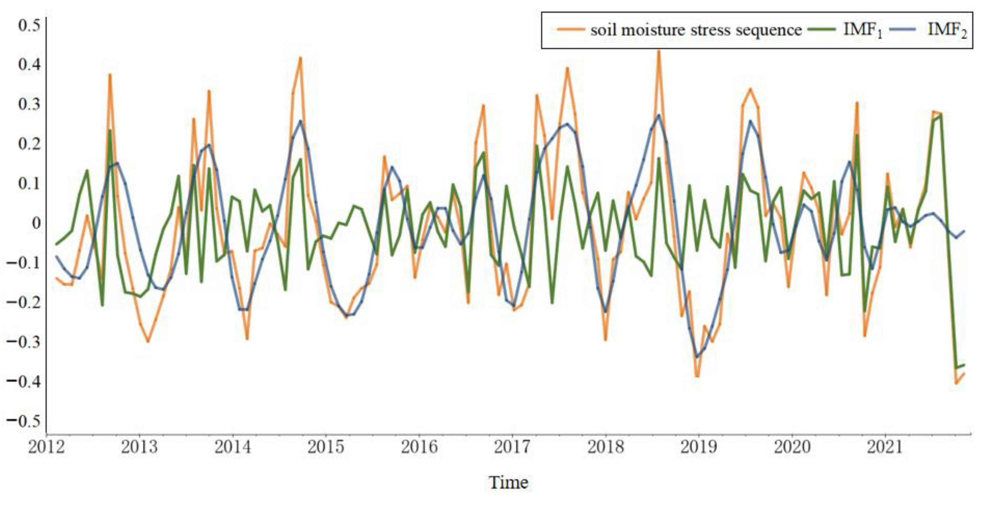
3.3.2. Identification of Soil Moisture Stress Components

To further identify the soil moisture stress subsequences scientifically and accurately, statistical descriptive indicators were calculated for each IMF, and the results are shown in

Table 2. Statistical description of IMF.

IMF	Fluctuation Period	Mean Value	Variance	Variance Contribution Rate	Pearson Correlation Coefficient
IMF1	1.600	−0.011	0.013	0.322	0.606 **
IMF2	4.286	−0.007	0.019	0.476	0.693 **
IMF3	8.000	0.002	0.007	0.160	0.304 **
IMF4	13.333	−0.001	0.002	0.042	0.133 *
IMF5	20.000	−0.003	0.001	0.011	0.197 *
IMF6	60.000	0.392	0.000	0.001	0.228 *

** Indicates a significant correlation at the 0.01 level, and * indicates a significant correlation at the 0.05 level.

. Soil moisture stress is transient and short-duration in agricultural fields and is a short-term stress, so it has a smaller fluctuation period. When a crop is stressed, the activity of chlorophyll synthase is inhibited, resulting in a lower chlorophyll content and, hence, a lower NDVI, i.e., a lower mean value at the time of stress. The variance of the data is higher when the data fluctuates widely, and the variance contribution is higher when the subsequence is more consistent with the frequency and magnitude of fluctuations in the original sequence. The shorter the duration of soil moisture stress and the smaller the fluctuation period, the greater the correlation between the component data characterizing short-term stress and the original data compared to the component data characterizing long-term stress. The fluctuation period of IMF₁ was 1.6, versus 4.285714 for IMF₂, with means of −0.010651 and −0.007224, variance contributions of 0.322034 and 0.475524, and Pearson correlation coefficients of 0.606323 and 0.693123. IMF₄, IMF₅ and IMF₆ all had relatively large fluctuation periods with scales larger than the interannual scale, while IMF₃ had a relatively small fluctuation period and mean, but IMF₃ had a small variance, variance contribution and Pearson correlation coefficient. According to the above analysis, IMF₁ and IMF₂ were identified as soil moisture stress subsequences. The soil moisture stress sequence in Figure 8 was obtained via the cumulative synthesis of the two according to the following equation, which characterized the effect of soil moisture stress of winter wheat.

$$y(t)={\displaystyle \sum _{t=1}^T({\mathrm{IMF}}_1(t)+{\mathrm{IMF}}_2(t))}$$

(12)

The synthesis of the soil moisture stress sequence combined the effects of the two soil moisture stress characteristic components of IMF₁ and IMF₂, covering the characteristic information of both the IMF₁ and IMF₂ subsequences. For the IMF₁ and IMF₂ subsequence in Figure 8, the IMF₁ subsequence had a smaller fluctuation period and a higher fluctuation frequency, but its variance and variance contribution were smaller, and its upward and downward fluctuations were relatively small. The IMF₂ subsequence had a smaller fluctuation period and a slower fluctuation frequency than IMF₁, but its variance and variance contribution were larger, and its upward and downward fluctuations were relatively large. The mean values of IMF₁ and IMF₂ were similar, with both curves fluctuating around the zero value line, and the mean values of the synthetic soil moisture stress sequences were also similar to the mean values of the two subseries. The fluctuation period of the soil moisture stress sequence neutralized the fluctuation periods of the two subsequences, IMF₁ and IMF₂, but the fluctuations were larger compared to the two subsequence curves. The lower the amount of soil moisture stress compared to normal, the deeper the soil moisture stress.

3.4. Soil Moisture Stress Response Index

The soil moisture stress sequence was non-smooth and non-linear in the long time scale, but it showed certain regular characteristics in a short time. SMSC was obtained via fitting the soil moisture stress characteristic curve with the measured data; part of the measured data is shown in

Table 3. Partial list of the measured data.

Stage	Relative Chlorophyll Content (SPAD)	PMC (%)	SMC (%)
Jointing stage	54.3	78.1	11.2
	48.4	81.7	11.5
	54.0	82.6	14.8
	47.9	81.2	9.9
Booting stage	47.5	82.4	9.5
	49.3	79.0	11.4
	45.3	76.5	9.3
	46.5	80.8	10.8
Heading stage	50.3	82.3	10.5
	49.5	76.5	10.6
	52.1	76.3	9.6
	54.8	80.3	14.1
Flowering stage	50.4	69.4	9.6
	62.0	76.9	13.4
	59.1	73.9	10.6
	56.5	77.1	12.3
Filing stage	52.6	71.5	11.7
	66.9	71.3	9.2
	62.9	70.4	10.1
	57.4	69.6	11.0

.

The chlorophyll content remained stable at the jointing, booting and heading stages, with a small increase in chlorophyll content as the leaves grew more densely at the flowering and filling stages. The plant moisture content remained stable at the jointing, booting and heading stages, with a small decrease at the flowering and filling stages as the dry matter mass of the winter wheat plant increased. The soil moisture content varied from one sampling point to another due to factors such as topography and hydrological conditions, and it also varied from one fertility period to another with the passage of time, precipitation, irrigation and other factors. CR_SMS indicates the response characteristics of chlorophyll to soil moisture stress, and WMCR_SMS indicates the response characteristics of wheat moisture content to soil moisture stress. Various model types, such as quadratic, cubic, composite and growth, were used, and the results show that the quadratic, cubic and growth models had higher R² and better results. Among them, the cubic model is the best fit for both indicators. This means that the fitting results are representative and stable, and the two indices CR_SMS and WMCR_SMS can effectively reflect the response to soil moisture stress.

3.5. Construction and Validation of the Inversion Model

In this study, the three indicators SMSC, CR_SMS and WMCR_SMS were used as independent variables, and the SMC was used as a dependent variable of the PLSR model to construct the inversion model. In CEEMDAN, the parameter epsilon is the proportion of noise added, which affects the decomposition results and, furthermore, the final inversion accuracy. In this paper, we took epsilon as 0.005, 0.01, 0.05, 0.1, 0.2 and 0.3, and the long time series were decomposed several times according to the experimental procedure.

After several trials, the results are shown in Figure 9. When epsilon was in the 0.005 to 0.05 range, the R² of the constructed model generally tended to increase, and the corresponding MAE and RMSE generally tended to decrease. When epsilon was 0.005 and 0.01, the accuracy of the model was comparable, and there was almost no difference between the three evaluation indicators, and compared with the other values, the R² of the model was lower, MAE and RMSE were higher and the overall accuracy of the model was lower. When epsilon was 0.05 to 0.3, the R² of the model decreased, and the MAE and RMSE increased. When epsilon was 0.05, the R² of the model reached a maximum of 0.963, the corresponding MAE and RMSE were the lowest, at 0.068 and 0.250, respectively, and the decomposition effect was optimal.

Based on the results of the previous experiment, we set the decomposition parameter epsilon to 0.05 and constructed PLSR inversion models with three types of linear, quadratic and cubic polynomials. The experiment was set up with three replications, and R², MAE and RMSE were finally calculated for each model (

Table 4. Comparison of the model accuracy evaluation results.

Algorithm	Number of Tests	Model Type	Model Accuracy Evaluation Index
			R2	MAE	RMSE	p-Value
CEEMDAN	1	Linear	0.841	0.141	0.336	8.14 × 10−3
		Quadratic	0.931	0.093	0.288	4.85 × 10−3
		Cubic	0.874	0.125	0.320	7.36 × 10−3
	2	Linear	0.903	0.110	0.314	5.62 × 10−3
		Quadratic	0.981	0.048	0.202	9.75 × 10−4
		Cubic	0.960	0.070	0.236	3.51 × 10−3
	3	Linear	0.900	0.112	0.315	5.74 × 10−3
		Quadratic	0.979	0.051	0.210	9.83 × 10−4
		Cubic	0.957	0.073	0.239	4.07 × 10−3

).

The results of several tests showed that the Quadratic PLSR inversion model gave the best results among the three models, with the second test model having the highest R² of 0.981, as well as the lowest MAE and RMSE of 0.048 and 0.202. And the relative error of the model was the smallest, at 7.926%. In any case, the optimal inversion model was obtained when epsilon was 0.05 and the model type was quadratic. The results of the accuracy evaluation demonstrated that the optimal model improved in various indicators compared with previous inversion models. The specific inversion model and indicators are shown in

Table 5. Inversion model of multi-indicators based on PLSR.

Model Type	Regression Equation	R2	MAE	RMSE	Error (%)
Linear	$\mathrm{SMC}=12.738-0.042x_1+0.022x_2-8.905x_3$	0.903	0.110	0.314	11.203
Quadratic	$\begin{array}{cc}\mathrm{SMC}=& 20.58-0.02x_1+0.01x_2-1.76x_3-\\ & 2\times {10}^{-3}{x}_1{x}_2-0.065x_1{x}_3-0.045x_2{x}_3-\\ & 1.83\times {10}^{-4}{x}_1{}^2+7.91\times {10}^{-5}{x}_2{}^2+3.99x_3{}^2\end{array}$	0.981	0.048	0.202	7.926
Cubic	$\begin{array}{cc}\mathrm{SMC}=& 16.66-9\times {10}^{-3}{x}_1+5\times {10}^{-3}{x}_2-0.527x_3-\\ & 8.8\times {10}^{-4}{x}_1{x}_2-0.02x_1{x}_3-0.014x_2{x}_3-\\ & 7.8\times {10}^{-5}{x}_1{}^2-3.4\times {10}^{-5}{x}_2{}^2-2.33x_3{}^2+\\ & 18.55x_3{}^3-7.5\times {10}^{-4}{x}_1{x}_2{x}_3-5.4\times {10}^{-4}{x}_1{}^2{x}_3-\\ & 0.14x_1{x}_3{}^2-2.6\times {10}^{-4}{x}_2{}^2{x}_3-0.086x_2{x}_3{}^2\end{array}$	0.960	0.070	0.236	8.518

.

In the regression models of Table 5, $x_1$ represents CR_SMS, $x_2$ represents WMCR_SMS and $x_3$ represents for SMSC. The $x_1{}^2{x}_2$, $x_1{x}_2{}^2$, $x_1{}^3$ and $x_2{}^3$ terms in the cubic type model had coefficients below 1 × 10⁻⁵, so they were excluded from the regression model equation.

3.6. Spatial and Temporal Distribution of Soil Moisture Content

The CEEMDAN algorithm was used to decompose the NDVI long time series of winter wheat to obtain the soil water stress in February, March, April and May at each sampling site and then calculate the chlorophyll response and plant water response to soil water stress based on the fitting results. The inversion model was used to invert the soil water content for February, March, April and May at each sampling site. The inverse soil water content was assigned to the attribute column of the sampling point vector, and the results were interpolated using the inverse distance weighted interpolation (IDW) method in the Spatial Analysis Tools module of ArcGIS 10.2 to obtain an interpolation map based on the soil water content attribute column. The interpolation results were then extracted using the Mask Extraction tool in the Extraction Analysis module to analyze the spatial and temporal distribution and trends of soil water content via farmland support vector machine classification. The spatial distribution of soil water content at the monthly scale for February, March, April and May was obtained as shown in Figure 10. The redder the color, the lower the soil water content and the more affected by soil moisture stress, and the bluer the color, the higher the soil water content and the less affected by soil moisture stress.

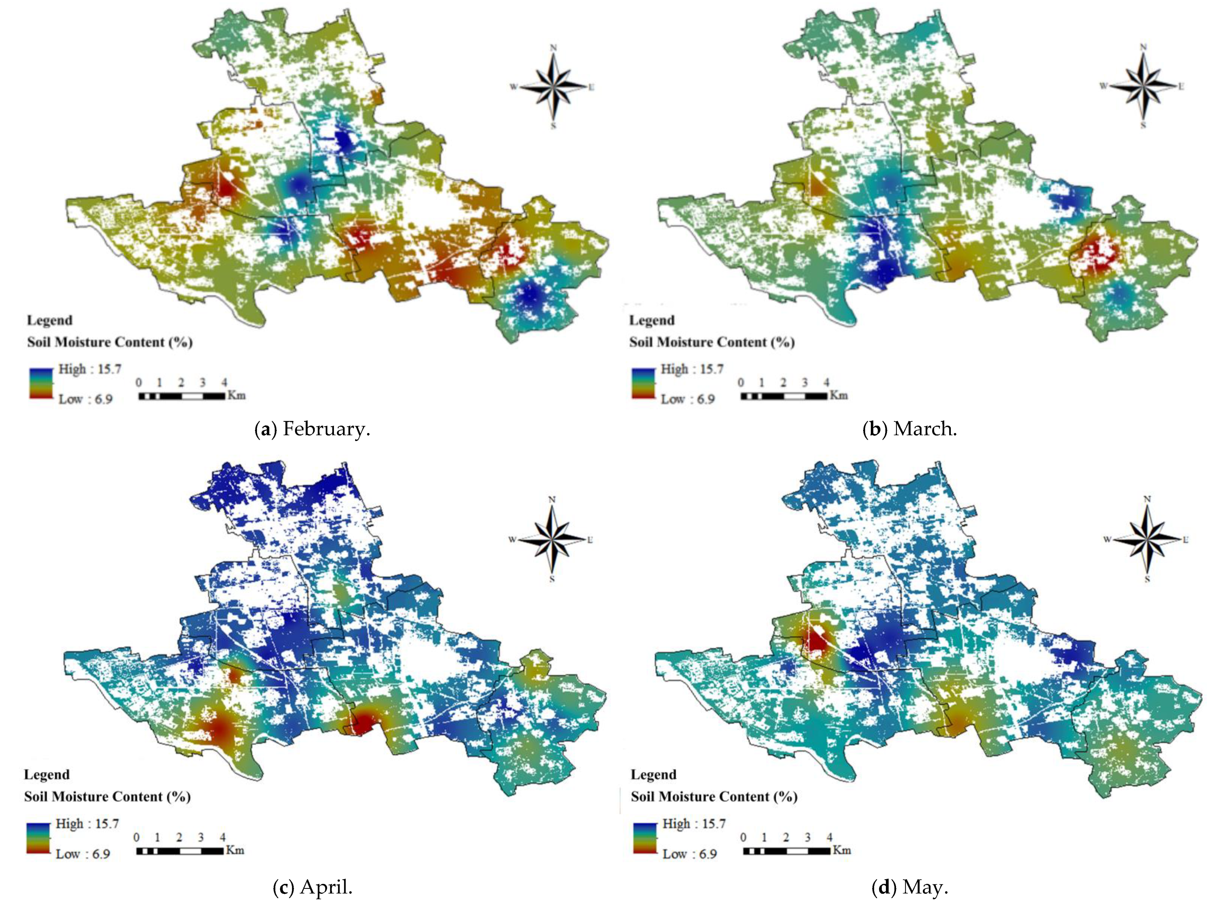
3.6.1. Spatial Distribution Characteristics of Soil Moisture Content

The soil moisture content of farmland in the study area was generally in the range of 6.9% to 15.7%. According to relevant information, when the soil moisture content is 18.5% to 20%, it is a state of full moisture, which is the upper limit of the suitable tillage for farmland, and the effective soil moisture content is the highest. When the soil moisture content is 15.5% to 18.5%, it is a suitable moisture condition for farmland sowing and cultivation, and the effective moisture content is high. When the soil moisture content is 12% to 15%, it is yellow moisture, which is suitable for cultivation, but the effective moisture content is low, and the seedlings are not sown in unison and need irrigation. When the soil moisture content is below 8%, the soil is dry, and there is no water for crops to absorb, making it unsuitable for cultivation and sowing. The vast majority of the fields in the study area were basically in a yellow moisture state and needed to be irrigated during the growth of winter wheat.

The optimal inversion model was used to invert the soil moisture content over a large area of farmland in the whole study area (Figure 10) to provide a reference basis for irrigation. The soil moisture content of the farmland in the study area was basically in the range of 6.9% to 15.7%, which is suitable for farming, but the effective water content was low, and it was difficult to meet the growth demand of wheat with soil moisture alone, so irrigation was required. The spatial distribution indicated that the soil moisture content was low in the central part, and stress conditions were more prominent in the central and southern parts, mainly including the southern part of Xiadian, the northern part of Shaofu, the western part of Dachang, the area around Fenglanzhuang in Qigezhuang and the northernmost part of Chenfu. In the northern part of the study area, namely the northern part of Xiadian, this part of the terrain is higher, and the water table is deeper, making it more prone to droughts than to floods. The soils in the southwest and southeast have high water content, especially in the southeast. The southwestern part has a sandy, loamy, tidal brown soil with a sandy texture and strong water leakage and aeration, but the southwestern town of Qigezhuang is close to the Chaobai River; this part of the town has good conditions for well and canal irrigation, and the soil moisture content of the agricultural land is medium to high. The Wangbitun, Liangzhuang and Yuanzhuang villages in Dachang and the middle and southern part of Chenfu, as well as the southeastern part of Shaofu and the eastern part of Qigezhuang, are tidal soil areas, which are low-lying and have the highest soil moisture content. In summary, the southeastern part of the study area, the southeastern part of Shaofu and the eastern part of Qigezhuang are less stressed by soil moisture and have a higher soil moisture content. The central part of the study area, especially the south-central part, is the most stressed by soil moisture and has the lowest soil moisture content, and winter wheat growing areas should pay extra attention to irrigation in spring, the reasonable use of well irrigation, canal irrigation and other irrigation conditions to meet the water needs of wheat growth.

3.6.2. Temporal Distribution Characteristics of Soil Moisture Content

Through the overall observation of Figure 10, it was found that the soil moisture content showed an overall increasing trend from February to May, with April and May having relatively high soil moisture content and February and March having low soil moisture content. Figure 10a shows the distribution of soil moisture content in February, from which it can be seen that the overall study area is greatly affected by soil moisture stress and has the lowest soil moisture content, with some areas appearing in red. The distribution of soil moisture content in March is shown in Figure 10b, where the red areas are larger, the soil moisture content is lower and the drought is more severe than in the other months, and the growth of winter wheat is most vulnerable to soil moisture stress. The soil moisture content in April is shown in Figure 10c. Compared with March, the overall soil moisture content has increased, with the overall red color lighter than in the previous two months, with the northern part of Chenfu town and the northeastern part of Qigezhuang being darker in red and most of the other areas being affected by soil moisture stress to some extent but not to a great extent. Figure 10d shows the distribution of soil moisture content in May, with most areas being yellow–green and blue, except for the southernmost part of Dachang town and the northernmost part of Qigezhuang town, which are less affected by soil moisture stress at this time.

In combination with the above analysis, February is a low-temperature month, and winter wheat has just passed the overwintering period; it does not require much water. March has lower soil moisture content and is more affected by soil moisture stress, and early March to mid-April contains the crucial greening, rising and jointing period for winter wheat, so it needs to be watered in time to replenish soil moisture. The average temperature in March is low, and irrigation at this time is likely to cause frost damage to wheat, so the spring irrigation of winter wheat occurs mainly during the jointing period in April. The period from late April to late May contains important periods such as the booting, heading and flowering stages, and the soil moisture stress level directly affects the yield of winter wheat, which requires more water. The soil moisture content in most areas of the study area was close to 15% in May, but with the increase in temperature, the evaporation of water from the soil surface layer increased, and the monitoring of soil moisture content in the central part of the study area, especially in the south-central part, needs to be strengthened in May. In conclusion, from February to May, the degree of soil moisture stress in winter wheat gradually decreases with time, and in spring, February and March are the months with low soil moisture content, and attention should be paid to the management of spring irrigation, the timely replenishment of farm moisture and the appropriate strengthening of real-time soil moisture monitoring.

4. Discussion

In this study, we used CEEMDAN to decompose the NDVI long time series to screen soil moisture stress, and we constructed a soil moisture content inversion model based on PLSR, providing a new way to accurately monitor and accurately invert soil moisture content. In studies of soil moisture stress and soil moisture content based on remote sensing technology, the inversion of soil moisture content has involved uncertainty, but the long time series we constructed conformed to the characteristics of the sawtooth bimodal time series curve under the biannual cropping system in the study area. The R² of the soil moisture content inversion model based on CEEMDAN–PLSR reached 98.1%, and the relative error for model accuracy verification was 7.9%; this suggests the value and significance of our study of soil moisture content inversion based on the long time series and CEEMDAN. The optimal parameters and inversion type were determined through several tests of the CEEMDAN decomposition parameters and the PLSR model construction type, and the optimal inversion model obtained based on these results can effectively invert the soil moisture content over a large area. In the practical application of the optimal model, the spatial and temporal distribution characteristics of the soil moisture content of agricultural land were analyzed in conjunction with the inversion results, and the analytical features were consistent with the characteristics of the topography and soil properties of the study area.

Soil moisture stress has the characteristics of short-term and transient sudden changes, some studies have realized the extraction of long-term stress factors from the EEMD decomposition results [35,36,37], and the screening of long-term stress factors can also assist in further realizing the extraction of short-term stress factors. The high performance of the CEEMDAN algorithm is the basis for the accurate decomposition and screening extraction of the characteristic components of soil moisture stress. Previous studies have found that NDVI is more sensitive to vegetation in semi-arid regions, indicating that NDVI may provide a better estimate of soil moisture in the root zone of semi-arid regions. It is important to recognize that NDVI has good sensitivity to soil moisture and precipitation. In this study, we found that the retrieved soil moisture content shown in Figure 10 was in the range of 6.9–15.7%, belonging to a lower level, which may be due to three reasons. Firstly, Dachang Hui Autonomous County in Langfang, Hebei Province, belongs to a warm-temperate, semi-humid continental monsoon climate, which is usually accompanied by significant seasonal precipitation changes. During the dry season from February to May, there is less precipitation and a decrease in soil moisture. According to the measured soil moisture values in the field from March to June 2023, the average soil moisture in the five regions ranged from 0.11 to 0.15. The actual measurement results indicate that, under normal conditions during the dry season in the study area, the range of soil surface moisture content is indeed at a relatively low level. Secondly, during the dry season from February to May in Dachang Hui Autonomous County, the precipitation situation is shown in Figure 11. We used the precipitation data from Suzhou Baoshan Meteorological Station in southeastern China for comparison. Especially during the spring and dry seasons, the daily average precipitation in the Dachang area is minimal or even non-existent. The figure indicates that sunny days are the main weather for spring droughts in the study area. And on days when we visualized the spatial distribution of surface moisture and soil moisture (25 February, 26 March, 16 April and 26 May 2023), there was also no natural precipitation. If there is natural precipitation, the soil moisture retrieved after a rainy day may be higher, exceeding 15.7% or even higher. Finally, it should be pointed out that the field measurements did not consider collecting soil moisture values on rainy days or irrigation conditions, and the collected samples were also in non-irrigation areas or on non-irrigation dates. The results show that the inversion obtained using the model is basically consistent with the measured values in the non-irrigated areas of Dachang Hui Autonomous County under normal conditions. This study provides a reliable spatiotemporal distribution of soil moisture content for the dry season in monsoon climate zones, which shows great potential in preventing agricultural drought and taking timely irrigation measures.

The use of optical remote sensing and microwave remote sensing for inversion has its own advantages and disadvantages, and the integrated use of optical and microwave remote sensing to achieve the accurate inversion of soil moisture content and further improve the accuracy of inversion is an important research direction for the future. Also, the PLSR multi-indicator inversion model can incorporate measured soil moisture data after just rainfall or irrigation to evaluate the ability of the CEEMDAN algorithm to extract short-term stress factors and quantitatively study the impact of natural precipitation or artificial irrigation on the transient changes in soil moisture.

5. Conclusions

In this study, the NDVI long time series in a natural farmland ecosystem was constructed based on remote sensing data, CEEMDAN decomposition was performed to obtain each IMF component and five statistical descriptive indexes of each IMF component were calculated and compared with each other. Soil moisture stress subsequences were extracted and synthesized to obtain a soil moisture stress sequence. PLSR was used to establish an inversion model, and comparison tests were conducted to select the optimal inversion model to finally realize the precise monitoring and quantitative inversion of soil moisture content. Based on the optimal model, the spatio- and temporal distribution characteristics of soil moisture content were analyzed:

(1)

The CEEMDAN algorithm decomposes the data with higher reconstruction accuracy, reduces the interference of noise on NDVI long time series and preserves the details of the data. It excludes the impact of other noise stress factors, which facilitates the accurate screening of soil moisture stress and improves the accuracy of soil moisture content inversion;

(2)

Two response indices can exactly present the response of chlorophyll content and wheat moisture content to soil moisture stress. The CEEMDAN algorithm gives the best decomposition when the ratio of added noise is set to 0.05. Meanwhile, when the inversion model type is a quadratic model, the model determination coefficient R² reaches a maximum of 0.981, with a high degree of model fit and low error, and the Qudratic CEEMDAN–PLSR inversion model has high inversion accuracy and stability;

(3)

The effective soil moisture content in the study area is relatively low. The degree of soil moisture stress gradually decreases from February to May, and attention should be paid to the management of spring irrigation in April, the timely replenishment of farm moisture and the appropriate strengthening of real-time soil moisture monitoring to the central part, especially the south-central part.

This means that the combination of time–frequency analysis technology and remote sensing technology can achieve the real-time and accurate monitoring of soil moisture over a large area, providing a basis for decision-making in agricultural irrigation and contributing to the rational use of water resources and the sustainable development of the agricultural economy. However, there are still limitations and room for improvement in the study. Firstly, the use of optical and microwave remote sensing for inversion has its own advantages and disadvantages, and the integrated use of the two to achieve the accurate inversion of soil moisture content is an important research direction. Secondly, the number of ground data measurements in this study was relatively small, and the actual collection of parameter indicators on the ground and the amount of data were limited by the epidemic and other reasons. In future research, we can increase the dimensionality of the parameters, expand the amount of data to fit with the remote sensing monitoring data and seek a better inversion model of soil moisture content from multiple scales.

References

1. Zhao, J.; Zhang, C.; Min, L.; Guo, Z.; Li, N. Retrieval of Farmland Surface Soil Moisture Based on Feature Optimization and Machine Learning. Remote Sens. 2022, 14, 5102. [Google Scholar] [CrossRef]
2. Zhang, Y.; Liu, X.; Jiao, W.; Zeng, X.; Xing, X.; Zhang, L.; Yan, J.; Hong, Y. Drought monitoring based on a new combined remote sensing index across the transitional area between humid and arid regions in China. Atmos. Res. 2021, 264, 105850. [Google Scholar] [CrossRef]
3. Mirzaei, A.; Naseri, R.; Moghadam, A.; Esmailpour-Jahromi, M. The effects of drought stress on seed yield and some agronomic traits of canola cultivars at different growth stages. Bull. Environ. Pharmacol. Life Sci. 2013, 2, 115–121. [Google Scholar]
4. Kapoor, D.; Bhardwaj, S.; Landi, M.; Sharma, A.; Ramakrishnan, M.; Sharma, A. The Impact of Drought in plant metabolism: How to exploit tolerance mechanisms to increase crop production. Appl. Sci. 2020, 10, 5692. [Google Scholar] [CrossRef]
5. Huang, S.; Huang, Q.; Chang, J.; Leng, J.; Xing, L. The response of agricultural drought to meteorological drought and the influencing factors: A case study in the Wei River Basin, China. Agric. Water Manag. 2015, 159, 45–54. [Google Scholar] [CrossRef]
6. Wu, X.; Bai, M.; Li, Y.; Du, T.; Zhang, S.; Shi, Y. Effect of water and fertilizer coupling on root growth, soil water and nitrogen distribution of cabbage with drip irrigation under mulch. Trans. Chin. Soc. Agric. Eng. 2019, 35, 110–119. [Google Scholar]
7. Liu, M.; Liu, X.; Zhang, B.; Ding, C. Regional heavy metal pollution in crops by integrating physiological function variability with spatio-temporal stability using multi-temporal thermal remote sensing. Int. J. Appl. Earth Obs. Geoinf. 2016, 51, 91–102. [Google Scholar] [CrossRef]
8. Liu, M.; Wang, T.; Skidmore, A.; Liu, X. Heavy metal-induced stress in rice crops detected using multi-temporal Sentinel-2 satellite images. Sci. Total Environ. 2018, 637–638, 18–29. [Google Scholar] [CrossRef]
9. Cui, T.; Zhang, Z.; Cui, C.; Bian, J.; Chen, S.; Wang, H. Study on Variation Curve and Fitting Model of Winter Wheat Canopy NDVI. Water Sav. Irrig. 2018, 12, 97–103. [Google Scholar]
10. Wang, Q.; Li, M.; Li, G.; Zhang, J.; Yan, S.; Chen, Z.; Zhang, X.; Chen, G. High-Resolution Remote Sensing Image Change Detection Method Based on Improved Siamese U-Net. Remote Sens. 2023, 15, 3517. [Google Scholar] [CrossRef]
11. Wang, R.; Zhao, J.; Yang, H.; Li, N. Inversion of Soil Moisture on Farmland Areas Based on SSA-CNN Using Multi-Source Remote Sensing Data. Remote Sens. 2023, 15, 2515. [Google Scholar] [CrossRef]
12. Milewski, R.; Schmid, T.; Chabrillat, S.; Jiménez, M.; Escribano, P.; Pelayo, M.; Ben-Dor, E. Analyses of the Impact of Soil Conditions and Soil Degradation on Vegetation Vitality and Crop Productivity Based on Airborne Hyperspectral VNIR–SWIR–TIR Data in a Semi-Arid Rainfed Agricultural Area (Camarena, Central Spain). Remote Sens. 2022, 14, 5131. [Google Scholar] [CrossRef]
13. Albertini, C.; Gioia, A.; Iacobellis, V.; Manfreda, S. Detection of Surface Water and Floods with Multispectral Satellites. Remote Sens. 2022, 14, 6005. [Google Scholar] [CrossRef]
14. Liu, S.; Tian, W.; Yin, Y.; An, N.; Dong, S. Temporal dynamics of vegetation NDVI and its response to drought conditions in Yunnan Province. Acta Ecol. Sin. 2016, 36, 4699–4707. [Google Scholar]
15. Celik, M.F.; Isik, M.S.; Yuzugullu, O.; Fajraoui, N.; Erten, E. Soil Moisture Prediction from Remote Sensing Images Coupled with Climate, Soil Texture and Topography via Deep Learning. Remote Sens. 2022, 14, 5584. [Google Scholar] [CrossRef]
16. Liu, W.; Zhu, S.; Huang, Y.; Wan, Y.; Wu, B.; Liu, L. Spatiotemporal Variations of Drought and Their Teleconnections with Large-Scale Climate Indices over the Poyang Lake Basin, China. Sustainability 2020, 12, 3526. [Google Scholar] [CrossRef]
17. Hirschberg, V.; Rodrigue, D. Fourier Transform (FT) Analysis of the Stress as a Tool to Follow the Fatigue Behavior of Metals. Appl. Sci. 2021, 11, 8. [Google Scholar] [CrossRef]
18. Hien, L.T.T.; Gobin, A.; Lim, D.T.; Quan, D.T.; Hue, N.T.; Thang, N.N.; Binh, N.T.; Dung, V.T.K.; Linh, P.H. Soil Moisture Influence on the FTIR Spectrum of Salt-Affected Soils. Remote Sens. 2022, 14, 2380. [Google Scholar] [CrossRef]
19. Zhang, M.; Zhou, Q.; Chen, Z.; Jia, L.; Zhou, Y.; Cai, C. Crop discrimination in Northern China with double cropping systems using Fourier analysis of time-series MODIS data. Int. J. Appl. Earth Obs. Geoinf. 2008, 10, 476–485. [Google Scholar]
20. Lokeshwara, R.; Pawar, S.; Prathapa, R. Curvelet Transform based Denoising of Multispectral Remote Sensing Images. J. Phys. Conf. Ser. 2021, 1, 2089. [Google Scholar] [CrossRef]
21. Wongsaroj, W.; Hamdani, A.; Thong-Un, N.; Takahashi, H.; Kikura, H. Extended Short-Time Fourier Transform for Ultrasonic Velocity Profiler on Two-Phase Bubbly Flow Using a Single Resonant Frequency. Appl. Sci. 2018, 9, 50. [Google Scholar] [CrossRef]
22. Yang, C.; Liu, P.; Yin, G.; Jiang, H.; Li, X. Defect detection in magnetic tile images based on stationary wavelet transform. NDT E Int. 2016, 83, 78–87. [Google Scholar] [CrossRef]
23. Feng, X.; Zhang, W.; Su, X.; Xu, Z. Optical Remote Sensing Image Denoising and Super-Resolution Reconstructing Using Optimized Generative Network in Wavelet Transform Domain. Remote Sens. 2021, 13, 1858. [Google Scholar] [CrossRef]
24. Ebrahimi, K.; Taghizadeh, M.; Kazemi, M.; Nafarzadegan, R. Predicting the ground-level pollutants concentrations and identifying the influencing factors using machine learning, wavelet transformation, and remote sensing techniques. Atmos. Pollut. Res. 2021, 12, 5. [Google Scholar] [CrossRef]
25. Hu, Z.; Chai, L.; Crow, W.T.; Liu, S.; Zhu, Z.; Zhou, J.; Qu, Y.; Liu, J.; Yang, S.; Lu, Z. Applying a Wavelet Transform Technique to Optimize General Fitting Models for SM Analysis: A Case Study in Downscaling over the Qinghai–Tibet Plateau. Remote Sens. 2022, 14, 3063. [Google Scholar] [CrossRef]
26. Liu, Z.; Zhao, L.; Peng, Y.; Wang, G.; Hu, Y. Improving Estimation of Soil Moisture Content Using a Modified Soil Thermal Inertia Model. Remote Sens. 2020, 12, 1719. [Google Scholar] [CrossRef]
27. Li, D.; Che, X.; Luo, W.; Hu, Y.; Wang, Y.; Yu, Z.; Yuan, L. Digital watermarking scheme for colour remote sensing image based on quaternion wavelet transform and tensor decomposition. Math. Methods Appl. Sci. 2019, 42, 4664–4678. [Google Scholar] [CrossRef]
28. Zhang, C.; Liu, J.; Su, W.; Qiao, M.; Zhu, D. Optimal scale of crop classification using unmanned aerial vehicle remote sensing imagery based on wavelet packet transform. Editor. Off. Trans. Chin. Soc. Agric. Eng. 2016, 32, 95–101. [Google Scholar]
29. Masoud, M. Wavelet transform approach for denoising and decomposition of satellite-derived ocean color time-series: Selection of optimal mother wavelet. Adv. Space Res. 2022, 69, 2724–2744. [Google Scholar]
30. Wang, C.; Sun, W.; Fan, D.; Liu, X.; Zhang, Z. Adaptive Feature Weighted Fusion Nested U-Net with Discrete Wavelet Transform for Change Detection of High-Resolution Remote Sensing Images. Remote Sens. 2021, 13, 4971. [Google Scholar] [CrossRef]
31. Nassar, A.; Torres-Rua, A.; Hipps, L.; Kustas, W.; McKee, M.; Stevens, D.; Nieto, H.; Keller, D.; Gowing, I.; Coopmans, C. Using Remote Sensing to Estimate Scales of Spatial Heterogeneity to Analyze Evapotranspiration Modeling in a Natural Ecosystem. Remote Sens. 2022, 14, 372. [Google Scholar] [CrossRef]
32. Asim, B. Scale–location specific soil spatial variability: A comparison of continuous wavelet transform and Hilbert–Huang transform. Catena 2018, 160, 24–31. [Google Scholar]
33. Wang, X.; Liu, A.; Zhang, Y.; Xue, F. Underwater Acoustic Target Recognition: A Combination of Multi-Dimensional Fusion Features and Modified Deep Neural Network. Remote Sens. 2019, 11, 1888. [Google Scholar] [CrossRef]
34. Fu, P.; Zhang, W.; Yang, K.; Meng, F. A novel spectral analysis method for distinguishing heavy metal stress of maize due to copper and lead: RDA and EMD-PSD. Ecotoxicol. Environ. Saf. 2020, 206, 111211. [Google Scholar] [CrossRef]
35. Prasad, R. Streamflow and soil moisture forecasting with hybrid data intelligent machine learning approaches: Case studies in the Australian Murray-Daring basin. Bull. Aust. Math. Soc. 2019, 100, 520–522. [Google Scholar] [CrossRef]
36. Cordes, D.; Kaleem, M.F.; Yang, Z.; Zhuang, X.; Curran, T.; Sreenivasan, K.R.; Mishra, V.R.; Nandy, R.; Walsh, R. Energy-Period Profiles of Brain Networks in Group fMRI Resting-State Data: A Comparison of Empirical Mode Decomposition With the Short-Time Fourier Transform and the Discrete Wavelet Transform. Front. Neurosci. 2021, 15, 663403. [Google Scholar] [CrossRef]
37. Zhang, X.; Feng, X.; Zhang, Z.; Kang, Z.; Chai, Y.; You, Q.; Ding, L. Dip Filter and Random Noise Suppression for GPR B-Scan Data Based on a Hybrid Method in f–x Domain. Remote Sens. 2019, 11, 2180. [Google Scholar] [CrossRef]
38. Fan, G.F.; Peng, L.L.; Zhao, X.; Hong, W.C. Applications of Hybrid EMD with PSO and GA for an SVR-Based Load Forecasting Model. Energies 2017, 10, 1713. [Google Scholar] [CrossRef]
39. Lu, P.; Ye, L.; Sun, B.; Zhang, C.; Zhao, Y.; Zhu, T. A new hybrid prediction method of ultra-short-term wind power forecasting based on EEMD-PE and LSSVM optimized by the GSA. Energies 2018, 11, 697. [Google Scholar] [CrossRef]
40. Wu, Z.; Huang, N.E. Ensemmble empirical mode decomposition: A noise-assisted data analysis method. Adv. Adapt. Data Anal. 2005, 1, 1–41. [Google Scholar] [CrossRef]
41. Li, T.Y.; Zhou, M.; Guo, C.Q.; Luo, M.; Wu, J.; Pan, F.; Tao, Q.Y.; He, T. Forecasting crude oil price using EEMD and RVM with adaptive pso-based kernels. Energies 2016, 9, 1014. [Google Scholar] [CrossRef]
42. Torres, M.E.; Colominas, M.A.; Schlotthauer, G.; Flandrin, P. A complete ensemble empirical mode decomposition with adaptive noise. In Proceedings of the 2011 IEEE International Conference on Acoustics, Speech and Signal Processing, Prague, Czech Republic, 22–27 May 2011; pp. 4144–4147. [Google Scholar]
43. Colominas, M.A.; Schlotthauer, G.; Torres, M.E. Improved complete ensemble EMD: A suitable tool for biomedical signal processing. Biomed. Signal Process. Control 2014, 14, 19–29. [Google Scholar] [CrossRef]
44. Yang, Z.; Zou, L.; Xia, J.; Qiao, Y.; Cai, D. Inner Dynamic Detection and Prediction of Water Quality Based on CEEMDAN and GA-SVM Models. Remote Sens. 2022, 14, 1714. [Google Scholar] [CrossRef]
45. Yeh, J.-R.; Shieh, J.-S.; Huang, N.E. Complementary Ensemble Empirical Mode Decomposition: A Novel Noise Enhanced Data Analysis Method. Adv. Adapt. Data Anal. 2011, 2, 135–156. [Google Scholar] [CrossRef]
46. Ahmed, A.A.M.; Deo, R.C.; Raj, N.; Ghahramani, A.; Feng, Q.; Yin, Z.; Yang, L. Deep Learning Forecasts of Soil Moisture: Convolutional Neural Network and Gated Recurrent Unit Models Coupled with Satellite-Derived MODIS, Observations and Synoptic-Scale Climate Index Data. Remote Sens. 2021, 13, 554. [Google Scholar] [CrossRef]
47. Liu, Y.; Feng, H.; Yue, J.; Li, Z.; Jin, X.; Fan, Y.; Feng, Z.; Yang, G. Estimation of Aboveground Biomass of Potatoes Based on Characteristic Variables Extracted from UAV Hyperspectral Imagery. Remote Sens. 2022, 14, 5121. [Google Scholar] [CrossRef]
48. Xu, Y.; Gong, H.; Chen, B.; Zhang, Q.; Li, Z. Long-term and seasonal variation in groundwater storage in the North China Plain based on GRACE. Int. J. Appl. Earth Obs. Geoinf. 2021, 104, 102560. [Google Scholar] [CrossRef]
49. Xu, Y.; Sun, Y.; Xu, T. Survey Research on Coordinated Disposal of Contaminated Soil by Cement Kiln in Hebei Province. Chem. Enterp. Manag. 2021, 33, 28–30. [Google Scholar]
50. Jia, L.; Liu, K.; Huang, S.; Yang, Y.; Yang, J.; Zhang, P.; Hao, L.; Xing, S. Phosphorus and Potassium Nutrient Abundance and Deficiency Index and Fertilization Target of Summer Maize Farmland in Hebei Plain. Jiangsu Agric. Sci. 2021, 49, 75–79. [Google Scholar]
Figure 1. Location map. (a) China map; (b) location of sampling points; (c) point setting ways.
Remotesensing 15 05008 g001
Figure 2. Technical flow chart.
Remotesensing 15 05008 g002
Figure 3. NDVI long time series of winter wheat. (a) NDVI long time series for 10 years; (b) NDVI curve of 2012.
Remotesensing 15 05008 g003
Figure 4. Data distribution of CEEMDAN and EEMD.
Remotesensing 15 05008 g004
Figure 5. Comparison of EEMD and CEEMDAN in data reconstruction.
Remotesensing 15 05008 g005
Figure 6. Decomposition results of CEEMDAN.
Remotesensing 15 05008 g006
Figure 7. Decomposition results of EEMD.
Remotesensing 15 05008 g007
Figure 8. Soil moisture stress sequence and subsequences extracted by CEEMDAN.
Remotesensing 15 05008 g008
Figure 9. Comparison of different epsilon settings.
Remotesensing 15 05008 g009
Figure 10. Spatial and temporal distribution of soil moisture content.
Remotesensing 15 05008 g010
Figure 11. Comparison of precipitation between Dachang and Baoshan from February to May.
Remotesensing 15 05008 g011