Better Inversion of Wheat Canopy SPAD Values before Heading Stage Using Spectral and Texture Indices Based on UAV Multispectral Imagery

Abstract

In China’s second-largest wheat-producing region, the mid-lower Yangtze River area, cold stress impacts winter wheat production during the pre-heading growth stage. Previous research focused on specific growth stages, lacking a comprehensive approach. This study utilizes Unmanned Aerial Vehicle (UAV) multispectral imagery to monitor Soil-Plant Analysis Development (SPAD) values throughout the pre-heading stage, assessing crop stress resilience. Vegetation Indices (VIs) and Texture Indices (TIs) are extracted from UAV imagery. Recursive Feature Elimination (RFE) is applied to VIs, TIs, and fused variables (VIs + TIs), and six machine learning algorithms are employed for SPAD value estimation. The fused VIs and TIs model, based on Long Short-Term Memory (LSTM), achieves the highest accuracy (R² = 0.8576, RMSE = 2.9352, RRMSE = 0.0644, RPD = 2.6677), demonstrating robust generalization across wheat varieties and nitrogen management practices. This research aids in mitigating winter wheat frost risks and increasing yields.

1. Introduction

With the increasing frequency of extreme weather events, the vulnerability of winter wheat to low-temperature stress in the Yangtze River’s middle and lower reaches has become an unavoidable challenge in production. Against this backdrop, to breed crops capable of withstanding environmental stress, it becomes imperative to consider the entire growth process of winter wheat through its susceptibility to low-temperature stress during key developmental stages, including tillering, green-up, jointing, and booting stages [1].

During the winter tillering stage, the invasion of northern cold air outbreaks leads to low-temperature freezing damage, affecting stem internodes’ elongation, and resulting in phenomena such as shortened internodes and reduced plant height [2]. Long-standing low-temperature frozen damage has been a significant obstacle to the growth and development of winter wheat during the tillering stage [3]. Even more critical is the occurrence of “late spring frost” events (spring freezing damage) during the crucial period for winter wheat growth in the Yangtze River’s middle and lower reaches: the green-up—jointing—booting period (mid-February to mid-April) [4]. Data reveal that from 1961 to 2015, Jiangsu Province experienced an average of 3.8 late spring frost events each year, with an average duration of 3.2 days and a high occurrence rate of moderate-to-severe late spring frost events reaching 22% [5]. As winter wheat transitions from the green-up to the jointing stage, completing the vernalization and photoperiod phases, temperatures gradually rise, and the plant enters a rapid growth and development stage. However, its cold resistance is relatively weak [6,7]. Low temperatures during the booting stage could even affect pollen fertility, increase the number of degenerated spikelets and florets, and consequently reduce the number of grains per spike [8]. During late spring frost events, especially following a sharp temperature drop, external morphological and internal structural damage or even death of crops can occur, resulting in a 10% to 20% reduction in winter wheat yield. In exceptional years, this reduction could reach 30% to 40% or even more [9,10].

Therefore, timely and accurate monitoring of the critical developmental stages of winter wheat susceptible to low-temperature stress (including tillering, green-up, jointing, and booting stages) holds the potential to provide substantial support for the selection of cold-resistant varieties, enabling them to better adapt to harsh low-temperature environments [11]. Furthermore, to cultivate robust seedlings, precise acquisition of growth information will aid in fostering more resilient plants, enhancing their capacity to withstand low-temperature stress [12]. It’s worth emphasizing that, in the event of low-temperature stress, implementing appropriate supplemental fertilization measures can assist crops in recovering growth promptly, effectively mitigating the adverse impact on crop growth and yield [13].

The chlorophyll content is a crucial indicator reflecting a crop’s stress resistance and growth status. Under low-temperature stress, the synthesis rate of chlorophyll may be limited, resulting in reduced chlorophyll content in leaves [14,15]. Simultaneously, a close correlation exists between chlorophyll concentration and nitrogen content within leaves [16]. The crop’s nitrogen requirements change throughout the stages from tillering to booting in wheat. With the supply and consumption of nitrogen, there are corresponding shifts in leaf color and nutritional status [17]. Understanding the dynamic changes in chlorophyll content can aid in determining the optimal timing for nitrogen fertilizer application, thereby sustaining average plant growth and development. This insight provides a valuable reference for mitigating the damage caused by low-temperature stress.

The SPAD-502 m (Minolta Camera Co., Osaka, Japan) measures leaf transmittance of 650 nm red light (chlorophyll absorption) and 940 nm near-infrared light (to correct for leaf thickness), with the ratio of these two transmission values referred to as the SPAD value [18]. Its SPAD readings provide a non-destructive estimation of leaf chlorophyll content in crops and have been widely used to assess plant photosynthesis and growth status [19,20,21]. Numerous studies have demonstrated that applying the SPAD chlorophyll meter can rapidly determine the relative chlorophyll content in wheat leaves, facilitating the diagnosis of the crop’s nitrogen nutritional status and nitrogen fertilizer management [22]. Compared to traditional management approaches, wheat nitrogen application has been reduced by approximately 18.8%, increasing wheat yield and nitrogen use efficiency [23,24]. Typically, SPAD value measurements are taken on the first fully expanded leaf or flag leaves at different developmental stages. During the growth stages of wheat nutrition, SPAD values provide valuable information about the crop’s nutritional status and allow for supplementary nitrogen application if necessary. During the booting stage of wheat, SPAD values offer the most accurate yield prediction [25].

However, the use of handheld SPAD-502 m struggles to meet the demands of large-scale wheat growth monitoring. In recent years, non-destructive detection techniques primarily centered around acquiring multispectral images from unmanned aerial vehicles (UAVs) have been widely applied in research concerning wheat leaf chlorophyll content and distribution. Wu et al. [26] employed a multispectral UAV to capture images of wheat at distinct nitrogen application levels, spanning 7, 14, 21, and 28 days post-heading. Their study involved the development of 26 multispectral Vegetation Indices (VIs) and the application of four machine learning algorithms: Deep Neural Network (DNN), Partial Least Squares (PLS), Random Forest (RF), and Adaptive Boosting (Ada). These algorithms were harnessed to construct models for estimating SPAD values corresponding to various post-heading time points. The findings highlighted the PLS model as the most adept in forecasting wheat SPAD values specifically 14 days after heading. Wang et al. [27] used UAVs to obtain multispectral images of winter wheat at three key growth stages (heading, flowering, and grain filling) under two water treatments (regular irrigation and drought stress). They selected optimal VIs and nine machine learning algorithms (Cross-Validated Ridge Regression, Ridge Regression, Ada, Bagging Regressor, K-Neighbor, Gradient Boosting Regressor, RF, Support Vector Machine (SVM), and Lasso) to build chlorophyll content estimation models for the three growth stages under the two water treatments. The results indicated that the prediction models for chlorophyll content exhibited high accuracy under different water treatment conditions. The highest prediction accuracy under regular irrigation occurred during the heading stage using the Ridge Regression Cross-Validation model (R² = 0.63, RMSE = 3.28, NRMSE = 16.2%).

However, the extraction of spectral features often encounters highly complex challenges. To overcome the influence of linear and nonlinear imaging conditions, Wang et al. [28] proposed Spectral Correlation based on Spatial Correlation (SSC-SRM) utilizing more accurate spectral characteristics. They employed a Mixed Space Attraction Model (MSAM) based on linear Euclidean distance to obtain spatial correlations. Additionally, a spectral correlation based on nonlinear Kullback–Leibler distance (KLD) was introduced. Combining spatial and spectral correlations to mitigate the effects of both linear and nonlinear imaging conditions resulted in improved mapping outcomes. The spectral characteristics utilized were directly extracted from spectral images, thus avoiding spectral unmixing errors. Results demonstrated that SSC-SRM outperforms existing methods. Shang et al. [29] aimed to eliminate the impact of uninteresting targets with similar spectral signatures on target detection. They developed a novel method called Target-Constrained Interference Minimization Band Selection (TCIMBS) for selecting bands for specific target detection while suppressing unwanted targets and interference sources in the background. The concept was inspired by the Target-Constrained Interference Minimization Filter (TCIMF). By leveraging TCIMF, they derived two Band Priority (BP) criteria, namely Forward Minimum Variance FMinV-BP and Backward Maximum Variance BMaxV-BP, as well as three Band Selection (BS) corresponding criteria, referred to as Sequential Forward TCIMBS (SF-TCIMBS), Sequential Backward TCIMBS (SB-TCIMBS), and Improved SB-TCIMBS (SB-TCIMBS*). Experimental results demonstrated that TCIMBS can enhance detection accuracy and achieve superior performance compared to existing methods.

To our best knowledge, when it comes to remote sensing monitoring of wheat chlorophyll content, many researchers have predominantly focused on studying sample data from individual growth stages, lacking generality across multiple growth stages [30]. The primary issue with VIs calculated from spectral measurements in the red and near-infrared bands is the saturation that occurs when vegetation coverage is high [31,32,33]. Another concern is that they often lose sensitivity during the reproductive growth stage [34], making it inadequate to rely solely on spectral characteristics to accurately estimate crop parameters for wheat across multiple growth stages [35]. The same crop, but with different varieties or varying nitrogen management approaches, significantly impacts agricultural remote sensing models [36,37]. This complexity makes it challenging to establish a single crop parameter estimation model effective across multiple growth periods.

Previous research has indeed discovered that variations in crop nutrient content lead to different chlorophyll levels, resulting in significant color changes in wheat leaves and influencing alterations in crop morphological structures [38]. Texture Indices (TIs) extracted from remote sensing imagery, based on spatial variations in pixel intensities within the image, can emphasize crop canopies’ structure and geometric characteristics [39]. This approach can partly address the saturation issue when estimating crop growth parameters using VIs and counteract the sensitivity loss during the reproductive growth stage [33,40]. While spectral features cannot describe the overall spatial distribution of chlorophyll, relying solely on image texture features cannot accurately reflect internal chlorophyll content [41]. The combined use of spectral and texture information from multispectral imagery can enhance the reliability and accuracy of results [42,43]. Guo et al. [44] extracted common spectral VIs and TIs from multispectral UAV images and employed a stepwise regression model to select the optimal combination of spectral and TIs for predicting SPAD values of maize at different growth stages. The results demonstrated a strong correlation between VIs and TIs with SPAD values. Furthermore, combining VIs and TIs improved the accuracy of predicting SPAD values of maize.

Due to substantial differences in plant structure, leaf size, morphology, arrangement, and plant density between wheat and maize, wheat’s texture features differ significantly from those of maize [45]. However, the role of texture features in estimating wheat SPAD values still requires further exploration.

In summary, this study hypothesizes that in the winter wheat region of the Yangtze River’s middle and lower reaches, integrating VIs and TIs from multispectral UAV imagery can enable the accurate monitoring of winter wheat’s SPAD values. This approach establishes SPAD value estimation models applicable across multiple key growth and developmental stages (tillering, green-up, jointing, and booting stages), various wheat varieties, and different nitrogen management approaches. Such models can assist in promptly adjusting agricultural management measures, thereby mitigating the damage caused by extreme weather events like late spring frost and alleviating the impact of low-temperature stress on winter wheat growth and yield.

To validate this hypothesis, the study focuses on winter wheat, collecting multispectral UAV imagery and actual SPAD measurements during the tillering, green-up, jointing, and booting stages. Extracted and constructed VIs, TIs, and a fusion of VIs and TIs are subjected to machine learning algorithms. The study aims to construct and determine the optimal SPAD value estimation models suitable for multiple growth stages of winter wheat, various wheat varieties, and different nitrogen management approaches.

2. Materials and Methods

2.1. Experimental Site and Design

The Yangtze River’s middle and lower reaches, situated in the transitional climate zone between northern and southern China, constitute China’s second-largest wheat-producing region. The wheat–rice rotation system is one of the primary cultivation systems employed in this region [46]. Due to global climate warming and issues related to tight cropping schedules, the winter wheat varieties cultivated in this area gradually tend toward spring growth characteristics [13]. However, spring wheat’s overall frost resistance remains weaker compared to winter and semi-winter wheat varieties [2].

This experiment was conducted during the winter wheat growing season 2022–2023 at the Jiangsu Modern Agricultural Technology Comprehensive Demonstration Base in Jiangyan District, Jiangsu Province, China (Figure 1). The experimental field consisted of 72 plots, with the initial 48 plots designated for Experiment 1 and the subsequent 24 plots allocated to Experiment 2. Both Experiment 1 and Experiment 2 focused on investigating nitrogen fertilizer management in wheat cultivation; however, they differed in research subjects and design approaches.

Experiment 1 involved the selection of four distinct wheat varieties, namely Yangmai 25 (YM 25), Yangmai 39 (YM 39), Ningmai 26 (NM 26), and Yangmai 22 (YM 22). The experiment encompassed five different nitrogen treatments, including a control group with 0 kg/ha and treatment groups with pure nitrogen fertilizer rates of 150 kg/ha, 240 kg/ha, and 330 kg/ha. Employing a split-plot design, the primary plots corresponded to the nitrogen fertilizer treatments, while the subplots represented the wheat varieties.

Experiment 2 centered on two different wheat varieties, YM 39 and YM 22, and incorporated varied nitrogen application methods, including broadcasting, furrow application, and spaced furrow application. Two nitrogen fertilizer types, urea and resin-coated urea, were applied at a consistent rate of 240 kg/ha. Similar to Experiment 1, the experimental setup utilized a split-plot design, where the main plots were attributed to the wheat varieties, the subplots denoted the fertilizer types, and the sub-subplots represented the fertilizer application methods.

For both Experiment 1 and Experiment 2, the wheat sowing was carried out manually with rows spaced at 25 cm intervals. Each experimental plot covered an area of 12 m² and was replicated three times.

2.2. Data Collection and Processing

2.2.1. Multispectral UAV Data Collection and Processing

The collection of multispectral UAV imagery data for this experiment took place on 18 December 2022, 28 February 2023, 16 March 2023, and 11 April 2023, corresponding to the tillering stage (Feekes Scale [47] Feekes 2), green-up stage (Feekes 4–5), jointing stage (Feekes 6–8), and booting stage (Feekes 9–10) of winter wheat, respectively. Data collection was facilitated using the DJI P4M UAV (SZ DJI Technology Co.; Shenzhen, China). This UAV was outfitted with five multispectral sensors, corresponding to the blue (B), green (G), red (R), red edge (Re), and near-infrared (NIR) spectral ranges. The data-gathering activities were conducted during the time window of 9:00 a.m. to 11:00 a.m., specifically chosen for clear weather and the absence of wind to minimize potential artifacts like hotspots in the captured images. All UAV flights were initiated from a fixed location and adhered to the same launching protocol. Before each flight, two diffuse reflectance standard panels possessing 50% and 75% reflectance properties were strategically positioned to enable radiometric calibration. The flight missions were meticulously planned using the DJI Ground Station Pro version 2.0.17 application (https://www.dji.com/cn/ground-station-pro, accessed on 17 May 2023). This software factored in the solar azimuth angle to generate flight paths automatically. The UAV operated at a flight altitude of 20 m, translating to a spatial resolution of 1.06 cm, while maintaining a constant flight speed of 3 m/s. Overlap settings of 80% were adopted in both along-track and across-track directions to ensure comprehensive coverage.

After the flight missions, the acquired images underwent processing using DJI Terra software version 3.5.5 (https://enterprise.dji.com/cn/dji-terra, accessed on 22 May 2023). This software was employed for two-dimensional multispectral synthesis and radiometric calibration, resulting in orthorectified single-band reflectance images.

Background removal was performed using eCognition 9.0 software (http://www.definiens.com, accessed on 19 May 2023). By analyzing the UAV remote sensing images, the images were classified into three categories: soil, shadow, and vegetation. Corresponding VIs (NDVI, NDWI, OSAVI) were selected for each category, and appropriate threshold ranges were set for image classification. After classification, objects of the same category were merged, generating vector boundaries for vegetation and non-vegetation areas. The background removal process was completed using masking operations in ArcMap (ESRI Inc.; Redlands, CA, USA).

2.2.2. In-Situ Wheat SPAD Measurements

Immediately after each flight, winter wheat SPAD values were measured using the SPAD-502 m. A “five-point sampling method” was employed within each plot, involving the random selection of 10 wheat plants. During the tillering, green-up, and jointing stages, the measurements were taken on the penultimate fully expanded leaves of the selected plants. In the booting stage, measures were taken at the top, middle, and basal sections of the flag leaves of the selected plants. The mean SPAD value derived from the chosen wheat plants at each location served as the representative SPAD value for that specific point. This was followed by computing the average across the five points to ascertain the SPAD value corresponding to each individual plot. Due to restrictions imposed by COVID-19 policies, the study could only collect SPAD values for 36 plots during the tillering period (18 December 2022), while data for all 72 plots were collected during the green-up, jointing, and booting stages. In the tillering stage of winter wheat, although there are only 36 plots with measured SPAD values, they encompass all winter wheat varieties, nitrogen application levels, and nitrogen application methods.

2.3. Extraction and Construction of VIs and TIs

VIs are combinations of reflectance values from different spectral bands that provide qualitative and quantitative analysis of surface vegetation canopies. These indices offer insights into the status of crop growth and have found extensive application in estimating vegetation chlorophyll content through spectral data [48]. Leveraging the relevance of diverse VIs, this study harnessed the ROI function of ENVI 5.3 (ITT Exelis; Boulder, CO, USA) to extract the spectral reflectance values for each plot. In the pursuit of chlorophyll content inversion, 17 widely employed VIs were computed, resulting in a sum of 22 spectral indices.

The Gray-Level Co-occurrence Matrix method (GLCM) [49] stands out as one of the most extensively utilized texture extraction techniques, initially introduced by HARALICK in 1973. Due to its rotational invariance, multi-scale characteristics, and low computational complexity, it has received significant attention [50]. In this study, ENVI 5.3 was employed to extract eight texture features based on GLCM from the five spectral bands of the multispectral UAV imagery. The extraction utilized a window size of 7 × 7 and a direction of (2,2), resulting in 40 TIs (

Table 1. The 22 VIs and 8 TIs used in this study for estimating SPAD values.

Variables	Features	Formulation	References
VIs	Red (R), Green (G), Blue (B), Rededge (RE), Near-infrared (NIR)	The raw value of each band	/
	RVI	NIR/R	[51]
	GCI	(NIR/G) − 1	[52]
	RECI	(NIR/RE) − 1	[52]
	TCARI	3 × [(RE − R) − 0.2 × (RE − G) × (RE/R)]	[38]
	NDVI	(NIR − R)/(NIR + R)	[53]
	GNDVI	(NIR − G)/(NIR + G)	[54]
	GRVI	(G − R)/(G + R)	[51]
	NDRE	(NIR − RE)/(NIR + RE)	[55]
	NDREI	(RE − G)/(RE + G)	[56]
	SCCCI	NDRE/NDVI	[57]
	EVI	2.5 × (NIR − R)/(1 + NIR − 2.4 × R)	[58]
	EVI2	2.5 × (NIR − R)/(NIR + 2.4 × R + 1)	[59]
	OSAVI	(NIR − R)/(NIR − R + L) (L = 0.16)	[60]
	MCARI	[(RE − R) − 0.2 × (RE − G)] × (RE/R)	[61]
	TCARI/OSAVI	TCARI/OSAVI	[38]
	MCARI/OSAVI	MCARI/OSAVI	[61]
	WDRVI	(a × NIR − R)/(a × NIR + R) (a = 0.12)	[62]
TIs	GLCM	mean, variance, homogeneity, correlation, dissimilarity, entropy, secondmoment, contrast	[49]

) for all spectral bands.

2.4. Correlation Analysis and Feature Selection

This study utilized Python 3.8 to calculate the Pearson correlation coefficients between the VIs, TIs, and the measured SPAD values. These coefficients helped determine the degree of correlation between remote sensing variables and SPAD values.

For feature engineering, this study employed the Recursive Feature Elimination (RFE) method to select the most representative subset of features for predicting the target variable. RFE iteratively trains models and eliminates the least important features until a predefined number of features or other termination criteria are met [63]. Cross-validated RFE was used in this study with the random forest (RF) estimator. This approach helps optimize model performance and reduce feature dimensions to prevent overfitting.

The number of parameters is an essential factor influencing the performance of machine learning models [64]. It often needs to be clarified which features are practical for a given learning algorithm. To heighten the efficacy of the regression prediction model, the learning curve of RFE is employed to ascertain the ideal count of remote sensing variables. Subsequently, the optimal remote sensing variables are cherry-picked using the hierarchy determined by RFE feature importance rankings.

2.5. Machine Learning Regression Algorithms

Machine learning algorithms have significant potential in estimating winter wheat SPAD values [65]. This study employed six machine learning algorithms: LinearSVR (Linear Support Vector Regression), RF, BPNN, GBDT, CNN, and LSTM (Long Short-Term Memory). These algorithms were used to establish prediction models for winter wheat SPAD values. Figure 2 illustrates the workflow of model development.

LinearSVR [66] is the linear incarnation of Support Vector Regression (SVR), a supervised learning algorithm tailored for regression challenges. Its principal goal is to forecast continuous target values based on input features. LinearSVR constructs a linear model that strives to identify a hyperplane minimizing the discrepancy between predicted and observed values. It finds frequent application in regression scenarios centered on numerical data. In the present study, LinearSVR can be harnessed to delineate linear associations between SPAD values and remote sensing variables.

RF [67], Random Forest, is an ensemble learning algorithm commonly used for classification and regression tasks. It combines multiple decision trees for making predictions. In a random forest, each decision tree is constructed using randomly sampled data and features, which reduces the risk of overfitting and enhances model robustness and accuracy. RF is often applied to structured data, image recognition, and feature importance assessment. It might perform well in estimating SPAD values for different wheat varieties and nitrogen management methods due to its capability to handle complex feature relationships and control overfitting.

BPNN [68], a Backpropagation Neural Network, is one of the most common types of neural networks, also known as Multi-Layer Perceptrons (MLP). It is a feedforward neural network with one or more hidden layers, trained using the backpropagation algorithm. BPNN gradually adjusts weights during training to minimize the error between predicted and actual values.

Gradient Boosting Decision Trees (GBDT) [69], also known as Gradient Boosting Machines (GBM), are a popular machine learning ensemble technique used for both classification and regression tasks. GBDT is a supervised learning algorithm that combines the predictions from multiple decision trees to create a stronger predictive model. Its ability to handle complex relationships in data, provide feature-importance insights, and perform well on various types of datasets makes it a valuable tool in the machine learning toolkit.

Convolutional Neural Networks (CNN) [70] are hierarchical models that progressively build higher-level feature representations through multiple convolutional and pooling layers. This enables the network to learn multi-level abstract representations of the data, aiding in a better understanding and prediction of complex relationships.

LSTM [71] demonstrates significant advantages in predicting winter wheat SPAD values due to its ability to handle long-term dependencies, adapt to sequential data, perform nonlinear modeling, avoid gradient vanishing issues, and easily accommodate multi-dimensional inputs while being adaptable to changing data. This makes LSTM an effective tool for capturing the complex relationships between winter wheat SPAD values and various factors, especially in the context of time series data and nonlinear pattern modeling.

2.6. Data Set Splitting and Model Evaluation

The dataset was partitioned into training and testing sets using a random split in a ratio of 7:3. To optimize the models, K-fold cross-validation (with K = 5) was employed. In this technique, the initial training set is divided into K subsets, and each subset takes a turn as the validation set, while the remaining four are used for training. The outcomes from K folds are aggregated and averaged, serving to decrease training set errors and enhance the model’s generalization capabilities by avoiding the inclusion of test data during training.

The assessment of model accuracy rested on four key metrics: R-squared (R²), Root Mean Square Error (RMSE), Relative RMSE (RRMSE), and the Ratio of Performance to Deviation (RPD). Generally, higher R² values (explicated in Equation (1)) along with lower RMSE (explicated in Equation (2)) and RRMSE (explicated in Equation (3)) values are indicative of superior model performance [72]. Additionally, the Relative Performance Deviation (RPD) was computed to gauge the model’s predictive prowess. RPD is the ratio of the standard deviation of the measured values to the cross-validated RMSE (explicated in Equation (4)) [73]. According to Rossel et al. [74], RPD values can be interpreted as follows: RPD < 1.4 signifies very poor estimation, 1.4 ≤ RPD < 1.8 indicates fair estimation, 1.8 ≤ RPD < 2.0 suggests good estimation, 2.0 ≤ RPD < 2.5 signifies very good estimation, and RPD ≥ 2.5 corresponds to excellent estimation.

$$R^2=\frac{\sum {({\widehat{y}}_i-\bar{y})}^2}{\sum {(y_i-\bar{y})}^2}$$

(1)

$$RMSE=\sqrt{\frac{{\sum }_{i=1}^n{(\widehat{y_i}-y_i)}^2}{n}}$$

(2)

$$RRMSE=\frac{RMSE}{\bar{y}}$$

(3)

$$RPD=\frac{SD}{RMSE}$$

(4)

The complete workflow, spanning variable selection, modeling, cross-validation, and performance assessment, was executed in Python 3.8. Parameter tuning was pivotal in achieving optimal performance for the machine learning models. To achieve this, a combination of grid search and cross-validation was employed to identify the most suitable parameter and hyperparameter combinations for the machine learning models in this study.

3. Results

3.1. Statistical Analysis of In-Situ SPAD Measurements Value

Significant differences were observed in canopy SPAD values of winter wheat during the four key growth stages before heading (tillering, green-up, jointing, and booting) (Figure 3,

Table 2. Descriptive statistics of canopy SPAD measurements for winter wheat (unit: dimensionless).

Period	N	Max	Min	Mean	SD	CV (%)
Tillering stage	36	34.50	25.10	29.43	2.37	8.04
Green-up stage	72	51.15	39.05	45.50	2.06	4.53
Jointing stage	72	58.90	34.60	49.76	4.67	9.38
Booting stage	72	55.70	42.45	49.77	3.22	6.47
All	252	58.90	25.10	45.64	7.66	16.78

). During the tillering stage, canopy SPAD values of winter wheat ranged from 25.10 to 34.50, with a mean level of 29.43. In the green-up stage, canopy SPAD values ranged from 39.05 to 51.15, with a mean level of 45.50. In the jointing stage, canopy SPAD values ranged from 34.60 to 58.90, with a mean level of 49.76. In the booting stage, canopy SPAD values ranged from 42.45 to 55.70, with a mean level of 49.77. Canopy SPAD values of wheat increased gradually from the tillering stage to the heading stage as the growth period extended.

Before heading, the canopy SPAD values of winter wheat ranged from 25.10 to 58.90, with an average of 45.64. These values were accompanied by a standard deviation (SD) of 7.66 and a coefficient of variation (CV) measuring 16.78%. The coefficient of variation offers insight into the distribution of SPAD values throughout the pre-heading growth stages across diverse wheat varieties and nitrogen fertilizer treatments. A greater coefficient of variation is advantageous for the subsequent establishment of models, as it indicates enhanced applicability and robustness.

3.2. Correlation Analysis

As shown in the correlation heatmap (Figure 4), among the VIs, single-band R exhibited the strongest correlation with SPAD values, with a coefficient of −0.77, indicating a strong negative correlation between the red band and canopy SPAD values of winter wheat before heading. Additionally, the vegetation indices NDVI and GRVI showed good correlations with SPAD values, both having coefficients of 0.81, suggesting a strong positive relationship between these indices and SPAD values. However, NDRE demonstrated a poor correlation with SPAD values, with a coefficient of only −0.07, indicating a weak correlation between NDRE and chlorophyll content within this dataset. The specific numerical values of the correlation coefficient can be found in

Table A1. Correlation coefficient (VIs).

VIs	Correlation Coefficient
R	−0.77
G	−0.61
B	−0.72
NIR	0.48
RE	0.44
RVI	0.58
GCI	0.53
RECI	0.14
TCARI	0.81
NDVI	0.69
GNDVI	0.81
GRVI	−0.07
NDRE	0.78
NDREI	−0.25
SCCCI	0.70
EVI	0.59
EVI2	0.63
OSAVI	0.44
MCARI	−0.41
TCARI/OSAVI	0.42
MCARI/OSAVI	−0.41
WDRVI	0.74

and

Table A2. Correlation coefficient (TIs).

TIs	Mean	Variance	Homogeneity	Contrast	Dissimilarity	Entropy	Secondmoment	Correlation
R	−0.71	−0.62	0.56	−0.63	−0.59	−0.57	0.51	−0.50
G	−0.75	−0.73	0.63	−0.71	−0.73	−0.64	0.52	−0.78
B	−0.82	−0.76	0.73	−0.75	−0.78	−0.72	0.55	−0.63
NIR	0.70	0.46	−0.73	0.51	0.61	0.76	−0.77	−0.38
RE	0.28	0.24	−0.49	0.31	0.38	0.54	−0.62	−0.61

in Appendix A.

Among the TIs extracted based on GLMC, B-mean exhibited the highest correlation, with a coefficient of −0.82. Similarly, R-mean, G-mean, and NIR-mean all had correlation coefficients with SPAD values exceeding 0.70. Thus, among the eight texture variables extracted from single-band remote sensing images using GLMC, the mean texture index demonstrated the strongest correlation with SPAD values to some extent. However, Re-variance displayed the weakest correlation with SPAD values, with a coefficient of only 0.24. This suggests a relatively weak correlation between Re-variance and SPAD values in this dataset.

Overall, most remote sensing variables (VIs and TIs) exhibited good correlations with SPAD values, making them suitable for subsequent modeling and analysis. These results provide valuable insights for the subsequent construction of models and estimation of canopy SPAD values in winter wheat prior to heading.

3.3. Remote Sensing Variable Selection

In the process of VIs selection, according to the RFE feature selection learning curve (Figure 5), the optimal number of selected remote sensing variables is determined to be 10. Through feature importance ranking (Figure 6), the optimal VIs selected are R, G, NIR, RE, NDVI, GNDVI, GRVI, NDREI, MCARI, and MCARI/OSAVI. For TIs selection, the learning curve indicates that the optimal number of selected remote sensing variables is 32. The specific selected remote sensing variables in this study are visible in Figure 6. The 22 VIs extracted and computed during the initial processing were merged with the 40 TIs (fusion of VIs and TIs). After undergoing RFE feature selection, a total of 48 optimal feature variables were selected to participate in the subsequent modeling. Notably, the majority of the selected remote sensing variables continue to be from the original set, indicating a certain level of heterogeneity between VIs and TIs. Indeed, an increase in the number of features can significantly impact the complexity of subsequent models. It is evident that combining VIs and TIs will naturally increase the complexity of the model.

3.4. Model Construction and Validation

The optimal remote sensing variables selected based on VIs, TIs, and the fusion of VIs and TIs were employed in the subsequent modeling, and the model performances were evaluated on the test set. This study employed six distinct machine learning algorithms, namely LinearSVR, RF, BPNN, GBDT, CNN, and LSTM, to establish regression prediction models.

In the modeling based on VIs, RF outperformed the other five machine learning algorithms in terms of predictive performance (

Table 3. Estimation Accuracy of Models Based on VIs.

VIs—Model	Train (CV)				Test
	R2	RMSE	RRMSE	RPD	R2	RMSE	RRMSE	RPD
LinearSVR	0.6838	4.3007	0.0945	1.7835	0.5427	5.2606	0.1154	1.4884
RF	0.8808	2.6409	0.0580	2.9044	0.8185	3.3145	0.0727	2.3624
BPNN	0.7763	3.4386	0.0753	2.3684	0.6748	4.4364	0.0973	1.7650
GBDT	0.8562	2.9001	0.0637	2.6448	0.8080	3.4090	0.0748	2.2969
CNN	0.6618	4.3675	0.0959	1.7720	0.6320	4.7189	0.1035	1.6485
LSTM	0.7310	3.8268	0.0839	2.0656	0.7228	4.0957	0.0899	1.9118

Note: the best result is in bold.

). On the test set, the R² reached 0.8185, the RMSE was 3.3145, the RRMSE was 0.0727, and the RPD was 2.3624. Compared to the less favorable inversion performance of the deep learning algorithm LSTM, RF showed an improvement of 13.24% in R² and a reduction of 19.07% in RMSE.

In the modeling based on TIs, the winter wheat canopy SPAD value estimation model established using the LSTM deep learning algorithm achieved the best estimation accuracy (

Table 4. Estimation Accuracy of Models Based on TIs.

TIs—Model	Train (CV)				Test
	R2	RMSE	RRMSE	RPD	R2	RMSE	RRMSE	RPD
LinearSVR	0.8619	2.8418	0.0624	2.6990	0.7727	3.7090	0.0814	2.1111
RF	0.8629	2.8323	0.0622	2.7082	0.7793	3.6546	0.0802	2.1425
BPNN	0.8980	2.3768	0.0522	3.2497	0.7494	3.8938	0.0854	2.0109
GBDT	0.8346	3.1109	0.0683	2.4656	0.7277	4.0590	0.0890	1.9291
CNN	0.8003	3.3107	0.0727	2.3618	0.7624	3.7920	0.0832	2.0515
LSTM	0.8756	2.5947	0.0570	3.0162	0.8498	3.0146	0.0661	2.5974

Note: the best result is in bold.

). Specifically, the model exhibited a training set R² value of 0.8756, RMSE of 2.5947, RRMSE of 0.0570, and RPD of 3.0162. On the test set, the R² value was 0.8498, RMSE was 3.0146, RRMSE was 0.0661, and RPD was 2.5974. The RF model emerged as the second-best inversion model, achieving an R² of 0.7793, RMSE of 3.6546, RRMSE of 0.0802, and RPD of 2.1425 on the test set.

In the modeling using the fusion of VIs and TIs, the LSTM algorithm again achieved the best precision in estimating winter wheat canopy SPAD values (

Table 5. Estimation Accuracy of Models Based on Fusion of VIs and TIs.

(VIs + TIs)—Model	Train (CV)				Test
	R2	RMSE	RRMSE	RPD	R2	RMSE	RRMSE	RPD
LinearSVR	0.8655	2.8051	0.0616	2.7343	0.7982	3.4947	0.0767	2.2406
RF	0.8833	2.6123	0.0574	2.9362	0.7920	3.5476	0.0778	2.2072
BPNN	0.8853	2.5227	0.0554	3.0661	0.8157	3.3396	0.0733	2.3447
GBDT	0.8619	2.8420	0.0624	2.6989	0.7638	3.7808	0.0829	2.0710
CNN	0.8551	2.8240	0.0620	2.7691	0.8276	3.2301	0.0709	2.4083
LSTM	0.8888	2.4804	0.0545	3.1227	0.8576	2.9352	0.0644	2.6677

Note: the best result is in bold.

). The model demonstrated a training set R² value of 0.8888, RMSE of 2.4804, RRMSE of 0.0545, and RPD of 3.1227. On the test set, the R² value was 0.8576, RMSE was 2.9352, RRMSE was 0.0644, and RPD was 2.6677.

For a deeper analysis of modeling accuracy, Figure 7 presents scatter plots contrasting measured SPAD values with predicted SPAD values derived from the optimal models utilizing VIs, TIs, and the combined fusion of VIs and TIs. The scatter plots distinctly reveal a clustering of data points around the 1:1 diagonal line, which signifies a robust concurrence between the values that were measured and those that were predicted. This striking alignment serves as a testament to the outstanding predictive prowess of the models in estimating SPAD values for the winter wheat canopy.

3.5. Validation of the Optimal Inversion Model

The LSTM estimation model, which integrates both VIs and TIs, exhibits the highest validation set R² and RPD among all regression models, as well as the lowest RMSE and RRMSE, making it the optimal estimation model for winter wheat canopy SPAD values before heading. As shown in

Table 6. Accuracy of LSTM Model Estimation for Different Wheat Varieties Validation.

Varietal Validation	R2	RMSE	RRMSE	RPD
YM 22	0.6762	3.4566	0.0713	1.7895
YM 25	0.7210	3.0632	0.0647	1.9707
YM 39	0.9481	2.1191	0.0509	4.4743
NM 26	0.4591	3.0844	0.0675	1.4422

and

Table 7. Accuracy of LSTM Model Estimation for Different Nitrogen Fertilizer Treatments Validation.

Different Nitrogen Fertilizer Treatments	R2	RMSE	RRMSE	RPD
N 0	0.4876	3.4014	0.0796	1.4401
N 10	0.8606	2.8167	0.0637	2.7665
N 16	0.8903	2.8807	0.0614	3.0697
N 22	0.8875	2.5194	0.0527	3.1036

, we tested the selected best model, LSTM (fusion of VIs and TIs), on the test dataset categorized by different wheat varieties and nitrogen application levels to assess the accuracy of estimating winter wheat canopy SPAD values before heading. Across different wheat varieties, the R² ranges from 0.4591 (NM 26) to 0.9481 (YM 39), RMSE ranges from 2.1191 (YM 39) to 3.4566 (YM 22), and RRMSE ranges from 0.0509 (YM 39) to 0.0713 (YM 22). For different nitrogen application methods, the R² ranges from 0.4876 (N 0) to 0.8903 (N 16), RMSE ranges from 2.5194 (N 22) to 3.4014 (N 0), and RRMSE ranges from 0.0527 (N 22) to 0.0796 (N 0).

As apparent from the scatter plot depicted in Figure 8, a significant number of data points are concentrated closely around the diagonal line representing a 1:1 ratio. This clustering signifies a high degree of concordance between the values that were measured and those that were predicted. Thus, the LSTM-based estimation model designed for winter wheat canopy SPAD values prior to heading demonstrates a strong alignment across diverse winter wheat cultivars and various strategies for nitrogen fertilizer management.

4. Discussion

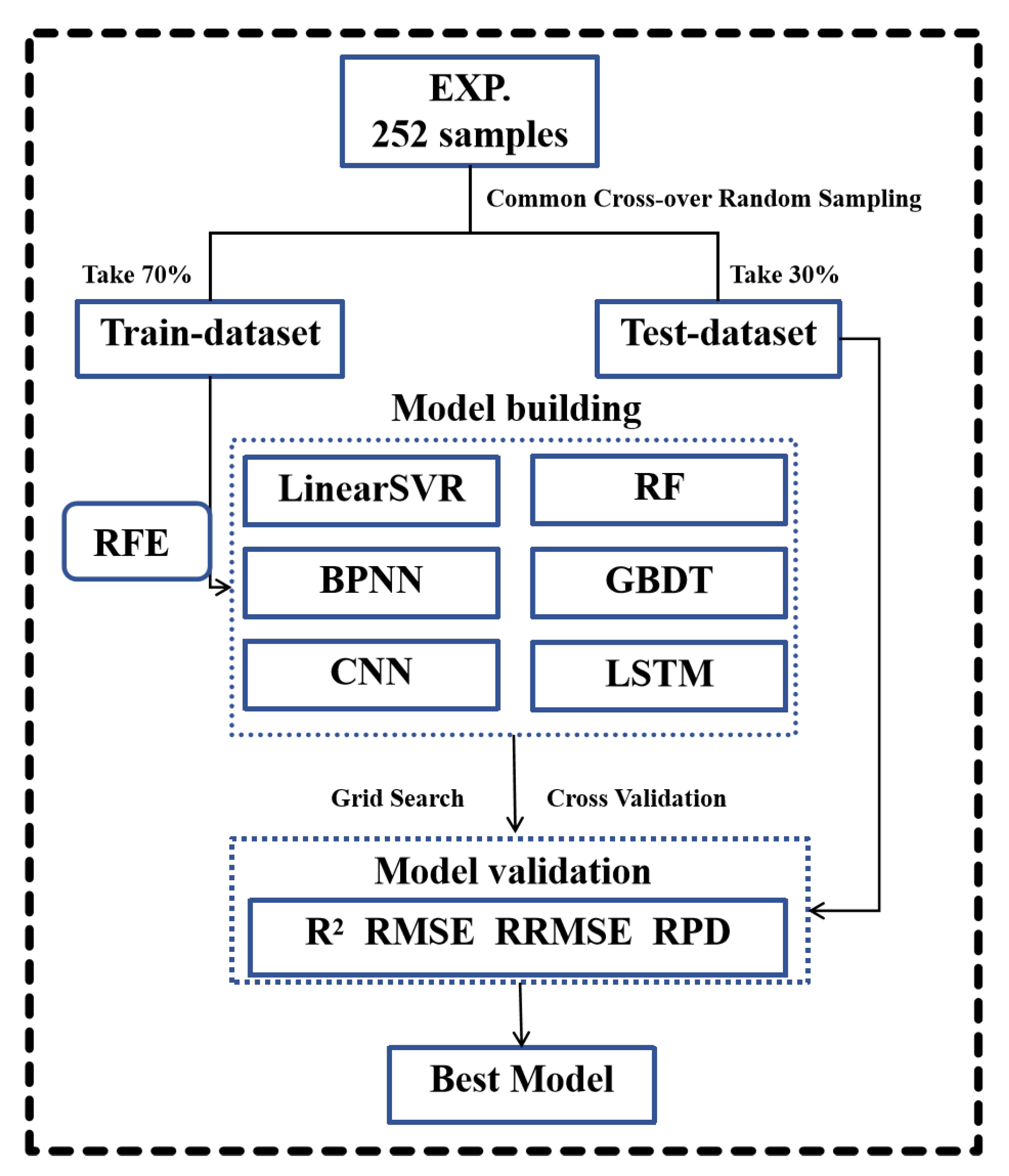
This study involves wheat nitrogen management experiments with four winter wheat varieties and four nitrogen application rates. Consequently, establishing the relationship between winter wheat canopy SPAD values and remote sensing variables became a complex task, posing substantial challenges in model development. The objective was to formulate a dynamic estimation model for winter wheat canopy SPAD values, customized for various cultivars and nitrogen application strategies. This model aimed to address challenges during vulnerable growth stages exposed to low-temperature stress, namely tillering, green-up, jointing, and booting. Leveraging UAV-based multispectral imagery, this research encompassed the extraction and construction of both VIs and TIs. Pearson correlation analysis was conducted between these variables and the measured SPAD values of winter wheat. Subsequently, Recursive Feature Elimination (RFE) was employed to select optimal subsets of VIs, TIs, and their fused combinations. These selected remote sensing variables were integrated into six machine learning algorithms, namely LinearSVR, RF, BPNN, GBDT, CNN, and LSTM. The goal was to establish winter wheat SPAD value estimation models. The models were then evaluated based on various performance metrics, culminating in identifying the optimal inversion model, which was further subjected to validation. The comprehensive methodology employed in this study addresses the complex and multifaceted nature of winter wheat SPAD value estimation. By integrating various approaches, from remote sensing to machine learning, the study demonstrates a systematic process for building reliable SPAD value estimation models capable of accommodating diverse cultivars and nitrogen application strategies. The findings provide valuable insights into optimizing agricultural management practices and enhancing winter wheat growth and yield outcomes.

4.1. Contribution of Different Remote Sensing Variables to Winter Wheat SPAD Value Prediction

4.1.1. Performance of Models Based on VIs

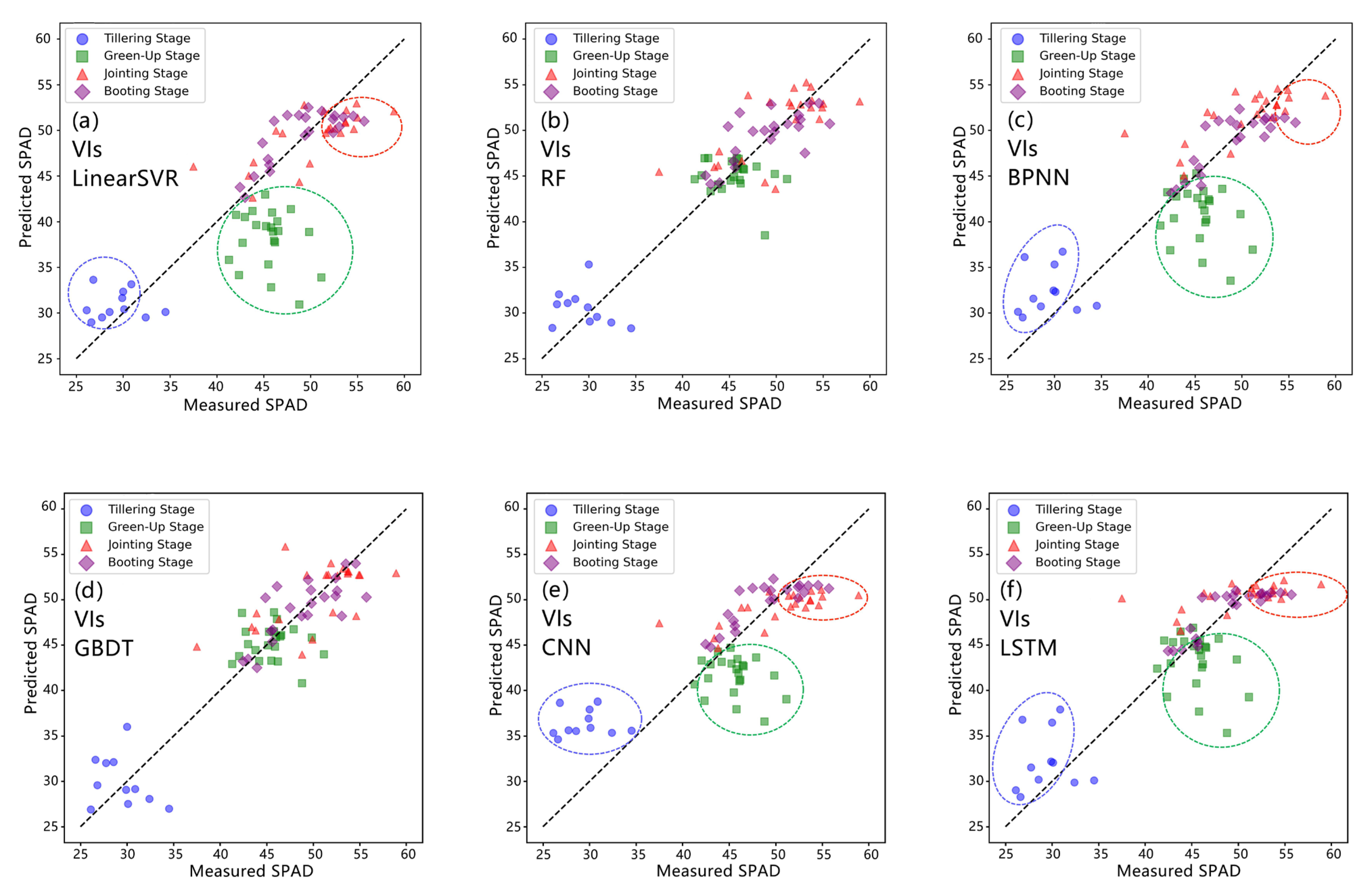
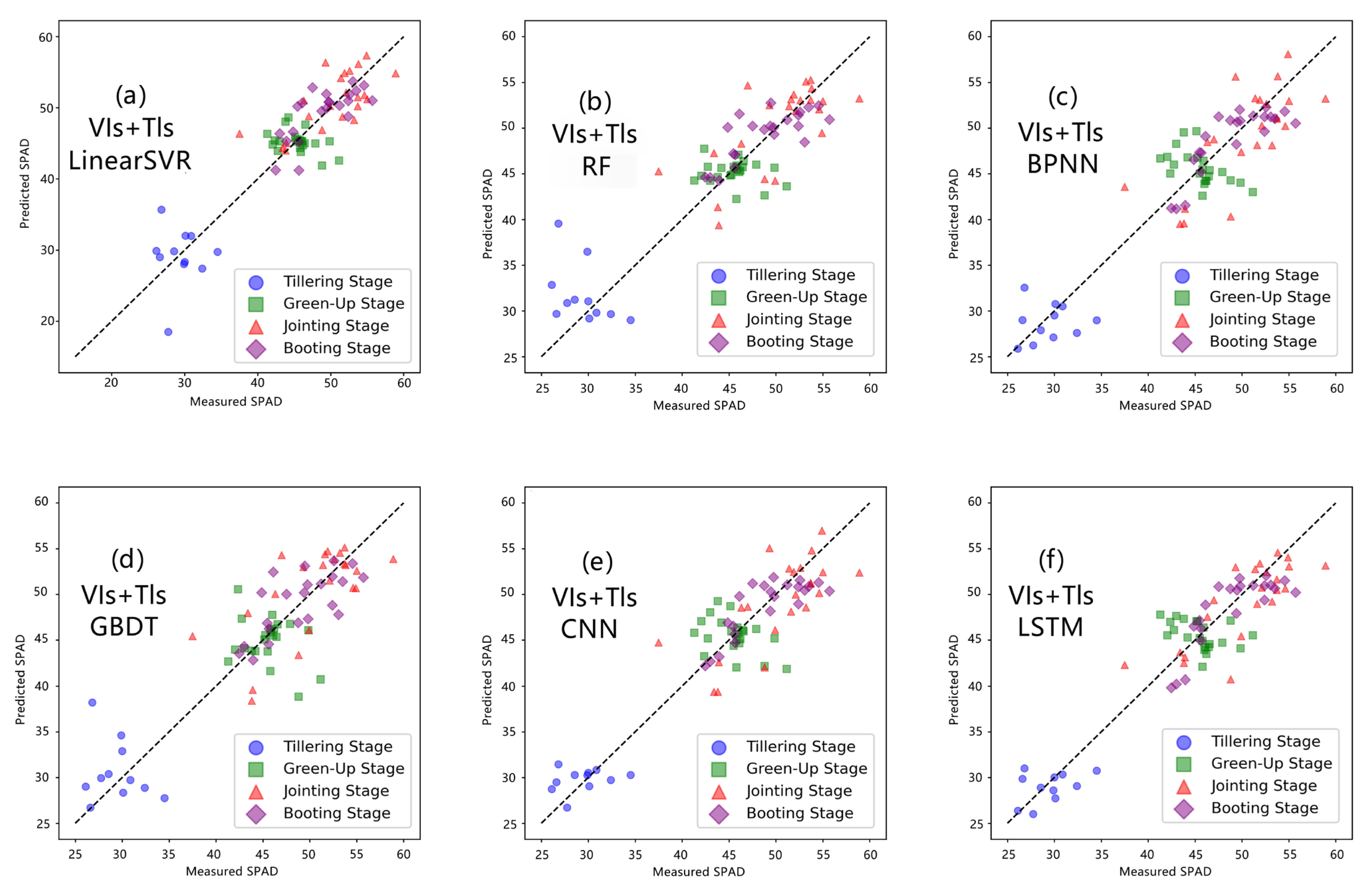
In the models established based on VIs, the performance of SPAD value estimation was assessed by comparing the estimated SPAD values obtained from each regression model with the corresponding measured values through scatter plots (Figure 9). As indicated by the data points covered by red circles, it is noteworthy that most regression methods underestimated the SPAD values during the jointing and booting stages of winter wheat. These underestimated data points often represent areas where winter wheat had higher density and canopy height. This phenomenon could be attributed to common saturation issues in optical remote sensing, particularly in moderate to high vegetation cover and yield [75,76,77].

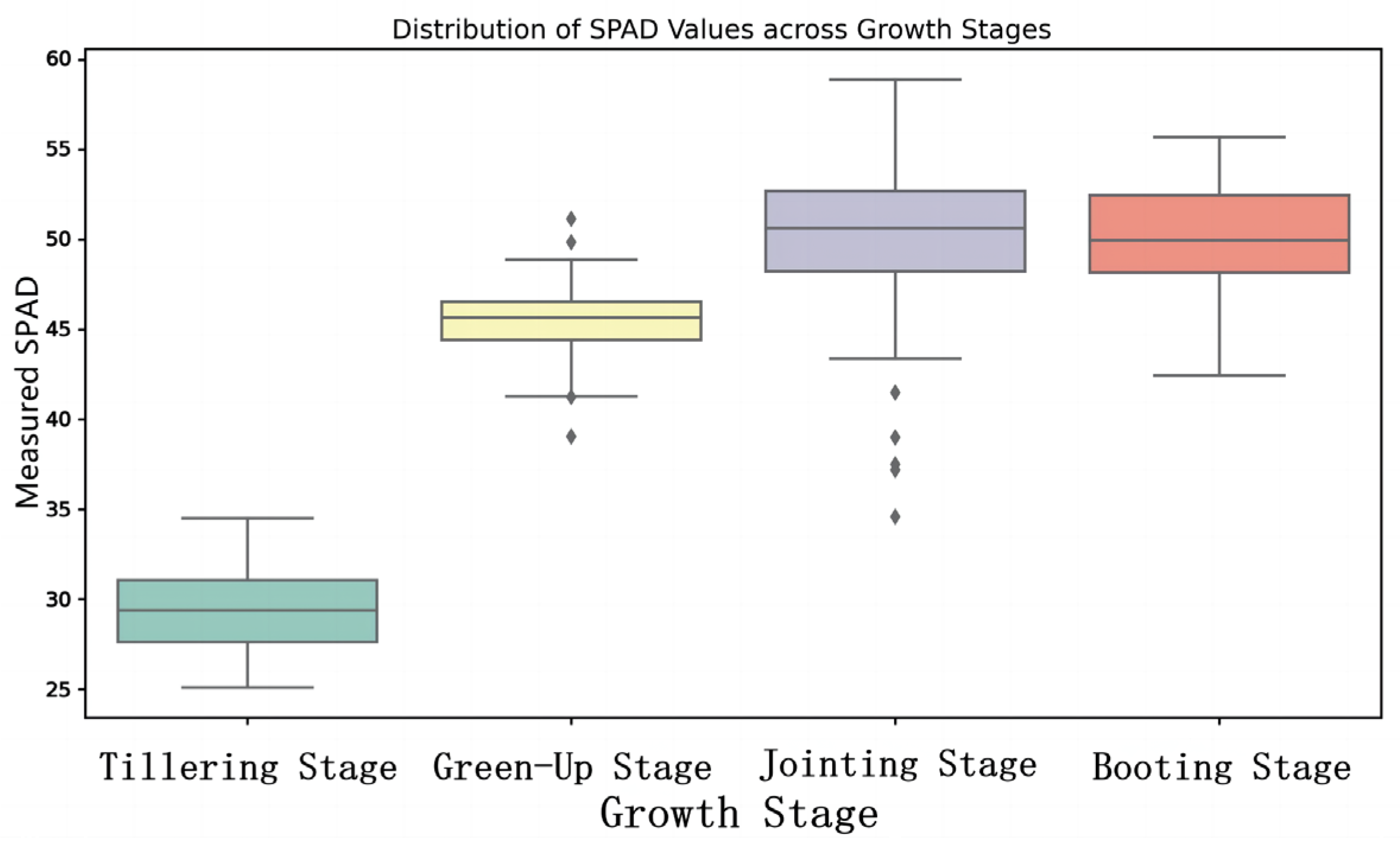
Furthermore, as evident from the data points covered by green circles, LinearSVR, BPNN, CNN, and LSTM underestimated the SPAD values during the green-up stage of winter wheat for most cases. This might be because the green-up stage marks the beginning of winter wheat growth in the subsequent year, following an extended dormancy period during the winter. The wheat plants deplete their nutrient reserves over this dormant period and require nutrient replenishment for subsequent growth and energy accumulation [75]. Consequently, there is significant variability in chlorophyll content across different varieties and nitrogen management strategies, rendering the relationship between winter wheat canopy SPAD values and VIs complex. Due to these intricate dynamics, machine learning models struggle to achieve perfect SPAD value estimation.

In the scatter plots, data points corresponding to the tillering stage of winter wheat, covered by blue circles, were often overestimated by most regression models. This could potentially be attributed to the fact that during the tillering stage, the vegetation cover of winter wheat is relatively low, with a significant amount of exposed soil, which can lead to an overestimation of SPAD values [78].

Compared to LinearSVR, CNN, and BPNN, the underestimation of SPAD values during the green-up stage is somewhat alleviated in LSTM and GBDT, and RF achieves the best estimation performance for this stage. Additionally, the underestimation of SPAD values during the jointing and booting stages, as well as the overestimation of SPAD values during the tillering stage, is also best captured by RF and GBDT. RF is relatively less influenced by light saturation compared to the other machine learning models. This observation somewhat implies its capability to manage peak information effectively [79]. Therefore, RF achieves the best winter wheat SPAD value estimation based on VIs, consistent with previous research findings [65,80].

4.1.2. Performance of Regression Models Based on TIs

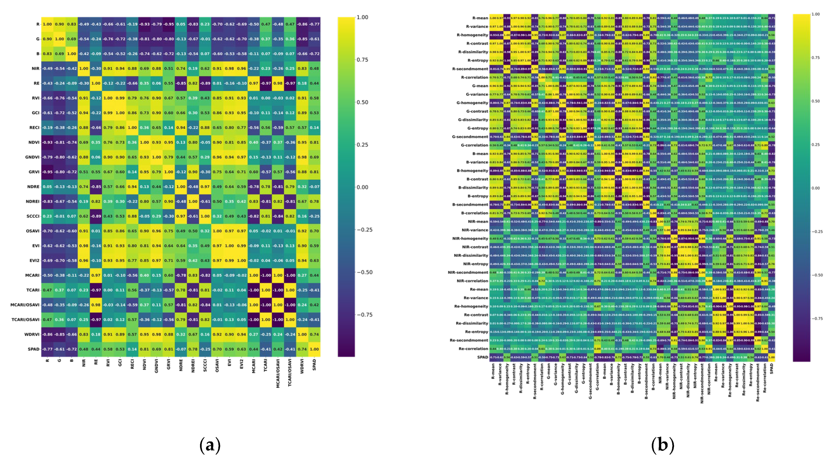
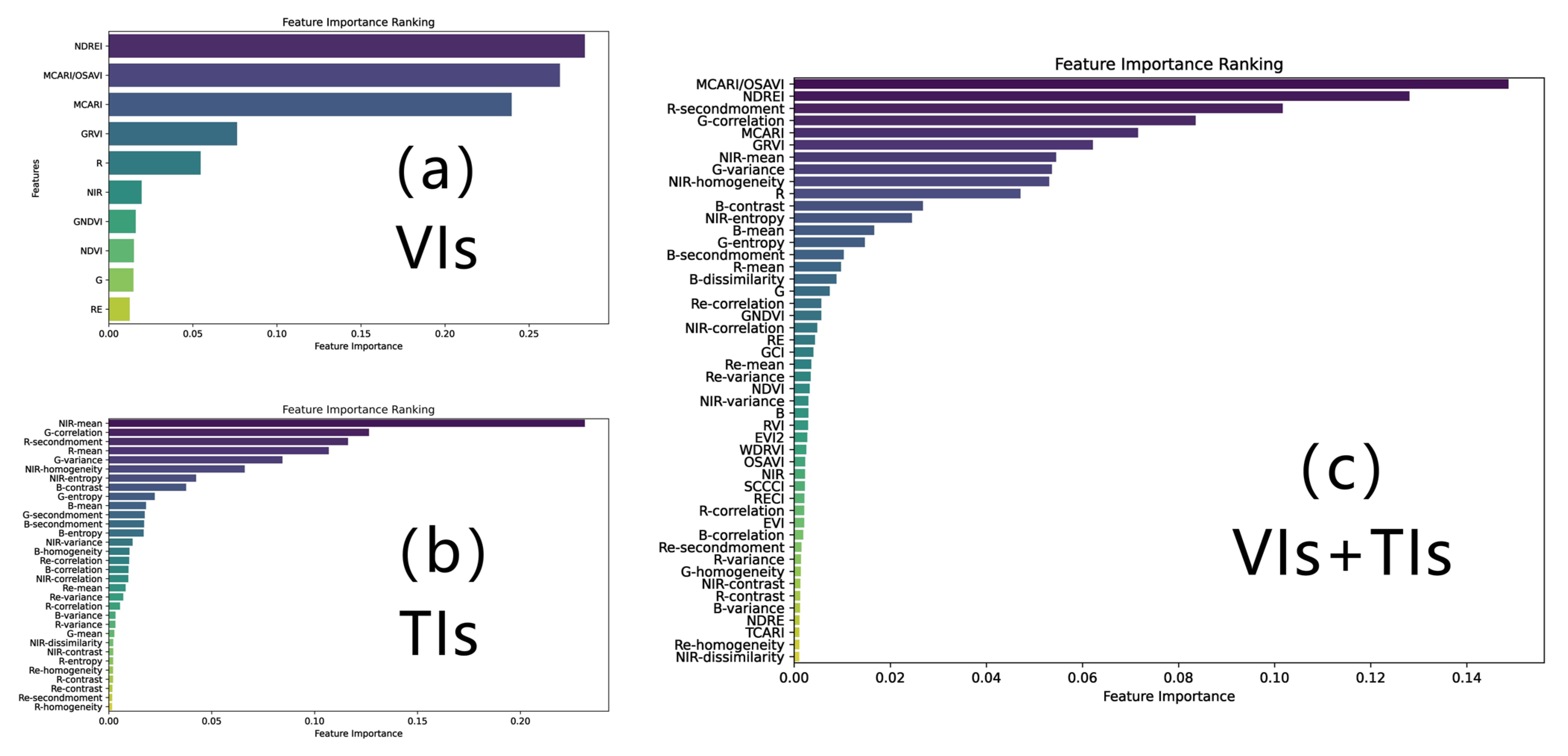
Through Pearson correlation analysis, we found that the texture index “Mean” extracted using GLCM exhibited good correlations with SPAD values across different bands. This aligns with the conclusions of Zheng et al. [81], who concluded that “mean” was the best TI for estimating rice biomass using various TIs. By integrating the “mean” texture index as an input, the accuracy and stability of the estimation model can be elevated, offering valuable insights for refining future methodologies and advancing wheat chlorophyll content estimation models.

In the construction of SPAD value estimation models, models based on TIs outperformed those based on VIs, indicating the substantial potential of TIs in predicting SPAD values. This finding aligns with Guo et al.’s research [44], which used multispectral images from UAVs to predict corn SPAD values by combining VIs and TIs. In comparison to VIs, TIs exhibited a stronger correlation with SPAD values.

However, in a study by Maitiniyazi et al. [77] involving the prediction of soybean yield through the fusion of multimodal data and deep learning from UAVs, it was shown that spectral information performed better in predicting soybean yield during the early growth stage of a single growth period, using images captured by UAVs. This study extracted various remote sensing variables, including TIs and Vis, for yield estimation. The results suggested that spectral information was superior to texture features in predicting soybean yield, indicating that texture features could be a potential alternative to VIs with reasonably good predictive accuracy. In contrast, texture information seemed to estimate physiological parameters during various growth stages of crops more effectively. This difference in findings could be attributed to several factors. On the one hand, there exists a strong correlation between chlorophyll content and plant photosynthesis. Plants with higher chlorophyll content exhibit elevated photosynthetic capacity and tend to accumulate a greater amount of photosynthetic products. Winter wheat with higher chlorophyll content often has larger leaves during the early growth stages [27]. As a result, remote sensing images display noticeable variations in texture among winter wheat samples with distinct SPAD values. Furthermore, our study involved different growth stages, various nitrogen management strategies, and four different winter wheat varieties, which contributed to more pronounced texture differences.

On the other hand, after RFE feature selection, all extracted TIs retained a significant number of features for subsequent modeling, whereas VIs retained only a small subset of features. This suggests that the unscreened VIs might have severe linear correlations and data redundancy between them [80]. The combination of these factors led to the better performance of models based on TIs in constructing SPAD value estimation models for winter wheat pre-heading stages.

4.1.3. Performance of Regression Models Based on Fusion of VIs and TIs

Consistent with our hypothesis, the overall trend of estimation accuracy among the six algorithms using different parameter combinations for modeling is as follows: fusion of VIs and TIs model > TIs model > VIs model. VIs provide the spectral information of winter wheat canopy, while TIs contribute spatial structural information. By fusing VIs and TIs, relevant information regarding winter wheat canopy SPAD values can be extracted from varying perspectives to enhance the accuracy of the model. This finding is congruent with the research by Zheng et al. [81], who improved the estimation of above-ground biomass in rice using a combination of UAV images, TIs, and VIs, as well as the results of Guo et al. [82], who integrated spectral and texture information for monitoring pear tree growth status using UAV remote sensing. Regardless of the modeling method used, multimodal data fusion consistently provides superior performance for the estimation model of winter wheat pre-heading stage SPAD values.

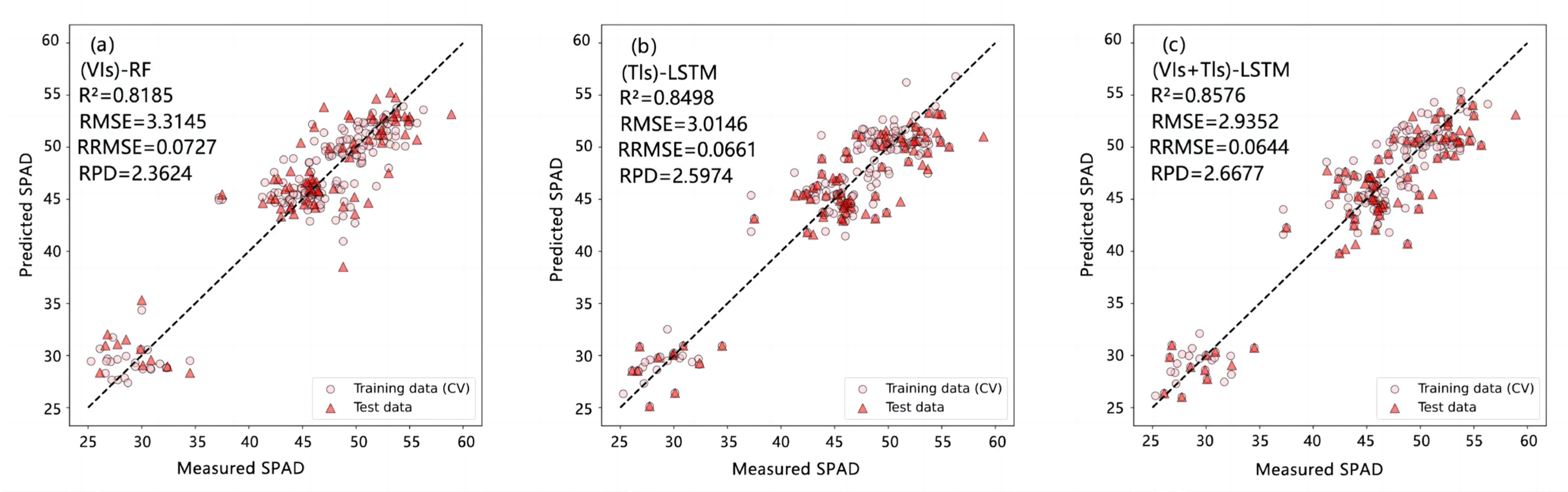
In establishing the SPAD value estimation model using the fusion of VIs and TIs, scatter plots were used to compare the estimated SPAD values obtained by each regression method with the corresponding measured values (Figure 10). It is worth noting that all regression methods considerably corrected the issues of underestimation and overestimation of winter wheat SPAD values observed in the model based solely on VIs. Fusing VIs and TIs could alleviate the saturation problem when using spectral information to estimate crop growth parameters. This can be attributed to the heterogeneity in VIs and TIs, which aligns with previous research findings [33,40].

Discrete data points during the tillering and green-up stages also showed significant improvement and the fitting effect between predicted and measured values was enhanced. By fusing multiple features, the model becomes adept at extracting pertinent information from diverse sources, which in turn diminishes the impact of noise and enhances the overall accuracy of chlorophyll content estimation [83].

4.2. Performance of the Optimal Estimation Model

The deep-learning-based estimation model LSTM fuses VIs and TIs and demonstrates remarkable performance in predicting winter wheat pre-heading stage SPAD values. According to Rossel et al. [74], LSTM achieved an RPD greater than 2.5 on the validation set in this study, indicating excellent estimation of winter wheat SPAD values. Furthermore, LSTM achieved the highest R² among all regression models and the lowest RMSE and RRMSE values. This implies that the model can effectively explain the variability of the target variable with minimal differences between predicted and actual winter wheat SPAD values. Hence, it stands as the optimal model for estimating SPAD values during the pre-heading stage of winter wheat. This observation aligns with the conclusions drawn by Liu et al. [78], who used UAV imagery and shallow and deep machine learning algorithms to estimate leaf area index. Their research indicated that deep machine learning models combined with multimodal data fusion could provide more accurate and reliable crop parameter estimation.

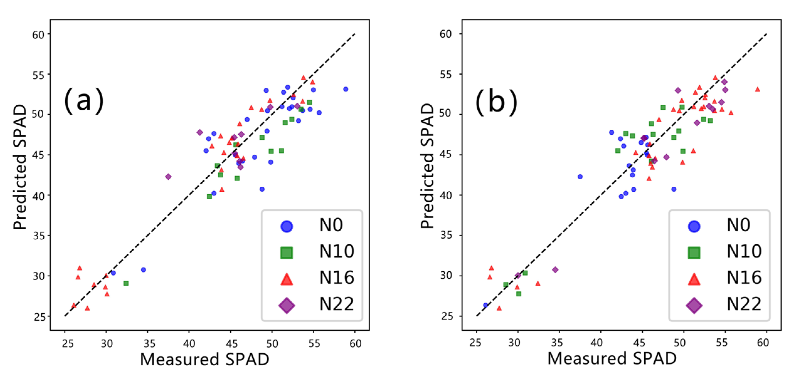
As shown in the inversion results (Figure 8), we tested the selected optimal model LSTM (fusing VIs and TIs) on the test dataset by different wheat varieties and nitrogen application levels. Among different wheat varieties (Table 6), NM 26 and YM 22 showed slightly poorer inversion results. Similarly, among different nitrogen levels (Table 7), N 0 exhibited slightly lower inversion results. However, most other varieties and nitrogen levels exhibited good inversion results. Both NM 26 and YM 22 are nitrogen-inefficient varieties. The considerable variation in chlorophyll content for these nitrogen-inefficient varieties, especially under lower nitrogen levels [84], presents a challenging task for the model due to the complexity of the relationship between canopy information and SPAD values.

In summary, as depicted in Figure 8 and Table 6 and Table 7, the newly constructed optimal regression model based on VIs and TIs, selected through RFE feature selection and established using LSTM, demonstrates good applicability and generalization across various winter wheat varieties and nitrogen management strategies. LSTM’s weight adjustments through backpropagation mitigate overfitting issues and enhance the model’s generalization ability [85]. This is particularly advantageous when dealing with datasets like winter wheat growth, where there may be noise or fluctuations in the data. The LSTM’s capacity to learn from errors and fine-tune its parameters ensures that it can effectively capture the underlying patterns without being overly influenced by noise. Additionally, LSTM excels in capturing long-term dependencies in the data, which is a critical factor in modeling winter wheat growth [86,87]. During the various growth stages of winter wheat, the condition of the crop may be influenced by multiple preceding periods. Furthermore, the complex nonlinear mapping relationships between the input features (such as VIs and TIs) and the target variable (SPAD values) are effectively handled by LSTM. This is essential because plant growth is a multifaceted process influenced by numerous interrelated variables.

The LSTM’s capacity to learn and model these intricate relationships aids in interpreting the nuanced and often nonlinear connections between the various factors and the growth of winter wheat. This makes it a powerful tool for accurately estimating SPAD values and, by extension, assessing the crop’s health and resilience during the pre-heading growth stage.

4.3. Limitations and Future Directions

While our research has achieved encouraging results in estimating winter wheat SPAD values, there are certain limitations that need to be addressed. Our models primarily focus on the pre-heading stages of winter wheat growth, leaving gaps in modeling the entire growth cycle, including the heading stage. This could impact the accuracy of our models when predicting crop parameters throughout the complete growth period.

To overcome these limitations and achieve greater advancements, our future efforts will be directed toward establishing models applicable to the entire growth cycle of winter wheat, encompassing not only the pre-heading but also the post-heading stages. This endeavor would necessitate considering the influence of different growth phases on SPAD values. It may require incorporating additional features and data sources, such as ground-level observations and meteorological data. Such enhancements would contribute to the overall comprehensiveness and precision of the models, providing a more holistic understanding of winter wheat growth dynamics and enabling more accurate parameter estimation throughout the entire growth cycle.

5. Conclusions

The findings of this study demonstrate that integrating VIs and TIs from UAV-based multispectral imagery allows for more accurate monitoring of winter wheat SPAD values in the middle and lower reaches of the Yangtze River region. This approach enables the construction of SPAD value estimation models that apply to various crucial growth stages before heading (tillering, green-up, jointing, and booting), multiple cultivars, and different nitrogen management strategies. Overall, the estimation accuracy follows the order of the fused VIs and TIs model, TIs model, and VIs model.

The model established based on VIs for predicting winter wheat pre-heading canopy SPAD values exhibits both overestimation and underestimation issues. Underestimation occurs under high vegetation cover conditions due to spectral saturation, while periods with more exposed soil tend to overestimate SPAD values. Additionally, accurate SPAD value estimation during the regrowth phase of the second-year winter wheat, known as the “green-up” stage, proves challenging.

Models based on TIs outperform those based on VIs, showcasing substantial potential in SPAD value prediction. The texture index “Mean”, extracted using the GLCM method, exhibits a good correlation with SPAD values across various wavelength bands. Compared to VIs, TIs exhibit a closer association with SPAD values, offering a potential alternative to spectral variables with considerable predictive accuracy.

The newly constructed optimal regression model integrates fused spectral and TIs through RFE feature selection and utilizes LSTM, demonstrating good applicability and generalization across different winter wheat cultivars and nitrogen management strategies. This model accurately estimates pre-heading canopy SPAD values. Feature fusion leads to the model’s capability to extract pertinent information from diverse sources, effectively mitigating the influence of noise and thereby augmenting the overall accuracy of chlorophyll content estimation. Moreover, it significantly corrects the issues of underestimation and overestimation seen in models based solely on VIs.

This research provides valuable insights for farmers to adjust agricultural management practices promptly, thereby mitigating the hazards posed by pre-heading cold damage and improving the growth and yield of winter wheat. Future endeavors will focus on optimizing and enhancing the multi-feature fusion model, introducing the post-heading growth stages of winter wheat, and incorporating additional features to improve further the accuracy and applicability of the SPAD value estimation model. This will facilitate more comprehensive and precise monitoring and assessment of winter wheat growth status.

References

1. Jones, R.A.; Qualset, C.O. Breeding crops for environmental stress tolerance. Appl. Genet. Eng. Crop Improv. 1984, 10, 305–340. [Google Scholar]
2. Li, C.Y.; Yang, J.; Zhang, Y.X.; Yao, M.H.; Zhu, X.K.; Guo, W.S. Retrieval effects of remedial fertilizer after freeze injury on wheat yield and its mechanism at the tillering stage. Sci. Agric. Sin. 2017, 50, 1781–1791, (In Chinese with English Abstract). [Google Scholar]
3. Shi, Z.L.; Guo, J.K. Effects of cold damage on wheat growth and development and yield. J. Hebei Agric. Sci. 1997, 1, 1–4, (In Chinese with English Abstract). [Google Scholar]
4. Liu, C.; Wang, W.L.; Zhao, C.; Li, G.H.; Xu, K.; Huo, Z.Y. Current status and prospects of research on late spring frost in wheat. Jiangsu J. Agric. Sci. 2022, 38, 1115–1122, (In Chinese with English Abstract). [Google Scholar]
5. Zhao, G.; Shen, S.H.; Chu, R.H. Assessment of the degree of late spring frost occurrence in Jiangsu Province. Jiangsu Agric. Sci. 2018, 46, 243–247, (In Chinese with English Abstract). [Google Scholar]
6. Yang, W.G.; Huang, Y.X.; Liu, K.Q.; Fan, J.J.; Meng, C.L. Study on meteorological indicators and classification of late spring frost. Hubei Agric. Sci. 2018, 612, 51–55, (In Chinese with English Abstract). [Google Scholar]
7. Liu, F.F.; Wan, Y.X.; Cao, W.X.; Zhang, Q.Q.; Li, Y.; Li, Y.; Zhang, P.Z. Research progress on identification of late spring frost resistance in wheat. J. Plant Genet. Resour. 2021, 22, 1193–1199, (In Chinese with English Abstract). [Google Scholar]
8. Gao, Y.; Zhang, Y.X.; Ma, Q.; Su, S.N.; Li, C.Y.; Din, J.F.; Zhu, M.; Zhu, X.K.; Guo, W.S. Effects of spring low temperature on wheat pollen fertility and grain number formation. Acta Agron. Sin. 2021, 47, 104–115, (In Chinese with English Abstract). [Google Scholar] [CrossRef]
9. Ren, D.C.; Hu, X.; Huang, S.H.; Ge, J.; Zhao, J.L.; Zhu, P.P.; Zhang, F.J. Effects of late spring frost on yield traits of different types of wheat. Henan Agric. Sci. 2011, 40, 57, (In Chinese with English Abstract). [Google Scholar]
10. Wang, C.Y.; Li, M.S.; Hu, X.; Wang, D.L.; Ji, T.J. Resistance of winter wheat to late spring frost in the Huang-Huai area. J. Nat. Disasters. 2006, 15, 211–215, (In Chinese with English Abstract). [Google Scholar]
11. Wu, Y.F.; Zhong, X.L.; Hu, X.; Ren, D.; Lv, G.; Wei, C.; Song, J. Frost affects grain yield components in winter wheat. N. Z. J. Crop Hort. Sci. 2014, 42, 194–204. [Google Scholar] [CrossRef]
12. Si, T.; Wang, X.; Wu, L.; Zhao, C.; Zhang, L.; Mei, H.; Cai, J.; Zhou, Q.; Dai, T.; Zhu, J.; et al. Nitric oxide and hydrogen peroxide mediate wounding-induced freezing tolerance through modifications in photosystem and antioxidant system in wheat. Front. Plant Sci. 2017, 8, 1284. [Google Scholar] [CrossRef] [PubMed]
13. Li, K.N.; Yang, X.G.; Mu, C.Y.; Xu, H.J.; Chen, F. Potential impacts of global climate warming on China’s planting system VIII: Effects of climate change on the planting boundary of winter-spring varieties of Chinese winter wheat. Chin. Agric. Sci. 2013, 46, 1583–1594, (In Chinese with English Abstract). [Google Scholar]
14. Poorter, H.; Niklas, K.J.; Reich, P.B.; Oleksyn, J.; Poot, P.; Mommer, L. Biomass allocation to leaves, stems and roots: Meta-analyses of interspecific variation and environmental control. New Phytol. 2012, 193, 30–50. [Google Scholar] [CrossRef]
15. Gitelson, A.A.; Merzlyak, M.N. Remote sensing of chlorophyll concentration in higher plant leaves. Adv. Space Res. 1998, 22, 689–692. [Google Scholar] [CrossRef]
16. Bojović, B.; Marković, A. Correlation between nitrogen and chlorophyll content in wheat (Triticum aestivum L.). Kragujev. J. Sci. 2009, 31, 69–74. [Google Scholar]
17. Singh, B.; Singh, Y.; Ladha, J.K.; Bronson, K.F. Chlorophyll meter- and leaf color chart-based nitrogen management for rice and wheat in Northwestern India. Agron. J. 2002, 94, 821–829. [Google Scholar] [CrossRef]
18. Hoel, B.O.; Solhaug, K.A. Effect of irradiance on chlorophyll estimation with the Minolta SPAD-502 leaf chlorophyll meter. Ann. Bot. 1998, 82, 389–392. [Google Scholar] [CrossRef]
19. Wood, C.W.; Reeves, D.W.; Himelrick, D.G. Relationships between chlorophyll meter readings and leaf chlorophyll concentration, N status, and crop yield: A review. Proc. Agron. Soc. N. Z. 1993, 23, 1–9. [Google Scholar]
20. Debaeke, P.; Rouet, P.; Justes, E. Relationship between the normalized SPAD index and the nitrogen nutrition index: Application to durum wheat. J. Plant Nutr. 2006, 29, 75–92. [Google Scholar] [CrossRef]
21. Reeves, D.W.; Mask, P.L.; Wood, C.W.; Delaney, D.P. Determination of wheat nitrogen status with hand-held chlorophyll meter: Influence of management practices. J. Plant Nutr. 1993, 16, 781–796. [Google Scholar] [CrossRef]
22. Zhao, C.; Jiang, A.; Huang, W.; Liu, K.; Liu, L.; Wang, J. Evaluation of variable-rate nitrogen recommendation of winter wheat based on SPAD chlorophyll meter measurement. N. Z. J. Agric. Res. 2007, 50, 735–741. [Google Scholar]
23. Ghosh, M.; Swain, D.K.; Jha, M.K.; Tewari, V.K.; Bohra, A. Optimizing chlorophyll meter (SPAD) reading to allow efficient nitrogen use in rice and wheat under rice-wheat cropping system in eastern India. Plant Prod. Sci. 2020, 23, 270–285. [Google Scholar] [CrossRef]
24. Zhang, K.; Yuan, Z.; Yang, T.; Lu, Z.; Cao, Q.; Tian, Y.; Zhu, Y.; Cao, W.; Liu, X. Chlorophyll meter-based nitrogen fertilizer optimization algorithm and nitrogen nutrition index for in-season fertilization of paddy rice. Agron. J. 2020, 112, 288–300. [Google Scholar] [CrossRef]
25. Fox, R.H.; Piekielek, W.P.; Macneal, K.M. Using a chlorophyll meter to predict nitrogen fertilizer needs of winter wheat. Commun. Soil Sci. Plant Anal. 1994, 25, 171–181. [Google Scholar] [CrossRef]
26. Wu, Q.; Zhang, Y.; Zhao, Z.; Xie, M.; Hou, D. Estimation of Relative Chlorophyll Content in Spring Wheat Based on Multi-Temporal UAV Remote Sensing. Agronomy 2023, 13, 211. [Google Scholar] [CrossRef]
27. Wang, Y.; Tan, S.; Jia, X.; Qi, L.; Liu, S.; Lu, H.; Wang, C.; Liu, W.; Zhao, X.; He, L.; et al. Estimating Relative Chlorophyll Content in Rice Leaves Using Unmanned Aerial Vehicle Multi-Spectral Images and Spectral–Textural Analysis. Agronomy 2023, 13, 1541. [Google Scholar] [CrossRef]
28. Wang, P.; Wang, L.; Leung, H.; Zhang, G. Super-resolution mapping based on spatial–spectral correlation for spectral imagery. IEEE Trans. Geosci. Remote Sens. 2020, 59, 2256–2268. [Google Scholar] [CrossRef]
29. Shang, X.; Song, M.; Wang, Y.; Yu, C.; Yu, H.; Li, F.; Chang, C.I. Target-constrained interference-minimized band selection for hyperspectral target detection. IEEE Trans. Geosci. Remote Sens. 2020, 59, 6044–6064. [Google Scholar] [CrossRef]
30. Shen, L.; Gao, M.; Yan, J.; Wang, Q.; Shen, H. Winter Wheat SPAD Value Inversion Based on Multiple Pretreatment Methods. Remote Sens. 2022, 14, 4660. [Google Scholar] [CrossRef]
31. Fu, Y.; Yang, G.; Wang, J.; Song, X.; Feng, H. Winter wheat biomass estimation based on spectral indices, band depth analysis and partial least squares regression using hyperspectral measurements. Comput. Electron. Agric. 2014, 100, 51–59. [Google Scholar] [CrossRef]
32. Nguy-Robertson, A.; Gitelson, A.; Peng, Y.; Viña, A.; Arkebauer, T.; Rundquist, D. Green leaf area index estimation in maize and soybean: Combining vegetation indices to achieve maximal sensitivity. Agron. J. 2012, 104, 1336–1347. [Google Scholar] [CrossRef]
33. Sibanda, M.; Mutanga, O.; Rouget, M.; Kumar, L. Estimating biomass of native grass grown under complex management treatments using worldview-3 spectral derivatives. Remote Sens. 2017, 9, 55. [Google Scholar] [CrossRef]
34. Sun, H.; Li, M.; Zhao, Y.; Wang, X.; Li, X. The spectral characteristics and chlorophyll content at winter wheat growth stages. Spectrosc. Spectr. Anal. 2010, 30, 192–196. [Google Scholar]
35. Zhu, Y.; Liu, J.; Tao, X.; Su, X.; Li, W.; Zha, H.; Wu, W.; Li, X. A Three-Dimensional Conceptual Model for Estimating the Above-Ground Biomass of Winter Wheat Using Digital and Multispectral Unmanned Aerial Vehicle Images at Various Growth Stages. Remote Sens. 2023, 15, 3332. [Google Scholar] [CrossRef]
36. Liu, X.; Wu, X.; Peng, Y.; Mo, J.; Fang, S.; Gong, Y.; Zhu, R.; Wang, J.; Zhang, C. Application of UAV-retrieved canopy spectra for remote evaluation of rice full heading date. Sci. Remote Sens. 2023, 7, 100090. [Google Scholar] [CrossRef]
37. Wang, J.; Zhou, Q.; Shang, J.; Liu, C.; Zhuang, T.; Ding, J.; Xian, Y.; Zhao, L.; Wang, W.; Zhou, G.; et al. UAV-and machine learning-based retrieval of wheat SPAD values at the overwintering stage for variety screening. Remote Sens. 2021, 13, 5166. [Google Scholar] [CrossRef]
38. Haboudane, D.; Miller, J.R.; Tremblay, N.; Zarco-Tejada, P.J.; Dextraze, L. Integrated narrow-band vegetation indices for prediction of crop chlorophyll content for application to precision agriculture. Remote Sens. Environ. 2002, 81, 416–426. [Google Scholar] [CrossRef]
39. De Grandi, G.D.; Lucas, R.M.; Kropacek, J. Analysis by wavelet frames of spatial statistics in SAR data for characterizing structural properties of forests. IEEE Trans. Geosci. Remote Sens. 2008, 47, 494–507. [Google Scholar] [CrossRef]
40. Mutanga, O.; Skidmore, A.K. Narrow band vegetation indices overcome the saturation problem in biomass estimation. Int. J. Remote Sens. 2004, 25, 3999–4014. [Google Scholar] [CrossRef]
41. Mishra, P.; Cordella, C.B.Y.; Rutledge, D.N.; Barreiro, P.; Roger, J.M.; Diezma, B. Application of independent components analysis with the JADE algorithm and NIR hyperspectral imaging for revealing food adulteration. J. Food Eng. 2016, 168, 7–15. [Google Scholar] [CrossRef]
42. Cheng, W.W.; Sun, D.W.; Pu, H.B.; Liu, Y. Integration of spectral and textural data for enhancing hyperspectral prediction of K value in pork meat. LWT-Food Sci. Technol. 2016, 72, 322–329. [Google Scholar] [CrossRef]
43. Zhang, C.; Guo, C.T.; Liu, F.; Kong, W.; He, Y.; Lou, B.G. Hyperspectral imaging analysis for ripeness evaluation of strawberry with support vector machine. J. Food Eng. 2016, 179, 11–18. [Google Scholar] [CrossRef]
44. Guo, Y.; Chen, S.; Li, X.; Cunha, M.; Jayavelu, S.; Cammarano, D.; Fu, Y. Machine learning-based approaches for predicting SPAD values of maize using multi-spectral images. Remote Sens. 2022, 14, 1337. [Google Scholar] [CrossRef]
45. Yang, K.; Gong, Y.; Fang, S.; Duan, B.; Yuan, N.; Peng, Y.; Wu, X.; Zhu, R. Combining spectral and texture features of UAV images for the remote estimation of rice LAI throughout the entire growing season. Remote Sens. 2021, 13, 3001. [Google Scholar] [CrossRef]
46. Li, H.; Liu, L.; Wang, Z.; Yang, J.; Zhang, J. Agronomic and physiological performance of high-yielding wheat and rice in the lower reaches of the Yangtze River of China. Field Crops Res. 2012, 133, 119–129. [Google Scholar] [CrossRef]
47. Large, E.C. Growth stages in cereals. Illustration of the Feekes scale. Plant Pathol. 1954, 3, 128–129. [Google Scholar] [CrossRef]
48. Jay, S.; Gorretta, N.; Morel, J.; Maupas, F.; Bendoula, R.; Rabatel, G.; Dutartre, D.; Comar, A.; Baret, F. Estimating leaf chlorophyll content in sugar beet canopies using millimeter-to centimeter-scale reflectance imagery. Remote Sens. Environ. 2017, 198, 173–186. [Google Scholar] [CrossRef]
49. Haralick, R.M.; Shanmugam, K.; Dinstein, I.H. Textural features for image classification. IEEE Trans. Syst. Man Cybern. 1973, 6, 610–621. [Google Scholar] [CrossRef]
50. Hall-Beyer, M. Practical guidelines for choosing GLCM textures to use in landscape classification tasks over a range of moderate spatial scales. Int. J. Remote Sens. 2017, 38, 1312–1338. [Google Scholar] [CrossRef]
51. Tucker, C.J. Red and photographic infrared linear combinations for monitoring vegetation. Remote Sens. Environ. 1979, 8, 127–150. [Google Scholar] [CrossRef]
52. Gitelson, A.A.; Viña, A.; Ciganda, V.; Ciganda, V.S.; Rundquist, D.C.; Arkebauer, T.J. Remote estimation of canopy chlorophyll content in crops. Geophys. Res. Lett. 2005, 32, L08403. [Google Scholar] [CrossRef]
53. Rouse, J.W.; Haas, R.H.; Schell, J.A.; Deering, D.W. Monitoring vegetation systems in the Great Plains with ERTS. NASA Spec. Publ. 1974, 351, 309. [Google Scholar]
54. Gitelson, A.A.; Gritz, Y.; Merzlyak, M.N. Relationships between leaf chlorophyll content and spectral reflectance and algorithms for non-destructive chlorophyll assessment in higher plant leaves. J. Plant Physiol. 2003, 160, 271–282. [Google Scholar] [CrossRef] [PubMed]
55. Gitelson, A.A.; Merzlyak, M.N. Remote estimation of chlorophyll content in higher plant leaves. Int. J. Remote Sens. 1997, 18, 2691–2697. [Google Scholar] [CrossRef]
56. Hassan, M.A.; Yang, M.; Rasheed, A.; Jin, X.; Xiao, Y.; He, Z. Time-series multispectral indices from unmanned aerial vehicle imagery reveal senescence rate in bread wheat. Remote Sens. 2018, 10, 809. [Google Scholar] [CrossRef]
57. Raper, T.B.; Varco, J.J. Canopy-scale wavelength and vegetative index sensitivities to cotton growth parameters and nitrogen status. Precis. Agric. 2015, 16, 62–76. [Google Scholar] [CrossRef]
58. Huete, A.; Didan, K.; Miura, T.; Rodrigurz, E.P.; Gao, X.; Ferreira, L.G. Overview of the radiometric and biophysical performance of the MODIS vegetation indices. Remote Sens. Environ. 2002, 83, 195–213. [Google Scholar] [CrossRef]
59. Jiang, Z.; Huete, A.R.; Didan, K.; Miura, T. Development of a two-band enhanced vegetation index without a blue band. Remote Sens. Environ. 2008, 112, 3833–3845. [Google Scholar] [CrossRef]
60. Rondeaux, G.; Steven, M.; Baret, F. Optimization of soil-adjusted vegetation indices. Remote Sens. Environ. 1996, 55, 95–107. [Google Scholar] [CrossRef]
61. Daughtry, C.S.T.; Walthall, C.L.; Kim, M.S.; Colstoun, E.B.; McMurtrey, J.E. Estimating corn leaf chlorophyll concentration from leaf and canopy reflectance. Remote Sens. Environ. 2000, 74, 229–239. [Google Scholar] [CrossRef]
62. Gitelson, A.A. Wide dynamic range vegetation index for remote quantification of biophysical characteristics of vegetation. J. Plant Physiol. 2004, 161, 165–173. [Google Scholar] [CrossRef]
63. Chen, L.; Xing, M.; He, B.; Wang, J.; Shang, J.; Huang, X.; Xu, M. Estimating soil moisture over winter wheat fields during the growing season using machine-learning methods. IEEE J. Sel. Top. Appl. Earth Obs. Remote Sens. 2021, 14, 3706–3718. [Google Scholar] [CrossRef]
64. Denil, M.; Shakibi, B.; Dinh, L.; Ranzato, M.; Freitas, N. Predicting parameters in deep learning. Adv. Neural Inf. Process. Syst. 2013, 26. [Google Scholar]
65. Yin, Q.; Zhang, Y.; Li, W.; Wang, J.; Wang, W.; Ahmad, I.; Zhou, G.; Huo, Z. Estimation of Winter Wheat SPAD Values Based on UAV Multispectral Remote Sensing. Remote Sens. 2023, 15, 3595. [Google Scholar] [CrossRef]
66. Ho, C.H.; Lin, C.J. Large-scale linear support vector regression. J. Mach. Learn. Res. 2012, 13, 3323–3348. [Google Scholar]
67. Belgiu, M.; Drăguţ, L. Random forest in remote sensing: A review of applications and future directions. ISPRS J. Photogramm. Remote Sens. 2016, 114, 24–31. [Google Scholar] [CrossRef]
68. Heermann, P.D.; Khazenie, N. Classification of multispectral remote sensing data using a back-propagation neural network. IEEE Trans. Geosci. Remote Sens. 1992, 30, 81–88. [Google Scholar] [CrossRef]
69. Mansaray, L.R.; Zhang, K.; Kanu, A.S. Dry biomass estimation of paddy rice with Sentinel-1A satellite data using machine learning regression algorithms. Comput. Electron. Agric. 2020, 176, 105674. [Google Scholar] [CrossRef]
70. Tanabe, R.; Matsui, T.; Tanaka, T.S.T. Winter wheat yield prediction using convolutional neural networks and UAV-based multispectral imagery. Field Crops Res. 2023, 291, 108786. [Google Scholar] [CrossRef]
71. Sherstinsky, A. Fundamentals of recurrent neural network (RNN) and long short-term memory (LSTM) network. Physica D Nonlinear Phenom. 2020, 404, 132306. [Google Scholar] [CrossRef]
72. Zha, H.; Miao, Y.; Wang, T.; Li, Y.; Zhang, J.; Sun, W.; Feng, Z.; Kusnierek, K. Improving unmanned aerial vehicle remote sensing-based rice nitrogen nutrition index prediction with machine learning. Remote Sens. 2020, 12, 215. [Google Scholar] [CrossRef]
73. Williams, P.C. Variables affecting near-infrared reflectance spectroscopic analysis. In Near-Infrared Technology in the Agricultural and Food Industries; Williams, P.C., Norris, K., Eds.; American Association of Cereal Chemists, Inc.: St. Paul, MN, USA, 1987; pp. 143–167. [Google Scholar]
74. Viscarra Rossel, R.; Taylor, H.J.; Mcbratney, A.B. Multivariate calibration of hyperspectral γ-ray energy spectra for proximal soil sensing. Eur. J. Soil Sci. 2007, 58, 343–353. [Google Scholar] [CrossRef]
75. Becker-Reshef, I.; Vermote, E.; Lindeman, M.; Justice, C. A generalized regression-based model for forecasting winter wheat yields in Kansas and Ukraine using MODIS data. Remote Sens. Environ. 2010, 114, 1312–1323. [Google Scholar] [CrossRef]
76. Vergara-Díaz, O.; Zaman-Allah, M.A.; Masuka, B.; Hornero, A.; Zarco-Tejada, P.J.; Prasanna, B.M.; Cairns, J.E.; Araus, J.L. A novel remote sensing approach for prediction of maize yield under different conditions of nitrogen fertilization. Front. Plant Sci. 2016, 7, 666. [Google Scholar] [CrossRef]
77. Maimaitijiang, M.; Sagan, V.; Sidike, P.; Hartling, S.; Esposito, F.; Fritschi, F.B. Soybean yield prediction from UAV using multimodal data fusion and deep learning. Remote Sens. Environ. 2020, 237, 111599. [Google Scholar] [CrossRef]
78. Liu, S.; Jin, X.; Nie, C.; Wang, S.; Yu, X.; Cheng, M.; Shao, M.; Wang, Z.; Tuohuti, N.; Bai, Y.; et al. Estimating leaf area index using unmanned aerial vehicle data: Shallow vs. deep machine learning algorithms. Plant Physiol. 2021, 187, 1551–1576. [Google Scholar] [CrossRef]
79. Ding, F.; Li, C.; Zhai, W.; Fei, S.; Cheng, Q.; Chen, Z. Estimation of nitrogen content in winter wheat based on multi-source data fusion and machine learning. Agriculture 2022, 12, 1752. [Google Scholar] [CrossRef]
80. Zhai, W.; Li, C.; Cheng, Q.; Ding, F.; Chen, Z. Exploring Multisource Feature Fusion and Stacking Ensemble Learning for Accurate Estimation of Maize Chlorophyll Content Using Unmanned Aerial Vehicle Remote Sensing. Remote Sens. 2023, 15, 3454. [Google Scholar] [CrossRef]
81. Zheng, H.; Cheng, T.; Zhou, M.; Li, D.; Yao, X.; Tian, Y.; Cao, W.; Zhu, Y. Improved estimation of rice aboveground biomass combining textural and spectral analysis of UAV imagery. Precis. Agric. 2019, 20, 611–629. [Google Scholar] [CrossRef]
82. Guo, Y.; Chen, S.; Wu, Z.; Wang, S.; Bryant, C.; Senthilnath, J.; Cunha, M.; Fu, Y.H. Integrating spectral and textural information for monitoring the growth of pear trees using optical images from the UAV platform. Remote Sens. 2021, 13, 1795. [Google Scholar] [CrossRef]
83. Cheng, M.; Jiao, X.; Liu, Y.; Shao, M.; Yu, X.; Bai, Y.; Wang, Z.; Wang, S.; Tuohuti, N.; Liu, S.; et al. Estimation of soil moisture content under high maize canopy coverage from UAV multimodal data and machine learning. Agric. Water Manag. 2022, 264, 107530. [Google Scholar] [CrossRef]
84. Zhang, H.; Chen, Y.Q.; Ren, J.Y.; Yang, H.K.; Fan, G.Q. Selection of Nitrogen-Efficient Wheat Varieties and Construction of Index System in Southwest Wheat Area at Seedling Stage. J. Sichuan Agric. Univ. 2022, 40, 10–18+27, (In Chinese with English Abstract). [Google Scholar]
85. Tian, H.; Wang, P.; Tansey, K.; Zhang, J.; Zhang, S.; Li, H. An LSTM neural network for improving wheat yield estimates by integrating remote sensing data and meteorological data in the Guanzhong Plain, PR China. Agric. For. Meteorol. 2021, 310, 108629. [Google Scholar] [CrossRef]
86. Khaki, S.; Wang, L.; Archontoulis, S.V. A cnn-rnn framework for crop yield prediction. Front. Plant Sci. 2020, 10, 1750. [Google Scholar] [CrossRef]
87. Xu, J.; Yang, J.; Xiong, X.; Li, H.; Huang, J.; Ting, K.C.; Ying, Y.; Lin, T. Towards interpreting multi-temporal deep learning models in crop mapping. Remote Sens. Environ. 2021, 264, 112599. [Google Scholar] [CrossRef]
Figure 1. The figure depicts the geographical location of the research area along with an actual on-site photograph. The poles within the experimental plots are intended for future yield measurements.
Remotesensing 15 04935 g001
Figure 2. Flowchart of Model Construction and Validation Process.
Remotesensing 15 04935 g002
Figure 3. Distribution of canopy SPAD values during the four key growth stages (tillering, green-up, jointing, and booting) of winter wheat before heading.
Remotesensing 15 04935 g003
Figure 4. Heatmaps of Correlation Analysis between: (a) VIs with SPAD Values; (b) TIs with SPAD Values.
Remotesensing 15 04935 g004
Figure 5. Learning Curve of RFE Feature Selection: (a) VIs; (b) TIs; (c) VIs + TIs. Note: MSE (Mean Squared Error) is a metric used to evaluate regression. In scikit-learn, all scoring metrics are transformed to a larger-is-better format. For MSE, smaller values are better. To align with the larger-is-better convention, the negative of MSE is taken.
Remotesensing 15 04935 g005
Figure 6. Feature Importance Ranking from RFE Feature Selection, displaying only the selected optimal feature variables: (a) VIs; (b) TIs; (c) VIs + TIs.
Remotesensing 15 04935 g006
Figure 7. Scatter plots depicting the relationship between measured SPAD values and predicted SPAD values for the optimal estimation models constructed using different remote sensing variables: (a) RF (VIs); (b) LSTM (TIs); (c) LSTM (VIs + TIs). The diagonal line represents the 1:1 relationship.
Remotesensing 15 04935 g007
Figure 8. Scatter plots depicting the measured SPAD values against the predicted SPAD values for winter wheat under different varieties and nitrogen fertilizer treatments when validating the LSTM model. (a) Different varieties, (b) Different nitrogen application levels.
Remotesensing 15 04935 g008
Figure 9. SPAD value estimation model based on VIs: (a) LinearSVR; (b) RF; (c) BPNN; (d) GBDT; (e) CNN; (f) LSTM. All subfigures depict the scatter distribution of different growth stages within the validation set.
Remotesensing 15 04935 g009
Figure 10. SPAD value estimation model based on the fusion of VIs and TIs: (a) LinearSVR; (b) RF; (c) BPNN; (d) GBDT; (e) CNN; (f) LSTM. All subfigures depict the scatter distribution of different growth stages within the validation set.
Remotesensing 15 04935 g010