Figure 1.
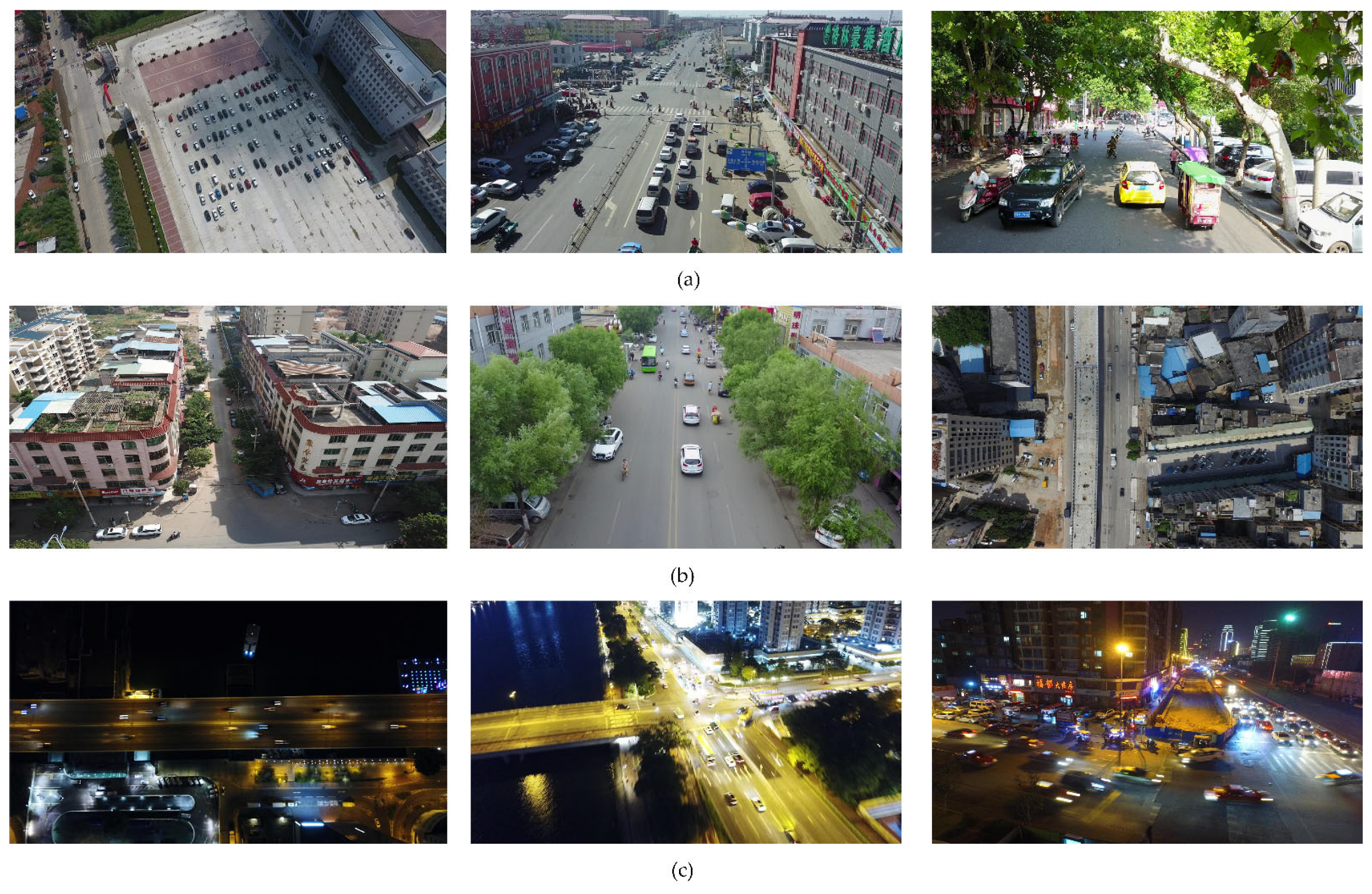
Examples for (a) object scale variations, (b) complex scenes, and (c) blurred images in UAV images.
Figure 1.
Examples for (a) object scale variations, (b) complex scenes, and (c) blurred images in UAV images.
Figure 2.
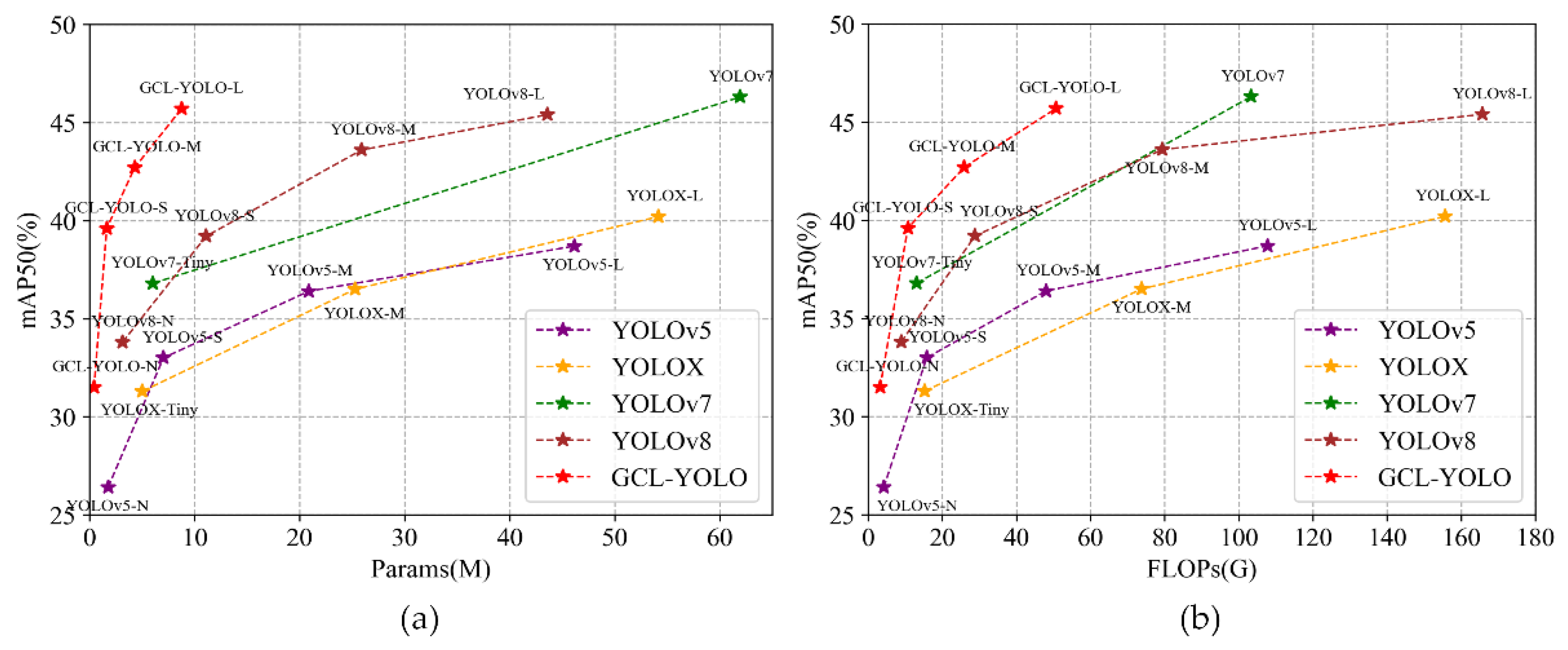
(a) Object detection accuracy versus parameter amount and (b) object detection accuracy versus calculation amount in different networks.
Figure 2.
(a) Object detection accuracy versus parameter amount and (b) object detection accuracy versus calculation amount in different networks.
Figure 3.
Structure of the GCL-YOLO network. The G-ELAG3 module represents a combined module of the G-Bneck2 module and the ELAG3 module. The backbone network outputs feature maps C2, C3, C4, and C5, whose number of channels are 128, 256, 512, and 512, respectively. The neck is an efficient layer aggregation and path aggregation network (ELA-PAN), whose inputs are four feature maps and outputs are three feature maps. The number of channels of three feature maps is 128, 256, and 512, respectively, and the downsampling rate is 4, 8, and 16, respectively. Note that the channel number of C5 is adjusted to 512 and is consistent with that of C4.
Figure 4.
Structure of the GhostConv module.
Figure 4.
Structure of the GhostConv module.
Figure 5.
Structure of the ghost bottleneck. (a) The G-Bneck1 with stride = 1 was used as a feature extraction layer and (b) the G-Bneck2 with stride = 2 was used as a downsampling layer. C denotes the number of channels; SiLU denotes the activation function; BN denotes the normalization; k denotes the convolution kernel size; Gap is the global maximum pooling; and σ is the sigmoid.
Figure 6.
Structures of (a) the ELAG3 and (b) the GSPPF.
Figure 6.
Structures of (a) the ELAG3 and (b) the GSPPF.
Figure 7.
Feature maps and heat maps of a UAV example image obtained with different sampling rates: (a) original image, (b) fine-grained feature map obtained with the sampling rate of 4, (c) fine-grained feature map obtained with the sampling rate of 32, (d) object detection result, (e) gradient-weighted class activation mapping (Grad-CAM) heat map obtained with the sampling rate of 4, and (f) Grad-CAM heat map obtained with the sampling rate of 32.
Figure 8.
Overlap between the predicted boxes and ground truth boxes.
Figure 8.
Overlap between the predicted boxes and ground truth boxes.
Figure 9.
(a) The label number of each object category and (b) the number of object labels of different sizes in the VisDrone-DET2021 dataset.
Figure 9.
(a) The label number of each object category and (b) the number of object labels of different sizes in the VisDrone-DET2021 dataset.
Figure 10.
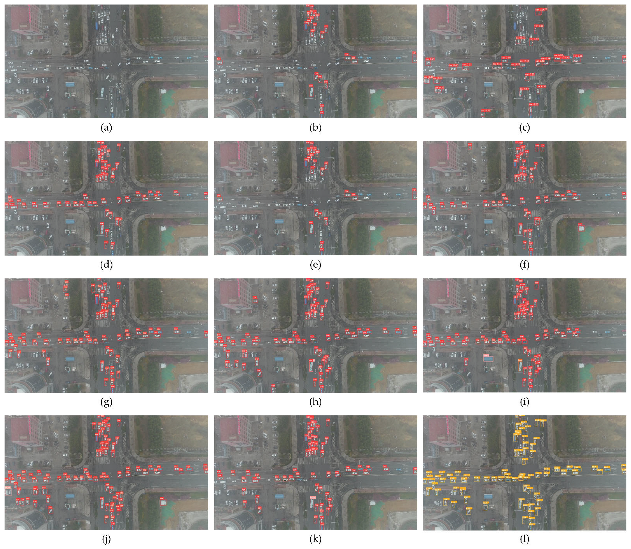
(a) Original image and local object detection results achieved by (b) YOLOv3-Tiny, (c) YOLOv4-Tiny, (d) YOLOv5-N (7.0), (e) YOLOv5-Lite-G, (f) Nanodet-Plus-M-1.5x, (g) YOLOX-Tiny, (h) YOLOv5-S (7.0), (i) PP-PicoDet-L, (j) YOLOv7-Tiny, (k) YOLOv8-S, and (l) GCL-YOLO-S.
Figure 10.
(a) Original image and local object detection results achieved by (b) YOLOv3-Tiny, (c) YOLOv4-Tiny, (d) YOLOv5-N (7.0), (e) YOLOv5-Lite-G, (f) Nanodet-Plus-M-1.5x, (g) YOLOX-Tiny, (h) YOLOv5-S (7.0), (i) PP-PicoDet-L, (j) YOLOv7-Tiny, (k) YOLOv8-S, and (l) GCL-YOLO-S.
Figure 11.
(a) Original image and local object detection results achieved by (b) YOLOv3-Tiny, (c) YOLOv4-Tiny, (d) YOLOv5-N (7.0), (e) YOLOv5-Lite-G, (f) Nanodet-Plus-M-1.5x, (g) YOLOX-Tiny, (h) YOLOv5-S (7.0), (i) PP-PicoDet-L, (j) YOLOv7-Tiny, (k) YOLOv8-S, and (l) GCL-YOLO-S.
Figure 11.
(a) Original image and local object detection results achieved by (b) YOLOv3-Tiny, (c) YOLOv4-Tiny, (d) YOLOv5-N (7.0), (e) YOLOv5-Lite-G, (f) Nanodet-Plus-M-1.5x, (g) YOLOX-Tiny, (h) YOLOv5-S (7.0), (i) PP-PicoDet-L, (j) YOLOv7-Tiny, (k) YOLOv8-S, and (l) GCL-YOLO-S.
Figure 12.
Comparisons between (a) the GCL-YOLO networks and (b) the YOLO networks.
Figure 12.
Comparisons between (a) the GCL-YOLO networks and (b) the YOLO networks.
Figure 13.
More detection results on the VisDrone2021 dataset. Different colored bounding boxes denote different object categories.
Figure 13.
More detection results on the VisDrone2021 dataset. Different colored bounding boxes denote different object categories.
Figure 14.
More detection results on the UAVDT dataset.
Figure 14.
More detection results on the UAVDT dataset.
Figure 15.
P–R curves obtained by (a) the YOLOv5-S network and (b) the GCL-YOLO-S network.
Figure 15.
P–R curves obtained by (a) the YOLOv5-S network and (b) the GCL-YOLO-S network.
Figure 16.
Confusion matrix obtained by the GCL-YOLO-S network with the IOU threshold of 0.45 and the confidence threshold of 0.25.
Figure 16.
Confusion matrix obtained by the GCL-YOLO-S network with the IOU threshold of 0.45 and the confidence threshold of 0.25.
Table 1.
Specifications of the different GCL-YOLO networks.
Table 1.
Specifications of the different GCL-YOLO networks.
| Network | α | β | Number of Feature Channels |
|---|
| GCL-YOLO-N | 0.33 | 0.25 | (32, 64, 128) |
| GCL-YOLO-S | 0.33 | 0.50 | (64, 128, 256) |
| GCL-YOLO-M | 0.67 | 0.75 | (96, 192, 384) |
| GCL-YOLO-L | 1.00 | 1.00 | (128, 256, 512) |
Table 2.
Parameter comparisons of different prediction heads.
Table 2.
Parameter comparisons of different prediction heads.
| Prediction Head | Downsampling Rate | Feature Map Size | Number of Channels | Parameters (MB) |
|---|
| P2, P3, P4, and P5 | 4×/8×/16×/32× | 160/80/40/20 | 128/256/512/1024 | 13.26 |
| P5 | 32× | 20 | 1024 | 9.97 |
| P2 | 4× | 160 | 128 | 0.17 |
Table 3.
Comparison between the GCL-YOLO network and the YOLOv5 network.
Table 3.
Comparison between the GCL-YOLO network and the YOLOv5 network.
| Network | Params(M) | GFLOPs | FPS | mAP50 (%) |
|---|
| YOLOv5-N | 1.77 | 4.2 | 68 | 26.4 |
| GCL-YOLO-N | 0.43 | 3.2 | 58 | 31.7 |
| YOLOv5-S | 7.04 | 15.8 | 60 | 32.7 |
| GCL-YOLO-S | 1.64 | 10.7 | 53 | 39.6 |
| YOLOv5-M | 20.89 | 48.0 | 57 | 36.4 |
| GCL-YOLO-M | 4.30 | 25.9 | 48 | 43.2 |
| YOLOv5-L | 46.15 | 107.8 | 53 | 38.7 |
| GCL-YOLO-L | 8.76 | 50.7 | 42 | 45.7 |
Table 4.
Comparisons between the GCL-YOLO-S network and the YOLOv5-S network.
Table 4.
Comparisons between the GCL-YOLO-S network and the YOLOv5-S network.
| Network | A1 | A2 | A3 | A4 | A5 | A6 | A7 | Params (M) | GFLOPs | FPS | mAP50 (%) | mAP50-95 (%) |
|---|
| YOLOv5-S | | | | | | | | 7.04 | 15.8 | 60 | 32.7 | 17.2 |
| | √ | | | | | | | 3.70 | 7.8 | 64 | 28.8 | 15.4 |
| GCL-YOLO-S | | √ | | | | | | 6.24 | 16.2 | 59 | 34.5 | 18.6 |
| | √ | √ | | | | | 4.18 | 11.1 | 55 | 32.9 | 17.4 |
| | √ | √ | √ | | | | 3.87 | 10.9 | 54 | 32.7 | 17.2 |
| | √ | √ | √ | √ | | | 3.97 | 12.7 | 50 | 37.2 | 20.2 |
| | √ | √ | √ | √ | √ | | 1.64 | 10.7 | 53 | 38.3 | 20.9 |
| | √ | √ | √ | √ | √ | √ | 1.64 | 10.7 | 53 | 39.6 | 21.5 |
Table 5.
Comparisons between the GCL-YOLO-S network and some lightweight networks on the VisDrone-DET2021 dataset.
Table 5.
Comparisons between the GCL-YOLO-S network and some lightweight networks on the VisDrone-DET2021 dataset.
| Network | Params (M) | GFLOPs | FPS | mAP50 (%) |
|---|
| All | Pedestrian | People | Bicycle | Car | Van | Truck | Tricycle | Awning Tricycle | Bus | Motor |
|---|
| YOLOv3-Tiny [10] | 8.68 | 12.9 | 86 | 15.9 | 19.4 | 18.4 | 3.2 | 49.9 | 12.7 | 9.7 | 8.2 | 4.0 | 14.6 | 18.9 |
| YOLOv4-Tiny [11] | 5.89 | 7.0 | 78 | 19.5 | 21.1 | 25.1 | 4.3 | 57.5 | 15.1 | 15.0 | 12.0 | 5.3 | 23.7 | 16.4 |
| YOLOv5-N | 1.77 | 4.2 | 68 | 26.4 | 33.1 | 27.1 | 6.9 | 67.8 | 23.5 | 18.4 | 12.9 | 9.1 | 32.0 | 31.3 |
| YOLOv5-Lite-G | 5.39 | 15.2 | 56 | 27.3 | 34.6 | 26.6 | 7.7 | 69.3 | 28.4 | 24.0 | 13.8 | 6.7 | 28.3 | 33.4 |
| Nanodet-Plus-M-1.5x | 2.44 | 3.0 | 78 | 30.4 | 27.9 | 24.1 | 7.4 | 73 | 35.1 | 27.8 | 17.9 | 8.4 | 49.3 | 33.3 |
| YOLOX-Tiny [12] | 5.04 | 15.3 | 70 | 31.3 | 35.8 | 21.9 | 9.6 | 73.3 | 34.7 | 28.1 | 18.1 | 10.2 | 46.3 | 34.9 |
| YOLOv5-S | 7.04 | 15.8 | 60 | 32.7 | 38.9 | 31.6 | 11.3 | 72.4 | 34.8 | 28.5 | 19.3 | 9.5 | 43.4 | 37.0 |
| PP-PicoDet-L [34] | 3.30 | 8.9 | 67 | 34.2 | 40.2 | 35.3 | 12.8 | 75.6 | 35.4 | 29.3 | 21.1 | 12.1 | 44.3 | 36.3 |
| YOLOv7-Tiny [14] | 6.03 | 13.1 | 51 | 36.8 | 41.5 | 38.3 | 11.9 | 77.3 | 38.9 | 29.1 | 23.4 | 11.7 | 48.6 | 47.1 |
| YOLOv8-S | 11.10 | 28.8 | 56 | 39.2 | 42.0 | 32.5 | 13.5 | 79.6 | 45.2 | 35.6 | 28.3 | 15.0 | 55.8 | 44.6 |
| GCL-YOLO-S | 1.64 | 10.7 | 53 | 39.6 | 48.0 | 37.6 | 15.7 | 81.1 | 42.5 | 32.7 | 26.4 | 12.4 | 53.8 | 46.0 |
Table 6.
Comparisons between the GCL-YOLO-S network and some lightweight networks on the UAVDT dataset.
Table 6.
Comparisons between the GCL-YOLO-S network and some lightweight networks on the UAVDT dataset.
| Network | Params (M) | GFLOPs | FPS | mAP50 (%) |
|---|
| All | Car | Truck | Bus |
|---|
| YOLOv3-Tiny [10] | 8.68 | 12.9 | 87 | 26.9 | 61.4 | 12.9 | 6.1 |
| YOLOv4-Tiny [11] | 5.89 | 7.0 | 77 | 27.7 | 63.5 | 13.4 | 6.4 |
| YOLOv5-N | 1.77 | 4.2 | 68 | 29.5 | 66.7 | 14.7 | 7.1 |
| YOLOv5-Lite-G | 5.30 | 15.1 | 58 | 27.6 | 65.2 | 12.7 | 4.8 |
| Nanodet-Plus-M-1.5x | 2.44 | 3.0 | 78 | 27.9 | 67.8 | 7.8 | 8.0 |
| YOLOX-Tiny [12] | 5.04 | 15.3 | 70 | 29.1 | 68.4 | 13.8 | 5.3 |
| YOLOv5-S | 7.04 | 15.8 | 62 | 29.8 | 70.1 | 14.4 | 5.0 |
| PP-PicoDet-L [34] | 3.30 | 8.9 | 67 | 31.1 | 71.2 | 16.5 | 5.8 |
| YOLOv7-Tiny [14] | 6.03 | 13.1 | 50 | 31.2 | 70.4 | 16.8 | 6.8 |
| YOLOv8-S | 11.10 | 28.8 | 57 | 31.9 | 71.3 | 17.4 | 7.1 |
| GCL-YOLO-S | 1.64 | 10.7 | 54 | 31.6 | 72.2 | 16.2 | 6.4 |
Table 7.
Comparisons between the GCL-YOLO-L network and some large-scale networks on the VisDrone-DET2021 dataset.
Table 7.
Comparisons between the GCL-YOLO-L network and some large-scale networks on the VisDrone-DET2021 dataset.
| Network | Input size | Params
(M) | GFLOPs | mAP50 (%) |
|---|
| All | Pedestrian | People | Bicycle | Car | Van | Truck | Tricycle | Awning Tricycle | Bus | Motor |
|---|
| TOOD [35] | 1333 × 800 | 31.81 | 144.40 | 41.0 | 41.5 | 31.9 | 19.2 | 81.4 | 46.5 | 39.6 | 31.8 | 14.1 | 53.5 | 50.5 |
| VFNet [36] | 1333 × 800 | 33.50 | 140.10 | 41.3 | 41.8 | 25.4 | 20.0 | 80.4 | 47.4 | 41.7 | 35.1 | 15.5 | 57.0 | 48.8 |
| Tridentnet [37] | 1333 × 800 | 32.85 | 822.19 | 43.3 | 54.9 | 29.5 | 20.1 | 81.4 | 47.7 | 41.4 | 34.5 | 15.8 | 58.8 | 48.9 |
| RSOD [19] | 608 × 608 | 63.72 | 84.21 | 43.3 | 46.8 | 36.8 | 17.1 | 81.8 | 49.8 | 39.3 | 32.3 | 19.3 | 61.2 | 48.6 |
| SlimYOLOv3 [22] | 832 × 832 | 20.80 | 122.00 | 45.9 | - | - | - | - | - | - | - | - | - | - |
| DMNet [20] | 640 × 640 | 41.53 | 194.18 | 47.6 | - | - | - | - | - | - | - | - | - | - |
| GCL-YOLO-L | 640 × 640 | 8.77 | 50.70 | 45.7 | 55.2 | 43.1 | 20.8 | 84.5 | 50.0 | 40.9 | 33.3 | 15.7 | 60.3 | 52.8 |


