Abstract
Crop leaf chlorophyll content (LCC) and fractional vegetation cover (FVC) are crucial indicators for assessing crop health, growth development, and maturity. In contrast to the traditional manual collection of crop trait parameters, unmanned aerial vehicle (UAV) technology rapidly generates LCC and FVC maps for breeding materials, facilitating prompt assessments of maturity information. This study addresses the following research questions: (1) Can image features based on pretrained deep learning networks and ensemble learning enhance the estimation of remote sensing LCC and FVC? (2) Can the proposed adaptive normal maturity detection (ANMD) algorithm effectively monitor maize maturity based on LCC and FVC maps? We conducted the following tasks: (1) Seven phases (tassel initiation to maturity) of maize canopy orthoimages and corresponding ground-truth data for LCC and six phases of FVC using UAVs were collected. (2) Three features, namely vegetation indices (VI), texture features (TF) based on Gray Level Co-occurrence Matrix, and deep features (DF), were evaluated for LCC and FVC estimation. Moreover, the potential of four single-machine learning models and three ensemble models for LCC and FVC estimation was evaluated. (3) The estimated LCC and FVC were combined with the proposed ANMD to monitor maize maturity. The research findings indicate that (1) image features extracted from pretrained deep learning networks more accurately describe crop canopy structure information, effectively eliminating saturation effects and enhancing LCC and FVC estimation accuracy. (2) Ensemble models outperform single-machine learning models in estimating LCC and FVC, providing greater precision. Remarkably, the stacking + DF strategy achieved optimal performance in estimating LCC (coefficient of determination (R2): 0.930; root mean square error (RMSE): 3.974; average absolute error (MAE): 3.096); and FVC (R2: 0.716; RMSE: 0.057; and MAE: 0.044). (3) The proposed ANMD algorithm combined with LCC and FVC maps can be used to effectively monitor maize maturity. Establishing the maturity threshold for LCC based on the wax ripening period (P5) and successfully applying it to the wax ripening-mature period (P5–P7) achieved high monitoring accuracy (overall accuracy (OA): 0.9625–0.9875; user’s accuracy: 0.9583–0.9933; and producer’s accuracy: 0.9634–1). Similarly, utilizing the ANMD algorithm with FVC also attained elevated monitoring accuracy during P5–P7 (OA: 0.9125–0.9750; UA: 0.878–0.9778; and PA: 0.9362–0.9934). This study offers robust insights for future agricultural production and breeding, offering valuable insights for the further exploration of crop monitoring technologies and methodologies.
1. Introduction
As one of the world’s top three major cereal crops, maize is extensively cultivated in various regions [1]. In agricultural production, crop maturity delineates the physiological stage of maturation, with maize maturity typically discerned through the assessment of indicators such as the milk line on maize kernels, moisture content, and leaf color. It serves as a pivotal determinant for yield formation and concurrently represents a crucial trait for assessing the growth stages of crops [2,3]. For agricultural decision makers, this parameter is a crucial indicator for selecting superior varieties [4]. Therefore, the precise monitoring of maize maturity is paramount for efficiently screening maize breeding materials and ensuring the security of grain production [5].
The chlorophyll content in maize leaves (LCC) typically exhibits specific dynamic changes, reflecting the turnover of photosynthetic activity and biochemical components [6]. The fractional vegetation cover (FVC) provides information about the spatial distribution of crop growth and effectively characterizes the growth status of maize [7,8]. As maize approaches maturity, photosynthesis slows, and nutrient transport decreases, reducing the demand for chlorophyll. Consequently, the LCC gradually decreases, causing the leaves to turn yellow. Simultaneously, vegetation begins to wither, causing a decrease in the density and coverage area of surface vegetation, i.e., a reduction in the FVC. Therefore, monitoring and analyzing these two parameters, LCC and FVC, effectively reflects the degree of maturity in maize.
Conventional field environments are typically chosen as observation sites for monitoring crop LCC, FVC, and maturity. However, traditional monitoring methods often involve intricate field surveys and manual sampling [9]. This approach is not only time-consuming and labor-intensive but also constrained by meteorological conditions and geographical location, making it challenging to generalize methods for regional monitoring [10]. Therefore, there is an urgent need to develop a monitoring method that is capable of rapidly and efficiently capturing information on the LCC, FVC, and maturity of field crops. In the past three decades, remote sensing technology has gained favor among researchers in crop monitoring [11]. In particular, unmanned aerial vehicle (UAV) remote sensing technology is preferred because of its low operational requirements and flexibility [12,13,14]. Based on these advantages, UAV remote sensing technology has been widely applied for monitoring crop phenotypic parameters, such as leaf area index (LAI), LCC, plant height, and biomass [15,16,17,18,19,20].
Numerous studies indicate that crop critical physiological and biochemical traits, such as leaf water content, LCC, and FVC, rapidly decrease with increasing maturity. Generally, crop physiological and biochemical trait parameter changes manifest as spectral responses [21]. For instance, a reduction in crop LCC may increase reflectance in the red-edge and near-infrared spectral bands. Therefore, maturity information can be extracted from crop canopy spectral reflectance. Significant progress has been made in remote sensing studies on extracting crop maturity information. In the field, spectral curve analysis based on time series vegetation index (VI) has become widely adopted. Although various algorithms, such as Fourier filtering [22] and asymmetric Gaussian functions [23], have been employed to smooth noise generated from long time series, they require complete vegetation index data for the entire growth period as input, introducing a notable degree of latency.
In addition to the method based on time series VI, several studies have underscored the potential of canopy spectral responses for inverting field crop parameters [11,24]. Subsequently, methods are employed to derive crop maturity information based on these crop parameters. This approach involves two main tasks: (1) estimating critical physiological and biochemical traits of crops (such as leaf water content, LCC, and FVC) based on remote sensing and (2) determining maturity information based on these critical physiological and biochemical traits of crops (such as leaf water content, LCC, and FVC).
For the first task, a common approach is to use VIs (such as the normalized difference vegetation index (NDVI) and greenness vegetation index (GVI)) in combination with models to establish relationships with crop parameters for estimating field crop parameters [25,26,27]. However, due to the significant differences in canopy structure among crops at different growth stages, traditional VIs contain limited feature information and struggle to comprehensively reflect the entire canopy structure of the crop growth period [28]. Additionally, VIs are insensitive to canopy changes under high crop cover conditions, often leading to underestimation of high values [29]. Researchers have introduced texture features (TF) based on VI images to address this issue and express crop canopy structure differences [28,30,31]. However, the number and contribution of shallow texture features extracted from VI images are limited [32]. In reality, the complexity of the field crop environment substantially exceeds the scope covered by these shallow textural features [33]. In other words, there is a need to extract richer textural features to enhance crop canopy structure information extraction. Many studies highlight the significant potential of deep learning in extracting deep features from images [34]. Therefore, extracting deep features (DF) from texture images using deep learning models has emerged as a viable approach to enhance the estimation of crop parameters. Typically, when VI or shallow texture features are used for crop parameter estimation, single-machine learning (ML) models, such as random forest (RF) or support vector machine (SVM) models, are often constructed [35]. However, single-ML models struggle to fully capture the complex relationships between measurements and features, leading to increased estimation bias, especially for increasingly smaller values. Ensemble learning algorithms integrate multiple machine learning models, providing stronger generalization and better resistance to overfitting, more effectively leveraging the advantages of model fusion [17,36].
For the second task, which involves determining maturity information based on critical physiological and biochemical traits of crops, the most common approach is the fixed threshold method. For example, some studies define maize grain maturity as a water content less than 35%, while sunflower fruit maturity is considered when the water content is greater than 40% [37,38]. Fiber fineness thresholds have also been employed to determine cotton maturity [39]. In addition to these threshold methods, machine learning technologies can be used to classify maturity via features such as the VI, LCC, and FVC. However, machine learning methods based on black-box rules cannot be used to comprehensively assess crop maturity. To address this issue, scholars have proposed monitoring soybean maturity based on crop parameter graphs combined with anomaly detection algorithms [40]. This method offers sufficient insights into soybean maturity through crop parameter monitoring. As a novel approach, whether this method can be applied to maize maturity monitoring has not been determined and warrants further exploration. Growth parameters combined with monitoring maize maturity is relatively scarce. These methodologies primarily involve the inversion of crop parameters, followed by their correlation with maturity information. For instance, some researchers collect UAV multispectral imagery and ground data, coupling radiative transfer and empirical models to invert maize grain moisture content, thereby monitoring maize maturity [41]. However, these relevant studies overlook the spatial variation of maize physiological and biochemical parameters (such as FVC and LCC) in the field, providing crucial information about maturity. In conclusion, the main focus of this study is to propose a high-precision maize FVC, LCC, and maturity information extraction model based on UAV remote sensing. This research is aimed at addressing the following questions: (1) Can image features extracted from pretrained deep learning networks and via ensemble learning enhance the estimation of remote sensing LCC and FVC data? (2) Can the proposed adaptive normal maturity detection algorithm (ANMD) applied to LCC and FVC maps be used to effectively monitor maize maturity? This study collected seven phases of maize canopy orthoimages and ground-truth data for LCC, FVC, and maturity information. The conducted work included (1) UAV data collection for seven phases (tassel initiation to maturity) of maize canopy orthoimages and corresponding ground-truth data for the LCC and six phases of the FVC. (2) Three features—VIs, TFs, and DFs—were tested for LCC and FVC estimation. Moreover, the potential of four single-machine learning models and three ensemble models for LCC and FVC estimation was evaluated. (3) The estimated LCC and FVC were combined with the proposed ANMD to monitor maize maturity.
2. Datasets
2.1. Study Area
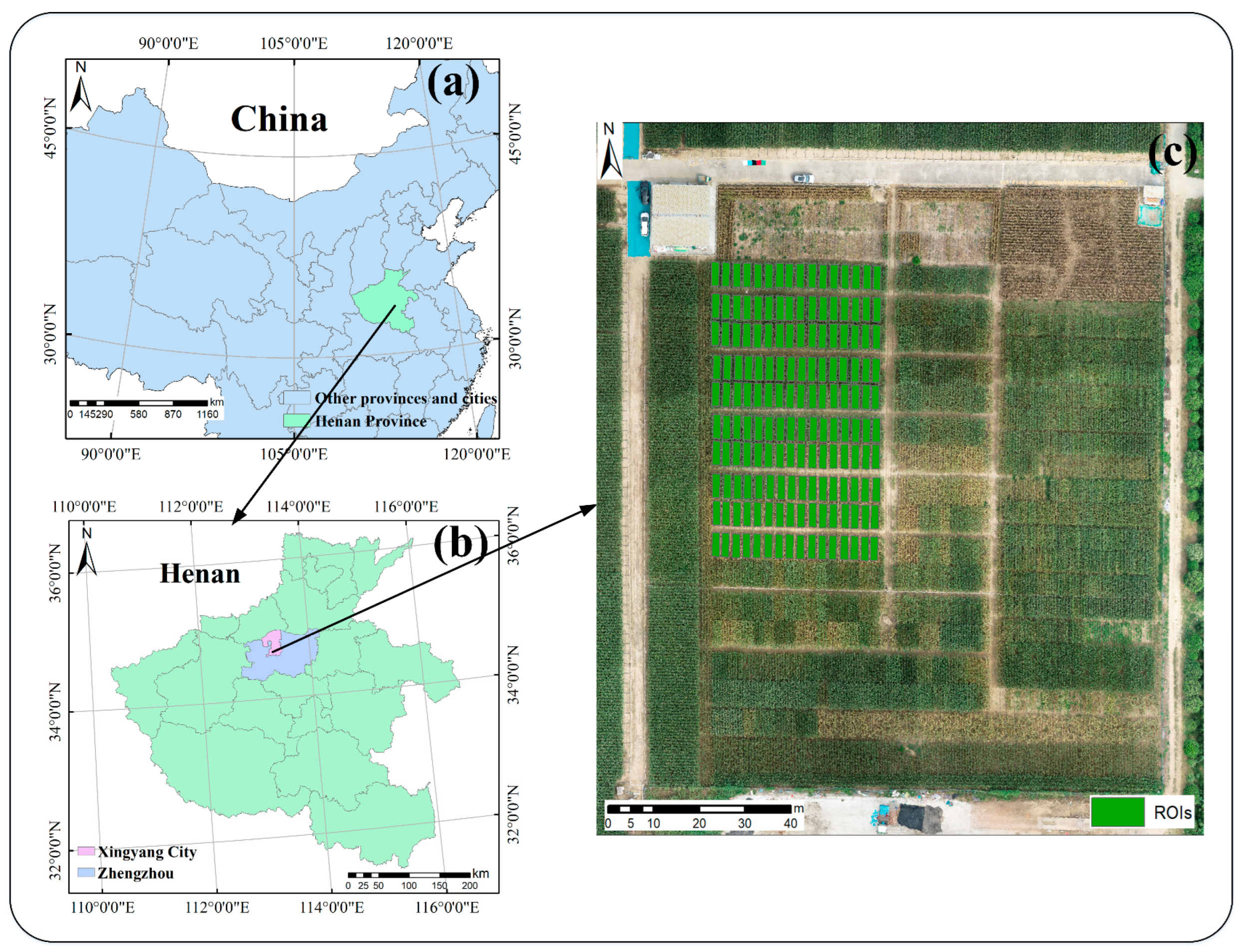
The research site is located in Xingyang city, Henan Province, China (Figure 1). Xingyang city is situated between 34°36′ and 34°59′N and between 113°7′ and 113°30′E [42]. Xingyang city experiences a warm, temperate, continental monsoon climate, with an average annual temperature of 14.8 °C and an average annual precipitation of 608.8 millimeters. The experimental site is dedicated to maize breeding and cultivates numerous varieties of maize. The experiment involved seven phases of data collection, which were conducted on the following dates in 2023: 27 July (tassel initiation stage, P1), 11 August (silking stage, P2), 18 August (blistering stage, P3), 1 September (milk ripening stage, P4), 7 September (waxy ripening stage, P5), 14 September (denting stage, P6), and 21 September (maturity stage, P7).

Figure 1.
(a) China; (b) Xingyang city, Henan Province; and (c) maize fields and sampling areas.
2.2. Field Experiments
2.2.1. LCC and FVC Acquisition
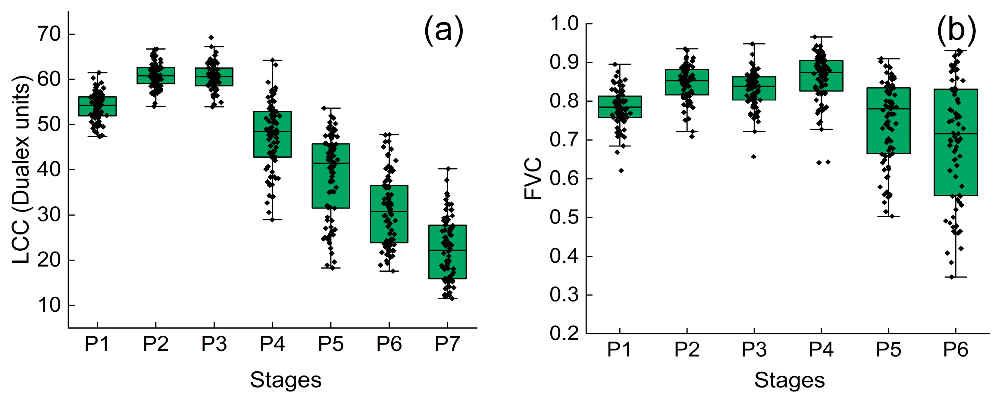
The LCC was measured using a portable SPAD-502 sensor (Soil and Plant Analyzer Development, Tokyo, Japan). The procedure involved selecting the first and second fully expanded leaves above the maize plants for measurement, considering both the tail and middle sections in the non-vein areas. These measurements were repeated three times at the center of each maize plot, and the mean was recorded as the final result. The results indicated that the maximum LCC occurred at P3, reaching 69.3 μg/cm2, while the minimum value was observed at P7, measuring 11.5 μg/cm2 (Table 1).

Table 1.
Field measurements of LCC and FVC.
The maize LAI was also measured using an LAI-2200C Plant Canopy Analyzer (LI-COR Biosciences, Lincoln, NE, USA). Prior to measurement, light intensity was measured in an open-backlight area. Subsequently, LAI measurements were obtained parallel and perpendicular to the maize rows. The LAI measurements were converted into the FVC using Equation (1). In this equation, G, ϴ, and Ω represent the spherical direction of the leaf projection factor, solar zenith angle, and clumping index (G = 0.5, ϴ = 0, and Ω = 1), respectively. Table 1 presents the analysis results of the maize field FVC dataset, revealing that the maximum FVC value at P4 was 0.966, while the minimum occurred at P6 with a value of 0.346.
2.2.2. UAV Imagery
In this study, the selected UAV model was the DJI Phantom 4 Multispectral Drone (DJI Technology Co., Ltd., ShenZhen, China), which has a visible light sensor and five single-band sensors (R, G, B, RedEdge, and NIR). Image acquisition occurred between 11:00 a.m. and 2:00 p.m. Before takeoff, the parameter settings were adjusted according to the experiment and experimental field environment. The flight altitude was approximately 30 meters, with a longitudinal overlap of approximately 80% and a lateral overlap of approximately 80%. After the images were acquired, DJI Terra software V4.0.1 version (DJI, Shenzhen) was used for high-precision stitching, generating digital orthophoto maps (DOM). Subsequently, the DOM samples underwent georeferencing and radiometric calibration processing. A vector map (Figure 1c) of the study area was created using ArcGIS (ArcGIS, ERSI, Inc., Redlands, CA, USA), and multispectral image information was extracted in batches using ENVI software 5.6.1 version (Exelis Visual Information Solutions, Boulder, CO, USA).
3. Methods
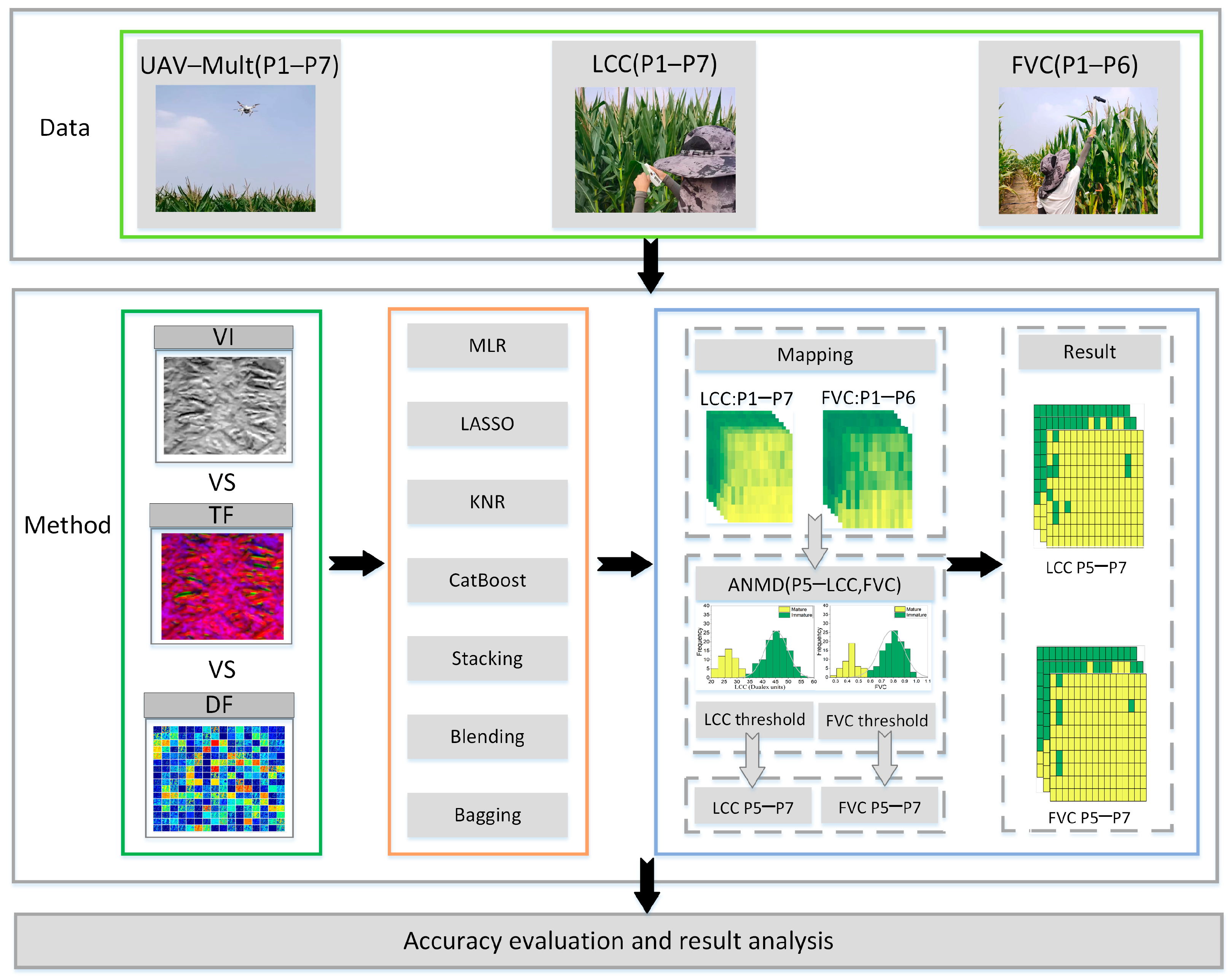
The specific steps of the technical workflow in this study (Figure 2) are outlined as follows:
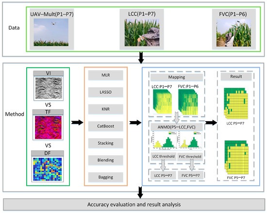
Figure 2.
Experimental technical workflow.
- Data Collection: At this stage, data collection was conducted, including obtaining data for seven phases of maize LCC, six phases of maize FVC, and seven phases of UAV-based maize multispectral DOMs.
- Feature Extraction: Feature extraction was performed based on vegetation index maps involving three key features: (a) VIs, (b) TFs based on Gray Level Co-occurrence Matrix (GLCM), and (c) DFs.
- Regression Model Construction: The three types of extracted features were input into preselected single-model regression models and ensemble models to estimate LCC and FVC.
- Maize maturity monitoring: Utilizing the ANMD, thresholds for LCC and FVC that correspond to mature maize at P5 were determined. These thresholds were subsequently applied during P5–P7 to monitor maize maturity.
3.1. Regression Techniques
Least absolute shrinkage and selection operator (LASSO) is a regularization method that is commonly utilized in linear regression [43]. Introducing an L1 regularization term, which is the sum of the absolute values of the parameters, into the loss function encourages the model coefficients to shrink toward zero. A unique feature of LASSO is that its regularization term induces sparsity in the model coefficients, automatically achieving feature selection by compressing the coefficients of features with minimal impact on the response variable to zero. LASSO has proven to be particularly powerful in handling high-dimensional data and feature selection.
Multiple linear regression (MLR) is a widely employed statistical and machine learning model for modeling the relationship between multiple independent variables and one dependent variable. Unlike simple linear regression, MLR considers the influence of multiple independent variables on the dependent variable, making it more suitable for reflecting complex relationships in the real world [44,45].
K-nearest neighbors regression (KNR) is a nonparametric regression method. The core idea of KNR is to predict the target variable by considering the k-nearest neighbors’ response variables to the predicted data point. During the prediction process, the mean or weighted mean is used to estimate the value of the target variable. KNR is suitable for handling complex nonlinear relationships, as it makes no strong assumptions about the model form, providing flexibility.
CatBoost is a machine learning framework based on gradient boosting trees that is known for its efficient handling of categorical features without the need for one-hot encoding or label encoding. Employing a rank-based algorithm improves the training speed and performance of the model. CatBoost regression effectively handles missing values without requiring additional preprocessing [46].
Ensemble learning integrates the predictions of multiple base models to construct a meta-model, enhancing overall performance. Unlike individual models, ensemble learning frameworks leverage the strengths of different models, improving generalization and mitigating overfitting to some extent [47,48]. The authors divided the original models into meta-models and base models for combined regression. Different ensemble models have different operating mechanisms. However, whether through voting or weighting, they operate based on the collaboration of multiple models. Even in scenarios with large datasets and limited computational resources, ensemble models can enhance overall performance by synthesizing the advantages of different base models. Here, we select several commonly used ensemble model frameworks, including stacking, blending, and bagging ensemble learning.
3.2. Adaptive Normal Maturity Detection Algorithm
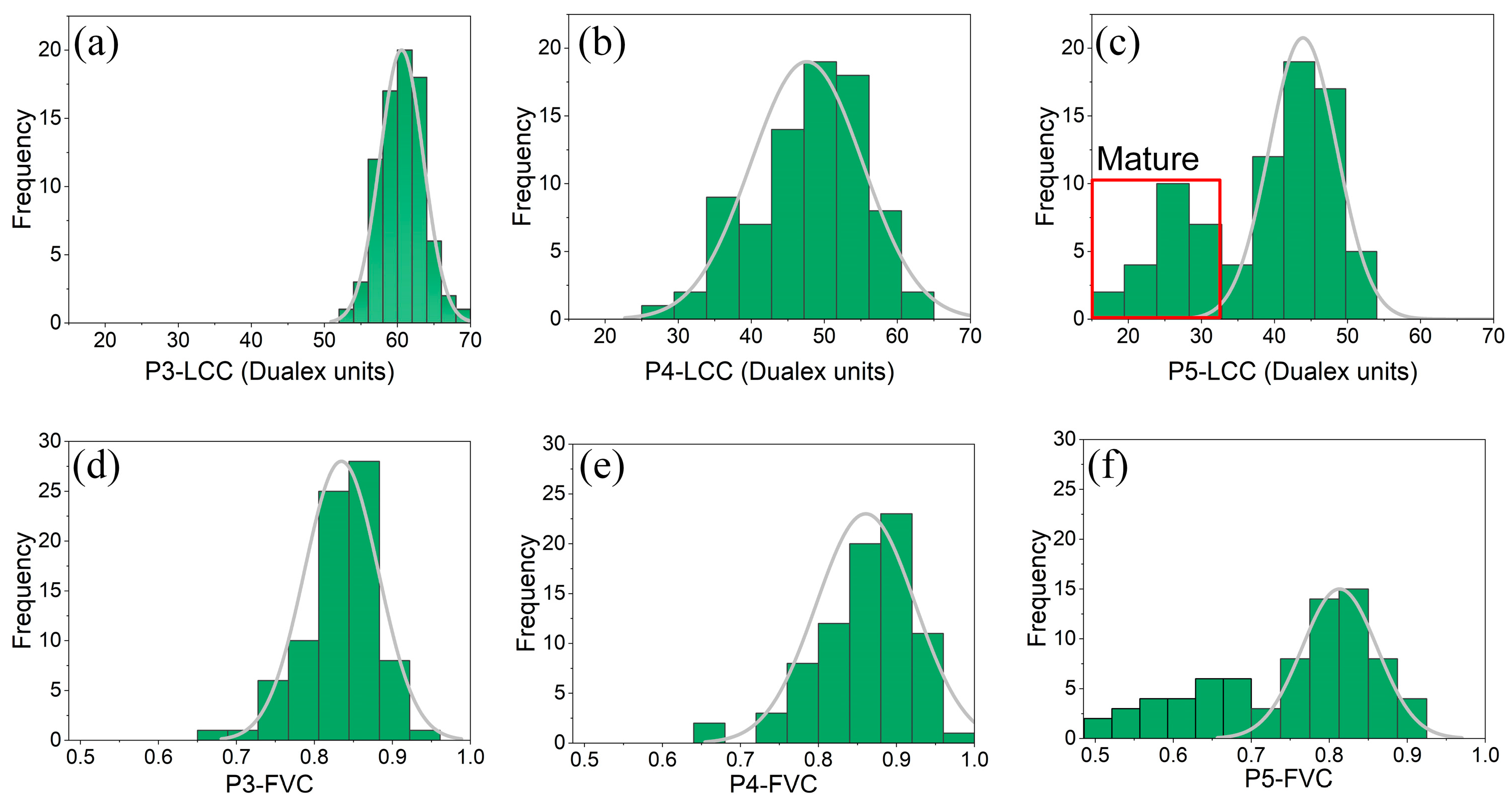
Figure 3 shows the grayscale histograms of ground-measured LCC and FVC during P3, P4, and P5. In P3 and P4, when the maize plants were immature, the ground-measured LCC and FVC exhibited a normal distribution. However, during P5, the expression of early-maturing traits in the maize varieties led to differences in the distributions of LCC and FVC. The LCC and FVC of most immature maize plots fall within the high-value range and follow a normal distribution. In contrast, the mature maize in specific zones showed a trend toward low values, deviating from the original normal distribution. Therefore, based on these characteristics, we propose the ANMD algorithm for monitoring maize maturation.
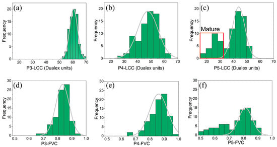
Figure 3.
Histograms of LCC and FVC (a) P3-LCC; (b) P4-LCC; (c) P5-LCC; (d) P3-FVC; (e) P4-FVC; (f) P5-FVC.
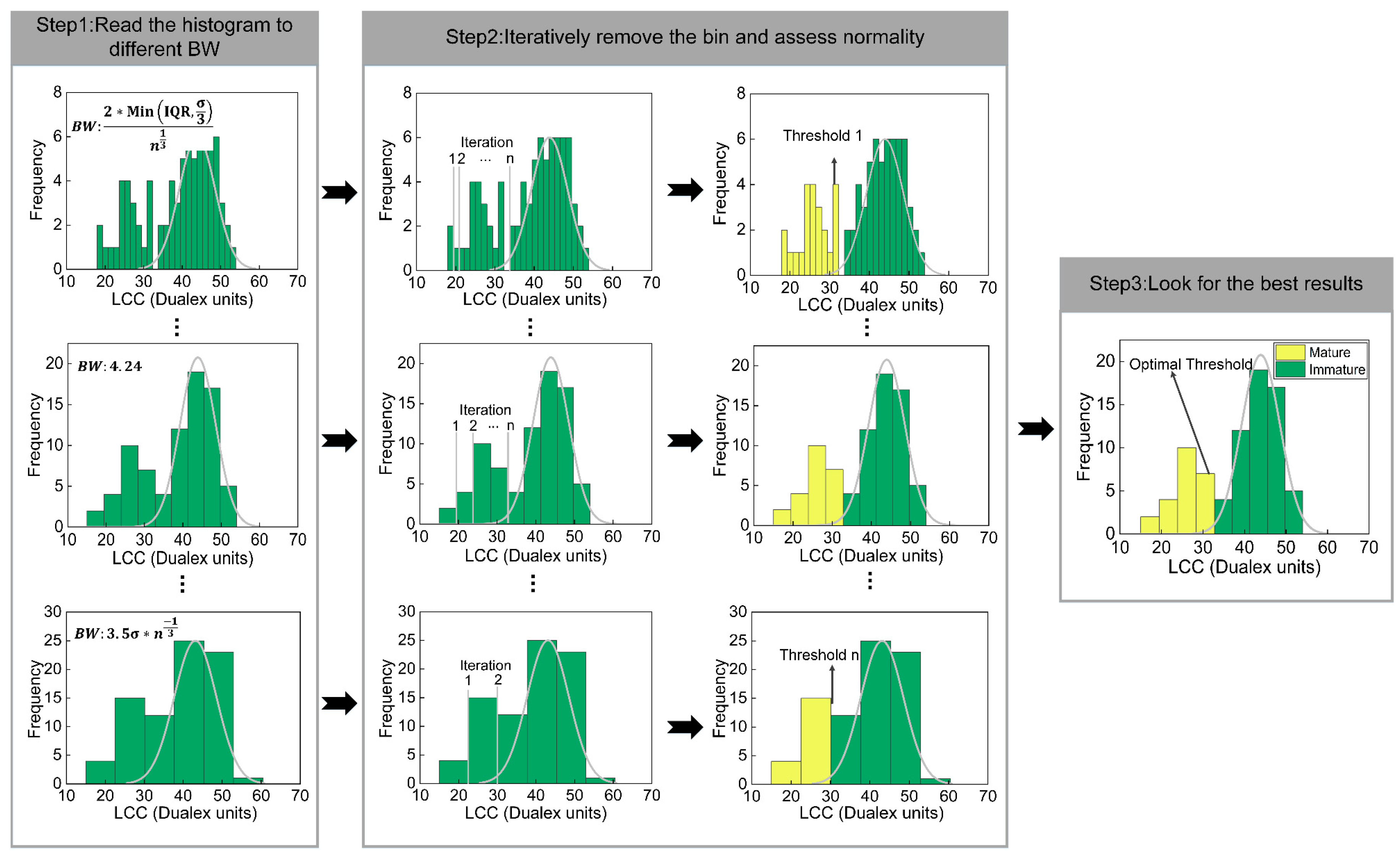
Below, we illustrate this technique using the example of monitoring maturity based on the LCC measurements obtained at P5 (Figure 4). (1) The algorithm starts by reading the ground-measured LCC for maize and presenting it on a statistical distribution histogram. Different bin widths (BWs) yield different frequency distribution histograms. Therefore, the algorithm explores various BWs to obtain the optimal distribution. Considering the convergence performance of the algorithm, we define the range of BWs using the Freedman–Diaconis and Scott rules [49]. (2) Each histogram exhibits different kurtosis and skewness values, which are crucial measures of histogram normality. Therefore, we use the combination of kurtosis and skewness as the evaluation criterion for normality. The combination that reaches the minimum absolute value is considered the most normal distribution. Groups deviating from a normal distribution were considered distant from the median and distributed at the tails of the histogram. Iterative removal of tail values was performed to approach the most normal distribution, and corresponding thresholds were recorded. This process is repeated for different BWs. (3) The algorithm seeks the optimal threshold corresponding to the “most normal distribution”, which serves as the decision value for determining whether the maize is mature.
where IQR is the interquartile range of the sample, σ is the standard deviation, and n is the number of input samples.

Figure 4.
Principle of the adaptive normal anomaly detection algorithm (ANMD).
3.3. Feature Extraction
3.3.1. Vegetation Indices
Physiological parameters, such as leaf water content and color in the crop canopy, undergo dynamic changes at different growth stages. Due to these characteristics, the canopy reflectance of crops varies across different growth stages. Individual band information contains limited detail, and the establishment of VIs effectively integrates spectral information [50]. Therefore, it is possible to characterize vegetation information based on the differences in these band combinations. This study selected eight widely used VIs from a pool of 49 VIs for estimating LCC and FVC. The specific selections are outlined in Table 2.

Table 2.
Vegetation indices.
3.3.2. GLCM Texture Features
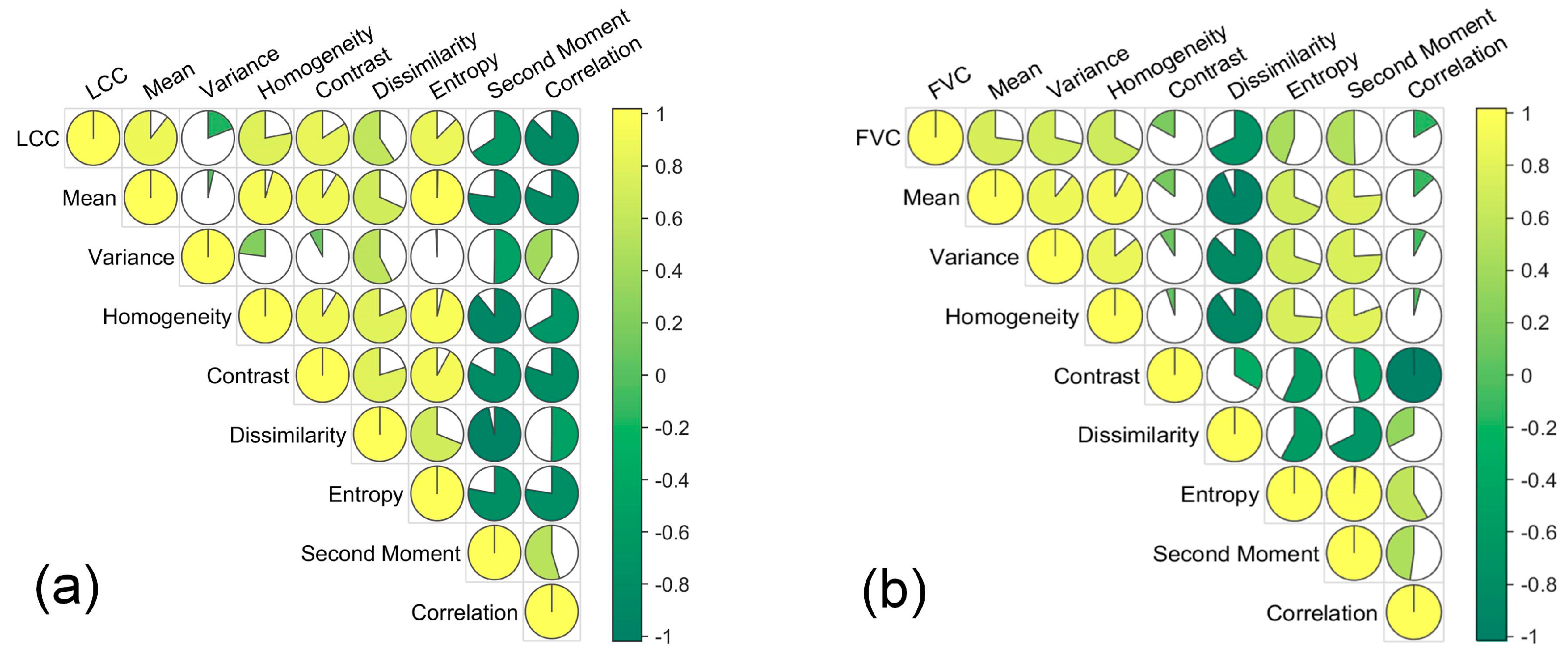
Image TFs can slightly characterize the canopy structure of crops. In this study, we extracted eight texture features based on GLCM, including mean, variance, homogeneity, contrast, dissimilarity, entropy, second moment, and correlation. The mean represents the regularity of the texture information in remote sensing images; variance measures the average contrast in the image, with smaller values indicating a more uniform distribution of pixel values; homogeneity reflects the uniformity of local grayscale in the image; contrast represents the depth of furrows and wrinkles in the image; dissimilarity measures image dissimilarity; entropy quantifies the randomness of the image; second moment indicates the image’s moments; and correlation assesses the image’s correlation. Considering the maize planting environment and the pixel size of the UAV images, we used a window size of 3 × 3 to extract the TF. For detailed information on the TFs, please refer to Table 3.

Table 3.
Texture features.
3.3.3. Deep Features
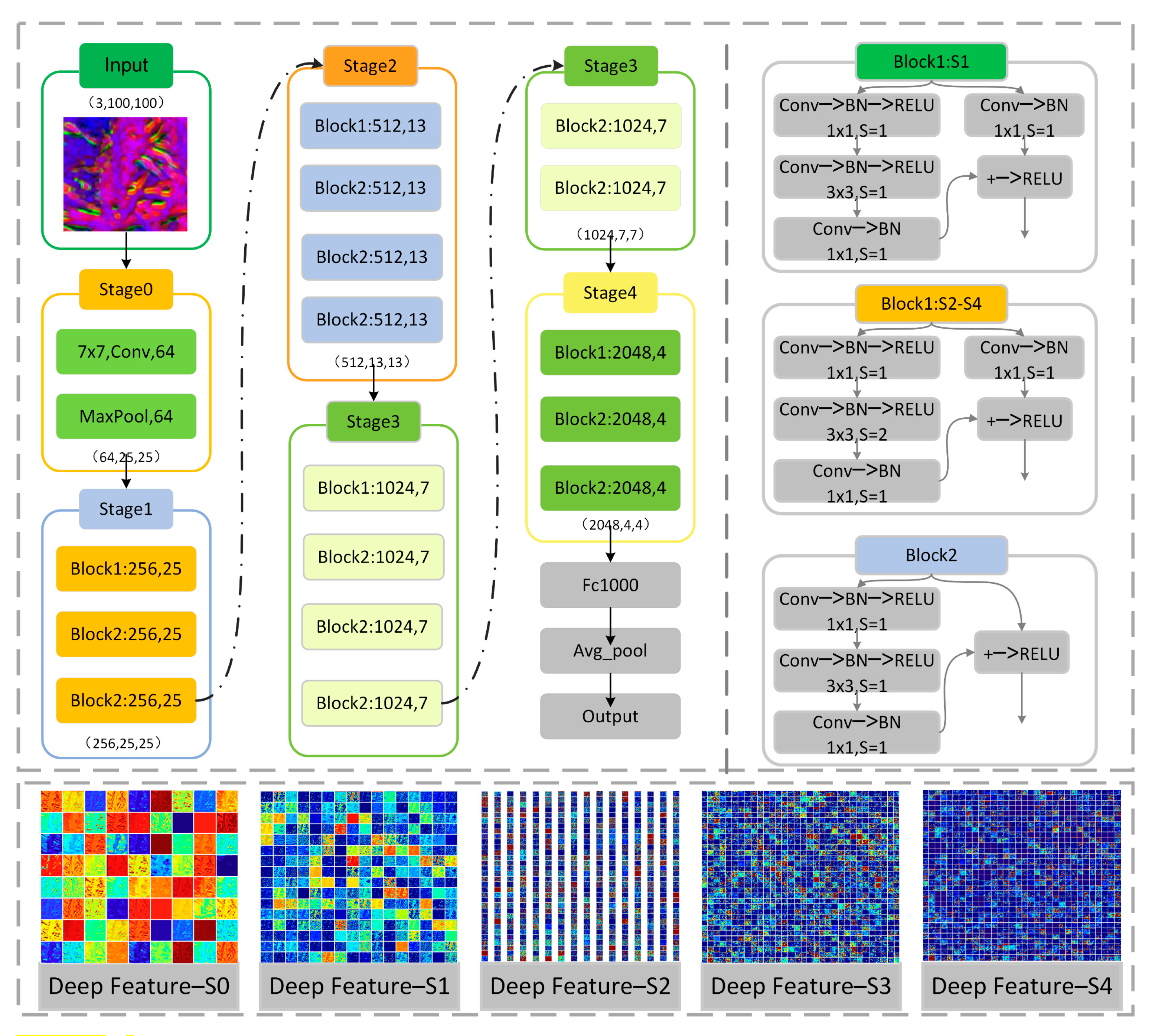
ResNet50 successfully addresses the vanishing and exploding gradient issues during deep neural network training by introducing an innovative residual connection structure. The ResNet50 architecture incorporates multiple convolutional layers to extract information at various scales. The computational operations performed by these convolutional layers effectively model spatial relationships within the images, allowing ResNet50 to discern different levels of detail in agricultural land cover. Consequently, it excels in capturing deep features related to crop surface coverage with enhanced proficiency [58]. These deep features mitigate the estimation errors caused by the complex canopy structure of the environment and crops. Therefore, ResNet50 has significant potential for accurately estimating LCC and FVC. ResNet50 extracts transformed features through five stages. The input stage uses the selected texture feature maps as input to the model. Stage 0 to Stage 4 (S0–S4) transform the original feature tensor through different transformations. In these stages, we obtain DFs with dimensions of 64, 256, 512, 1024, and 2048 (Figure 5).
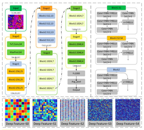
Figure 5.
Process of deep feature extraction.
3.4. Performance Evaluation
To assess the accuracy of the LCC and FVC estimates, this study employed the coefficient of determination (R2), root mean square error (RMSE), and average absolute error (MAE) as evaluation metrics.
where, represents the actual measured values, denotes the estimated mean, and n represents the number of samples. A model is considered more accurate for identical sample data if it exhibits higher coefficients of determination and lower root mean square error values.
Regarding the precision of maize maturity monitoring, a comparative analysis contrasts the surveyed maize maturity data by ground-based professional breeders with the predicted maturity data. Subsequently, the accuracy is computed by incorporating a confusion matrix. Three key metrics, namely, overall accuracy (OA), producer accuracy (PA), and user accuracy (UA), are selected to assess maturity monitoring accuracy (Table 4). OA quantifies the model’s capability to detect instances across all categories accurately. UA refers explicitly to the model’s ability to identify mature or immature corn regions correctly. PA pertains to the proportion of accurately matched instances to the ground truth within all monitored categories.

Table 4.
Confusion matrix.
In this context, we define true positives (TP) as cases where the actual and predicted values are mature. Similarly, true negatives (TN) are instances where the actual value and predicted value are also immature. The definitions apply to other scenarios. FN represents instances where the true condition is maturity, but the prediction erroneously indicates immaturity. FP denotes instances where the true condition is immaturity, but the prediction incorrectly suggests maturity.
4. Results
4.1. Statistical Analysis of LCC and FVC
We constructed box plots to better understand the dynamic variations in LCC and FVC in maize across different growth stages (Figure 6). The results indicate a consistent increase in maize LCC from stages P1 to P3, followed by a gradual decrease from stages P4 to P7 (Figure 6a). In contrast, the maize FVC exhibited a distinct pattern, with a noticeable decrease occurring only at stage P5 (Figure 6b). This discrepancy is attributed to the notion that even though the maize LCC decreases at stage P4, the maize has not yet matured. In other words, this decrease may be related solely to changes in leaf color, with minimal variation in leaf area. Overall, due to the specific characteristics of the breeding field, both LCC and FVC tended to increase during the early growth stages. As the expression of early maturity traits unfolds in the subsequent stages, significant differences in LCC and FVC become evident.
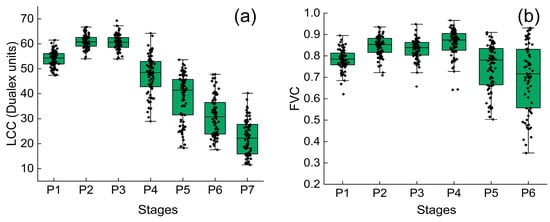
Figure 6.
(a) Overall trend of ground LCC; (b) overall trend of ground FVC.
4.2. Feature Correlation Analysis
4.2.1. Correlation Analysis of the Vegetation Indices
To better understand the relationship between LCC or FVC and VI, we conducted a correlation (r) analysis (Figure 7). The results revealed negative correlations between LCC and OSAVI and VARI and positive correlations with the remaining indices. Notably, LCC exhibited the highest correlation with NDRE (0.904), while the correlation was lowest with VARI (−0.537) (Figure 7a). On the other hand, FVC demonstrated positive correlations with most VIs (excluding the GNDVI and VARI). Specifically, the FVC had a greater correlation with OSAVI (0.730) and a lower correlation with the MTCI (0.415). Consequently, we selected the NDRE and OSAVI as the VIs for estimating LCC and FVC, respectively.
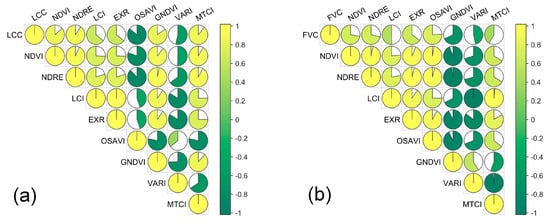
Figure 7.
Correlation analysis of the vegetation indices (a) LCC and (b) FVC.
4.2.2. Correlation Analysis of GLCM Texture Features
We constructed the TFs of the NDRE and OSAVI images based on the correlations between the VIs. Subsequently, a correlation analysis was conducted. The results indicated (Figure 8) that the correlations of LCC and FVC with the eight GLCM TFs tended to be in the range of [−0.871, −0.892] and [−0.679, 0.729], respectively. Notably, LCC exhibited greater correlations with the mean (0.892), entropy (0.872), and correlation (−0.871) (Figure 8a). Consequently, we opted to use the overlay of these three GLCM texture feature maps as input for the ResNet50 model for LCC. Similarly, FVC had stronger correlations with the mean (0.729), variance (0.712), and homogeneity (0.672) (Figure 8b).
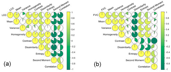
Figure 8.
GLCM texture feature correlation analysis for (a) LCC and (b) FVC.
4.2.3. Correlation Analysis of Deep Features
We obtained a substantial number of deep features transformed by ResNet50. Specifically, the extracted features were converted into a one-dimensional array, resulting in 2048×4×4 features. Subsequently, correlation analysis was conducted, and correlation plots were generated between the deep features and LCC and FVC (Figure 9 displays only a subset of representative samples due to the abundance of deep features). The results indicate that the extracted features exhibit a maximum positive correlation with LCC at 0.950, and the maximum absolute negative correlation is −0.907 (Figure 9a). Compared to those of VI and TF, |r| increased by approximately 0.045. For FVC, the highest positive correlation with features was 0.759, and the highest absolute negative correlation was −0.717 (Figure 9b). Compared to those of VI and TF, |r| increased by approximately 0.030. This finding suggested that the features obtained after ResNet50 processing may have a stronger association with LCC and FVC.

Figure 9.
Correlation analysis of deep features for (a) LCC and (b) FVC.
4.3. LCC and FVC Estimation and Mapping
4.3.1. LCC and FVC Estimation
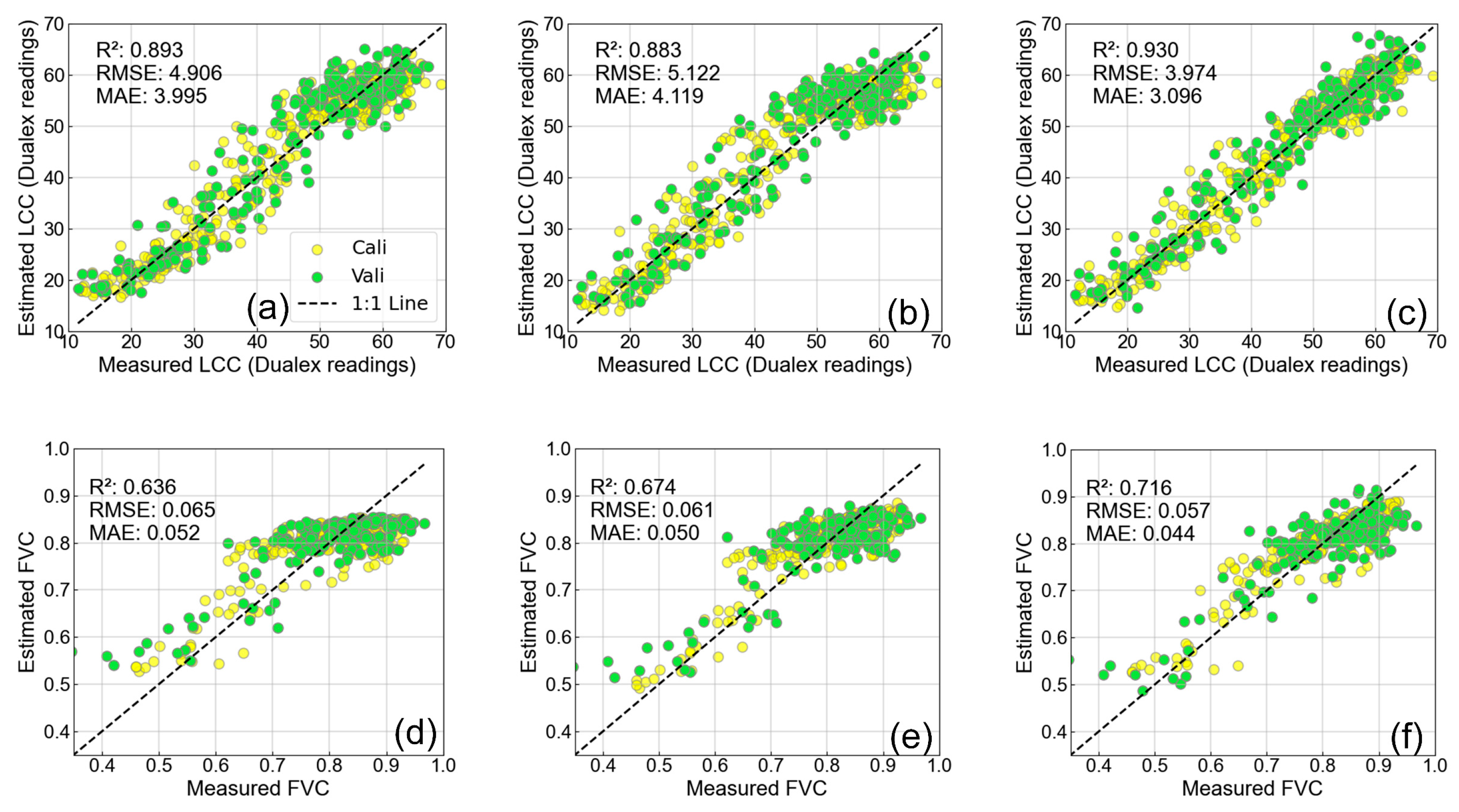
Before estimation, we partitioned the data into a training set (336 samples) and a test set (224 samples) in a 6:4 ratio. Subsequently, the selected 1 VI, 3 TFs, and 2048×4×4 DFs were individually input into four single and three ensemble models to estimate LCC and FVC. Table 5 presents the results of LCC estimation using 21 different strategies. The overall performance of LCC estimation appears favorable (R2: 0.790–0.930; RMSE: 3.974–6.861; and MAE: 3.096–5.634). With different feature inputs, we investigated the impact of individual models and ensemble models on the estimation results. When the VI was used as the input, stacking performed the best (R2: 0.893; RMSE: 4.906; and MAE: 3.995); when TF was used as the input, blending achieved the highest estimation accuracy (R2: 0.883; RMSE: 5.122; and MAE: 4.119); and when DF was used as the input, stacking showed the best performance (R2: 0.930; RMSE: 3.974; and MAE: 3.096). The scatter plots for these three strategies (Figure 10) also indicate that DF+ stacking has superior estimation performance.

Table 5.
LCC estimation results.
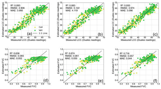
Figure 10.
Scatter plot: (a) Estimation of LCC using stacking + VI; (b) blending + TF estimation of LCC; (c) stacking + DF estimation of LCC; (d) blending + VI estimation of FVC; (e) blending + TF estimation of FVC; and (f) Stacking + DF estimation of FVC.
Similarly, the results of FVC estimation (Table 6) indicate that the ensemble models demonstrate higher accuracy across the three features. When the VI is used as the input, blending yields the best performance, with an R2 of 0.636, an RMSE of 0.065, and an MAE of 0.052. When TF is used as the input, blending also performs well, with an R2 of 0.674, an RMSE of 0.061, and an MAE of 0.050. Moreover, when DF is used as an input, the stacking model exhibits the best performance (R2: 0.716; RMSE: 0.057; and MAE: 0.044).

Table 6.
FVC estimation results.
We visualized the estimation results in scatter plots, as shown in Figure 10. When the DF is selected as the feature for estimating LCC, the overall predicted values are closer to the 1:1 line, indicating higher estimation accuracy. However, a saturation effect occurs when VIs and TFs are used as features for estimating FVC. Interestingly, the use of DF mitigates this saturation effect. This observation suggested that, similar to LAI estimation, FVC estimation is prone to saturation effects.
4.3.2. LCC and FVC Mapping
We opted for the best-performing strategy (DF + stacking) to generate LCC and FVC maps for stages P1–P7. As depicted in Figure 11, the LCC gradually increases from stages P1 to P3 and then decreases from stages P4 to P7. The FVC plateaued at P4, initiating a decrease. Due to the characteristic parameters of crops, the changes in LCC during the same period are more pronounced than those in FVC. These results align with the ground-based measurements and analyses presented in Figure 6.
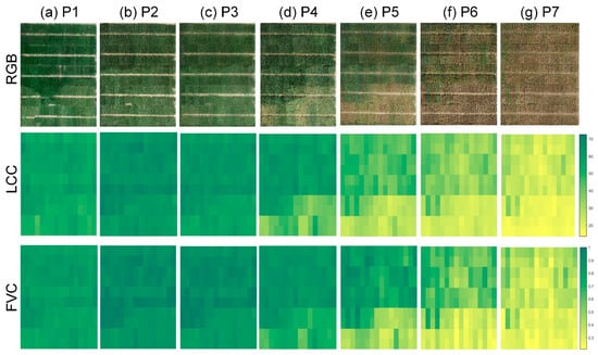
Figure 11.
LCC and FVC estimation maps: (a–g) represent P1–P7, respectively. First line: RGB image; second line: LCC mapping; and third line: FVC drawing.
4.4. Maize Maturity Monitoring
Based on the analysis of LCC and FVC for stages P3 to P5, we applied the ANMD algorithm to the data for P5. The results (Figure 12) depict that the yellow area (early-maturing maize varieties) deviates from a normal distribution. In contrast, the green area (regular varieties) demonstrated a normal distribution, consistent with ground-based analyses. In this case, we obtained the threshold values corresponding to LCC and FVC for P5 as 32.865 and 0.572, respectively.
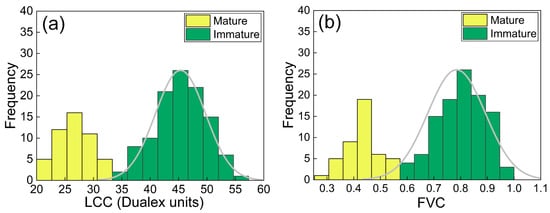
Figure 12.
LCC, FVC threshold calculation: (a) LCC and (b) FVC.
Utilizing the obtained thresholds for maturity monitoring during P5 yielded high OA (LCC: 0.9875; FVC: 0.9750). Consequently, we applied the P5 thresholds to subsequent periods. The results indicated that the monitoring OA ranged from 0.9625 to 0.9812, whereas for FVC monitoring during the same period, the overall accuracy ranged from 0.9125 to 0.9688. These findings suggested that our proposed method for monitoring maize maturity demonstrated excellent performance. The detailed monitoring results are provided in Table 7.

Table 7.
Mature monitoring accuracy.
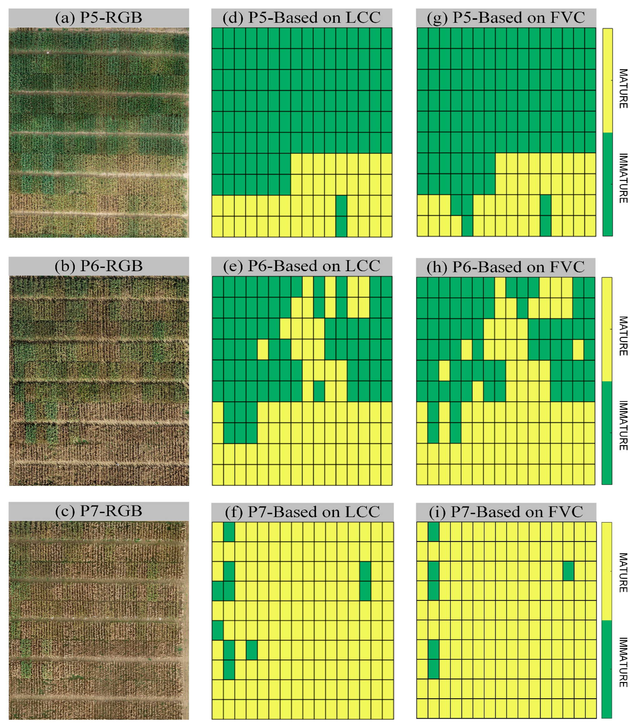
Following the results evaluation, we visualized the outcomes in the sampling area (Figure 13). Observations reveal that during P5, there are fewer mature areas. However, by P6, the distribution of mature areas becomes more diverse. By P7, the entire region generally exhibited maturity. Additionally, note that during the same period, the maturity monitoring outcomes based on LCC and FVC slightly differed. Overall, our monitoring approach demonstrated an effective performance across different periods.
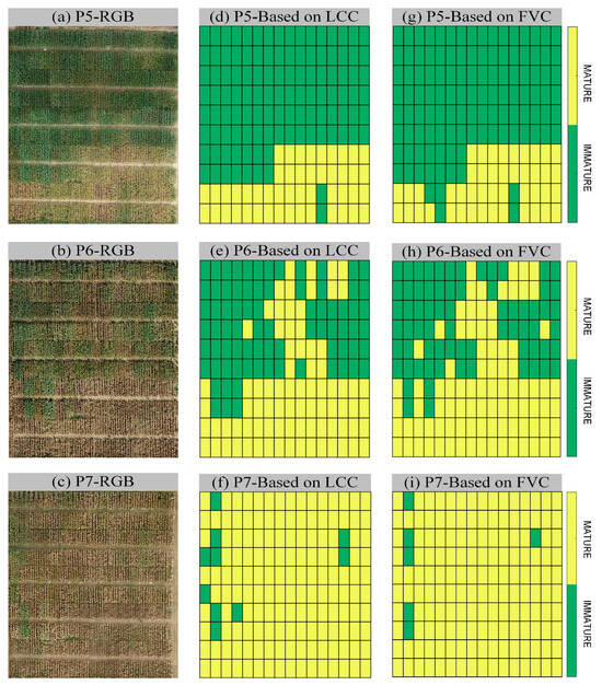
Figure 13.
Mature mapping of the sampling areas.
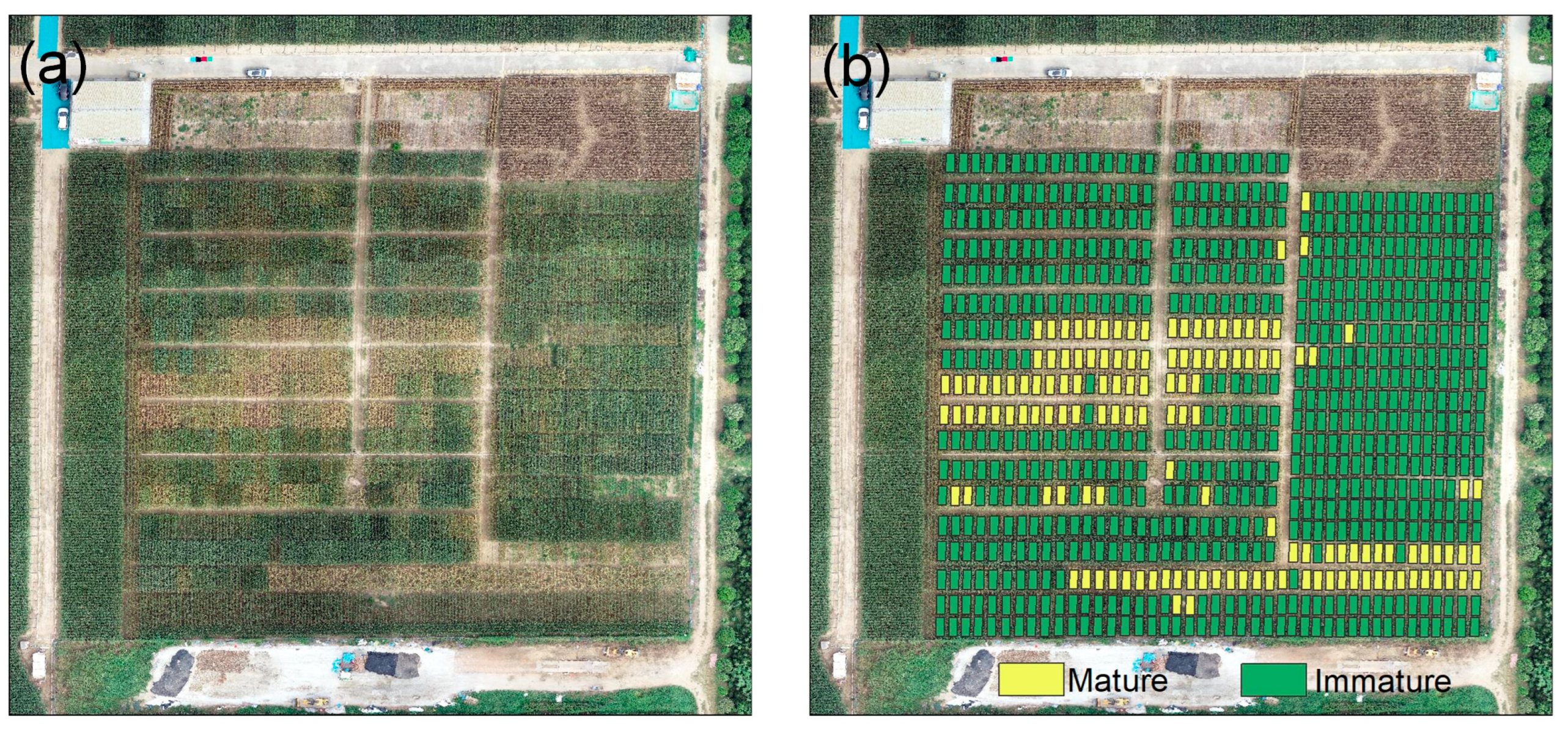
To acquire comprehensive maturity information for the entire field area, we generated a maturity map for the entire region (Figure 14). Using P5 as an example, we applied the maturity threshold derived from the P5 maize LCC to all plots (a total of 780) and created an overall map. The visual representation of the mapping results aligns with the visual appearance of the bottom-left base map (Figure 14a).

Figure 14.
Mapping of field maturity during P5. (a) RGB image of experimental field; (b) Maturity image of experimental field.
5. Discussion
5.1. Impact of Different Features and Models on LCC and FVC Estimation
The estimation of crop parameters based on empirical methods has long been favored by researchers, with VI being the most common “feature” used for estimation. However, the effectiveness of VI monitoring for crop parameter estimation is often compromised in complex agricultural environments [59]. Additionally, inherent characteristics of crop parameters, such as the LAI and FVC, can lead to saturation or reduced estimation capabilities. To address this issue, scholars have introduced TF to mitigate the saturation phenomenon [60]. When crops reach a high canopy cover, the changes in canopy structure are not as pronounced as those in the early growth stages over a considerable period [61,62]. Shallow texture features may not effectively capture such changes. Our experimental results also demonstrated this trend (Figure 10). Numerous studies indicate that deep learning can better explore the latent deep features in images. However, most studies tend to investigate the combined effects of deep learning models with original data imagery for estimating crop parameters [40,61,63,64,65,66]. Overlooking the contribution of the deep information contained in texture images. Our research results suggest promising prospects for exploring stable features in crop parameter estimation using DFs derived from GLCM texture maps (Figure 10c,f).
This approach also introduces several challenges: (1) faced with complex and diverse features, a more powerful estimation model may be needed; and (2) even under the same spatiotemporal conditions, the LCC and FVC of the same crop may exhibit heterogeneity. Therefore, ensuring that a given model performs well in estimating both parameters is challenging. When using vegetation indices (VIs) as features for estimating LCC, the estimation performance of CatBoost was shown to be superior to that of Lasso. This finding indicates that nonlinearity dominates the relationship between VIs and LCC. In reality, most relationships between crop parameters and canopy features exhibit both linear and nonlinear relationships [40]. This finding implies that a single model may not be fully effective at fitting complex agricultural data. In contrast, ensemble models can effectively integrate single models using a hierarchical structure, reducing the risk of overfitting, mitigating the impact of data biases, and improving predictive capabilities [67,68]. This outcome was also evident in our experiments. Using LCC estimation as an example, the ensemble models demonstrated better performance regardless of which feature was utilized as the input (stacking + VI; blending + TF; and stacking + DF). Additionally, we found that bagging, as an ensemble model, did not consistently maintain good estimation performance, which may be related to Bagging’s use of average weighting, which is susceptible to the influence of outliers or extreme values.
5.2. Monitoring and Analysis of Maize Maturity
Previous research has indicated that leaf color and the degree of leaf shedding are crucial indicators for monitoring crop maturity [69]. Compared to assessing crop maturity based solely on VI, evaluating crop maturity based on crop LCC and FVC with distinct physical significance is more convincing and interpretable. Maize plots that mature prematurely in the study area disrupt the established balance and act as “outliers”. This novel approach has been applied in soybean breeding material selection but has not been attempted in maize experimental fields. Additionally, whether multispectral imagery can be combined with this method still needs to be determined. Therefore, this study is aimed at further exploring and analyzing this issue. We conducted maturity monitoring during P5, which achieved high monitoring accuracy (OA based on LCC monitoring: 0.9875; OA based on FVC monitoring: 0.9750). Furthermore, we extended the obtained thresholds to P6 and P7, yielding high-precision feedback, as detailed in Table 7. This finding demonstrates that the maturity threshold established in the initial period is transferable for the same field. Compared with traditional methods, this new method successfully overcomes lag-associated issues by using time-series approaches to monitor crop maturity.
Table 7 validated the potential of using the parameters LCC and FVC to monitor maize maturity. Overall, the effectiveness of monitoring through LCC appears superior. This superiority could be related to the senescence period of maize, which is a distinctive stage in the crop growth process. During this phase, leaf yellowing, which is typically caused by chlorophyll degradation due to aging, occurs. While a reduction in LCC may impact a plant’s photosynthetic capacity, leaf area does not significantly decrease because leaves are still present. Therefore, during this stage, the FVC may still be in a relatively high state. The result is that some mature maize may be overlooked, thereby diminishing monitoring effectiveness. Additionally, we observed that during P5, the FVC monitoring performance was good for many maize plots but deteriorated during P6, when the number of mature plots (with low FVC values) increased, introducing bias in estimating low FVC values. The proposed method holds promise for canopy crop maturity monitoring, but its specific application requires further exploration. This finding also suggested that, despite the excellent performance achieved by the ensemble model combining deep texture features from GLCM texture maps, there is still room for improvement. Using VIs, TXs, and DFs for model training to enhance estimation could be a potential avenue for improvement.
5.3. Experimental Uncertainty and Limitations
In the present experiment, we operated the UAV utilizing a standardized flight route, and multispectral imagery was concurrently collected. Despite efforts to maintain consistent wind directions and solar zenith angles, achieving complete uniformity has proven challenging, introducing inherent uncertainties into the experimental setup. Furthermore, the experiment involved repeated measurements of various crop parameters, and manual measurements were subject to inherent errors. Throughout the maize growth cycle, consistent procedures were implemented by trained personnel, albeit with constraints in comprehensively covering all subplots. Additionally, factors such as pest infestations, diseases, and drought could influence crop maturation, suggesting the possible necessity of introducing additional parameters to enhance the monitoring of maize ripening.
In this study, we attempted to synergize the monitoring effects of both LCC and FVC, but the results indicated that the overall accuracy of these methods did not surpass the effectiveness of using LCC alone. We speculate that although LCC and FVC provide crop maturity information at different levels, capturing their differentiated information might require specific stages. This differential information holds significant potential in the synergistic monitoring of crop maturity using LCC and FVC, which might necessitate high-frequency experimental studies. Even though we validated the substantial potential of the proposed method in maize fields, conducting additional experiments under more diverse conditions is essential. For instance, experiments covering different image types and crop types under field conditions could further assess the universality of the method. Such comprehensive experiments could better reveal the limitations of this technology, providing a more reliable foundation for future applications.
6. Conclusions
Our primary focus in this study was to propose a monitoring technique for maize ripening based on UAV multispectral remote sensing. Through a comprehensive analysis of the maize canopy DOMs, ground-measured LCC, and FVC data, we investigated the potential of deep texture features and ensemble learning for estimating maize LCC and FVC. Maize ripening is monitored based on the estimated LCC and FVC maps. The key findings of this study are presented as follows:
- (1)
- Using image features derived from pretrained deep learning networks proves to be more effective at accurately describing crop canopy structure, thereby mitigating saturation effects and enhancing the precision of LCC and FVC estimations (as depicted in Figure 10). Specifically, employing DFs for LCC estimation yields a notable increase in R2 (0.037–0.047) and a decrease in RMSE (0.932–1.175) and MAE (0.899–1.023) compared to the utilization of the VIs and TFs. Similarly, the application of DFs for FVC estimation significantly improved the R2 values (0.042–0.08) and reduced the RMSE (0.006–0.008) and the MAE (0.004–0.008).
- (2)
- Compared with individual machine learning models, ensemble models demonstrate superior performance in estimating LCC and FVC. Implementing the stacking technique with DFs for LCC estimation yields optimal performance (R2: 0.930; RMSE: 3.974; and MAE: 3.096). Similarly, when estimating FVC, the Stacking + DF strategy achieves optimal performance (R2: 0.716; RMSE: 0.057; and MAE: 0.044).
- (3)
- The proposed ANMD, combined with LCC and FVC maps, has proven to be effective at monitoring the maturity of maize. Establishing the maturity threshold for LCC based on the wax ripening period (P5) and successfully applying it to the wax ripening-mature period (P5–P7) achieved high monitoring accuracy (overall accuracy (OA): 0.9625–0.9875; user’s accuracy: 0.9583–0.9933; and producer’s accuracy: 0.9634–1). Similarly, utilizing the ANMD algorithm with FVC also attained elevated monitoring accuracy during P5–P7 (OA: 0.9125–0.9750; UA: 0.878–0.9778; and PA: 0.9362–0.9934). This approach provides a rapid and effective maturity monitoring technique for future maize breeding fields.
Author Contributions
Conceptualization, J.H. and J.Y.; data curation, J.H., H.F. (Hao Feng), Q.W., J.S., J.W., Y.L., H.F. (Haikuan Feng), H.Y., W.G., H.Q., Q.N. and J.Y.; funding acquisition, J.H. and J.Y.; methodology, J.H. and J.Y.; software, J.H.; validation, J.H.; writing—original draft, J.H. and J.Y.; writing—review and editing, J.H., H.F. (Hao Feng), Q.W., J.S., J.W., Y.L., H.F. (Haikuan Feng), H.Y., W.G., H.Q., Q.N. and J.Y. All authors have read and agreed to the published version of the manuscript.
Funding
This study was supported by the National Natural Science Foundation of China (42101362, 32271993, 42371373), the Henan Province Science and Technology Research Project (232102111123, 222103810024), and the Joint Fund of Science and Technology Research Development program (Cultivation project of preponderant discipline) of Henan Province (222301420114).
Data Availability Statement
The raw/processed data required to reproduce the above findings cannot be shared at this time as the data also form part of an ongoing study.
Conflicts of Interest
Author Qilei Wang was employed by the company Henan Jinyuan Seed Industry Co.The remaining authors declare that the research was conducted in the absence of any commercial or financial relationships that could be construed as a potential conflict of interest.
References
- Diao, Z.; Guo, P.; Zhang, B.; Zhang, D.; Yan, J.; He, Z.; Zhao, S.; Zhao, C.; Zhang, J. Navigation line extraction algorithm for corn spraying robot based on improved YOLOv8s network. Comput. Electron. Agric. 2023, 212, 108049. [Google Scholar] [CrossRef]
- Khan, A.; Hassan, T.; Shafay, M.; Fahmy, I.; Werghi, N.; Mudigansalage, S.; Hussain, I. Tomato maturity recognition with convolutional transformers. Sci. Rep. 2023, 13, 22885. [Google Scholar] [CrossRef] [PubMed]
- Kumar Yadav, P.; Alex Thomasson, J.; Hardin, R.; Searcy, S.W.; Braga-Neto, U.; Popescu, S.C.; Martin, D.E.; Rodriguez, R.; Meza, K.; Enciso, J.; et al. Detecting volunteer cotton plants in a corn field with deep learning on UAV remote-sensing imagery. Comput. Electron. Agric. 2023, 204, 107551. [Google Scholar] [CrossRef]
- Li, S.; Sun, Z.; Sang, Q.; Qin, C.; Kong, L.; Huang, X.; Liu, H.; Su, T.; Li, H.; He, M.; et al. Soybean reduced internode 1 determines internode length and improves grain yield at dense planting. Nat. Commun. 2023, 14, 7939. [Google Scholar] [CrossRef] [PubMed]
- Ma, Y.; Zhang, Z.; Kang, Y.; Özdoğan, M. Corn yield prediction and uncertainty analysis based on remotely sensed variables using a Bayesian neural network approach. Remote Sens. Environ. 2021, 259, 112408. [Google Scholar] [CrossRef]
- Yue, J.; Yang, H.; Feng, H.; Han, S.; Zhou, C.; Fu, Y.; Guo, W.; Ma, X.; Qiao, H.; Yang, G. Hyperspectral-to-image transform and CNN transfer learning enhancing soybean LCC estimation. Comput. Electron. Agric. 2023, 211, 108011. [Google Scholar] [CrossRef]
- Zhao, T.; Mu, X.; Song, W.; Liu, Y.; Xie, Y.; Zhong, B.; Xie, D.; Jiang, L.; Yan, G. Mapping Spatially Seamless Fractional Vegetation Cover over China at a 30-m Resolution and Semimonthly Intervals in 2010–2020 Based on Google Earth Engine. J. Remote Sens. 2023, 3, 0101. [Google Scholar] [CrossRef]
- Pan, W.; Wang, X.; Sun, Y.; Wang, J.; Li, Y.; Li, S. Karst vegetation coverage detection using UAV multispectral vegetation indices and machine learning algorithm. Plant Methods 2023, 19, 7. [Google Scholar] [CrossRef] [PubMed]
- Yue, J.; Guo, W.; Yang, G.; Zhou, C.; Feng, H.; Qiao, H. Method for accurate multi-growth-stage estimation of fractional vegetation cover using unmanned aerial vehicle remote sensing. Plant Methods 2021, 17, 51. [Google Scholar] [CrossRef] [PubMed]
- Yue, J.; Tian, Q.; Liu, Y.; Fu, Y.; Tian, J.; Zhou, C.; Feng, H.; Yang, G. Mapping cropland rice residue cover using a radiative transfer model and deep learning. Comput. Electron. Agric. 2023, 215, 108421. [Google Scholar] [CrossRef]
- Vahidi, M.; Shafian, S.; Thomas, S.; Maguire, R. Pasture Biomass Estimation Using Ultra-High-Resolution RGB UAVs Images and Deep Learning. Remote Sens. 2023, 15, 5714. [Google Scholar] [CrossRef]
- Liu, Y.; Feng, H.; Yue, J.; Jin, X.; Fan, Y.; Chen, R.; Bian, M.; Ma, Y.; Song, X.; Yang, G. Improved potato AGB estimates based on UAV RGB and hyperspectral images. Comput. Electron. Agric. 2023, 214, 108260. [Google Scholar] [CrossRef]
- Pan, D.; Li, C.; Yang, G.; Ren, P.; Ma, Y.; Chen, W.; Feng, H.; Chen, R.; Chen, X.; Li, H. Identification of the Initial Anthesis of Soybean Varieties Based on UAV Multispectral Time-Series Images. Remote Sens. 2023, 15, 5413. [Google Scholar] [CrossRef]
- Sun, Y.; Hao, Z.; Guo, Z.; Liu, Z.; Huang, J. Detection and Mapping of Chestnut Using Deep Learning from High-Resolution UAV-Based RGB Imagery. Remote Sens. 2023, 15, 4923. [Google Scholar] [CrossRef]
- Che, Y.; Wang, Q.; Xie, Z.; Li, S.; Zhu, J.; Li, B.; Ma, Y. High-quality images and data augmentation based on inverse projection transformation significantly improve the estimation accuracy of biomass and leaf area index. Comput. Electron. Agric. 2023, 212, 108144. [Google Scholar] [CrossRef]
- Liu, Y.; Feng, H.; Yue, J.; Jin, X.; Li, Z.; Yang, G. Estimation of potato above-ground biomass based on unmanned aerial vehicle red-green-blue images with different texture features and crop height. Front. Plant Sci. 2022, 13, 938216. [Google Scholar] [CrossRef]
- Shu, M.; Fei, S.; Zhang, B.; Yang, X.; Guo, Y.; Li, B.; Ma, Y. Application of UAV multisensor data and ensemble approach for high-throughput estimation of maize phenotyping traits. Plant Phenomics 2022, 2022, 9802585. [Google Scholar] [CrossRef] [PubMed]
- Yadav, S.P.; Ibaraki, Y.; Dutta Gupta, S. Estimation of the chlorophyll content of micropropagated potato plants using RGB based image analysis. Plant Cell Tissue Organ Cult. (PCTOC) 2010, 100, 183–188. [Google Scholar] [CrossRef]
- Yue, J.; Yang, H.; Yang, G.; Fu, Y.; Wang, H.; Zhou, C. Estimating vertically growing crop above-ground biomass based on UAV remote sensing. Comput. Electron. Agric. 2023, 205, 107627. [Google Scholar] [CrossRef]
- Zhou, C.; Hu, J.; Xu, Z.; Yue, J.; Ye, H.; Yang, G. A monitoring system for the segmentation and grading of broccoli head based on deep learning and neural networks. Front. Plant Sci. 2020, 11, 402. [Google Scholar] [CrossRef]
- Albert, L.P.; Cushman, K.C.; Zong, Y.; Allen, D.W.; Alonso, L.; Kellner, J.R. Sensitivity of solar-induced fluorescence to spectral stray light in high resolution imaging spectroscopy. Remote Sens. Environ. 2023, 285, 113313. [Google Scholar] [CrossRef]
- Cong, N.; Piao, S.; Chen, A.; Wang, X.; Lin, X.; Chen, S.; Han, S.; Zhou, G.; Zhang, X. Spring vegetation green-up date in China inferred from SPOT NDVI data: A multiple model analysis. Agric. For. Meteorol. 2012, 165, 104–113. [Google Scholar] [CrossRef]
- Jin, X.; Li, Z.; Yang, G.; Yang, H.; Feng, H.; Xu, X.; Wang, J.; Li, X.; Luo, J. Winter wheat yield estimation based on multi-source medium resolution optical and radar imaging data and the AquaCrop model using the particle swarm optimization algorithm. ISPRS J. Photogramm. Remote Sens. 2017, 126, 24–37. [Google Scholar] [CrossRef]
- Xie, J.; Wang, J.; Chen, Y.; Gao, P.; Yin, H.; Chen, S.; Sun, D.; Wang, W.; Mo, H.; Shen, J. Estimating the SPAD of Litchi in the Growth Period and Autumn Shoot Period Based on UAV Multi-Spectrum. Remote Sens. 2023, 15, 5767. [Google Scholar] [CrossRef]
- De Souza, R.; Peña-Fleitas, M.T.; Thompson, R.B.; Gallardo, M.; Padilla, F.M. Assessing performance of vegetation indices to estimate nitrogen nutrition index in pepper. Remote Sens. 2020, 12, 763. [Google Scholar] [CrossRef]
- Fan, Y.; Feng, H.; Jin, X.; Yue, J.; Liu, Y.; Li, Z.; Feng, Z.; Song, X.; Yang, G. Estimation of the nitrogen content of potato plants based on morphological parameters and visible light vegetation indices. Front. Plant Sci. 2022, 13, 1012070. [Google Scholar] [CrossRef]
- Li, X.; Wang, X.; Wu, J.; Luo, W.; Tian, L.; Wang, Y.; Liu, Y.; Zhang, L.; Zhao, C.; Zhang, W. Soil Moisture Monitoring and Evaluation in Agricultural Fields Based on NDVI Long Time Series and CEEMDAN. Remote Sens. 2023, 15, 5008. [Google Scholar] [CrossRef]
- Liu, Y.; An, L.; Wang, N.; Tang, W.; Liu, M.; Liu, G.; Sun, H.; Li, M.; Ma, Y. Leaf area index estimation under wheat powdery mildew stress by integrating UAV-based spectral, textural and structural features. Comput. Electron. Agric. 2023, 213, 108169. [Google Scholar] [CrossRef]
- Fan, Y.; Feng, H.; Yue, J.; Jin, X.; Liu, Y.; Chen, R.; Bian, M.; Ma, Y.; Song, X.; Yang, G. Using an optimized texture index to monitor the nitrogen content of potato plants over multiple growth stages. Comput. Electron. Agric. 2023, 212, 108147. [Google Scholar] [CrossRef]
- Li, W.; Wang, J.; Zhang, Y.; Yin, Q.; Wang, W.; Zhou, G.; Huo, Z. Combining Texture, Color, and Vegetation Index from Unmanned Aerial Vehicle Multispectral Images to Estimate Winter Wheat Leaf Area Index during the Vegetative Growth Stage. Remote Sens. 2023, 15, 5715. [Google Scholar] [CrossRef]
- Liu, Y.; Feng, H.; Yue, J.; Fan, Y.; Bian, M.; Ma, Y.; Jin, X.; Song, X.; Yang, G. Estimating potato above-ground biomass by using integrated unmanned aerial system-based optical, structural, and textural canopy measurements. Comput. Electron. Agric. 2023, 213, 108229. [Google Scholar] [CrossRef]
- Sun, Q.; Sun, L.; Shu, M.; Gu, X.; Yang, G.; Zhou, L. Monitoring Maize Lodging Grades via Unmanned Aerial Vehicle Multispectral Image. Plant Phenomics 2019, 2019, 5704154. [Google Scholar] [CrossRef]
- Yang, Y.; Nie, J.; Kan, Z.; Yang, S.; Zhao, H.; Li, J. Cotton stubble detection based on wavelet decomposition and texture features. Plant Methods 2021, 17, 113. [Google Scholar] [CrossRef]
- Chen, L.; Wu, J.; Xie, Y.; Chen, E.; Zhang, X. Discriminative feature constraints via supervised contrastive learning for few-shot forest tree species classification using airborne hyperspectral images. Remote Sens. Environ. 2023, 295, 113710. [Google Scholar] [CrossRef]
- Jjagwe, P.; Chandel, A.K.; Langston, D. Pre-Harvest Corn Grain Moisture Estimation Using Aerial Multispectral Imagery and Machine Learning Techniques. Land 2023, 12, 2188. [Google Scholar] [CrossRef]
- Fu, B.; He, X.; Yao, H.; Liang, Y.; Deng, T.; He, H.; Fan, D.; Lan, G.; He, W. Comparison of RFE-DL and stacking ensemble learning algorithms for classifying mangrove species on UAV multispectral images. Int. J. Appl. Earth Obs. Geoinf. 2022, 112, 102890. [Google Scholar] [CrossRef]
- Hernandez, L.; Larsen, A. Visual definition of physiological maturity in sunflower (Helianthus annuus L.) is associated with receptacle quantitative color parameters. Span. J. Agric. Res. 2013, 11, 447–454. [Google Scholar] [CrossRef]
- Tremblay, G.; Filion, P.; Tremblay, M.; Berard, M.; Durand, J.; Goulet, J.; Montpetit, J. Evolution of kernels moisture content and physiological maturity determination of corn (Zea mays L.). Can. J. Plant Sci. 2008, 88, 679–685. [Google Scholar] [CrossRef]
- Gwathmey, C.O.; Bange, M.P.; Brodrick, R. Cotton crop maturity: A compendium of measures and predictors. Field Crops Res. 2016, 191, 41–53. [Google Scholar] [CrossRef]
- Hu, J.; Yue, J.; Xu, X.; Han, S.; Sun, T.; Liu, Y.; Feng, H.; Qiao, H. UAV-Based Remote Sensing for Soybean FVC, LCC, and Maturity Monitoring. Agriculture 2023, 13, 692. [Google Scholar] [CrossRef]
- Liu, Z.; Li, H.; Ding, X.; Cao, X.; Chen, H.; Zhang, S. Estimating Maize Maturity by Using UAV Multi-Spectral Images Combined with a CCC-Based Model. Drones 2023, 7, 586. [Google Scholar] [CrossRef]
- Liu, X.; Zhou, P.; Lin, Y.; Sun, S.; Zhang, H.; Xu, W.; Yang, S. Influencing Factors and Risk Assessment of Precipitation-Induced Flooding in Zhengzhou, China, Based on Random Forest and XGBoost Algorithms. Int. J. Environ. Res. Public Health 2022, 19, 16544. [Google Scholar] [CrossRef]
- Buchaillot, M.L.; Soba, D.; Shu, T.; Liu, J.; Aranjuelo, I.; Araus, J.L.; Runion, G.B.; Prior, S.A.; Kefauver, S.C.; Sanz-Saez, A. Estimating peanut and soybean photosynthetic traits using leaf spectral reflectance and advance regression models. Planta 2022, 255, 93. [Google Scholar] [CrossRef]
- Feng, C.; Zhang, W.; Deng, H.; Dong, L.; Zhang, H.; Tang, L.; Zheng, Y.; Zhao, Z. A Combination of OBIA and Random Forest Based on Visible UAV Remote Sensing for Accurately Extracted Information about Weeds in Areas with Different Weed Densities in Farmland. Remote Sens. 2023, 15, 4696. [Google Scholar] [CrossRef]
- Mao, Y.; Van Niel, T.G.; McVicar, T.R. Reconstructing cloud-contaminated NDVI images with SAR-Optical fusion using spatio-temporal partitioning and multiple linear regression. ISPRS J. Photogramm. Remote Sens. 2023, 198, 115–139. [Google Scholar] [CrossRef]
- Uribeetxebarria, A.; Castellón, A.; Aizpurua, A. Optimizing Wheat Yield Prediction Integrating Data from Sentinel-1 and Sentinel-2 with CatBoost Algorithm. Remote Sens. 2023, 15, 1640. [Google Scholar] [CrossRef]
- Tao, S.; Zhang, X.; Feng, R.; Qi, W.; Wang, Y.; Shrestha, B. Retrieving soil moisture from grape growing areas using multi-feature and stacking-based ensemble learning modeling. Comput. Electron. Agric. 2023, 204, 107537. [Google Scholar] [CrossRef]
- Derraz, R.; Melissa Muharam, F.; Nurulhuda, K.; Ahmad Jaafar, N.; Keng Yap, N. Ensemble and single algorithm models to handle multicollinearity of UAV vegetation indices for predicting rice biomass. Comput. Electron. Agric. 2023, 205, 107621. [Google Scholar] [CrossRef]
- Freedman, D.; Diaconis, P. On the maximum deviation between the histogram and the underlying density. Z. Für Wahrscheinlichkeitstheorie Und Verwandte Geb. 1981, 58, 139–167. [Google Scholar] [CrossRef]
- Lu, S.; Lu, F.; You, W.; Wang, Z.; Liu, Y.; Omasa, K. A robust vegetation index for remotely assessing chlorophyll content of dorsiventral leaves across several species in different seasons. Plant Methods 2018, 14, 15. [Google Scholar] [CrossRef] [PubMed]
- Rouse, J.W.; Haas, R.H.; Schell, J.A.; Deering, D.W. Monitoring vegetation systems in the Great Plains with ERTS. NASA Spec. Publ. 1974, 351, 309. [Google Scholar]
- Barnes, E.; Clarke, T.; Richards, S.; Colaizzi, P.; Haberland, J.; Kostrzewski, M.; Waller, P.; Choi, C.; Riley, E.; Thompson, T. Coincident detection of crop water stress, nitrogen status and canopy density using ground based multispectral data. In Proceedings of the Fifth International Conference on Precision Agriculture, Bloomington, MN, USA, 16–19 July 2000; p. 6. [Google Scholar]
- Dash, J.; Jeganathan, C.; Atkinson, P.M. The use of MERIS Terrestrial Chlorophyll Index to study spatio-temporal variation in vegetation phenology over India. Remote Sens. Environ. 2010, 114, 1388–1402. [Google Scholar] [CrossRef]
- Peñuelas, J.; Gamon, J.A.; Fredeen, A.L.; Merino, J.; Field, C.B. Reflectance indices associated with physiological changes in nitrogen- and water-limited sunflower leaves. Remote Sens. Environ. 1994, 48, 135–146. [Google Scholar] [CrossRef]
- Rondeaux, G.; Steven, M.; Baret, F. Optimization of soil-adjusted vegetation indices. Remote Sens. Environ. 1996, 55, 95–107. [Google Scholar] [CrossRef]
- Gitelson, A.A.; Kaufman, Y.J.; Merzlyak, M.N. Use of a green channel in remote sensing of global vegetation from EOS-MODIS. Remote Sens. Environ. 1996, 58, 289–298. [Google Scholar] [CrossRef]
- Schneider, P.; Roberts, D.A.; Kyriakidis, P.C. A VARI-based relative greenness from MODIS data for computing the Fire Potential Index. Remote Sens. Environ. 2008, 112, 1151–1167. [Google Scholar] [CrossRef]
- Huang, Y.; Wen, X.; Gao, Y.; Zhang, Y.; Lin, G. Tree Species Classification in UAV Remote Sensing Images Based on Super-Resolution Reconstruction and Deep Learning. Remote Sens. 2023, 15, 2942. [Google Scholar] [CrossRef]
- Qiao, L.; Gao, D.; Zhao, R.; Tang, W.; An, L.; Li, M.; Sun, H. Improving estimation of LAI dynamic by fusion of morphological and vegetation indices based on UAV imagery. Comput. Electron. Agric. 2022, 192, 106603. [Google Scholar] [CrossRef]
- Yue, J.; Yang, G.; Tian, Q.; Feng, H.; Xu, K.; Zhou, C. Estimate of winter-wheat above-ground biomass based on UAV ultrahigh-ground-resolution image textures and vegetation indices. ISPRS J. Photogramm. Remote Sens. 2019, 150, 226–244. [Google Scholar] [CrossRef]
- Dericquebourg, E.; Hafiane, A.; Canals, R. Generative-Model-Based Data Labeling for Deep Network Regression: Application to Seed Maturity Estimation from UAV Multispectral Images. Remote Sens. 2022, 14, 5238. [Google Scholar] [CrossRef]
- Moeinizade, S.; Pham, H.; Han, Y.; Dobbels, A.; Hu, G. An applied deep learning approach for estimating soybean relative maturity from UAV imagery to aid plant breeding decisions. Mach. Learn. Appl. 2022, 7, 100233. [Google Scholar] [CrossRef]
- Ilniyaz, O.; Du, Q.; Shen, H.; He, W.; Feng, L.; Azadi, H.; Kurban, A.; Chen, X. Leaf area index estimation of pergola-trained vineyards in arid regions using classical and deep learning methods based on UAV-based RGB images. Comput. Electron. Agric. 2023, 207, 107723. [Google Scholar] [CrossRef]
- Li, X.; Dong, Y.; Zhu, Y.; Huang, W. Enhanced Leaf Area Index Estimation with CROP-DualGAN Network. IEEE Trans. Geosci. Remote Sens. 2022, 61, 5514610. [Google Scholar] [CrossRef]
- Yamaguchi, T.; Tanaka, Y.; Imachi, Y.; Yamashita, M.; Katsura, K. Feasibility of combining deep learning and RGB images obtained by unmanned aerial vehicle for leaf area index estimation in rice. Remote Sens. 2020, 13, 84. [Google Scholar] [CrossRef]
- Yu, D.; Zha, Y.; Sun, Z.; Li, J.; Jin, X.; Zhu, W.; Bian, J.; Ma, L.; Zeng, Y.; Su, Z. Deep convolutional neural networks for estimating maize above-ground biomass using multi-source UAV images: A comparison with traditional machine learning algorithms. Precis. Agric. 2023, 24, 92–113. [Google Scholar] [CrossRef]
- Wu, M.; Dou, S.; Lin, N.; Jiang, R.; Zhu, B. Estimation and Mapping of Soil Organic Matter Content Using a Stacking Ensemble Learning Model Based on Hyperspectral Images. Remote Sens. 2023, 15, 4713. [Google Scholar] [CrossRef]
- Zhang, Y.; Fu, B.; Sun, X.; Yao, H.; Zhang, S.; Wu, Y.; Kuang, H.; Deng, T. Effects of Multi-Growth Periods UAV Images on Classifying Karst Wetland Vegetation Communities Using Object-Based Optimization Stacking Algorithm. Remote Sens. 2023, 15, 4003. [Google Scholar] [CrossRef]
- Wang, L.; Gao, R.; Li, C.; Wang, J.; Liu, Y.; Hu, J.; Li, B.; Qiao, H.; Feng, H.; Yue, J. Mapping Soybean Maturity and Biochemical Traits Using UAV-Based Hyperspectral Images. Remote Sens. 2023, 15, 4807. [Google Scholar] [CrossRef]
Disclaimer/Publisher’s Note: The statements, opinions and data contained in all publications are solely those of the individual author(s) and contributor(s) and not of MDPI and/or the editor(s). MDPI and/or the editor(s) disclaim responsibility for any injury to people or property resulting from any ideas, methods, instructions or products referred to in the content. |
© 2024 by the authors. Licensee MDPI, Basel, Switzerland. This article is an open access article distributed under the terms and conditions of the Creative Commons Attribution (CC BY) license (https://creativecommons.org/licenses/by/4.0/).

