An Image Quality Improvement Method in Side-Scan Sonar Based on Deconvolution

Abstract

Side-scan sonar (SSS) is an important underwater imaging method that has high resolutions and is convenient to use. However, due to the restriction of conventional pulse compression technology, the side-scan sonar beam sidelobe in the range direction is relatively high, which affects the definition and contrast of images. When working in a shallow-water environment, image quality is especially influenced by strong bottom reverberation or other targets on the seabed. To solve this problem, a method for image-quality improvement based on deconvolution is proposed herein. In this method, to increase the range resolution and lower the sidelobe, a deconvolution algorithm is employed to improve the conventional pulse compression. In our simulation, the tolerance of the algorithm to different signal-to-noise ratios (SNRs) and the resolution ability of multi-target conditions were analyzed. Furthermore, the proposed method was applied to actual underwater data. The experimental results showed that the quality of underwater acoustic imaging could be effectively improved. The ratios of improvement for the SNR and contrast ratio (CR) were 32 and 12.5%, respectively. The target segmentation results based on this method are also shown. The accuracy of segmentation was effectively improved.

1. Introduction

Side-scan sonar (SSS) is a method using a device that scans and generates sonar images of the seabed, which emits an acoustic pulse signal toward the seabed perpendicular to the path of the sensor and records the intensity of the acoustic pulses reflected from the seabed [1,2,3]. These pings, recorded by the SSS, are constantly updated in real time and stitched together into sonar waterfall images to provide a clear view of the seabed landform and objects such as small targets, pipelines, and shipwrecks. When the SSS works, acoustic pulse signals of different pulse widths and frequencies are transmitted by the transducers on both sides of the tow body in the form of a fan-beam, and the acoustic signals propagate in the form of spherical waves [4]. The transmitted signals are usually a Continuous Wave (CW) signal and a Linear Frequency Modulated (LFM) signal. The time that passes, from the moment of pulse emission to the moment the intensity sample is obtained, is translated into a measure of distance (half the time that passes multiplied by the speed of sound in water) that can be used to approximate the actual distance of the waterfall images in the lateral direction [5].

A typical SSS system consists of a data display and recording unit, data transmission and towing cable, and underwater towfish, including an electronics compartment, transducers, and a well-sealed shell. Due to its convenient operation, wide coverage, and clear imaging, SSS is widely used in underwater search and rescue, underwater hazard removal, and so on. In practical applications, the higher imaging resolutions and clearer sonar images of SSS are conducive to achieving ideal results. At the same time, horizontal beam resolution and range resolution are important factors affecting imaging resolution [6,7,8]. The horizontal beam resolution (the angular resolution) is mainly affected by the array form of the horizontal beam open angle. The horizontal beam resolution will increase as the horizontal beam opening angle decreases, which is generally less than 0.5°. In addition, to obtain a high resolution in the horizontal direction, synthetic aperture sonar [9] has been developed. At the same time, direction of arrival (DOA) estimation algorithms such as Minimum Variance Distortionless Response (MVDR) [10,11] and Multiple Signal Classification (MUSIC) [12,13] have also been developed. However, for common SSS, the increase in horizontal beam resolution is limited by the operating frequency and array length.

Range resolution is mainly affected by the bandwidth of the sonar transmission signal. In general, the range resolution of SSS is consistent with the variation trend of the transmitted signal bandwidth, and the range resolution of the SSS will increase with the increase in the transmitted signal bandwidth. But, in previous studies, range resolution has not received much attention because it is generally thought to have little impact on imaging performance. However, with the wide use of SSS, especially in the development of autonomous detection algorithms in side-scan sonar image processing, the image quality of side-scan sonar has become a vital foundational factor that affects the performance of artificial intelligence algorithms in detecting and recognizing targets in SSS images [14,15,16,17]. This improvement in image quality has a positive effect on improving the performance of autonomous detection. In the practical application of SSS, the sidelobe plays an important role in the image quality of SSS. Namely, the contour boundary of the targets and seafloor background are blurred in high sidelobe conditions. Normally, the bandwidth of the signal transmitted by SSS is fixed, so the range resolution can be improved by decreasing the sidelobe intensity and further increasing the main-to-side lobe ratio (MSLR). Especially when there is strong interference in the seabed, the sidelobe of interference will suppress the weak target signals nearby, which is worse in the case of very shallow water. This is because in very shallow water, the seabed is complex, and there are more targets in the seabed caused by human activities.

Methods that improve range resolution by suppressing sidelobe interference in the range direction include weighted processing [18,19,20], signal coding [21], etc. Weighted processing includes the weighted transmitted signal and weighted received signal, but at the expense of the width of the main lobe. Signal coding is mainly used to transmit pseudorandom code signals, which can improve range resolution while suppressing the sidelobe, but at the cost of increasing system complexity. When using SSS or other sonar imaging systems for underwater exploration, the receiving waveform and transmitting template will greatly differ due to the uneven frequency response of the transducer and insufficient power when transmitting long pulses. To obtain a higher range resolution, a common signal processing method is to match the data collected by SSS, namely pulse compression technology [22,23,24]. However, conventional pulse compression techniques have limited range resolution and an increased sidelobe; in the case of strong interference, the influence of the sidelobe is more obvious and even affects the accuracy of autonomous detection. In recent years, deconvolution has been mainly used to improve angular resolution, being widely used in medical imaging, disturbance suppression, and other areas to improve image quality [25,26,27]. In addition, it has been applied in the field of underwater acoustic signal processing, such as in three-dimensional imaging of synthetic aperture sonar [28,29,30], location or separation of mixed sources of linear array [31,32,33], power spectral estimation [34], linear array beamforming [35,36], imaging of forward-look sonar, or MIMO sonar [37,38]. However, there is limited research on the application of the deconvolution algorithm to improve the image quality of SSS.

To solve the abovementioned problems, we propose an improved pulse compression technology based on deconvolution. The main contributions are as follows:

(1)

A high-quality imaging method suitable for a sonar system is proposed. To overcome the limitations of conventional pulse compression techniques, in which the distance resolution and “main lobe to side lobe ratio” are hard to improve, a deconvolution-based method is adopted to improve the imaging quality of side-scan sonar. There are two main benefits. Firstly, this method improves distance resolution under certain bandwidth and array length conditions. Secondly, it improves the “main lobe to side lobe ratio”, thereby improving imaging clarity.

(2)

An improved deconvolution method is proposed based on the frequency response function of the sonar system. Based on the characteristics of the operating frequency response curve of actual sonar systems, an optimal reception response function suitable for sonar systems is proposed, which improves the practical adaptability of the method.

(3)

In order to verify the effectiveness of the proposed method, we used simulation and sea trial datasets. Firstly, the performance of this method under different signal-to-noise ratios and strong interference conditions was analyzed through numerical simulation. Then, by processing the sea trial data, the impact of this method on the imaging quality of large-scale imaging and small underwater targets, as well as on the imaging and autonomous segmentation of small underwater targets, was analyzed. Autonomous segmentation is an important component of autonomous detection. Good image quality helps to achieve high-precision object segmentation, which has positive significance for autonomous detection in downstream applications.

The remainder of this paper is organized as follows: Section 2 introduces the proposed imaging method, including the introduction of the range resolution of the SSS, proposed pulse compression technology based on deconvolution, and calculation of deconvolution. Section 3 presents the numerical simulation and sea trial datasets, where the analysis and demonstration of this method are provided. Section 4 presents our final conclusions.

2. Methods

2.1. Range Resolution in Side-Scan Sonar Imaging

The image quality of SSS is mainly determined by the angular and range resolution. In the case of a certain angular resolution, the range resolution is the main parameter that determines the imaging resolution of the SSS system.

In consideration of the process of signal transition, as shown in Figure 1, the transmitted signal is a frequency modulation signal, which can be expressed as

$$s(t)=u(t)\exp (\mathrm{j}(\theta (t)))=\mathrm{rect}(\frac{t}{T})[\exp (\mathrm{j}2\pi (f_{0}t+\frac{1}{2}k{t}^2))],$$

(1)

where f₀ is the center frequency, k is the frequency modulation coefficient, and T is the period.

$$\mathrm{rect}(\frac{t}{T})=\{\begin{array}{l}1,\left|t\right|\le \frac{T}{2}\\ 0,\mathrm{others}\end{array},$$

(2)

In the target detection model shown in Figure 1, the received signal can be denoted as

$$x(t)=s(t)\ast Q(t),$$

(3)

where Q(t) is the objective function, which demonstrates the reflection characteristics of the targets.

As the pulse length of the frequency modulation signal is long, the distance resolution is not good for imaging. In a traditional sonar system, the distance resolution of the received signal can be reached by pulse compression, which is expressed as follows:

$$y(t)=x(t)\ast h(t),$$

(4)

where h(t) is the response of the best receiver and can be calculated by

$$h(t)=\mathrm{rect}(\frac{t}{T})[\exp (\mathrm{j}2\pi (f_{0}t+\frac{1}{2}k{t}^2))].$$

(5)

Then, the pulse compression output can be obtained as

$$y(t)=\sqrt{k{T}^2}\frac{\sin \frac{2\pi (\xi +kt)T}{2}}{\frac{2\pi (\xi +kt)T}{2}}\exp (-\mathrm{j}\pi k{t}^2)\exp (\frac{\mathrm{j}\pi }{4}),$$

(6)

The above equation clearly shows that the envelope shape of the time domain signal y(t) after pulse compression is a sine function.

The width of the main lobe is about 1/B, and the width of the main lobe is the main factor affecting the imaging resolution; that is, the range resolution d is

$$d=\frac{1}{2}·c·\frac{1}{B}.$$

(7)

At the same time, the value of the main side ratio is about −14 dB. In the case of strong interference, the sidelobe of a strong target will seriously affect the image quality and influence target detection properties.

When the sonar works, the transmitter for the sonar needs to go through the drive circuit and transducer electroacoustic conversion, and the receiving signal also needs to go through electroacoustic conversion and filtering processes. Due to the frequency band response of the transducer and the influence of the transmitter and receiver circuits, the received signal waveform will be distorted, which leads to a risk of the main lobe widening and the sidelobe increasing. Thus, in the actual world, the image quality may be worse.

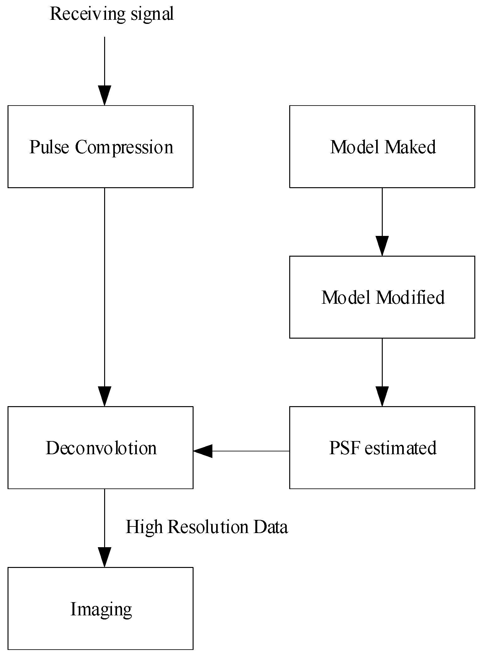
2.2. High-Resolution Pulse Compression Technology Based on Deconvolution

As previously mentioned, the pulse compression process can be written as

$$y(t)=x(t)\ast h(t)=x(t)\ast s(\tau -t)={\displaystyle {\int }_{-\infty }^{\infty }x(u)\ast s(}\tau -t+u)\mathrm{d}u=R_{xs}(t-\tau ),$$

(8)

where R_xs(t−τ) is the correlation function.

When the signal and noise are not correlated, and assuming that the echo of interest is a simple delay model, the output of the matching filter can be written as an auto-correlation function of the transmitted signal s(t).

$$y(t)=a{R}_s(t-\tau )=R_s(t)\ast a\delta (t-\tau ).$$

(9)

When M targets are present, the output of pulse compression is

$$y(t)={\displaystyle {\sum }_{k=1}^{M}a{R}_s(t-{\tau }_k)}=R_s(t)\ast {\displaystyle {\sum }_{k=1}^{M}a\delta (t-{\tau }_k)},$$

(10)

where τ_k is the echo delay of the kth target.

Let the objective function be

$$Q(t)={\displaystyle {\sum }_{k=1}^{M}a\delta (t-{\tau }_k)},$$

(11)

Thus, the received signal of the imaging sonar can be rewritten as

$$y(t)=R_s(t)\ast Q(t),$$

(12)

where Q(t) is an ideal pulse-compressed output with the characteristics of a unitary impulse response function. It can reflect the acoustic reflection structure of the target well. For the imaging sonar, Q(t) can reflect the shape of the target well. So, the method aims to solve Q(t).

2.3. Calculation of Deconvolution

A deconvolution method is introduced to solve Q(t). The Richardson–Lucy (R–L) algorithm [39,40,41], which is an optimal iterative algorithm based on Bayesian theory, is applied to solve the deconvolution problem. It is widely used in image restoration and has stable performance under low SNRs.

Firstly, denote L(∙) as the convergence distance between the true value and the estimated

$$L(p(x),q(x))={\displaystyle {\int }_{-\infty }^{\infty }p(x)\log \frac{p(x)}{q(x)}}dx,$$

(13)

where p(x),q(x) is a non-negative probability density function, L(i) is a monotonically decreasing and non-negative function, and L(p(x),q(x)) = 0 if and only if p(x) = q(x).

Then, we can obtain the following solution formula:

$$\underset{n\to \infty }{\lim }{Q}^n(t)=\arg \min L(y(t),R_s(t)\ast Q(t)),$$

(14)

$$Q^{n+1}(t)=Q^n(t)[R_s(t)·\frac{y(t)}{R_s(t)·Q^K(t)}],$$

(15)

where n represents the number of iterations.

As the iteration number increases, Qⁿ(t) can converge to a unique solution by minimizing the Csiszar discrimination.

Figure 2 represents the workflow of the proposed method. Firstly, the pulse compression is adapted for the receiving signal. Secondly, we need to estimate the Point Spread Function (PSF), which is necessary for the R–L algorithm. To estimate the PSF, the model is made to follow the transmit signal, and then modified by the response of the system. Thirdly, the calculation of deconvolution is performed by the R–L algorithm. Finally, the high-resolution data and image from the side-scan sonar are acquired.

3. Results

3.1. Numerical Simulation

The performance under different SNRs was calculated by simulation. The simulation conditions of this section were set as follows: the transmitted signal was a LFM signal, the center frequency and signal bandwidth were 500 and 50 kHz, respectively, and the pulse width length of the signal was 3.2 ms.

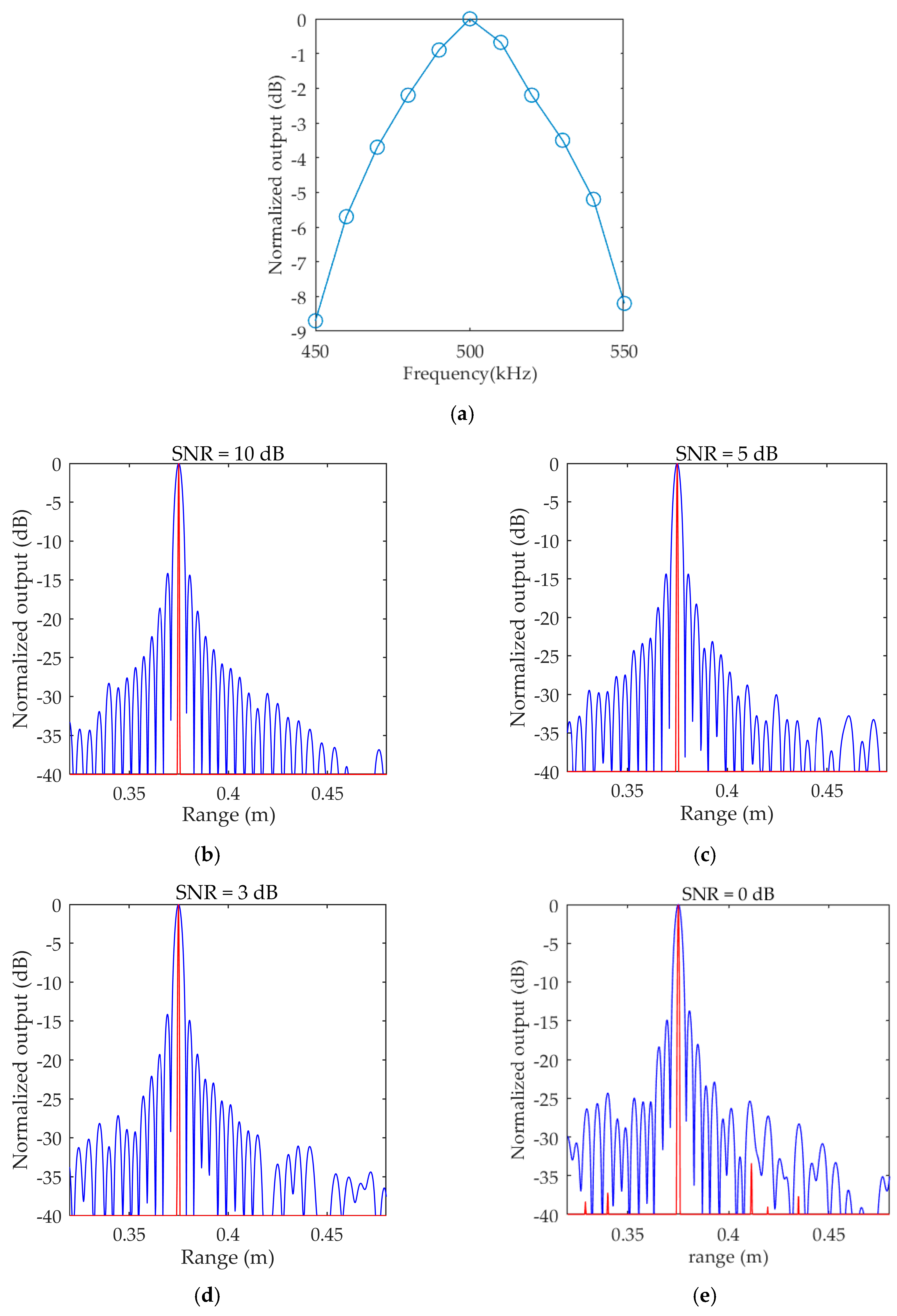
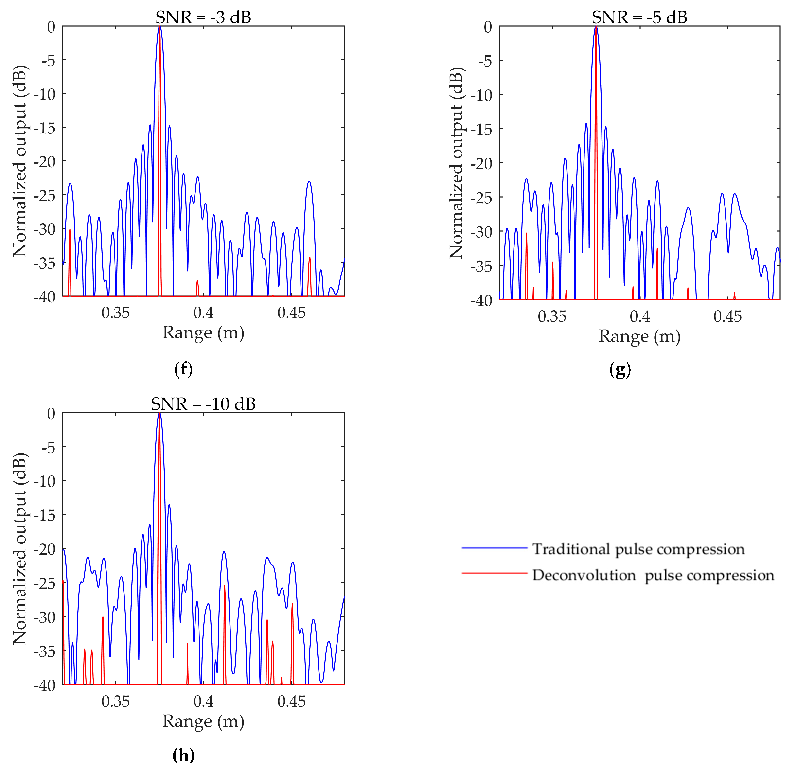
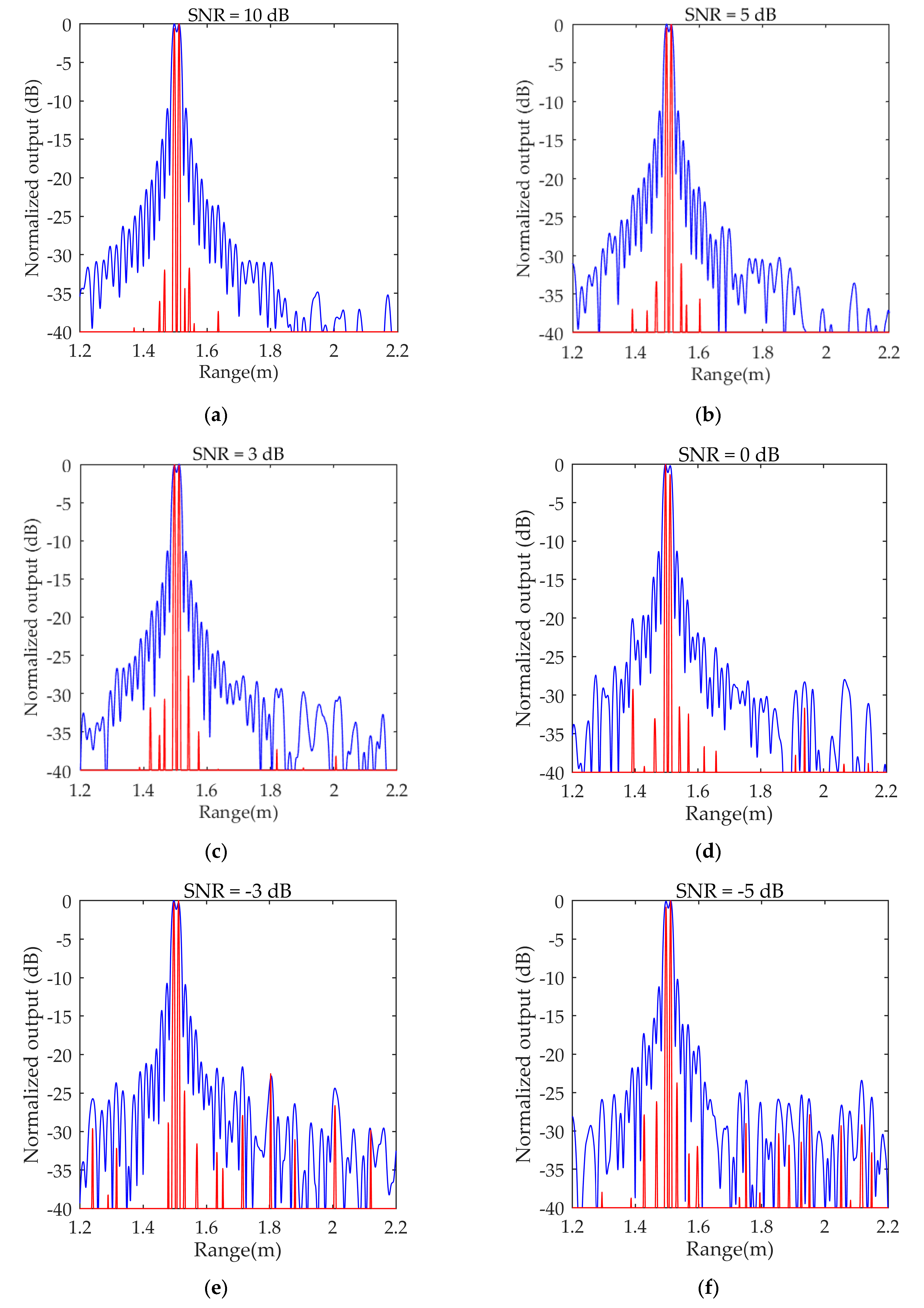
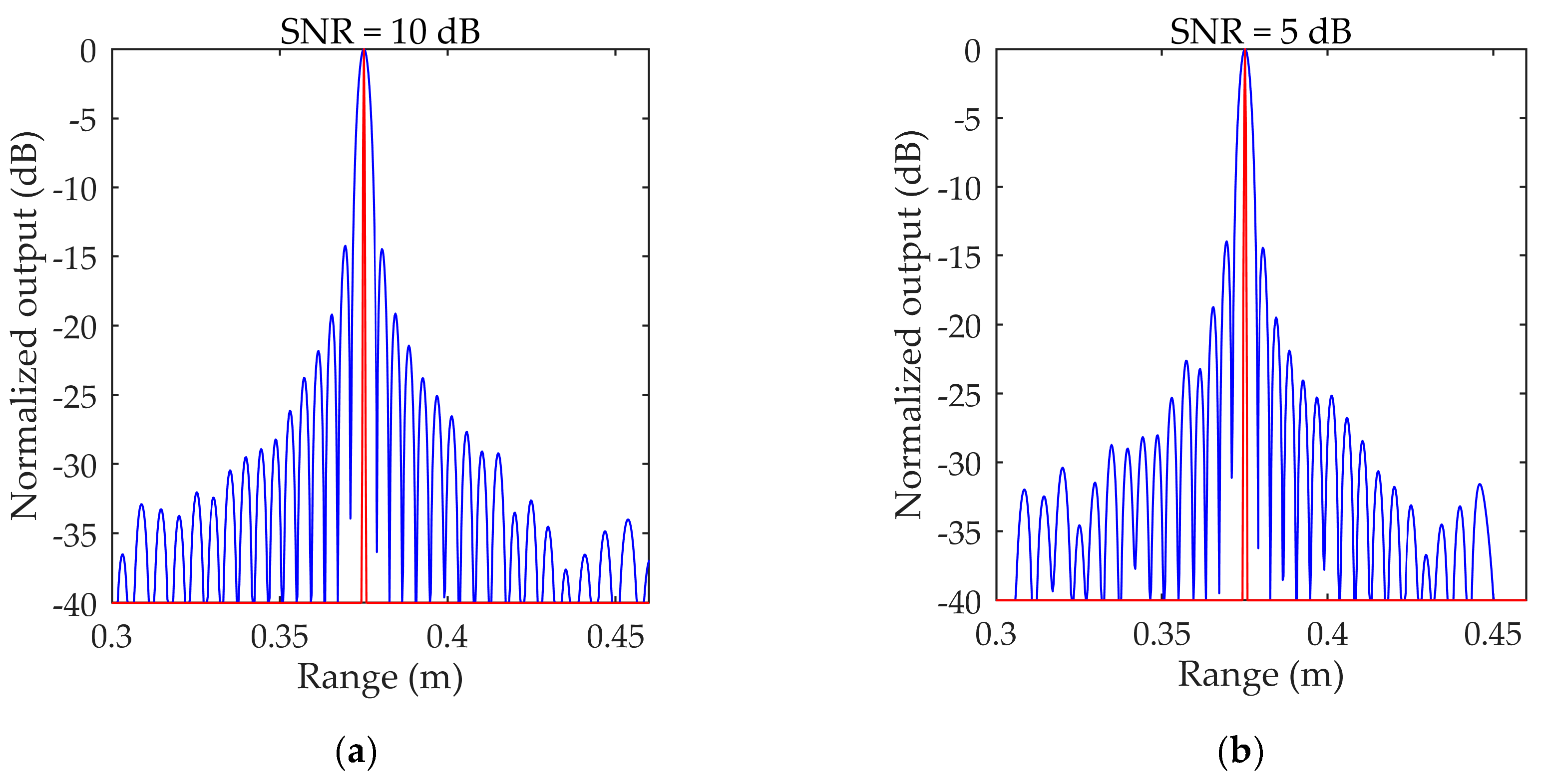
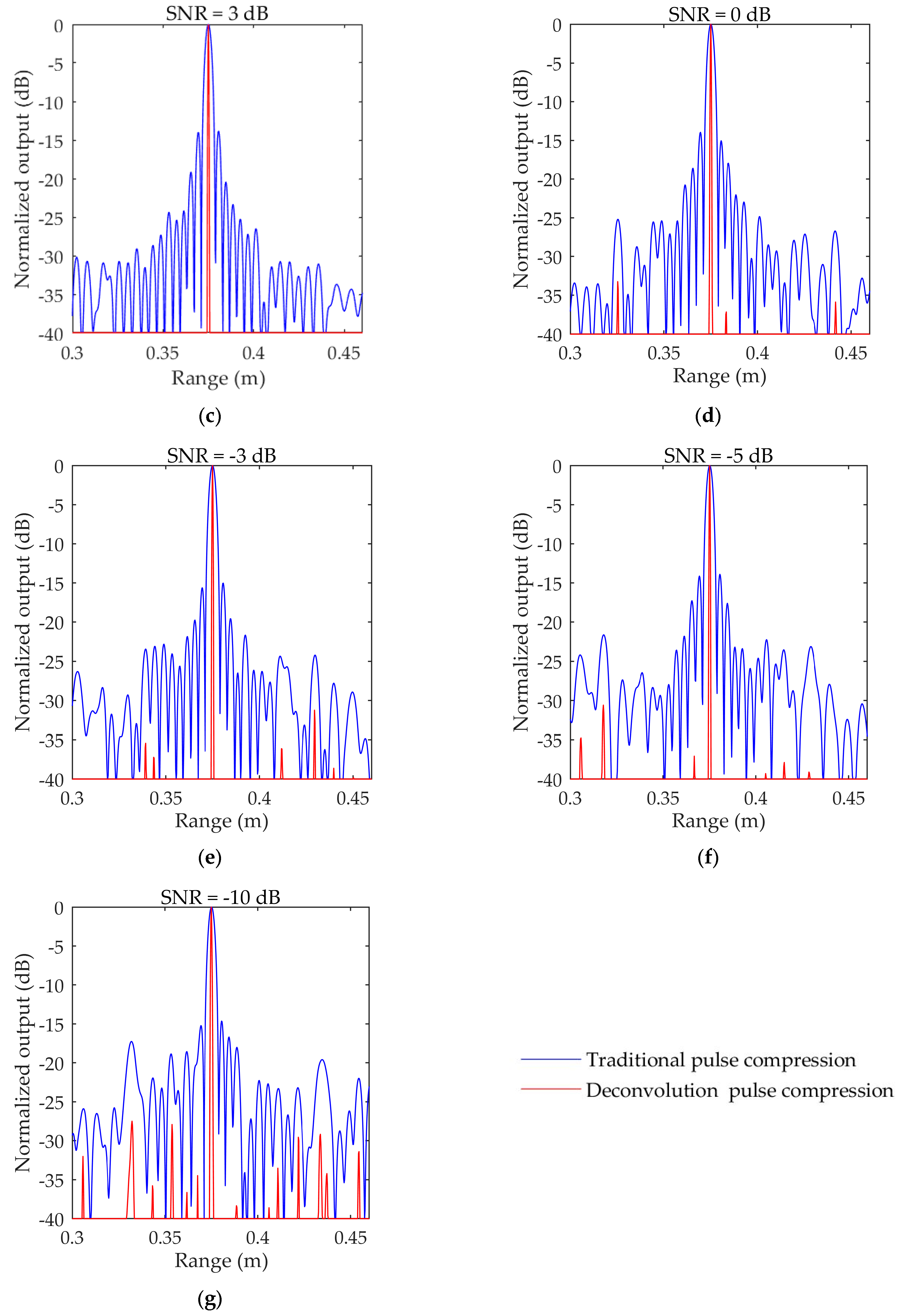
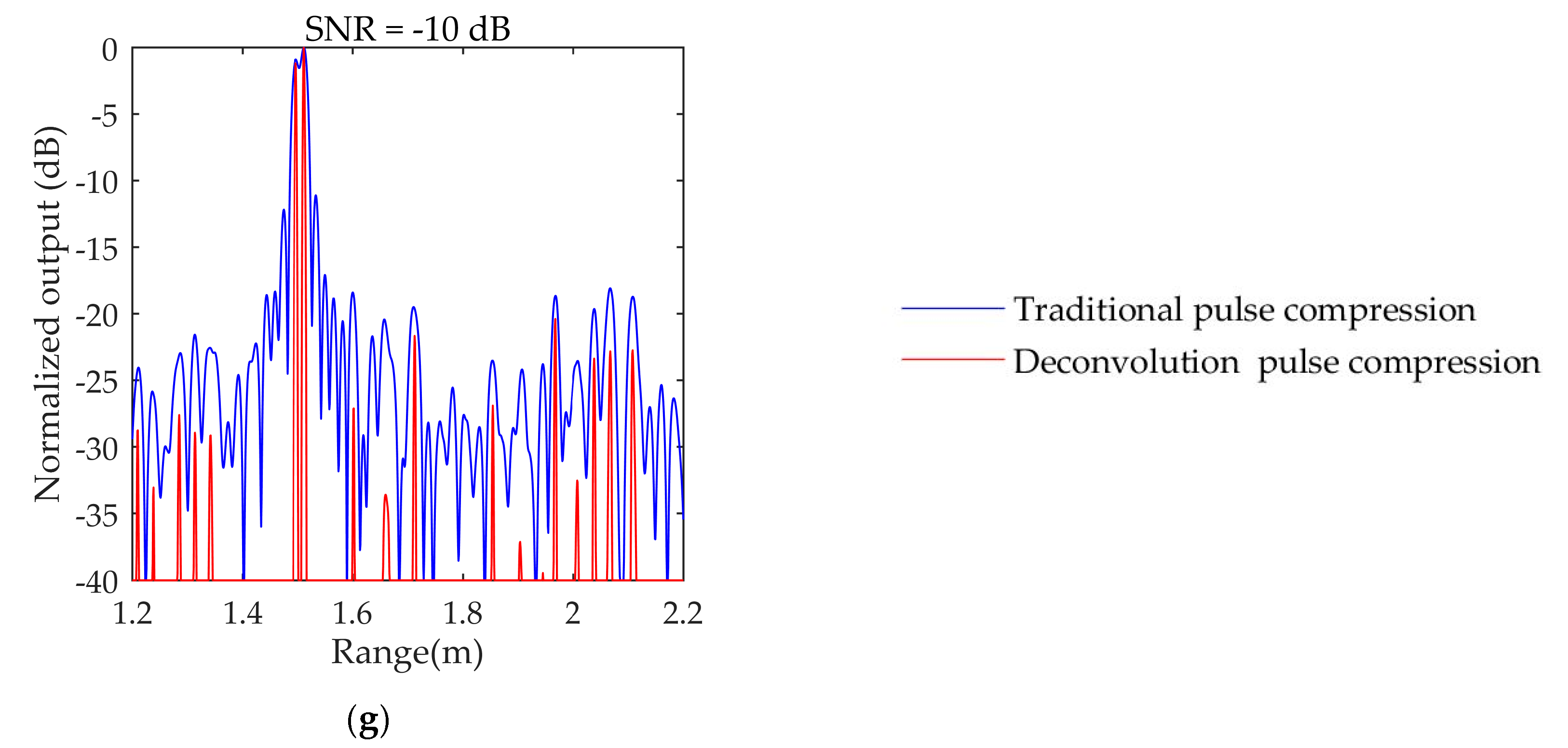
3.1.1. The Influence of Different SNRs

Firstly, we discuss the performance of pulse compressions with the deconvolution technique under different noise conditions, and the results of the traditional pulse compression technique are compared with the proposed method, as shown in Figure 3. The statistical results of the main flap width and main side ratio for both methods at different signal-to-noise ratios are shown in

Table 1. Comparison of the main lobe width and MSLR between the two methods.

SNR	Method	Main Lobe Width	MSLR
10 dB	Traditional pulse pressure	3 mm	−14 dB
	Deconvolutional pulse pressure	0.4 mm	−40 dB
5 dB	Traditional pulse pressure	3 mm	−14 dB
	Deconvolutional pulse pressure	0.4 mm	−40 dB
3 dB	Traditional pulse pressure	3 mm	−14 dB
	Deconvolutional pulse pressure	0.4 mm	−40 dB
0 dB	Traditional pulse pressure	3 mm	−14 dB
	Deconvolutional pulse pressure	0.4 mm	−36 dB
−3 dB	Traditional pulse pressure	3 mm	−14 dB
	Deconvolutional pulse pressure	0.5 mm	−30 dB
−5 dB	Traditional pulse pressure	3 mm	−14 dB
	Deconvolutional pulse pressure	0.5 mm	−28 dB
−10 dB	Traditional pulse pressure	3 mm	−14 dB
	Deconvolutional pulse pressure	0.5 mm	−24 dB

.

Compared with the processing results in Figure 3 and Table 1, the main lobe width of the deconvolution method is similar to the impact function, and it shows better range resolution and can truly reflect the objective function. The MSLR of the deconvolution method is lower and can reach more than 40 dB, which can effectively reduce the interference of strong targets on the SSS sonogram. Moreover, the algorithm has a good tolerance-to-noise ratio and maintains good performance at a SNR of −10 dB.

3.1.2. Considering the Influence of Sonar Parameters

In the actual sonar system, the signal transmission and reception process includes transmission drive, transmission electroacoustic conversion, receiving electroacoustic conversion, receiving circuit reception, etc., as shown in Figure 4.

Among these, the frequency band response of the transducer is generally not very flat. The transmission drive also leads to a distortion in the transmitted signal due to the influence of charge and discharge, and the comprehensive sonar system response leads to a mismatch in the conventional pulse compression signal model, increasing the main lobe width of pulse compression and decreasing the MSLR. This decrease in the MSLR has an adverse impact on image quality. To calculate and analyze the effect of the algorithm on practical engineering applications through simulations, the band response of the sonar system to the signal was comprehensively considered in the simulation experiment, and the simulation values are shown in Figure 5. The output results of the deconvolution method and comparison method under these conditions are also shown in Figure 5.

Through comparative analysis, we see that under the simulation conditions, due to the frequency band response caused by the sonar system, the sidelobe of conventional pulse compression technology is irregular, and the performance is significantly reduced compared with the ideal pulse compression results; however, the deconvolution technology overcomes the influence of model mismatch due to its multiple iterations of optimization and maintains a good main lobe width and MSLR.

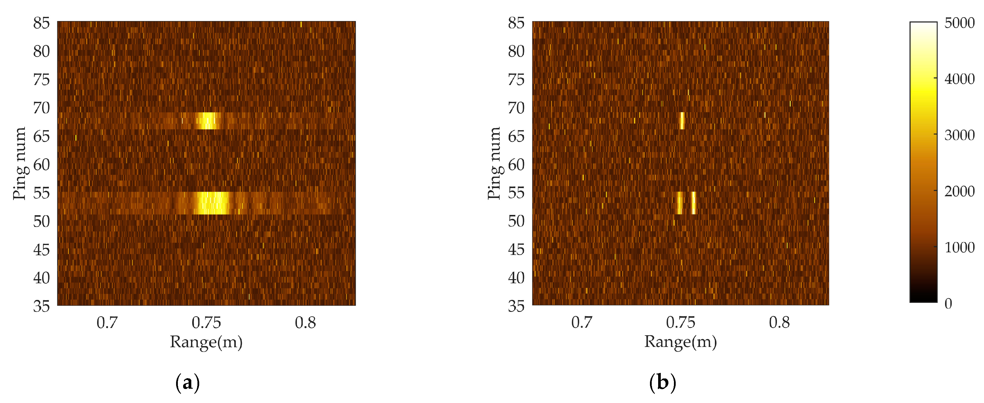
3.1.3. The Impact on Strong Interference

In practice, strong interference may lead to poor target resolution. To analyze the impact of strong interference, a simulation was performed. In the simulation, there was a target and an interference with the same intensity. The results are depicted in Figure 6.

Due to the good range resolution ability of the deconvolutional pulse compression algorithm, the distinction between the targets and interference was clearer than that of conventional pulse compression technology, and this method worked well under different SNRs.

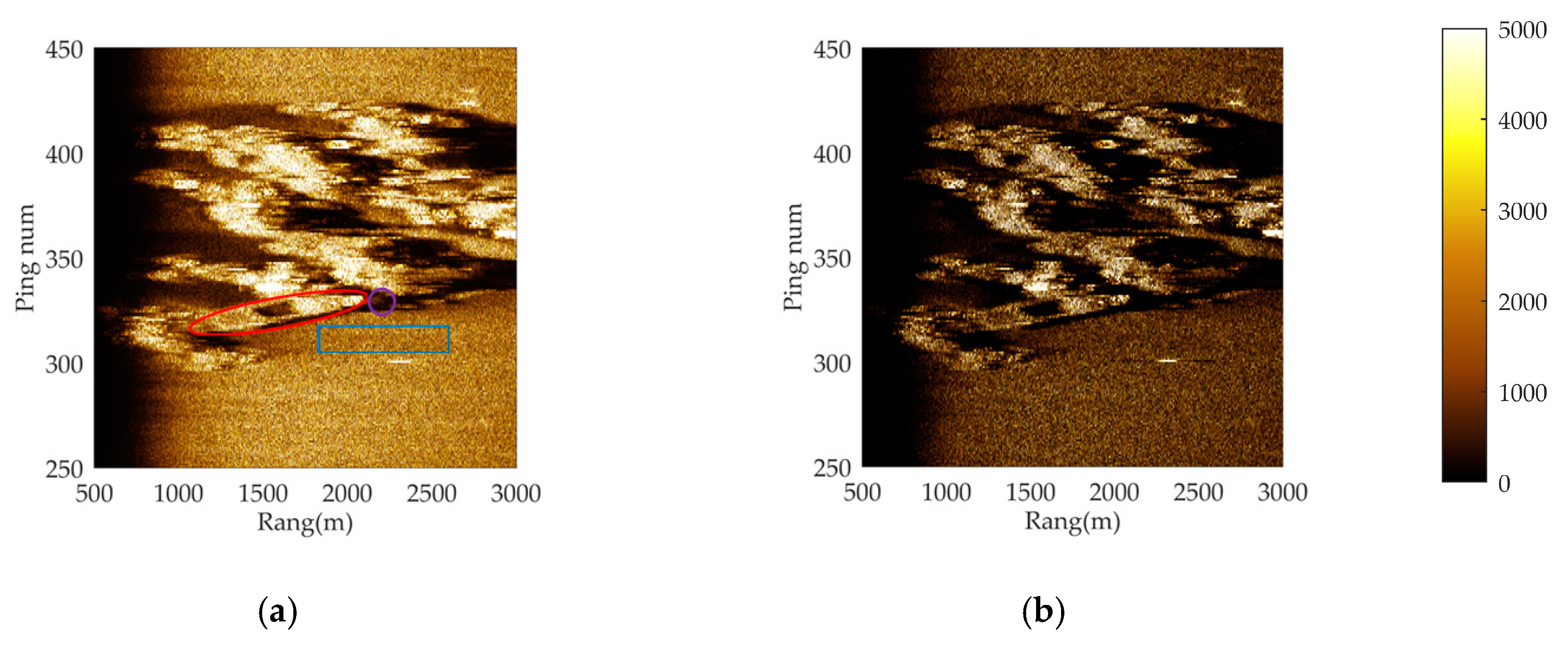
3.1.4. The Impact on Imaging

To analyze the effect of the proposed algorithm on actual imaging results, side-scan sonar imaging results were simulated, and a comparison graph of the imaging results of the two methods is shown in Figure 7. Three targets are included in the simulation graph, two of which are on the same time slice (Ping).

In comparison to Figure 7a, Figure 7b has a clearer target contour because of the improved high-resolution algorithm, and the targets at different distances at the same time can be clearly resolved. Figure 7a, with its conventional processing method, cannot realize multi-target resolution due to the lower distance resolution and stronger sidelobe interference.

3.2. Sea Experiment

For the image of SSS, there are two main types of applications. One is the large-scale imaging of the seabed, which completes the exploration of seabed topography, including the imaging detection of shipwrecks, seamounts, and trenches; the second is to search and explore small underwater targets, such as pipelines and mines. To demonstrate the performance of the algorithm, seabed and small target imaging were performed separately.

These data were obtained through the sea trials. The water depth in the trial was below 20 m.

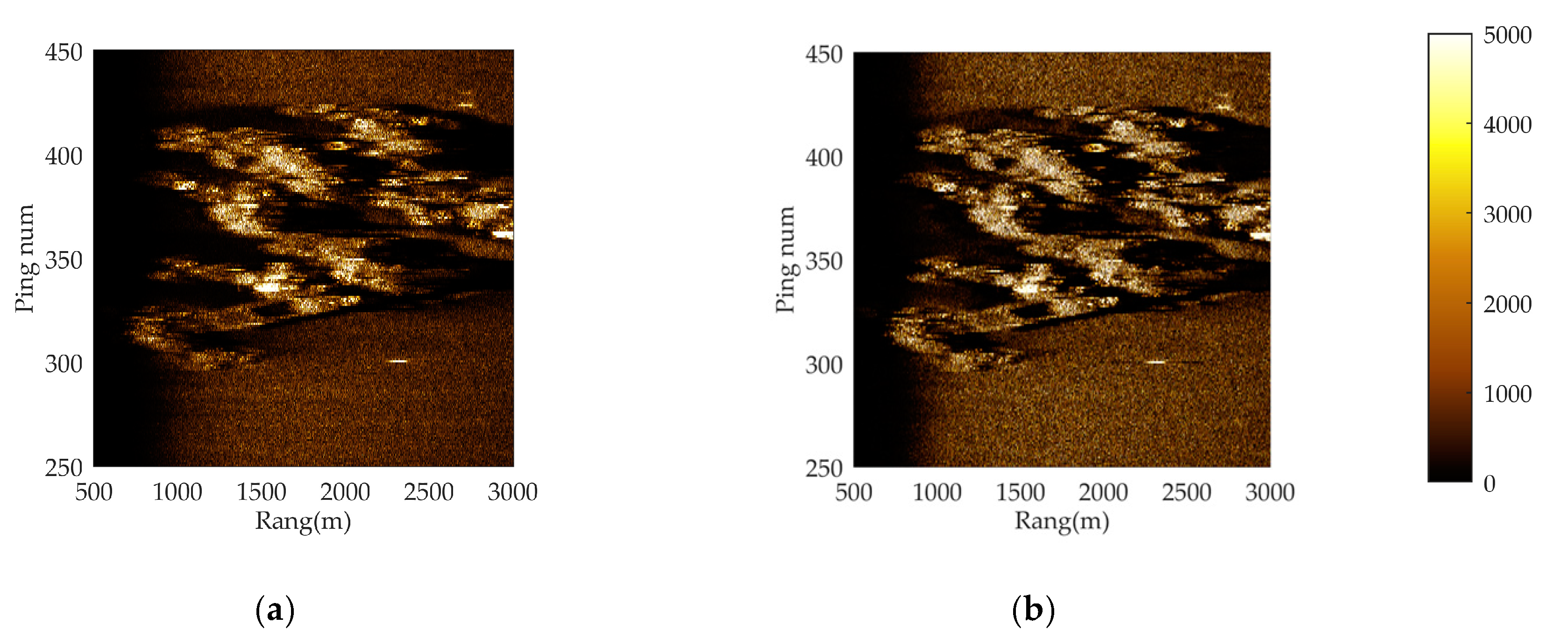
3.2.1. The Influence of the Algorithm on Seabed Imaging

Evaluation Indicators

The imaging quality of our method was analyzed in the following via the imaging effect of seabed wrecks. There are several commonly used image metrics to evaluate the clarity and prominence of objects in the image background in the field of image processing, including the SNR, contrast ratio (CR) [42], and contrast–shadow ratio (CSR) [43]. CSR is a method used to evaluate the contrast between the target and shadow. The evaluation results given are similar to those of visual evaluations, and are often used for quantitative evaluation of image quality control, performance comparison, and defect detection. The higher the value of CSR, the better the image quality. Moreover, the sharpness of the image is improved with an increase in CR. This results in a clearer outline of the target in the image and more details displayed.

The specific calculation is as follows:

$$SNR=(I_M-\overline{I_B})/\overline{I_B},$$

(16)

$$CR=(\overline{I_H}-\overline{I_B})/\overline{I_B},$$

(17)

$$CSR=(\overline{I_H}-\overline{I_S})/\overline{I_S},$$

(18)

where $I_M$ is the maximum intensity value of the highlighted areas; $\overline{I_H}$ $\overline{I_B}$, and $\overline{I_S}$ are the average intensity of the highlighted areas, seabed background areas, and seabed shadow areas, respectively.

To analyze the ability of the algorithm to maintain image sharpness, the algorithm’s mean square error (MSE), peak signal-to-noise ratio (PSNR), and structural similarity (SSIM) performance were analyzed.

For two m × n images I and K, the mean square error (MSE) was defined as

$$MSE=\frac{1}{mn}{{\displaystyle \sum _{i=0}^{m-1}{\displaystyle \sum _{j=0}^{n-1}\left[I(i,j)-K(i,j)\right]}}}^2,$$

(19)

To locate the peak signal-to-noise ratio (PSNR), we used

$$PSNR=10·{\log }_{10}(\frac{MA{X}_I^2}{MSE})=20·{\log }_{10}(\frac{MA{X}_I}{\sqrt{MSE}}),$$

(20)

where MAX_I is the maximum value that represents the color of the image; if each sample point is represented by 8 bits, then this value is 255. Thus, the smaller the MSE, the larger the PSNR; the larger the PSNR, the better the quality of the image is represented.

The structural similarity (SSIM) was calculated by

$$SSIM(x,y)={\left[l(x,y)\right]}^{\alpha }{\left[c(x,y)\right]}^{\beta }{\left[s(x,y)\right]}^{\gamma },$$

(21)

where α > 0, β > 0, and γ > 0.

$$l(x,y)=\frac{2{\mu }_x{\mu }_y+c1}{{\mu }_x^2+{\mu }_y^2+c1},$$

(22)

$$c(x,y)=\frac{2{\sigma }_{xy}+c2}{{\sigma }_x^2+{\sigma }_y^2+c2},$$

(23)

$$s(x,y)=\frac{{\sigma }_{xy}+c3}{{\sigma }_x{\sigma }_y+c3}$$

(24)

where I(x,y) is the luminance comparison, c(x,y) is the contrast comparison, and s(x,y) is the structure comparison. μ_x and μ_y represent the mean of x and y, respectively, and σ_x and σ_y represent the standard deviation of x and y, respectively. σ_xy represents the covariance between x and y. The denominator is constant to avoid the systematic error caused by zero. c1, c2, and c3 are constants to avoid the systematic error caused by the denominator being zero.

Comparative Analysis of Imaging Quality

As shown in Figure 8, the SSS image processed by pulse compression technology had a fuzzy boundary between the target and seabed background, and the target was almost integrated with the background. However, in the SSS image processed by the algorithm proposed in this paper, the sidelobe had less interference in the image, due to a reduction in sidelobe intensity; the range resolution in the lateral direction of the image was improved so that the boundary between the contour edge of the target and seabed background was more obvious; and the shape of the target in SSS image was closer to that of the actual target.

The area in the red oval in Figure 8 was taken as the area inside the target, the area in the blue box was taken as the seabed area around the target, and the area in the purple circle beside the red box was taken as the shadow of the target. The three indicators of the image obtained by the two methods were calculated, and the results are shown in

Table 2. Performance metrics of the images of SNR, CR and CSR.

Method	SNR	CR	CSR
Conventional Pulse Compression	18.7	1.6	4.8
Proposed Method	24.7	1.88	25.8
Ratio of Improvement	32%	12.5%	437%

.

Table 2 shows that the SNR, CR, and CSR of the proposed algorithm were 24.7, 1.88, and 25.8, respectively, which were improved compared with the results of the conventional pulse compression method. The ratios of improvement for SNR, CR, and CSR were 32, 12.5, and 437%, respectively.

The proposed method was compared with the conventional image mean square sharpening method, and a comparison graph is shown in Figure 9, where Figure 9a shows the results of conventional image sharpening and Figure 9b shows the results of the proposed method.

The calculated values were analyzed and are shown in

Table 3. Performance metrics of the images of MSE, PSNR and SSIM.

Method	MSE	PSNR	SSIM
Common Sharpening Method	3.34	12.83	0.59
Proposed Method	1.52	16.30	0.79

.

This comparison shows that the improved method proposed in this paper has a larger PSNR and SSIM and smaller MSE for the image compared with the conventional method, indicating that our proposed method is superior. This is because the deconvolution method improves the resolution in the original echo domain during processing. Therefore, it achieves a better signal-to-noise ratio and improved structural features than the original image and introduces smaller errors.

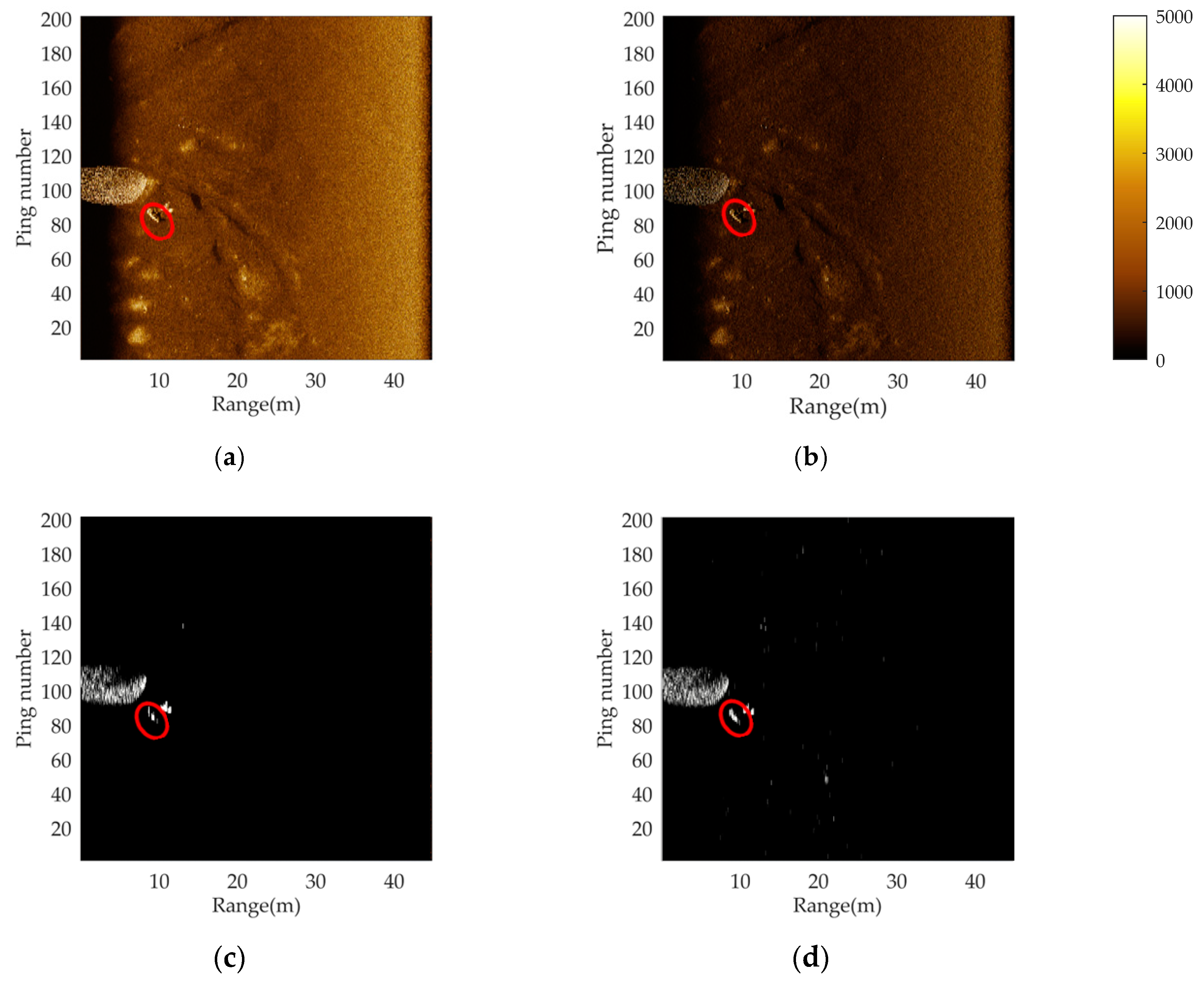
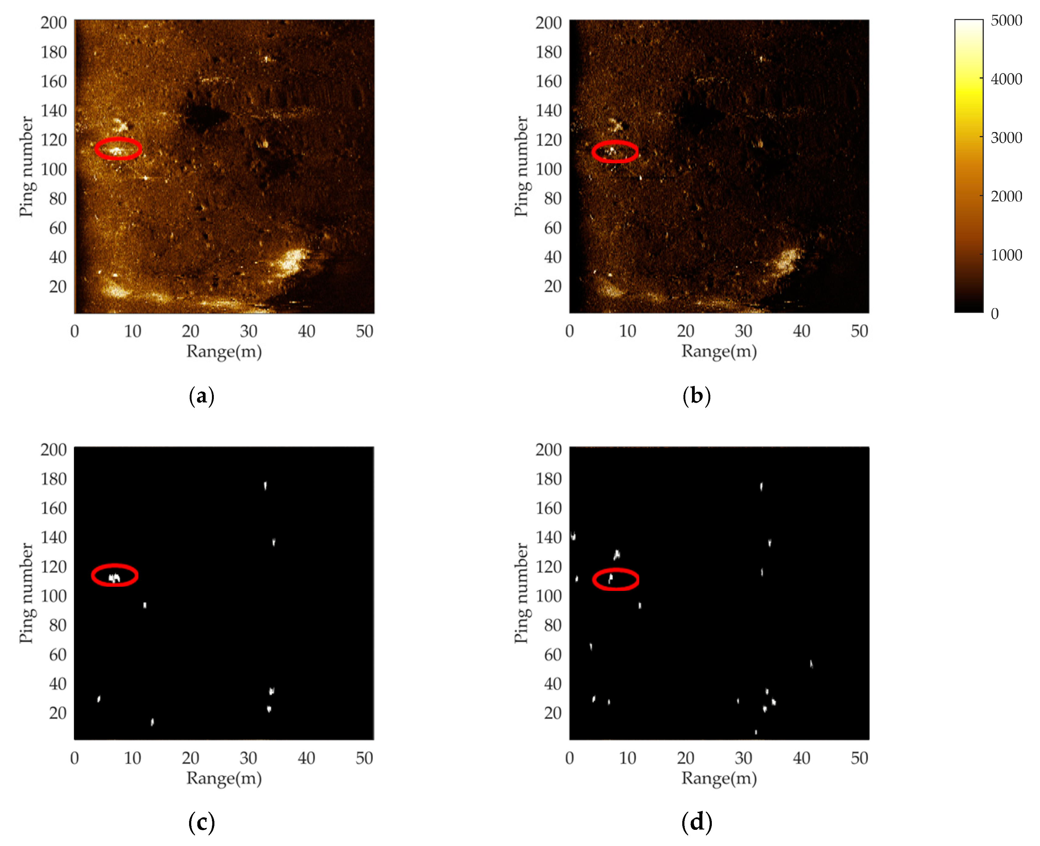
3.2.2. The Influence of the Algorithm on Target Imaging

In recent years, with the continuous progress of unmanned technology, autonomous detection technology based on SSS has developed higher requirements. Detection technology usually includes segmentation, detection, identification, and other steps. The image quality of SSS is the foundation of autonomous detection and identification algorithms.

In this section, real small targets on the seabed were imaged using the deconvolutional pulse compression method and traditional pulse compression method. The difference in image quality was assessed by independent segmentation of each acoustic image. The segmentation algorithm adopted the region growth method [44,45,46], which is characterized by ensuring the continuity of the target.

Figure 10 and Figure 11 are the processing results of the two sets of data (Data I and Data II), including the processing acoustic image of conventional pulse compression technology, the processing acoustic image of deconvolutional pulse compression algorithm, and the corresponding autonomous segmentation results. Figure 10 shows the results of Data I with a single target and image segmentation, and Figure 11 shows the imaging and segmenting results of Data II with a small target with strong interference nearby.

By comparing the processing results shown in Figure 10, we see that deconvolutional pulse compression has better resolution, and the shape of the target can be clearly described using this method. The shape of the target after autonomous segmentation is more accurate and closer to the real target, which is beneficial to the extraction of accurate target information. The follow-up detection process can effectively avoid missing judgment and misjudgment in the process of autonomous detection and processing.

Through the comparison in Figure 11, we see that in the original pulse compression processing results, due to the influence of strong interference, the target shape is difficult to clearly identify and the outline of the target is not obvious. The jamming target next to it is more similar to the target to be detected in the SSS image than the real target. Furthermore, the scale of the target after autonomous segmentation was severely distorted and was unable to maintain the target’s true form, which interferes with subsequent detection. Contrary to the results of pulse compression processing, the image obtained by deconvolutional pulse compression had smaller sidelobe interference of the target and was more clearly visible. Meanwhile, the contour was more distinct than what was obtained by conventional pulse compression processing, which is a better representation of the original shape of the target and is more conducive to subsequent segmenting. Compared with the segmentation results of pulse-compressed images, images using our proposed method were closer to the real target after segmentation.

4. Conclusions

The performance of the range resolution in high-frequency image sonar systems greatly affects image quality. As one of the important indicators for evaluating image quality, range resolution is limited by sonar system parameters. The pulse compression technology commonly used in conventional sonar signal processing is limited by the system bandwidth in terms of range resolution, and the main-to-side lobe ratio is generally high. When there is strong interference or a large quantity of debris on the seabed, it can affect the quality of the observation image. In this paper, a pulse compression technique based on deconvolution was proposed to achieve ideal objective functions. This method could be used to overcome the limitations of inherent sonar system parameters and improve range resolution without affecting system complexity.

In our simulation results, the proposed algorithm improved the main lobe width of pulse compression, and the main-to-side lobe ratio also significantly increased. In the processing results of data from actual sea trials, the proposed method effectively improved image quality. In the results of the data processing, the ratios of improvement for SNR, CR, and CSR were 32, 12.5, and 437%, respectively. Combined with object segmentation methods, the object segmentation accuracy was effectively improved, and the segmented target largely retained the morphological information of the actual target. This shows that our proposed method has great potential in autonomous detection. In addition, some high-precision ocean surveys, exploration, and seabed sedimentological surveys may also be potential applications of this method.

References

1. Nguyen, V.D.; Luu, N.M.; Nguyen, Q.K.; Nguyen, T.-D. Estimation of the Acoustic Transducer Beam Aperture by Using the Geometric Backscattering Model for Side-Scan Sonar Systems. Sensors 2023, 23, 2190. [Google Scholar] [CrossRef]
2. Meng, X.; Xu, W.; Shen, B.; Guo, X. A High–Efficiency Side–Scan Sonar Simulator for High–Speed Seabed Mapping. Sensors 2023, 23, 3083. [Google Scholar] [CrossRef]
3. Wang, Z.; Zhang, S.; Gross, L.; Zhang, C.; Wang, B. Fused Adaptive Receptive Field Mechanism and Dynamic Multiscale Dilated Convolution for Side-Scan Sonar Image Segmentation. IEEE Trans. Geosci. Remote Sens. 2022, 60, 5116817. [Google Scholar] [CrossRef]
4. Zhu, H.H.; Cui, Z.Q.; Liu, J.; Liu, X.; Wang, J.H. A Method for Inverting Shallow Sea Acoustic Parameters Based on the Backward Feedback Neural Network Model. J. Mar. Sci. Eng. 2023, 11, 1340. [Google Scholar] [CrossRef]
5. Borrelli, M.; Smith, T.L.; Mague, S.T. Vessel-Based, Shallow Water Mapping with a Phase-Measuring Sidescan Sonar. Estuaries Coast. 2022, 45, 961–979. [Google Scholar] [CrossRef]
6. Zheng, G.; Zhang, H.; Li, Y.; Zhao, J. A Universal Automatic Bottom Tracking Method of Side Scan Sonar Data Based on Semantic Segmentation. Remote Sens. 2021, 13, 1945. [Google Scholar] [CrossRef]
7. Cheng, Z.; Huo, G.; Li, H. A Multi-Domain Collaborative Transfer Learning Method with Multi-Scale Repeated Attention Mechanism for Underwater Side-Scan Sonar Image Classification. Remote Sens. 2022, 14, 355. [Google Scholar] [CrossRef]
8. Shang, X.; Zhao, J.; Zhang, H. Automatic Overlapping Area Determination and Segmentation for Multiple Side Scan Sonar Images Mosaic. IEEE J. Sel. Top. Appl. Earth Obs. Remote Sens. 2021, 14, 2886–2900. [Google Scholar] [CrossRef]
9. Brown, D.C.; Gerg, I.D.; Blanford, T.E. Interpolation Kernels for Synthetic Aperture Sonar Along-Track Motion Estimation. IEEE J. Ocean. Eng. 2020, 45, 1497–1505. [Google Scholar] [CrossRef]
10. Tuladhar, S.R.; Buck, J.R. Unit Circle Rectification of the Minimum Variance Distortionless Response Beamformer. IEEE J. Ocean. Eng. 2020, 45, 500–510. [Google Scholar] [CrossRef]
11. Wang, Q.L.; Zhu, H.H.; Chai, Z.G.; Cui, Z.Q.; Wang, Y.F. Analysis of VLF Wave Field Components and Characteristics Based on Finite Element Time-Domain Method. J. Sensors. 2023, 2023, 7702342. [Google Scholar] [CrossRef]
12. Elbir, A.M. DeepMUSIC: Multiple Signal Classification via Deep Learning. IEEE Sens. Lett. 2020, 4, 7001004. [Google Scholar] [CrossRef]
13. Yang, X.B.; Wang, K.; Zhou, P.Y.; Xu, L.; Liu, J.L.; Sun, P.P.; Su, Z.Q. Ameliorated-multiple signal classification (Am-MUSIC) for damage imaging using a sparse sensor network. Mech. Syst. Signal Process. 2022, 163, 108154. [Google Scholar] [CrossRef]
14. Yin, J.W.; Guo, K.; Han, X.; Yu, G. Fractional Fourier transform based underwater multi-targets direction-of-arrival estimation using wideband linear chirps. Appl. Acoust. 2020, 169, 107477. [Google Scholar] [CrossRef]
15. Thanh Le, H.; Phung, S.L.; Chapple, P.B.; Bouzerdoum, A.; Ritz, C.H.; Tran, L.C. Deep Gabor Neural Network for Automatic Detection of Mine-Like Objects in Sonar Imagery. IEEE Access. 2020, 8, 94126–94139. [Google Scholar] [CrossRef]
16. Zhu, H.H.; Xue, Y.Y.; Ren, Q.Y.; Liu, X. Inversion of shallow seabed structure and geoacoustic parameters with waveguide characteristic impedance based on Bayesian approach. Front. Mar. Sci. 2023, 10, 1104570. [Google Scholar] [CrossRef]
17. Yu, Y.C.; Zhao, J.H.; Gong, Q.H.; Huang, C.; Zheng, G.; Ma, J. Real-time underwater maritime object detection in side-scan sonar images based on transformer-YOLOv5. Remote Sens. 2021, 13, 3555. [Google Scholar] [CrossRef]
18. Połap, D.; Wawrzyniak, N.; Włodarczyk-Sielicka, M. Side-scan sonar analysis using roi analysis and deep neural networks. IEEE Trans. Geosci. Remote Sens. 2022, 60, 4206108. [Google Scholar] [CrossRef]
19. Sun, Y.; Liu, Q.; Cai, J.; Long, T. A Novel Weighted Mismatched Filter for Reducing. IEEE Trans. Aerosp. Electron. Syst. 2019, 55, 1450–1460. [Google Scholar] [CrossRef]
20. Xia, D.; Zhang, L.; Wu, T.; Hu, W. An interference suppression algorithm for cognitive bistatic airborne radars. J. Syst. Eng. Electron. 2022, 33, 585–593. [Google Scholar] [CrossRef]
21. Lønmo, T.I.B.; Austeng, A.; Hansen, R.E. Improving swath sonar water column imagery and bathymetry with adaptive beamforming. IEEE J. Ocean. Eng. 2020, 45, 1552–1563. [Google Scholar] [CrossRef]
22. Guan, C.Y.; Zhou, Z.M.; Zeng, X.W. A phase-coded sequence design method for active sonar. Sensors 2020, 20, 4659. [Google Scholar] [CrossRef] [PubMed]
23. Zhang, X.; Ying, W.; Dai, X. High-resolution imaging for the multireceiver SAS. J. Eng. Technol. 2019, 19, 6057–6062. [Google Scholar] [CrossRef]
24. Zeng, X.; Liu, J.; Gao, B. Three-dimensional Imaging Sonar Signal Processing System Based on Blade Server. J. Phys. Conf. Ser. 2019, 1213, 042061. [Google Scholar] [CrossRef]
25. Sun, D.; Ma, C.; Mei, J.; Shi, W. Improving the resolution of underwater acoustic image measurement by deconvolution. Appl. Acoust. 2020, 165, 107292. [Google Scholar] [CrossRef]
26. Bai, C.; Liu, C.; Jia, H. Compressed blind deconvolution and denoising for complementary beam subtraction light-sheet fluorescence microscopy. IEEE. Trans. Biomed. Eng. 2019, 66, 2979–2989. [Google Scholar] [CrossRef]
27. Xue, Y.Y.; Zhu, H.H.; Wang, X.H. Bayesian geoacoustic parameters inversion for multi-layer seabed in shallow sea using underwater acoustic field. Front. Mar. Sci. 2023, 10, 1058542. [Google Scholar] [CrossRef]
28. Wang, P.; Chi, C.; Ji, Y.Q.; Huang, Y.; Huang, H.N. Two-dimensional deconvoled beamforming for the high-resolution underwater three-dimensional acoustical imaging. Acta Acust. 2019, 44, 613–625. [Google Scholar]
29. Zhu, J.H.; Song, Y.P.; Jiang, N.; Xie, Z.; Fan, C.Y.; Huang, X.T. Enhanced Doppler Resolution and Sidelobe Suppression Per-formance for Golay Complementary Waveforms. Remote Sens. 2023, 15, 2452. [Google Scholar] [CrossRef]
30. Zhang, X.B.; Yang, P.X.; Sun, H.X. An omega-k algorithm for multireceiver synthetic aperture sonar. Electron. Lett. 2023, 59, e12859. [Google Scholar] [CrossRef]
31. Mei, J.D.; Shi, W.P.; Ma, C.; Sun, D.J. Near-field beamforming acoustic image measurement based on decovolution. Acta Acust. 2020, 45, 15–28. [Google Scholar]
32. Teng, T.T.; Liu, H.M.; Sun, D.S.; Xi, J.C.; Qu, G.Y.; Yang, S. Active sonar de-convolution matched filtering method. In Proceedings of the 2018 IEEE International Conference on Signal Processing, Communications and Computing (ICSPCC), Qingdao, China, 14–16 September 2018. [Google Scholar]
33. Shang, Z.G.; Qu, X.H.; Qiao, G.; Hao, C.P. Localizing mixed far- and near-field sources using beamforming deconvolution techniques. Acta Acust. 2023, 48, 447–458. [Google Scholar]
34. Guo, W.; Piao, S.C.; Yang, T.C.; Guo, J.Y.; Iqbal, K. High-resolution power spectral estimation method using deconvolution. IEEE J. Ocean. Eng. 2020, 45, 489–499. [Google Scholar] [CrossRef]
35. Yang, T.C. Deconvolved conventional beamforming for a horization line array. IEEE J. Ocean. Eng. 2018, 43, 160–172. [Google Scholar] [CrossRef]
36. Sun, D.J.; Ma, C.; Yang, T.C.; Mei, J.D.; Shi, W.P. Improving the performance of a vector sensor line array by deconvolution. IEEE J. Ocean. Eng. 2020, 45, 1063–1077. [Google Scholar] [CrossRef]
37. Liu, X.H.; Fan, J.H.; Sun, C.; Yang, Y.X.; Zhuo, J. High-resolution and low-sidelobe forward-look sonar imaging using deconvolution. Appl. Acoust. 2021, 178, 107986. [Google Scholar] [CrossRef]
38. Liu, X.H.; Shi, R.W.; Sun, C.; Yang, Y.X.; Zhuo, J. Using deconvolution to suppress range sidelobes for MIMO sonar imaging. Appl. Acoust. 2022, 186, 108491. [Google Scholar] [CrossRef]
39. Richardson, W.H. Bayesian-based iterative method of image restoration. J. Opt. Soc. Am. 1972, 62, 55–59. [Google Scholar] [CrossRef]
40. Lucy, L.B. An iterative technique for the rectification of observed distributions. Astron. J. 1974, 79, 745–754. [Google Scholar] [CrossRef]
41. Fish, D.A.; Brinicomde, A.M.; Pike, E.R. Blind deconvolution by means of the Richards-Lucy algorithm. J. Opt. Soc. Am. 1995, 12, 58–65. [Google Scholar] [CrossRef]
42. Yang, L.; Yang, Y.; Hasna, M.O. Coverage, probability of SNR gain, and DOR analysis of RIS-aided communication systems. IEEE Wireless Commun. Lett. 2020, 9, 1268–1272. [Google Scholar] [CrossRef]
43. Wang, X.Y.; Wang, L.Y.; Li, G.L.; Xie, X. A robust and fast method for sidescan sonar image segmentation based on region growing. Sensors 2021, 21, 6960. [Google Scholar] [CrossRef] [PubMed]
44. Li, J.; Jiang, P.; Zhu, H. A local region-based level set method with Markov random field for side-scan sonar image multi-level segmentation. IEEE Sens. J. 2020, 21, 510–519. [Google Scholar] [CrossRef]
45. Wang, H.; Gao, N.; Xiao, Y. Image feature extraction based on improved FCN for UUV side-scan sonar. Mar. Geophys. Res. 2020, 41, 18. [Google Scholar] [CrossRef]
46. Wang, Z.; Guo, J.; Huang, W. Side-scan sonar image segmentation based on multi-channel fusion convolution neural networks. IEEE Sens. J. 2022, 22, 5911–5928. [Google Scholar] [CrossRef]
Figure 1. The geometry of target detection by sonar.
Remotesensing 15 04908 g001
Figure 2. The workflow diagram of the proposed method.
Remotesensing 15 04908 g002
Figure 3. The simulation results of pulse compression and deconvolutional pulse compression under different SNRs: (a) simulation results under 10 dB; (b) simulation results under 5 dB; (c) simulation results under 3 dB; (d) simulation results under 0 dB; (e) simulation results under −3 dB; (f) simulation results under −5 dB; and (g) simulation results under −10 dB.
Remotesensing 15 04908 g003aRemotesensing 15 04908 g003b
Figure 4. The signal generation process of the SSS system.
Remotesensing 15 04908 g004
Figure 5. Comparison of deconvolution results and conventional pulse pressure under the influence of sonar parameters: (a) frequency response of the sonar; (b) simulation results under 10 dB; (c) simulation results under 5 dB; (d) simulation results under 3 dB; (e) simulation results under 0 dB; (f) simulation results under −3 dB; (g) simulation results under −5 dB; and (h) simulation results under −10 dB.
Remotesensing 15 04908 g005aRemotesensing 15 04908 g005b
Figure 6. Comparison of deconvolution results with conventional pulse compression under the influence of strong interference: (a) simulation results under 10 dB; (b) simulation results under 5 dB; (c) simulation results under 3 dB; (d) simulation results under 0 dB; (e) simulation results under −3 dB; (f) simulation results under −5 dB; and (g) simulation results under −10 dB.
Remotesensing 15 04908 g006aRemotesensing 15 04908 g006b
Figure 7. The simulated images with targets were obtained by (a) the traditional method and (b) the proposed method.
Remotesensing 15 04908 g007
Figure 8. SSS image processing results: (a) SSS images processed by conventional pulse compression, where the red oval represents the target area, the purple circle represents the shadow area, and the blue rectangle represents the botttom area, respectively; (b) SSS images processed by the proposed method.
Remotesensing 15 04908 g008
Figure 9. The SSS image processing results: (a) SSS images processed by the sharpening method and (b) SSS images processed by the proposed method.
Remotesensing 15 04908 g009
Figure 10. A comparison of processing results between the conventional pulse compression technique and proposed method: (a) imaging results of conventional pulse compression technology; (b) imaging results of the proposed method; (c) image segmentation results after imaging by conventional pulse compression technology; and (d) image segmentation results after imaging by the proposed method. The red ovals represent the small target area.
Remotesensing 15 04908 g010
Figure 11. A comparison of processing results under strong interference conditions between the conventional pulse compression technique and proposed method: (a) imaging results of conventional pulse compression technology; (b) imaging results of the proposed method; (c) image segmentation results after imaging by conventional pulse compression technology; and (d) image segmentation results after imaging by the proposed method. The red ovals represent the small target area.
Remotesensing 15 04908 g011