Adaptive Beamforming with Sidelobe Level Control for Multiband Sparse Linear Array

Abstract

Multiband antenna arrays have the capability of effectively working in multiple frequency bands and thus significantly simplify the antenna system. To further reduce the system overhead, this paper discusses the joint design of antenna selection and adaptive beamforming for multiband antenna arrays, where the sidelobe level is also controlled so as to alleviate the effect of unknown sporadic interference. Based on the maximum signal-to-interference-plus-noise ratio (SINR) criterion and sidelobe level constraints, the proposed multiband sparse array design is formulated into a nonconvex constrained nonlinear optimization problem with an $l_{0,2}$-mixed norm regularization. This problem ensures that the same antenna positions are selected at all operating frequencies while the beamformer weights of each frequency are optimized independently. By exploiting the semi-definite relaxation and the reweighted $l_{1,\infty }$-norm approximation, the problem is converted into a series of convex subproblems and is then effectively solved by the proposed iterative reweighted method. Numerical results show that the proposed multiband sparse array significantly reduces the sidelobe levels in all operating frequencies while maintaining the maximum SINR, so it provides superior performance of interference suppression.

1. Introduction

A multiband antenna is a specialized type of antenna that is designed to effectively operate across multiple preset frequency bands simultaneously. This versatile technology substantially reduces the volume, cost, weight, and complexity associated with antenna systems. As a result, multiband antennas are increasingly being used in advanced communication and radar systems [1,2,3]. With the increasing requirement on the spatial resolution and capacity, several kinds of multiband arrays have been developed for the application of next-generation wireless communication [4]. However, in the utilization of medium- or large-scale multiband arrays, the cost, hardware complexity, and power consumption are high. Sparse arrays offer significant advantages in terms of reducing the system complexity and hardware overhead. Compared to conventional uniform linear arrays, sparse arrays use fewer antenna elements and radio-frequency channels while they have the same array aperture and suffer from only a little performance loss. Therefore, one promising direction in developing multiband antenna arrays is to design optimal sparse array configurations. Different from conventional sparse arrays working at a single frequency, the configuration of a multiband sparse array should possess the capability to deliver excellent performance across all operating frequencies, tailored to specific functions such as transmit beampattern synthesis or adaptive receive beamforming.

The design of narrowband sparse arrays, specifically focusing on single-frequency operation, has been widely explored in various tasks and performance metrics [5,6,7,8,9,10,11,12,13,14,15,16,17,18,19,20,21,22]. Depending on the application and the performance metrics, sparse array design can be divided into two categories: environment-independent or environment-dependent. In the environment-independent case, various structured sparse arrays, including minimum redundancy arrays [5], nested arrays [6], and co-prime arrays [7], have been developed to improve the direction-of-arrival (DOA) estimation performance, and then to provide good beamforming performance [8,9]. Furthermore, to obtain a sparse array with the smallest element number, sparsity-promoting algorithms for unstructured sparse arrays are used to synthesize the desired beampattern [10] or to improve the parameter estimation performance [11]. The representative algorithms include reweighted $l_1$-norm [10,12,13], mixed norm or norm combination [14], nonconvex $l_p$-norm ($0<p<1$) [15], soft-thresholding shrinkage [16], and Bayesian inference [17]. In the environment-dependent case, joint optimization of antenna position and receive beamformer has been utilized to maximize output signal-to-interference-plus-noise ratio (SINR) by exploiting environmental data. These methods have been implemented by using reweighted $l_1$-norm and semi-definite relaxation (SDR) [18], sequential convex approximation (SCA) [19], and the alternating direction method of multipliers (ADMM) [20], to name a few. Additional constraints have also been introduced to achieve sidelobe level (SLL) control [21]. To further minimize the number of required antennas, an $l_0$-norm concave approximation approach has been proposed in [22]. Since the unstructured sparse array designs are commonly coined as nonconvex constrained optimization problems, the main challenge is how to resolve these problems efficiently. Due to the powerful capability of deep neural networks (DNNs) in solving nonlinear problems and performing fast computations, a fully connected DNN has recently been applied to select antenna positions for adaptive beamforming [23,24].

Along with the continuous development of narrowband sparse arrays, wideband sparse array design has also been studied extensively in the past two decades [25,26,27,28,29,30,31,32]. Due to the significantly degraded performance of narrowband sparse arrays when the signal bandwidth increases and the narrowband hypothesis no longer holds, which results in a poor ability of interference suppression, it is necessary to consider wideband sparse array design. By utilizing a limited number of available antennas, the wideband sparse array design offers more degrees-of-freedom (DoFs) to control the beampattern over the frequencies of interest. In wideband beamforming, there are two commonly used implementation schemes: tapped delay line (TDL) filtering and discrete Fourier transform (DFT)-based sub-band processing. Concretely, TDL implements temporal filtering by using a TDL to capture the signal at different time instants, while DFT processes the signal in several narrow sub-bands via DFT [33].

Based on the TDL and DFT schemes, several different goals involving frequency-invariant (FI) beampattern synthesis, SLL control, and robust beampattern design [25,26,27] have been achieved by many wideband sparse array design methods. To be specific, FI beampattern synthesis is dedicated to generating a specific pattern regardless of the operation frequency, the SLL control aims to reduce the power of sidelobes around the mainlobe, and the robust beampattern design focuses on maintaining desired beampatterns that are not influenced by the array uncertainties or the changes of operating environment. Early methods such as simulated annealing [28,29] and genetic algorithms [30], which rely on heuristic methods, have been abandoned due to their high computational cost. Recently, the sparsity-promoting algorithm has emerged as a prevalent solution to optimizing the array design. For TDL implementation, FI beampatterns with a small number of antennas are synthesized by several effective algorithms, including reweighted $l_1$-norm [27], second-order cone programming (SOCP) [26], and the generalized matrix pencil method [34]. Although these algorithms demonstrate outstanding performance, they are still computationally expensive and thus not suitable for large-scale arrays. In contrast, DFT-based sub-band processing has become increasingly popular due to its remarkable computational efficiency [31,32]. In this approach, the wideband signal is divided into several narrow sub-bands via DFT. The beams in each sub-band are optimized by imposing group sparsity constraints through convex optimization techniques. This method has demonstrated commendable performance while demanding lower computational requirements than TDL-based approaches. However, it requires storing blocked received signals and updating the weights block by block.

In this paper, we consider the multiband sparse array design for adaptive beamforming, which is partially distinct from existing narrowband and wideband sparse array design. Since the multiband array works simultaneously at multiple frequencies, it can be considered as a narrowband array at each frequency. That is to say, the design of a multiband sparse array is equivalent to the joint design of multiple narrowband sparse arrays with the same antenna positions. From another perspective, the multiband sparse array design can be considered as a special case of the DFT-based wideband sparse array design, in which only partial DFT bins exist. However, the number of DFT bins depends on the bandwidth of the multiband antenna. Hence, the DFT-based wideband schemes will be inefficient when the frequency spacing between adjacent operation frequency bands is large enough. For multiband sparse arrays, ref. [35] utilized the linear Cantor fractal array to construct a structured sparse multiband array and then offered a Kalman filtering-based adaptive beamformer. Ref. [31] considered the joint design of antenna selection and adaptive beamformer by using group sparse regularization. The array has the same antenna position in all frequencies, while the beamforming weights of each frequency are separately optimized. However, the SLL control of receive beampattern is not taken into account. Uncontrollable high sidelobes generated at some operating frequencies will reduce the interference suppression performance, especially when unknown sporadic interference appears.

Based on the above observations, this paper discusses the problem of multiband sparse array design for adaptive beamforming with SLL control. Concretely, we jointly design an antenna selection and adaptive beamformer under the maximum SINR criterion and the SLL constraints. Since it is essential for the antenna positions to be identical in all operating frequencies, we coin the proposed sparse array design as a nonconvex constrained nonlinear optimization problem with an $l_{0,2}$-mixed norm regularization. The proposed problem is intractable since the objective function and all constraints are nonconvex, and the beamforming weights of different frequencies are coupled in the objective function. By employing the reweighted norm transformation and SDR techniques, we construct an iterative reweighted method to solve this problem effectively. With the aid of the reweighted norm approximation technique, we first equivalently express the original problem as a series of $l_{1,\infty }$-norm regularized nonconvex constrained optimization subproblems. By using SDR and linear fractional SDR schemes, we then relax the $l_{1,\infty }$-norm regularized nonconvex subproblem to the corresponding convex subproblem, which is tractably resolved by off-the-shelf toolboxes. Numerical results demonstrate that the proposed method can effectively reduce the SLL across all operating frequencies, thereby enhancing its interference suppression performance.

The remainder of this paper is organized as follows. Section 2 introduces the signal model of adaptive beamforming for multiband arrays. Section 3 states the problem formulation of multiband sparse array design for maximizing the output SINR under SLL constraints and then provides an SDR-based iterative reweighted solution algorithm. Section 4 analyzes the computational complexity of the proposed algorithm. Numerical experiments are conducted in Section 5 to validate the superiority of the optimized multiband sparse array. Section 6 provides some discussions regarding the multiband sparse array design. Concluding remarks follow at the end.

$Notations$: Throughout this paper, lower-case bold characters and upper-case bold characters represent vectors and matrices, respectively. ${(·)}^T$ indicates the transpose and ${(·)}^H$ denotes the conjugate transpose. $|·|$ is the modulus operator. $\mathbb{E}\{·\}$ denotes the statistical expectation. $\mathrm{Tr}(·)$ and $\mathrm{Rank}(·)$ stand for the trace and the rank operations, respectively. ${\mathbf{I}}_N$ stands for an $N\times N$ identity matrix. $\mathbf{W}⪰0$ means that $\mathbf{W}$ is positive semi-definite. $\mathfrak{R}\{·\}$ and $\mathfrak{I}\{·\}$ represent the real and imaginary parts of the complex variables, respectively.

2. Signal Model

Assume that the multiband array, consisting of N uniformly spaced multiband antenna elements, has the capability of receiving narrowband signals belonging to M frequency bands centered at the frequency ${\omega }_i(i=1,\dots ,M)$, respectively. Consider a desired source operating in the i-th band with the center frequency ${\omega }_i$, while there exist $P_i$ sources of interference. Both the desired source and interference signals impinge on the N-element multiband array. The baseband signal received by the multiband array at the frequency ${\omega }_i$ is given by

$${\mathbf{x}}_{{\omega }_i}={\alpha }_i\mathbf{a}\left({\theta }_{s_i},{\omega }_i\right)+\sum _{p_i=1}^{P_i}{\beta }_{p_i}\mathbf{a}\left({\theta }_{p_i},{\omega }_i\right)+{\mathbf{v}}_i,$$

(1)

where ${\mathbf{v}}_i\in {\mathbb{C}}^N$ is the additive, while Gaussian noises with variance ${\sigma }_{v_i}^2$, ${\alpha }_i,{\beta }_{p_i}\in \mathbb{C}$ are the complex amplitudes of the incident baseband source and the $p_i$-th interference source, respectively; $\mathbf{a}\left({\theta }_{s_i},{\omega }_i\right)$ and $\mathbf{a}\left({\theta }_{p_i},{\omega }_i\right)$ are the steering vectors at the frequency ${\omega }_i$ with respect to the desired source with the direction ${\theta }_{s_i}$ and the interference source with the direction ${\theta }_{p_i}$, which are defined by

$$\mathbf{a}\left({\theta }_{s_i},{\omega }_i\right)=[1,e^{j\frac{2\pi }{{\lambda }_{{\omega }_i}}dcos{\theta }_{s_i}},\dots ,e^{j\frac{2\pi }{{\lambda }_{{\omega }_i}}d\left(N-1\right)cos{\theta }_{s_i}}{]}^T$$

(2)

where d is the element spacing and ${\lambda }_{{\omega }_i}$ is the wavelength at the frequency ${\omega }_i$. To prevent spatial aliasing, we set $d=\frac{{\lambda }_{{\omega }_m}}{2}$, where ${\omega }_m$ is the highest frequency of ${\left\{{\omega }_i\right\}}_{i=1}^M$. Then the steering vector $\mathbf{a}\left({\theta }_{s_i},{\omega }_i\right)$ can be simplified as

$$\mathbf{a}\left({\theta }_{s_i},{\omega }_i\right)=[1,e^{j\pi \frac{{\omega }_i}{{\omega }_m}cos{\theta }_{s_i}},\dots ,e^{j\pi \frac{{\omega }_i}{{\omega }_m}\left(N-1\right)cos{\theta }_{s_i}}{]}^T$$

(3)

The received signal ${\mathbf{x}}_{{\omega }_i}$ is linearly combined by a beamformer at the receiver to maximize the output SINR. Denote ${\mathbf{w}}_i={\left[w_1,\dots ,w_N\right]}^T\in {\mathbb{C}}^N$ as the beamformer weight vector. Then the output of the beamformer is

$$y_{w_i}={\mathbf{w}}_i^H{\mathbf{x}}_{w_i},i=1,\dots ,M.$$

(4)

Let the adaptive beamformers be used at all frequencies ${\left\{{\omega }_i\right\}}_{i=1}^M$. Based on the maximum SINR (maxSINR) criterion, the optimal beamformers of all frequencies are determined by the following optimization problem:

$$\begin{array}{cc}\hfill \underset{{\left\{{\mathbf{w}}_i\right\}}_{i=1}^M}{min}& \sum _{i=1}^M{\mathbf{w}}_i^H{\mathbf{R}}_{i{n}_i}{\mathbf{w}}_i\hfill \\ \hfill \mathrm{s}.\mathrm{t}.& {\mathbf{w}}_i^H{\mathbf{R}}_{s_i}{\mathbf{w}}_i=1,\forall i\in 1,\dots ,M\hfill \end{array}$$

(5)

where ${\mathbf{R}}_{s_i}={\sigma }_i^2\mathbf{a}\left({\theta }_{s_i},{\omega }_i\right){\mathbf{a}}^H\left({\theta }_{s_i},{\omega }_i\right)$ is the covariance matrix of the desired signal, and ${\sigma }_i^2=\mathbb{E}\left\{{\alpha }_i{\alpha }_i^H\right\}$ is the average power of the source at the i-th frequency. Similarly, ${\mathbf{R}}_{i{n}_i}={\sum }_{p_i=1}^{P_i}\left({\sigma }_{p_i}^2\mathbf{a}\left({\theta }_{p_i},{\omega }_i\right){\mathbf{a}}^H\left({\theta }_{p_i},{\omega }_i\right)\right)+{\sigma }_{v_i}^2{\mathbf{I}}_N$ is the interference-plus-noise covariance matrix (INCM), where ${\sigma }_{p_i}^2=\mathbb{E}\left\{{\beta }_{p_i}{\beta }_{p_i}^H\right\}$ is the average power of the $p_i$-th interference source at the i-th frequency.

As for multiband uniform linear arrays, problem (5) can be decomposed into M independent subproblems. The optimal beamformer at the frequency ${\omega }_i$ is obtained by ${\mathbf{w}}_{op{t}_i}=\mathcal{P}\left\{{\mathbf{R}}_{i{n}_i}^{-1}{\mathbf{R}}_{s_i}\right\}$ according to the principle of minimum variance distortionless response (MVDR), where the operator $\mathcal{P}\{·\}$ extracts the principal eigenvector of the input matrix. We then obtain the optimal output SINR operating at the frequency ${\omega }_i$ as [36]

$${\mathrm{SINR}}_{op{t}_i}=\frac{{\mathbf{w}}_{op{t}_i}^H{\mathbf{R}}_{s_i}{\mathbf{w}}_{op{t}_i}}{{\mathbf{w}}_{op{t}_i}^H{\mathbf{R}}_{i{n}_i}{\mathbf{w}}_{op{t}_i}}={\lambda }_{max}\left\{{\mathbf{R}}_{i{n}_i}^{-1}{\mathbf{R}}_{s_i}\right\},i=1,\dots ,M,$$

(6)

where ${\lambda }_{max}\{·\}$ represents the principal eigenvalue of the matrix.

3. Proposed Multiband Sparse Array Design

To reduce the cost and system complexity of multiband arrays, this section addresses the issue of multiband sparse array design. In the narrowband case, sparse array design is equivalent to finding the beamforming weight ${\mathbf{w}}_i$, having only K non-zero entries at the frequency ${\omega }_i$. As for the multiband sparse array design, the non-zero entries of ${\mathbf{w}}_i$ at all frequencies, ${\left\{{\omega }_i\right\}}_{i=1}^M$, should occupy the same antenna positions. In other word, the design of sparse beamforming weights, ${\left\{{\mathbf{w}}_i\right\}}_{i=1}^M$, are mutually coupled and thus cannot be resolved separately, which is different from that of the multiband uniform array in (6). On the other hand, the multiband sparse array often results in uncontrollable high sidelobe levels in some frequencies since all ${\mathbf{w}}_i$ have to locate at the same antenna positions, leading to the DoFs of antenna selection being considerably reduced. The designed beamformer will be sensitive to unknown sporadic interference in the high SLL region, which degrades the performance of interference suppression. Therefore, it is necessary to incorporate the SLL constraints into the multiband sparse array design. Based on these considerations, this section formulates the problem of multiband sparse array design under the MaxSINR criterion and SLL constraints and then provides an effective solution algorithm.

3.1. Problem Formulation

To proceed, we define the normalized array power response at the direction $\theta$ and the frequency ${\omega }_i$ as

$$B\left(\theta ,{\theta }_{i,0},{\omega }_i\right)\triangleq \frac{{\left|{\mathbf{w}}^H\mathbf{a}(\theta ,{\omega }_i)\right|}^2}{{\left|{\mathbf{w}}^H\mathbf{a}\left({\theta }_{i,0},{\omega }_i\right)\right|}^2},$$

(7)

where ${\theta }_{i,0}$ is the desired source direction at the frequency ${\omega }_i$; that is, the angle pointing to the mainlobe. Denote the corresponding sidelobe region as ${\Omega }_i$ and discretize ${\Omega }_i$ to obtain a set of angles as $\left\{{\theta }_{i,l}\right\}$, $l=1,\dots ,L_i$. The sidelobe steering vector is then $\mathbf{a}\left({\theta }_{i,l},{\omega }_i\right)$, and the normalized array power response at the direction ${\theta }_{i,l}$ is [21]

$$B\left({\theta }_{i,l},{\theta }_{i,0},{\omega }_i\right)\triangleq \frac{{\mathbf{w}}^H\mathbf{a}\left({\theta }_{i,l},{\omega }_i\right){\mathbf{a}}^H\left({\theta }_{i,l},{\omega }_i\right)\mathbf{w}}{{\mathbf{w}}^H\mathbf{a}\left({\theta }_{i,0},{\omega }_i\right){\mathbf{a}}^H\left({\theta }_{i,0},{\omega }_i\right)\mathbf{w}}.$$

(8)

Therefore, SLL constraints at all frequencies, ${\left\{{\omega }_i\right\}}_{i=1}^M$, can be expressed as

$$B\left({\theta }_{i,l},{\theta }_{i,0},{\omega }_i\right)\le {\delta }_i,\forall i,\forall l,$$

(9)

where ${\delta }_i$ is the desired SLL at the frequency ${\omega }_i$.

Note that the received multiband signal consists of M sub-bands. The multiband array correspondingly yields M beamformer weight vectors: ${\mathbf{w}}_1,{\mathbf{w}}_2,\dots ,{\mathbf{w}}_M$. Define the vector ${\overline{\mathbf{w}}}_n={\left[w_1\left(n\right),\dots ,w_i\left(n\right),\dots ,w_M\left(n\right)\right]}^T\in {\mathbb{C}}^M$, where $w_i\left(n\right)$ is the n-th component of ${\mathbf{w}}_i$. That is to say, ${\overline{\mathbf{w}}}_n$ represents the beamforming weights of all M frequencies at the n-th antenna position. If we avoid the n-th antenna receiving the signal, the vector ${\overline{\mathbf{w}}}_n$ must be set to ${\mathbf{0}}_M$. This means that for all M sub-bands, the n-th entry of each ${\mathbf{w}}_i$ must be set to 0 at the same time. To effectively express the selection of K elements from N multiband antennas, we generate the concatenated vector $\widehat{\mathbf{w}}\triangleq {[{\mathbf{w}}_1^T,{\mathbf{w}}_2^T,\dots ,{\mathbf{w}}_M^T]}^T\in {\mathbb{C}}^{NM}$ and define its $l_{0,2}$-mixed norm as ${∥\widehat{\mathbf{w}}∥}_{0,2}\triangleq \left|\{n:{∥{\overline{\mathbf{w}}}_n∥}_2\ne 0\}\right|$ [37]. The requirement on antenna selection is then expressed as

$${\parallel \widehat{\mathbf{w}}\parallel }_{0,2}\le K.$$

(10)

Based on the MaxSINR criterion, the proposed multiband sparse array design under SLL constraints is then formulated into

$$\begin{array}{ccc}\hfill \underset{{\left\{{\mathbf{w}}_i\right\}}_{i=1}^M}{min}& \sum _{i=1}^M{\mathbf{w}}_i^H{\mathbf{R}}_{i{n}_i}{\mathbf{w}}_i\hfill & \\ \hfill \mathrm{s}.\mathrm{t}.& {\mathbf{w}}_i^H{\mathbf{R}}_{s_i}{\mathbf{w}}_i\ge 1,\forall i,\hfill \\ \hfill & B\left({\theta }_{i,l},{\theta }_{i,0},{\omega }_i\right)\le {\delta }_i,\forall i,\forall l,\hfill \\ \hfill & {\parallel \widehat{\mathbf{w}}\parallel }_{0,2}\le K\hfill \end{array}$$

(11)

In lieu of the sparsity constraint, the mixed $l_{0,2}$-norm can be used as a penalty term in the objective function to promote sparsity. Therefore, problem (11) is translated into the following optimization problem:

$$\begin{array}{cc}\hfill \underset{{\left\{{\mathbf{w}}_i\right\}}_{i=1}^M}{min}& \sum _{i=1}^M{\mathbf{w}}_i^H{\mathbf{R}}_{i{n}_i}{\mathbf{w}}_i+\mu {\parallel \widehat{\mathbf{w}}\parallel }_{0,2}\hfill \\ \hfill \mathrm{s}.\mathrm{t}.& {\mathbf{w}}_i^H{\mathbf{R}}_{s_i}{\mathbf{w}}_i\ge 1,\forall i,\hfill \\ \hfill & \frac{{\mathbf{w}}_i^H\mathbf{A}\left({\theta }_{i,l},{\omega }_i\right){\mathbf{w}}_i}{{\mathbf{w}}_i^H\mathbf{A}\left({\theta }_{i,0},{\omega }_i\right){\mathbf{w}}_i}\le {\delta }_i,\forall i,\forall l,\hfill \end{array}$$

(12)

where $\mu$ is a regularized factor that controls the sparsity of the solution [37] and $\mathbf{A}\left({\theta }_{i,l},{\omega }_i\right)\triangleq \mathbf{a}\left({\theta }_{i,l},{\omega }_i\right){\mathbf{a}}^H\left({\theta }_{i,l},{\omega }_i\right)$ for $l=0,1,\dots ,L_i$.

Unfortunately, solving problem (12) requires exhaustively searching all possible sparse combinations of $\widehat{\mathbf{w}}$ due to the mixed $l_{0,2}$-norm. Therefore, (12) is a combinational optimization problem and cannot be solved in polynomial time [38]. Moreover, the two kinds of constraints are both nonconvex and thus increase the difficulty of problem solving. To this end, the following section will provide an SDR-based iterative reweighted method to solve problem (12) effectively.

3.2. Proposed SDR-Based Iterative Reweighted Algorithm

For the convenience of solving the group-sparse regularized problem, it is usual to replace the nonconvex $l_{0,2}$-norm by a convex $l_{1,\infty }$-norm as the group sparsity-inducing regularization [37], where the $l_{1,\infty }$-norm is defined as ${\parallel \widehat{\mathbf{w}}\parallel }_{1,\infty }\triangleq {\sum }_{n=1}^N{∥{\overline{\mathbf{w}}}_n∥}_{\infty }$. Furthermore, we introduce the reweighted vector $\mathbf{u}={[u\left(1\right),u\left(2\right),\dots ,u\left(N\right)]}^T$ to enhance the group sparsity [39], where $u\left(1\right),u\left(2\right),\dots ,u\left(N\right)$ are all positive numbers. Moreover, the square of $l_{1,\infty }$-norm does not change its original sparsity. Given all that, we adopt the squared reweighted $l_{1,\infty }$-norm ${\left({\sum }_{n=1}^{N}u\left(n\right){∥{\overline{\mathbf{w}}}_n∥}_{\infty }\right)}^2$ in place of $\parallel \widehat{\mathbf{w}}{\parallel }_{0,2}$, and therefore relax problem (12) to

$$\begin{array}{cc}\hfill \underset{{\left\{{\mathbf{w}}_i\right\}}_{i=1}^M}{min}& \sum _{i=1}^M{\mathbf{w}}_i^H{\mathbf{R}}_{i{n}_i}{\mathbf{w}}_i+\mu (\sum _{n=1}^{N}u\left(n\right){∥{\overline{\mathbf{w}}}_n∥}_{\infty }{)}^2\hfill \\ \hfill \mathrm{s}.\mathrm{t}.& {\mathbf{w}}_i^H{\mathbf{R}}_{s_i}{\mathbf{w}}_i\ge 1,\forall i,\hfill \\ \hfill & \frac{{\mathbf{w}}_i^H\mathbf{A}\left({\theta }_l,{\omega }_i\right){\mathbf{w}}_i}{{\mathbf{w}}_i^H\mathbf{A}\left({\theta }_0,{\omega }_i\right){\mathbf{w}}_i}\le {\delta }_i,\forall i,\forall l.\hfill \end{array}$$

(13)

It can be noticed that the introduction of reweighted vector $\mathbf{u}$ to enhance the group sparsity stems from the original iterative reweighting scheme. As we known, $l_0$-norm is the natural representation of sparse antenna selection, but the minimization of $l_0$-norm is NP-hard and it is often relaxed as a $l_1$-norm. According to the iterative reweighting principle [39], the reweighted $l_1$-norm can well approximate to the $l_0$-norm, and thus has better sparsity than $l_1$-norm. With the help of reweighting, the contribution of nonzero entries with large amplitudes is gradually weakened, and the nonzero entries with small amplitudes therefore can be successfully found. As for problem (13), the reweighted vector $\mathbf{u}$ has the similar ability to improve the group sparsity of $l_{1,\infty }$-norm.

Denote ${\tilde{\mathbf{w}}}_i\triangleq {\left[\mathfrak{R}\left\{{\mathbf{w}}_i^T\right\},\mathfrak{I}\left\{{\mathbf{w}}_i^T\right\}\right]}^T$ and define the matrices $\tilde{\mathbf{A}}\left({\theta }_{i,l},{\omega }_i\right)$ and ${\tilde{\mathbf{R}}}_{i{n}_i}$ (${\tilde{\mathbf{R}}}_{s_i}$) as

$$\tilde{\mathbf{A}}\left({\theta }_{i,l},{\omega }_i\right)\triangleq \left[\begin{array}{cc}\mathfrak{R}\left\{\mathbf{A}\left({\theta }_{i,l},{\omega }_i\right)\right\}& -\mathfrak{I}\left\{\mathbf{A}\left({\theta }_{i,l},{\omega }_i\right)\right\}\\ \mathfrak{I}\left\{\mathbf{A}\left({\theta }_{i,l},{\omega }_i\right)\right\}& \mathfrak{R}\left\{\mathbf{A}\left({\theta }_{i,l},{\omega }_i\right)\right\}\end{array}\right]$$

(14)

and

$${\tilde{\mathbf{R}}}_{i{n}_i}\triangleq \left[\begin{array}{cc}\mathfrak{R}\left\{{\mathbf{R}}_{i{n}_i}\right\}& -\mathfrak{I}\left\{{\mathbf{R}}_{i{n}_i}\right\}\\ \mathfrak{I}\left\{{\mathbf{R}}_{i{n}_i}\right\}& \mathfrak{R}\left\{{\mathbf{R}}_{i{n}_i}\right\}\end{array}\right].$$

(15)

Problem (13) can then be rewritten as the following real number form:

$$\begin{array}{cc}\hfill \underset{{\left\{{\tilde{\mathbf{w}}}_i\right\}}_{i=1}^M}{min}& \sum _{i=1}^M{\tilde{\mathbf{w}}}_i^H{\tilde{\mathbf{R}}}_{i{n}_i}{\tilde{\mathbf{w}}}_i+\mu (\sum _{n=1}^{N}u\left(n\right){∥{\overline{\mathbf{w}}}_n∥}_{\infty }{)}^2\hfill \\ \hfill \mathrm{s}.\mathrm{t}.& {\tilde{\mathbf{w}}}_i^H{\tilde{\mathbf{R}}}_{s_i}{\tilde{\mathbf{w}}}_i\ge 1,\forall i,\hfill \\ \hfill & \frac{{\tilde{\mathbf{w}}}_i^H\tilde{\mathbf{A}}\left({\theta }_{i,l},{\omega }_i\right){\tilde{\mathbf{w}}}_i}{{\tilde{\mathbf{w}}}_i^H\tilde{\mathbf{A}}\left({\theta }_{i,0},{\omega }_i\right){\tilde{\mathbf{w}}}_i}\le {\delta }_i,\forall i,\forall l.\hfill \end{array}$$

(16)

Due to the existence of non-continuous objective function and nonconvex quadratic or fractional constraints, it is still difficult to solve problem (16) directly. Therefore, we further relax (16) by using SDR and linear fractional SDR [21], simultaneously. To this end, we rewrite the quadratic objective function in (16) as

$${\tilde{\mathbf{w}}}_i^H{\tilde{\mathbf{R}}}_{i{n}_i}{\tilde{\mathbf{w}}}_i=Tr\left({\tilde{\mathbf{w}}}_i^H{\tilde{\mathbf{R}}}_{i{n}_i}{\tilde{\mathbf{w}}}_i\right)=Tr\left({\tilde{\mathbf{R}}}_{i{n}_i}{\tilde{\mathbf{W}}}_i\right),$$

(17)

where ${\tilde{\mathbf{W}}}_i={\tilde{\mathbf{w}}}_i{\tilde{\mathbf{w}}}_i^H\in {\mathbb{R}}^{2N\times 2N}$. Similarly, we relax the linear fractional constraint in (16) to

$$Tr\left((\tilde{\mathbf{A}}\left({\theta }_{i,l},{\omega }_i\right)-{\delta }_i\tilde{\mathbf{A}}({\theta }_{i,0},{\omega }_i)){\tilde{\mathbf{W}}}_i\right)\le 0.$$

(18)

Furthermore, we relax the squared reweighted $l_{1,\infty }$-norm by using convex SDP. Denote $\mathbf{U}\triangleq \mathbf{u}{\mathbf{u}}^T\in {\mathbb{R}}^{N\times N}$, ${\mathbf{W}}_i={\mathbf{w}}_i{\mathbf{w}}_i^H\in {\mathbb{C}}^{N\times N}$, and $\widehat{\mathbf{W}}\triangleq \underset{i=1,\dots ,M}{max}\left|{\mathbf{W}}_i\right|\in {\mathbb{R}}^{N\times N}$. By invoking the properties of rank relaxation, we can rewrite the squared reweighted $l_{1,\infty }$-norm as [37]

$$\begin{array}{cc}\hfill (\sum _{n=1}^{N}u\left(n\right)\parallel {\overline{\mathbf{w}}}_n{{\parallel }_{\infty })}^2=& \sum _{n_1=1}^N\sum _{n_2=1}^N\left(\right(\underset{k}{max}u\left(n_1\right)|w_k\left(n_1\right)\left|\right)(\underset{k}{max}u\left(n_2\right)|w_k\left(n_2\right)\left|\right))\hfill \\ \hfill =& \sum _{n_1=1}^N\sum _{n_2=1}^{N}u\left(n_1\right)u\left(n_2\right)\underset{i\in \{1,\dots ,M\}}{max}\left|{\mathbf{W}}_i(n_1,n_2)\right|\hfill \\ \hfill =& \sum _{n_1=1}^N\sum _{n_2=1}^N\mathbf{U}(n_1,n_2)\widehat{\mathbf{W}}(n_1,n_2)\hfill \\ \hfill =& \mathrm{Tr}\left(\mathbf{U}\widehat{\mathbf{W}}\right).\hfill \end{array}$$

(19)

Since $\widehat{\mathbf{W}}$ is a real matrix, we can deduce that matrices $\widehat{\mathbf{W}}$ and ${\mathbf{W}}_i$ satisfy the element-wise inequality as

$$|{\mathbf{W}}_i|\le \widehat{\mathbf{W}},i=1,\dots ,M,$$

(20)

which is specifically expressed as

$$\parallel \sqrt{-1}(-{\tilde{\mathbf{W}}}_i(p,N+q)+{\tilde{\mathbf{W}}}_i(N+p,q))+{\tilde{\mathbf{W}}}_i(p,q)+{\tilde{\mathbf{W}}}_i{(N+p,N+q)\parallel }_2\le \widehat{\mathbf{W}}(p,q)$$

(21)

After the above relaxation process, problem (16) is converted into

$$\begin{array}{cc}\hfill \underset{{\left\{{\tilde{\mathbf{W}}}_i\right\}}_{i=1}^M,\widehat{\mathbf{W}}}{min}& \sum _{i=1}^{M}Tr\left({\tilde{\mathbf{R}}}_{i{n}_i}{\tilde{\mathbf{W}}}_i\right)+\mu Tr\left({\mathbf{U}}^r\widehat{\mathbf{W}}\right)\hfill \\ \hfill \mathrm{s}.\mathrm{t}.& Tr\left({\tilde{\mathbf{R}}}_{s_i}{\tilde{\mathbf{W}}}_i\right)\ge 1,\forall i,\hfill \\ \hfill & Tr\left((\tilde{\mathbf{A}}({\theta }_{i,l},w_i)-{\delta }_i\tilde{\mathbf{A}}({\theta }_{i,0},w_i)){\tilde{\mathbf{W}}}_i\right)\le 0,\forall i,\forall l,\hfill \\ \hfill & {\tilde{\mathbf{W}}}_i⪰0,\forall i,\hfill \\ \hfill & \parallel \sqrt{-1}(-{\tilde{\mathbf{W}}}_i(p,N+q)+{\tilde{\mathbf{W}}}_i(N+p,q))+\hfill \\ \hfill & {\tilde{\mathbf{W}}}_i(p,q)+{\tilde{\mathbf{W}}}_i{(N+p,N+q)\parallel }_2\le \widehat{\mathbf{W}}(p,q),\hfill \\ \hfill & \forall p,q\in 1,\dots ,N,\forall i,\hfill \end{array}$$

(22)

where the nonconvex constraints $Rank\left({\tilde{\mathbf{W}}}_i\right)=1$ are discarded in the process of convex relaxation [40]. The superscript r of $\mathbf{U}$ represents the r-th reweighted iteration, and the iterative update formula of $\mathbf{U}$ is [39]

$${\mathbf{U}}^r(p,q)=\frac{1}{|{\widehat{\mathbf{W}}}^{r-1}(p,q)|+\epsilon }$$

(23)

where $\epsilon$ is a small positive number.

By iteratively solving problem (22), we finally obtain the desired weight matrices ${\tilde{\mathbf{W}}}_i\in {\mathbb{R}}^{2N\times 2N},i\in 1,\dots ,M$. The principal eigenvector ${\tilde{\mathbf{w}}}_i$ is then extracted from ${\tilde{\mathbf{W}}}_i$, i.e., ${\tilde{\mathbf{w}}}_i=\mathcal{P}\left\{{\tilde{\mathbf{W}}}_i\right\}$. Ultimately, we restore the multiband beamforming vectors by

$${\mathbf{w}}_i=\left[{\mathbf{I}}_{N}j{\mathbf{I}}_N\right]{\tilde{\mathbf{w}}}_i,i=1,\dots ,M.$$

(24)

For clarity, we summarize the proposed multiband sparse array design method in Algorithm 1.

Algorithm 1 Multiband Sparse Array Design with Sidelobe Level Control

Input: N,K,${\delta }_i$, $\epsilon$, ${\mu }_{min}$, ${\mu }_{max}$. Initialization: Set $r=0$, ${\mathbf{U}}^0$ is an $N\times N$ all-one matrix. 1:  while${∥\widehat{\mathbf{w}}∥}_{0,2}\ne K$do 2:      Obtain ${{\tilde{\mathbf{W}}}_1}^{r+1}\dots {{\tilde{\mathbf{W}}}_i}^{r+1}\dots {{\tilde{\mathbf{W}}}_M}^{r+1},{\widehat{\mathbf{W}}}^{r+1}$ using (22); 3:      Obtain ${\mathbf{w}}_1^{r+1}\dots {\mathbf{w}}_i^{r+1}\dots {\mathbf{w}}_M^{r+1}$ using (24); 4:      Obtain ${\mathbf{U}}^{r+1}$ using (23); 5:      Update the value of $\mu$ by the binary search approach; 6:      $r=r+1$; 7:  end while Output: Multiband beamforming weights ${\mathbf{w}}_1,{\mathbf{w}}_2,\dots ,{\mathbf{w}}_M$.

4. Analysis of Computational Complexity

This section analyses the computational complexity of the proposed algorithm. It is obvious that the computational complexity is primarily determined by solving the problem (22). For the problem (22), we use the off-the-shelf toolboxes, such as CVX, to effectively find the optimal solution, where the interior point method is invoked. Following [37], the worst-case complexity order of the problem (22) remains the same as the problem without antenna selection, which is only solving the variables ${\left\{{\tilde{\mathbf{W}}}_i\right\}}_{i=1}^M$. Therefore, the problem without the antenna selection has M matrix variables of size $2N\times 2N$, and $(M+ML)$ linear constraints. The interior point method will take $\mathcal{O}(\sqrt{MN}log(1/ϵ))$ iterations, where $ϵ$ stands for the accuracy of the solution at the algorithm’s termination, and each iteration requiring at most $\mathcal{O}(M^3{N}^6+L{M}^2{N}^2+M^2{N}^2)$ arithmetic operations [41]. Therefore, the overall worst-case complexity of the proposed algorithm is $\mathcal{O}(M^{3.5}{N}^{6.5}+L{M}^{2.5}{N}^{2.5}+M^{2.5}{N}^{2.5})log(1/ϵ)$.

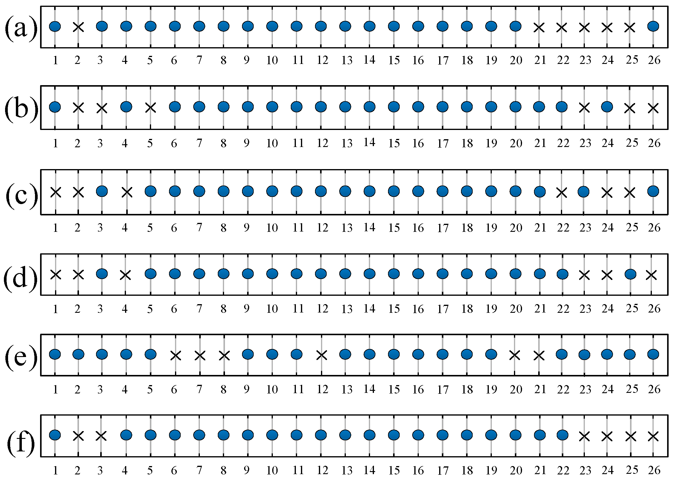
5. Numerical Results

In this section, we evaluate the effectiveness of the proposed method for multiband sparse array design by several numerical experiments. We compare it with other typical algorithms in [21,31]. Specifically, Zheng considered the design of narrowband sparse arrays working at a single frequency under SLL constraint in [21], while Hamza designed a multiband sparse array without SLL control in [31]. It is worth pointing out that Zheng’s and Hamza’s methods cannot tackle the proposed problem (12) since Zheng’s method is only applicable to the single frequency sparse array design while Hamza’s method has no capability of controlling SLL. We only design several different single frequency sparse arrays by using Zheng’s method and a multiband sparse array without SLL control by using Hamza’s method as a benchmark. In fact, the proposed problem has less DoFs than Zheng’s and Hamza’s problems since it is limited by more constraints. In comparison with the proposed problem, Zheng’s problem does not impose restrictions on the sparse weights of all single frequency arrays locating at the same antenna location, while Hamza’s problem has no constraint on the SLLs. Therefore, from the perspective of system DoFs, the performance of the proposed problem would naturally not exceed those of Zheng’s and Hamza’s problems. However, thanks to the adopted solving scheme, the performance of the proposed method may be close to or even better than that of Zheng’s method or Hamza’s method, which is displayed in the following experiments.

In the experiments, the multiband array has the capability of effectively working at $M=4$ frequencies, ${\omega }_1={\omega }_M$, ${\omega }_2=0.972{\omega }_M$, ${\omega }_3=0.944{\omega }_M$, and ${\omega }_4=0.931{\omega }_M$, respectively, where the maximum frequency is ${\omega }_M=3.6\mathrm{GHz}$, which is commonly used in $5\mathrm{G}$ communications and emerging integrated sensing and communication systems. We select $K=20$ antennas from a uniform linear array with $N=26$ locations. For the proposed algorithm, we set $\mu =0.01$, $\epsilon =5\times {10}^{-4}$, and ${\delta }_i=-20\mathrm{dB}$ for all four frequencies. We assume the desired source is located at the direction $80°$ and three interference sources are located at the directions $10°$, $120°$, and $140°$, respectively. The $\mathrm{SNR}$ of the desired source is $0\mathrm{dB}$ and the $\mathrm{INR}$ of each interference source is $40\mathrm{dB}$.

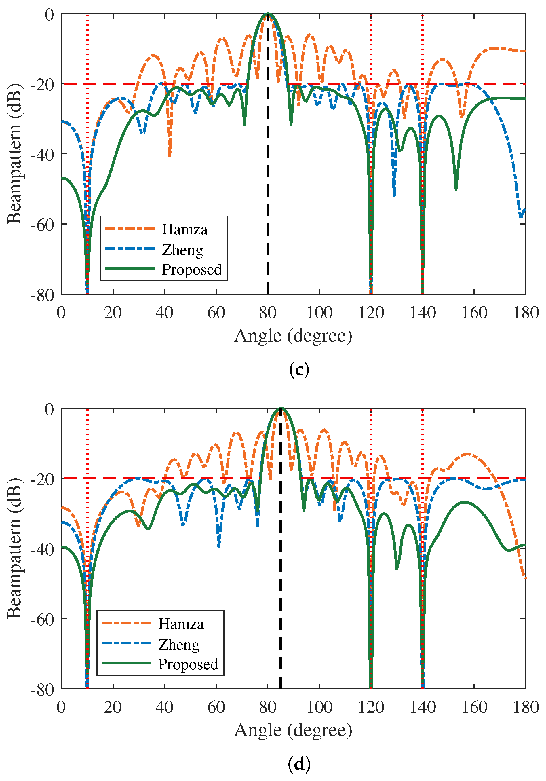
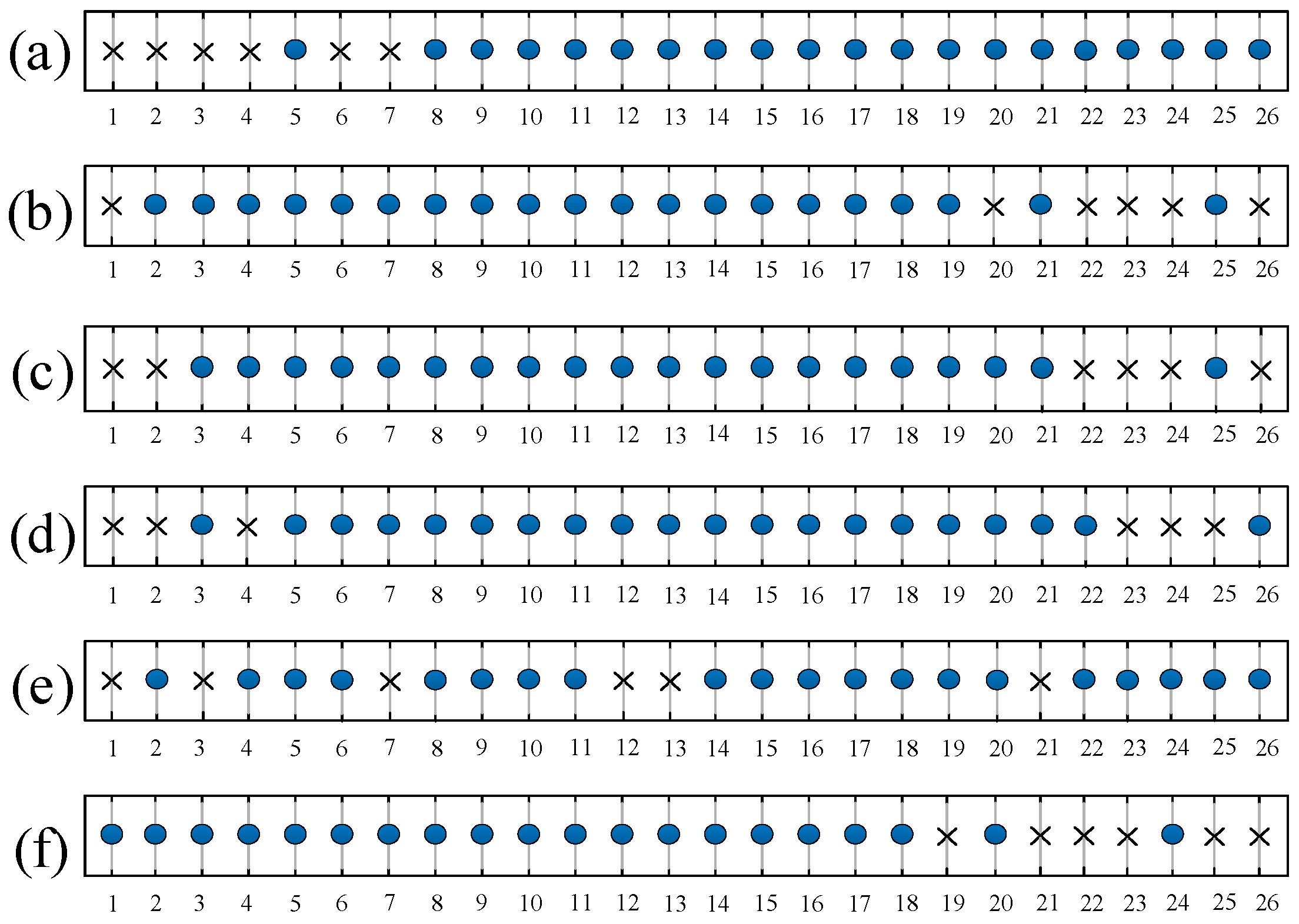
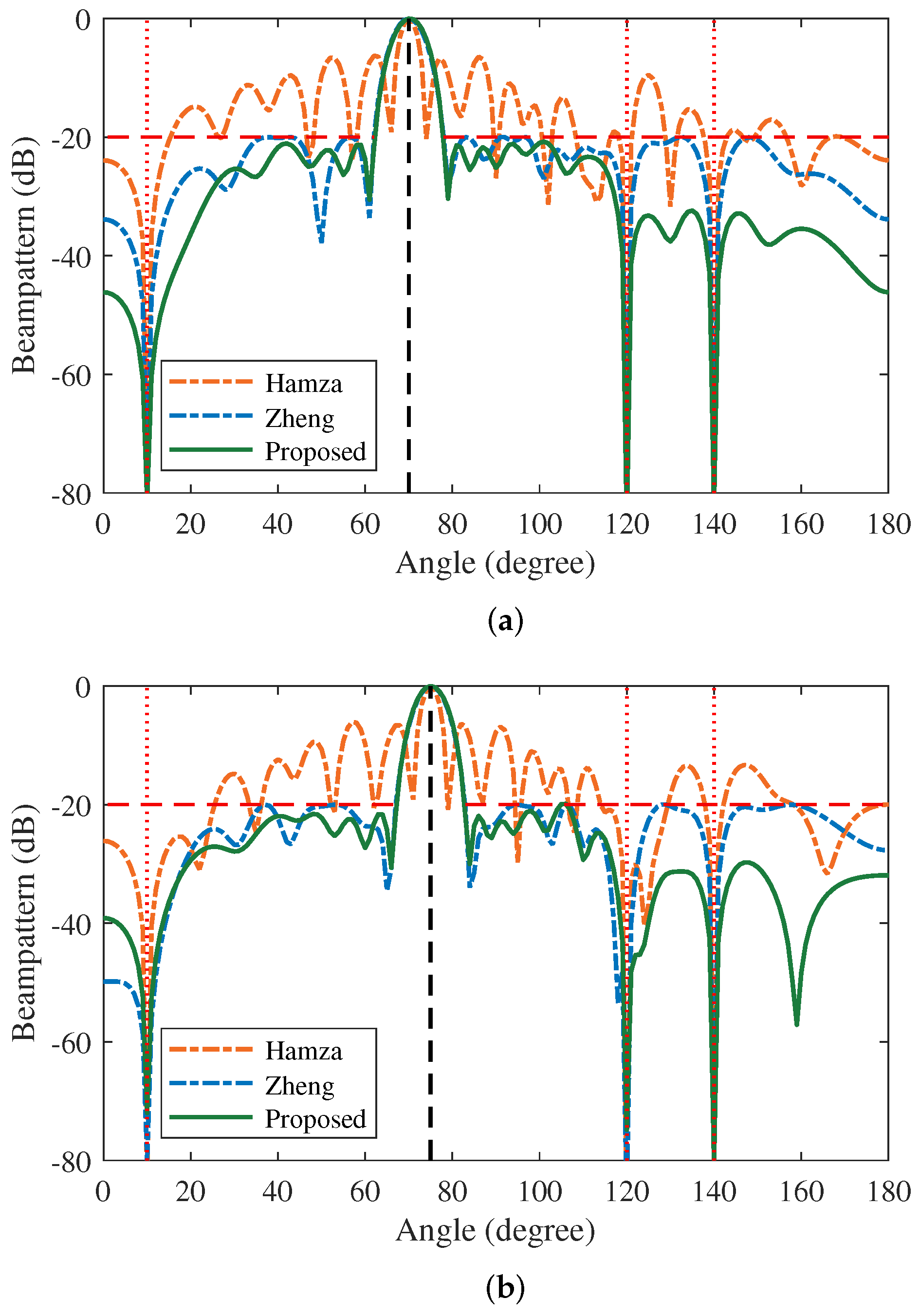
5.1. Beamforming with Multiple Interferences at the Same Desired DOA

Since Zheng’s method can only design a narrowband sparse array working at a single frequency, four optimal narrowband sparse arrays are independently designed at different frequencies, which are provided in Figure 1a–d. On the contrary, Hamza’s method provides a multiband sparse array directly, and its optimal sparse array is shown in Figure 1e. The multiband sparse array obtained by the proposed method is illustrated in Figure 1f. As seen in Figure 2, all three methods form deep nulls at the directions of three interference sources, and thus effectively suppress the interference. Due to the lack of consideration for the sidelobe suppression in Hamza’s method, its SLL is significantly higher than that in Zheng’s method and the proposed one. The proposed method has almost the same SLLs as Zheng’s method. That is to say, compared with Hamza’s method, the proposed method and Zheng’s method will be less sensitive to unknown sporadic interference and thus have superior capability of interference suppression. The null depths of all three methods at each frequency are shown in

Table 1. Null depths (dB) of the three methods at each frequency for the experiment 5.1.

Hamza’s method
	Frequency	${\omega }_1$	${\omega }_2$	${\omega }_3$	${\omega }_4$
Interference
$10°$		−83.60	−83.60	−83.22	−77.56
$120°$		−74.35	−74.35	−75.84	−74.58
$140°$		−87.38	−87.38	−88.64	−82.39
Zheng’s method
	Frequency	${\omega }_1$	${\omega }_2$	${\omega }_3$	${\omega }_4$
Interference
$10°$		−80.88	−75.81	−74.66	−78.79
$120°$		−79.05	−78.02	−81.36	−84.77
$140°$		−82.02	−82.50	−77.95	−82.41
Proposed method
	Frequency	${\omega }_1$	${\omega }_2$	${\omega }_3$	${\omega }_4$
Interference
$10°$		−79.33	−62.62	−84.10	−72.68
$120°$		−76.67	−61.02	−79.84	−68.79
$140°$		−75.59	−59.63	−78.29	−66.52

. In general, we find that the proposed method has a weakly shallower null than Zheng’s and Hamza’s methods, but it is still deep enough to effectively suppress the interferences. From

Table 2. Output SINR (dB) of the three methods at each frequency for the experiment 5.1.

Frequency	${\mathit{\omega }}_1$	${\mathit{\omega }}_2$	${\mathit{\omega }}_3$	${\mathit{\omega }}_4$
Hamza’s method	11.22	11.74	11.55	11.20
Zheng’s method	11.93	13.07	12.59	12.17
Proposed	11.78	10.34	12.07	11.77

, we observe that the proposed method has better output $\mathrm{SINR}$s performance than Hamza’s method and is slightly inferior to Zheng’s method. It is worth pointing out that Zheng’s method is actually the performance upper bound of the multiband sparse array design because it is not constrained by the consistency of antenna locations at each frequency and thus owns more DoFs of antenna selection.

5.2. Beamforming with Multiple Interferences at the Distinct Desired DOAs

In multi-functional communication or radar systems, we also need to receive the desired signals in each frequency band with different DOAs, such as multi-user communications and multiband radars. In this experiment, we therefore set the mainlobe of each frequency with distinct DOAs. From ${\omega }_1$ to ${\omega }_4$, the desired directions are set sequentially as $70°$, $75°$, $80°$, and $85°$, while the sidelobes are correspondingly set as ${\mathsf{\Theta }}_{SL,1}=[0°,62°]\cup [78°,180°]$, ${\mathsf{\Theta }}_{SL,2}=[0°,67°]\cup [83°,180°]$, ${\mathsf{\Theta }}_{SL,3}=[0°,72°]\cup [88°,180°]$, and ${\mathsf{\Theta }}_{SL,4}=[0°,77°]\cup [93°,180°]$. The other parameters are set to be the same as in Section 5.1. The antenna selection results are shown in Figure 3, the normalized receive beampatterns of sparse arrays are displayed in Figure 4, and the null depths at each frequency are shown in

Table 3. Null depths (dB) of the three methods at each frequency for the experiment 5.2.

Hamza’s method
	Frequency	${\omega }_1$	${\omega }_2$	${\omega }_3$	${\omega }_4$
Interference
$10°$		−74.14	−84.16	−77.44	−77.22
$120°$		−79.17	−90.14	−87.49	−89.83
$140°$		−77.55	−77.62	−79.92	−80.79
Zheng’s method
	Frequency	${\omega }_1$	${\omega }_2$	${\omega }_3$	${\omega }_4$
Interference
$10°$		−76.50	−80.15	−83.78	−85.28
$120°$		−74.86	−87.93	−82.38	−77.31
$140°$		−77.27	−76.28	−76.92	−90.73
Proposed method
	Frequency	${\omega }_1$	${\omega }_2$	${\omega }_3$	${\omega }_4$
Interference
$10°$		−81.45	−71.98	−77.27	−75.81
$120°$		−86.18	−74.81	−78.34	−93.93
$140°$		−82.68	−80.69	−79.41	−78.29

. It can be observed from Figure 4 that the mainlobe always points to the desired directions for all three methods, and all three methods form deep null in the preset directions of interference sources. From Table 3, we observe that the proposed method yields almost the same null depths as Zheng’s and Hamza’s methods at each frequency. From

Table 4. Output SINR (dB) of the three methods at each frequency for the experiment 5.2.

Frequency	${\mathit{\omega }}_1$	${\mathit{\omega }}_2$	${\mathit{\omega }}_3$	${\mathit{\omega }}_4$
Hamza’s method	11.21	11.28	11.01	11.15
Zheng’s method	12.54	12.33	12.53	11.97
Proposed	12.09	12.11	12.22	11.59

, we can see that the proposed method achieves higher $\mathrm{SINR}$s than Hamza’s method, even though Hamza’s method did not consider the SLL control. The output $\mathrm{SINR}$s of the proposed method are still close to that offered by Zheng’s method. These results reveal that the proposed method is an efficient method for multiband sparse array design.

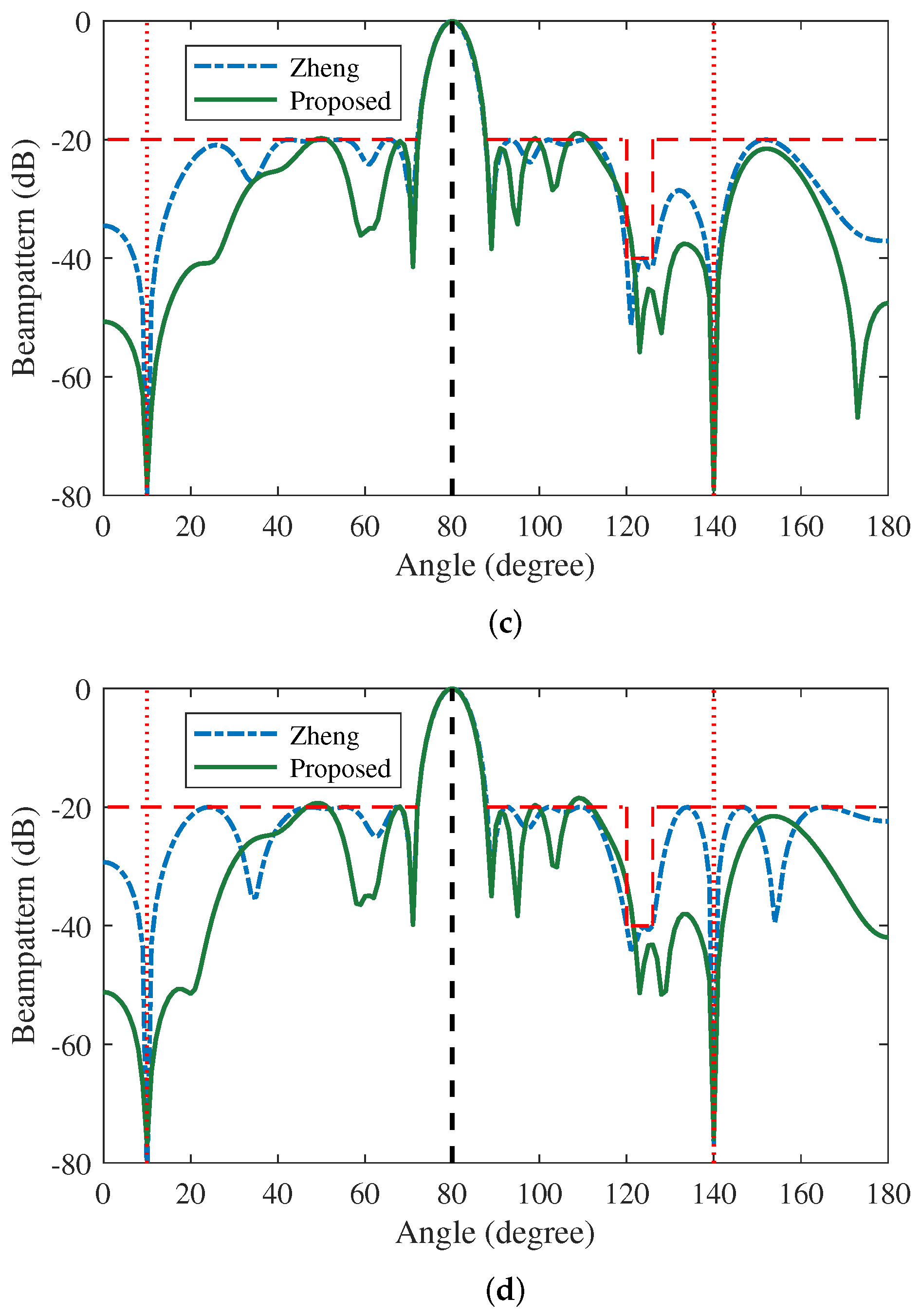
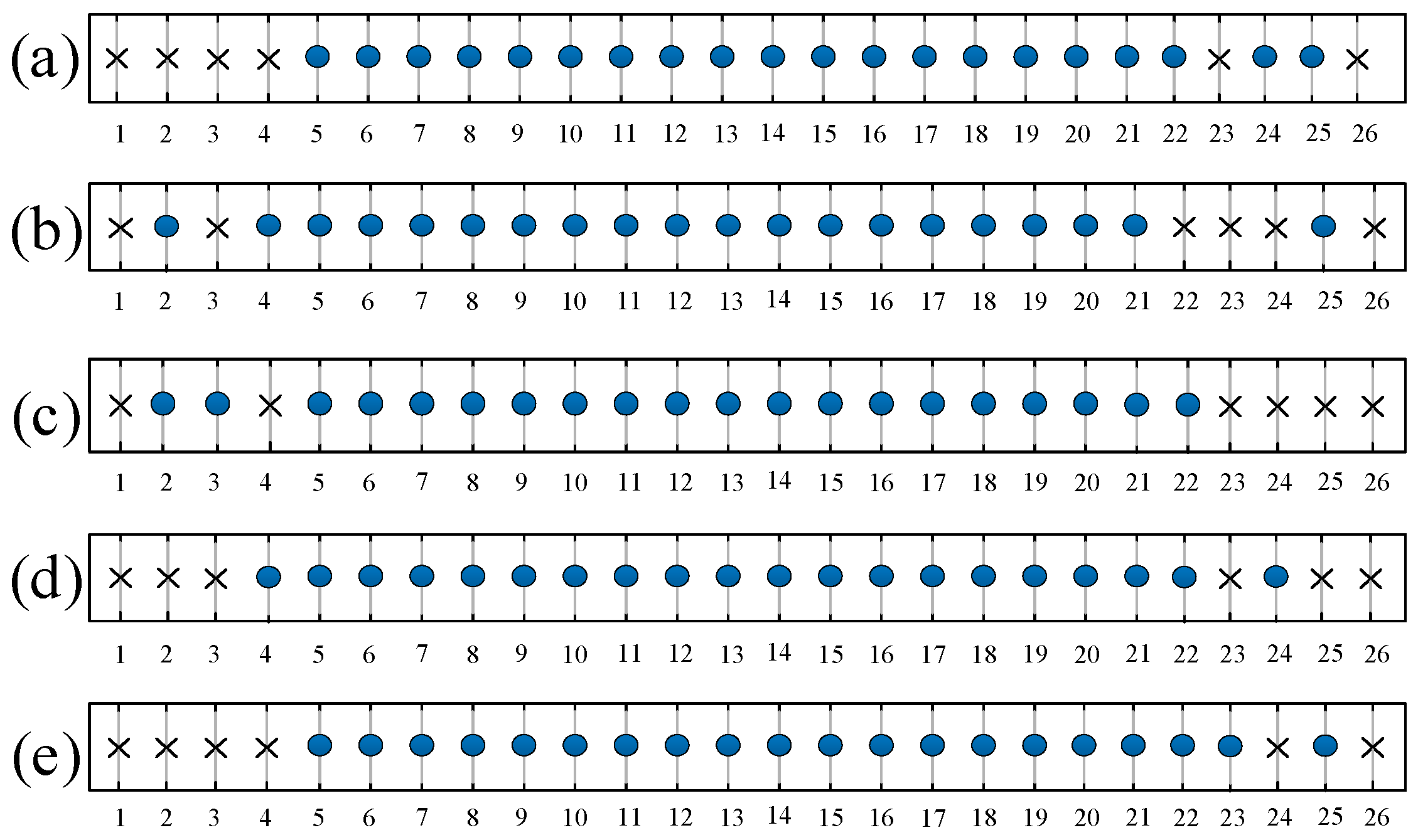
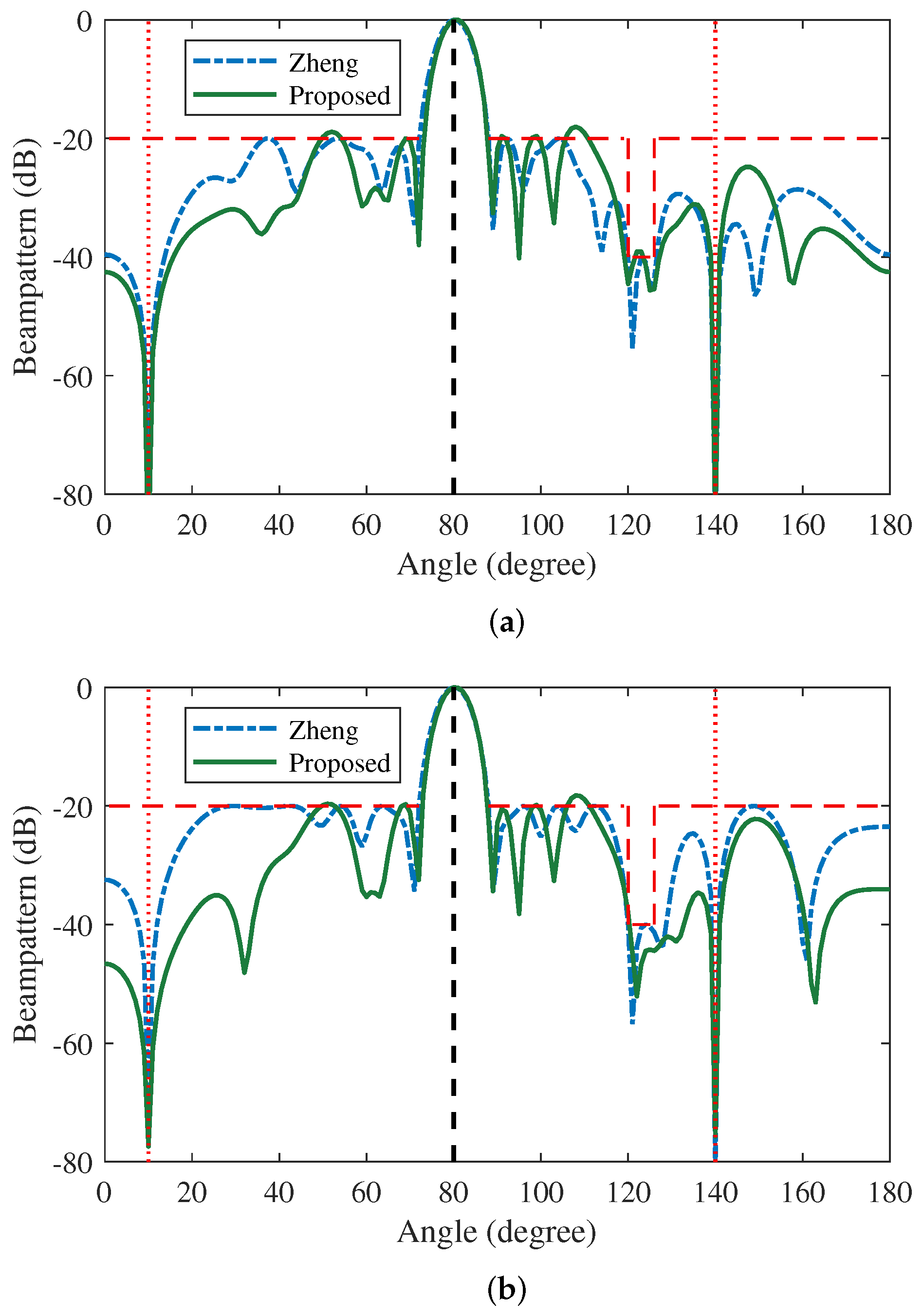
5.3. Nulling Forming at the Same Desired DOA

In real applications, it is often required to generate a deep null region to enhance anti-interference performance at preset directions. In this experiment, we replace the interference source at $120°$ by the null region in $[120°,126°]$ with a null depth of $-40\mathrm{dB}$. As Hamza’s method cannot work in this case, we only demonstrate the results of Zheng’s method and the proposed method. The optimum sparse array configurations are presented in Figure 5. Based on these arrays, Figure 6a–d shows the beampatterns of null forming at the frequencies ${\omega }_1$, ${\omega }_2$, ${\omega }_3$, and ${\omega }_4$, separately.

Table 5. Null depths (dB) of Zheng’s and proposed methods at each frequency for the experiment 5.3.

Zheng’s method
	Frequency	${\omega }_1$	${\omega }_2$	${\omega }_3$	${\omega }_4$
Interference
$10°$		−78.00	−70.18	−79.79	−83.28
$140°$		−85.39	−80.60	−70.88	−76.77
Proposed method
	Frequency	${\omega }_1$	${\omega }_2$	${\omega }_3$	${\omega }_4$
Interference
$10°$		−89.98	−77.42	−78.29	−77.00
$140°$		−85.42	−75.73	−78.98	−75.90

provides the null depths of Zheng’s and the proposed method at each frequency. It can be seen that both the proposed and Zheng’s methods can form a deep null within the preset region $[120°,126°]$ and the interference directions $10°$ and $140°$. Surprisingly, the proposed method generally has lower SLLs than Zheng’s method in the whole sidelobe region. As seen from

Table 6. Output SINR (dB) of Zheng’s and proposed methods at each frequency for the experiment 5.3.

Frequency	${\mathit{\omega }}_1$	${\mathit{\omega }}_2$	${\mathit{\omega }}_3$	${\mathit{\omega }}_4$
Zheng’s method	12.43	12.35	11.97	12.11
Proposed	12.31	11.78	11.71	12.07

, the output $\mathrm{SINR}$s of the proposed method are also close to that of Zheng’s method at all frequencies, even though the constraints become stringent, which further validates the efficiency of the proposed method.

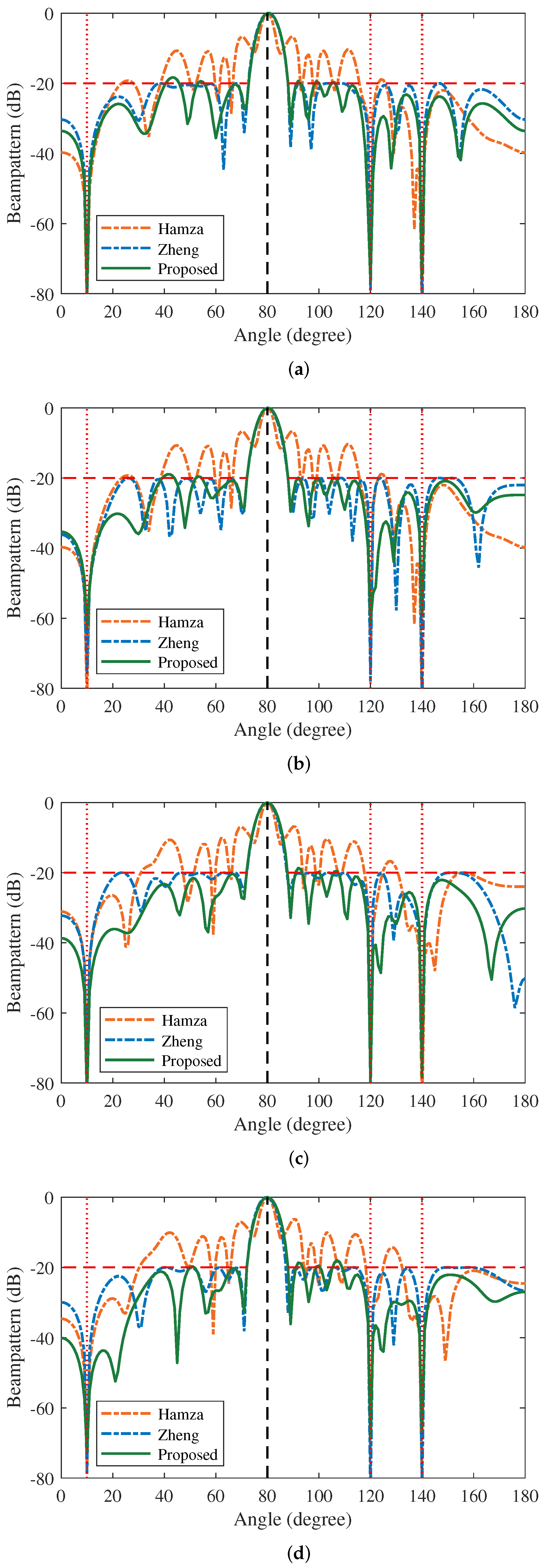
5.4. Nulling Anti-Interference Performance

In order to verify the interference suppression performance of the deep null in the proposed method and Zheng’s method, we add an interference source at the angle direction $122°$ or $124°$ in the null region, respectively. With the same parameters as in Section 5.3, the $\mathrm{INR}$ of this interference source varies from $0\mathrm{dB}$ to $40\mathrm{dB}$, and the variation of the output $\mathrm{SINR}$s are respectively shown in Figure 7a,b. It can be observed from Figure 7 that after adding an interference source into the null region, the $\mathrm{SINR}$ does not change greatly as a whole compared with the null region without an interference source. We can conclude that the increasing $\mathrm{INR}$ of the interference source has a weak effect on the output $\mathrm{SINR}$, which means that both the proposed method and Zheng’s method have the capability of suppressing interference effectively in the null region.

6. Discussion

Traditional sparse array designs for adaptive beamforming are usually discussed in the narrowband case or the wideband case. The multiband sparse array design is an emerging topic due to the rapid development of multi-functional communication and radar systems. Different from narrowband and wideband sparse arrays, the multiband sparse array has some unique characteristics, such as a large frequency gap between two adjacent operating frequencies and different desired source and/or interference directions at each operating frequency. Due to the group sparse regularization of beamforming weights at all operating frequencies, there exists a strong mutual coupling among all beamforming weights, and the objective function or constraints are necessarily nonconvex. On the other hand, the maximum SINR criterion often yields nonconvex quadratic equality constraints to fix the gain of desired directions at each operating frequency. Moreover, if we consider the SLL control, the SLL constraints are also nonconvex because they are the fractional quadratic functions of the beamforming weights. Therefore, the multiband sparse array design is commonly formulated into a complicated nonconvex constrained optimization problem, and its essence is how to effectively solving this problem.

This paper mainly employs several different kinds of convex relaxation techniques to tackle the problem (12), even though it uses the iterative reweighting scheme to promote the group sparse performance. From the perspective of optimization, the relaxation of constraints means that the constraints become more strict and thus the feasible set correspondingly becomes smaller. Therefore, the optimized sparse array of (22) is not necessarily the optimal sparse array of problem (12). Actually, SDR is a somewhat overly strict relaxation technique. To improve the performance of multiband sparse array design, we should utilize other loose relaxation techniques, such as SCA, the convex–concave procedure, and majorization–minimization, or we should handle problem (12) directly by using prevalent nonconvex optimization approaches, involving ADMM, quadratically constrained quadratic programming, and proximal operator algorithms.

7. Conclusions

This paper provided a multiband spare array design method for adaptive receive beamforming with SLL control. With the maximum SINR criterion and SLL constraints, we formulated the proposed joint design of antenna selection and adaptive beamformer as a group sparsity-regularized nonconvex constrained optimization problem. To deal with this intractable problem, we first translated the $l_{0,2}$-mixed norm regularization into a series of reweighted $l_{1,\infty }$-norm regularizations by employing the iterative reweighting technique. We then converted the $l_{1,\infty }$-norm regularized nonconvex optimization problem into the corresponding convex problem by using SDR and linear fractional SDR schemes. With the assistance of the iterative reweighting and SDR, we established the proposed SDR-based iterative reweighted algorithm. We also analyzed the computational complexity of the proposed algorithm. The numerical results verified that the proposed sparse array substantially reduces the SLL in all operating frequencies while maintaining the maximum output SINR performance at the same time, and its performance is approximate to the optimal sparse array designed separately at each frequency.

References

1. He, X.Y.; Chang, L.; Chen, L.L. A multifunction broad-beam antenna with dual bands and dual circular-polarizations. In Proceedings of the 2016 IEEE MTT-S International Wireless Symposium (IWS), Shanghai, China, 14–16 March 2016; pp. 1–4. [Google Scholar] [CrossRef]
2. Sanad, M.; Antennas, A.; Hassan, N. A Multi-band Antenna Configuration for MIMO WiMax in Multi-standard Multifunction Handsets. In Proceedings of the 2009 IEEE Mobile WiMAX Symposium, Napa Valley, CA, USA, 9–10 July 2009; pp. 195–200. [Google Scholar] [CrossRef]
3. Haider, N.; Caratelli, D.; Yarovoy, A.G. Recent Developments in Reconfigurable and Multiband Antenna Technology. Int. J. Antennas Propag. 2013, 2013, 869170. [Google Scholar] [CrossRef]
4. Li, Y.; Sim, C.Y.D.; Luo, Y.; Yang, G. Multiband 10-Antenna Array for Sub-6 GHz MIMO Applications in 5-G Smartphones. IEEE Access 2018, 6, 28041–28053. [Google Scholar] [CrossRef]
5. Moffet, A. Minimum-redundancy linear arrays. IEEE Trans. Antennas Propag. 1968, 16, 172–175. [Google Scholar] [CrossRef]
6. Pal, P.; Vaidyanathan, P.P. Nested Arrays: A Novel Approach to Array Processing with Enhanced Degrees of Freedom. IEEE Trans. Signal Process. 2010, 58, 4167–4181. [Google Scholar] [CrossRef]
7. Vaidyanathan, P.P.; Pal, P. Sparse sensing with co-prime samplers and arrays. IEEE Trans. Signal Process. 2010, 59, 573–586. [Google Scholar] [CrossRef]
8. Zhou, C.; Gu, Y.; He, S.; Shi, Z. A Robust and Efficient Algorithm for Coprime Array Adaptive Beamforming. IEEE Trans. Veh. Technol. 2018, 67, 1099–1112. [Google Scholar] [CrossRef]
9. Zheng, Z.; Yang, T.; Wang, W.Q.; Zhang, S. Robust adaptive beamforming via coprime coarray interpolation. Signal Process. 2020, 169, 107382. [Google Scholar] [CrossRef]
10. Nai, S.E.; Ser, W.; Yu, Z.L.; Chen, H. Beampattern Synthesis for Linear and Planar Arrays with Antenna Selection by Convex Optimization. IEEE Trans. Antennas Propag. 2010, 58, 3923–3930. [Google Scholar] [CrossRef]
11. Wang, X.; Zhai, W.; Zhang, X.; Wang, X.; Amin, M.G. Enhanced Automotive Sensing Assisted by Joint Communication and Cognitive Sparse MIMO Radar. IEEE Trans. Aerosp. Electron. Syst. 2023, 59, 4782–4799. [Google Scholar] [CrossRef]
12. Fuchs, B. Synthesis of Sparse Arrays with Focused or Shaped Beampattern via Sequential Convex Optimizations. IEEE Trans. Antennas Propag. 2012, 60, 3499–3503. [Google Scholar] [CrossRef]
13. Nongpiur, R.C.; Shpak, D.J. Synthesis of Linear and Planar Arrays with Minimum Element Selection. IEEE Trans. Signal Process. 2014, 62, 5398–5410. [Google Scholar] [CrossRef]
14. Fuchs, B.; Rondineau, S. Array Pattern Synthesis with Excitation Control via Norm Minimization. IEEE Trans. Antennas Propag. 2016, 64, 4228–4234. [Google Scholar] [CrossRef]
15. Liang, J.; Zhang, X.; So, H.C.; Zhou, D. Sparse Array Beampattern Synthesis via Alternating Direction Method of Multipliers. IEEE Trans. Antennas Propag. 2018, 66, 2333–2345. [Google Scholar] [CrossRef]
16. Wang, X.; Aboutanios, E.; Amin, M.G. Thinned Array Beampattern Synthesis by Iterative Soft-Thresholding-Based Optimization Algorithms. IEEE Trans. Antennas Propag. 2014, 62, 6102–6113. [Google Scholar] [CrossRef]
17. Oliveri, G.; Massa, A. Bayesian Compressive Sampling for Pattern Synthesis with Maximally Sparse Non-Uniform Linear Arrays. IEEE Trans. Antennas Propag. 2011, 59, 467–481. [Google Scholar] [CrossRef]
18. Hamza, S.A.; Amin, M.G. Hybrid Sparse Array Beamforming Design for General Rank Signal Models. IEEE Trans. Signal Process. 2019, 67, 6215–6226. [Google Scholar] [CrossRef]
19. Zheng, Z.; Fu, Y.; Wang, W.Q. Sparse Array Beamforming Design for Coherently Distributed Sources. IEEE Trans. Antennas Propag. 2021, 69, 2628–2636. [Google Scholar] [CrossRef]
20. Huang, H.; So, H.C.; Zoubir, A.M. Sparse Array Beamformer Design via ADMM. In Proceedings of the 2022 IEEE 12th Sensor Array and Multichannel Signal Processing Workshop (SAM), Trondheim, Norway, 20–23 June 2022; pp. 336–340. [Google Scholar] [CrossRef]
21. Zheng, Z.; Fu, Y.; Wang, W.Q.; So, H.C. Sparse Array Design for Adaptive Beamforming via Semidefinite Relaxation. IEEE Signal Process. Lett. 2020, 27, 925–929. [Google Scholar] [CrossRef]
22. Wang, X.; Greco, M.S.; Gini, F. Adaptive Sparse Array Beamformer Design by Regularized Complementary Antenna Switching. IEEE Trans. Signal Process. 2021, 69, 2302–2315. [Google Scholar] [CrossRef]
23. Hamza, S.A.; Amin, M.G. Learning Sparse Array Capon Beamformer Design Using Deep Learning Approach. In Proceedings of the 2020 IEEE Radar Conference (RadarConf20), Florence, Italy, 21–25 September 2020. [Google Scholar] [CrossRef]
24. Hamza, S.A.; Amin, M.G.; Chalise, B.K. Phase-Only Reconfigurable Sparse Array Beamforming Using Deep Learning. In Proceedings of the ICASSP 2022—2022 IEEE International Conference on Acoustics, Speech and Signal Processing (ICASSP), Singapore, 23–27 May 2022. [Google Scholar] [CrossRef]
25. Crocco, M.; Trucco, A. Stochastic and Analytic Optimization of Sparse Aperiodic Arrays and Broadband Beamformers with Robust Superdirective Patterns. IEEE Trans. Audio Speech Lang. Process. 2012, 20, 2433–2447. [Google Scholar] [CrossRef]
26. Liu, Y.; Zhang, L.; Ye, L.; Nie, Z.; Liu, Q.H. Synthesis of Sparse Arrays with Frequency-Invariant-Focused Beam Patterns Under Accurate Sidelobe Control by Iterative Second-Order Cone Programming. IEEE Trans. Antennas Propag. 2015, 63, 5826–5832. [Google Scholar] [CrossRef]
27. Hawes, M.B.; Liu, W. Sparse array design for wideband beamforming with reduced complexity in tapped delay-lines. IEEE/ACM Trans. Audio Speech Lang. Process. 2014, 22, 1236–1247. [Google Scholar] [CrossRef]
28. Trucco, A. Synthesizing wide-band sparse arrays by simulated annealing. In Proceedings of the MTS/IEEE Oceans 2001. An Ocean Odyssey. Conference Proceedings (IEEE Cat. No.01CH37295), Honolulu, HI, USA, 5–8 November 2001; Volume 2, pp. 989–994. [Google Scholar] [CrossRef]
29. Doblinger, G. Optimized design of interpolated array and sparse array wideband beamformers. In Proceedings of the 2008 16th European Signal Processing Conference, Lausanne, Switzerland, 25–29 August 2008; pp. 1–5. [Google Scholar]
30. Hawes, M.B.; Liu, W. Location Optimization of Robust Sparse Antenna Arrays with Physical Size Constraint. IEEE Antennas Wirel. Propag. Lett. 2012, 11, 1303–1306. [Google Scholar] [CrossRef]
31. Hamza, S.A.; Amin, M.G. Sparse Array Beamforming Design for Wideband Signal Models. IEEE Trans. Aerosp. Electron. Syst. 2021, 57, 1211–1226. [Google Scholar] [CrossRef]
32. Hamza, S.A.; Amin, M.G. Sparse Array DFT Beamformers for Wideband Sources. In Proceedings of the 2019 IEEE Radar Conference (RadarConf), Boston, MA, USA, 22–26 April 2019; pp. 1–5. [Google Scholar] [CrossRef]
33. Wei Liu, S.W. Wideband Beamforming: Concepts and Techniques; Wiley: Hoboken, NJ, USA, 2010. [Google Scholar]
34. Liu, Y.; Zhang, L.; Zhu, C.; Liu, Q.H. Synthesis of Nonuniformly Spaced Linear Arrays with Frequency-Invariant Patterns by the Generalized Matrix Pencil Methods. IEEE Trans. Antennas Propag. 2015, 63, 1614–1625. [Google Scholar] [CrossRef]
35. El-Khamy, S.E.; El-Sayed, H.F.; Eltrass, A.S. A new adaptive beamforming of multiband fractal antenna array in strong-jamming environment. Wirel. Pers. Commun. 2022, 126, 285–304. [Google Scholar] [CrossRef]
36. Monzingo, R.A.; Miller, T.W. Introduction to Adaptive Arrays; Scitech Publishing: Tamil Nadu, India, 2004. [Google Scholar]
37. Mehanna, O.; Sidiropoulos, N.D.; Giannakis, G.B. Joint Multicast Beamforming and Antenna Selection. IEEE Trans. Signal Process. 2013, 61, 2660–2674. [Google Scholar] [CrossRef]
38. Joshi, S.; Boyd, S. Sensor selection via convex optimization. IEEE Trans. Signal Process. 2008, 57, 451–462. [Google Scholar] [CrossRef]
39. Candes, E.J.; Wakin, M.B.; Boyd, S.P. Enhancing sparsity by reweighted l1 minimization. J. Fourier Anal. Appl. 2008, 14, 877–905. [Google Scholar] [CrossRef]
40. Luo, Z.Q.; Ma, W.K.; So, A.M.C.; Ye, Y.; Zhang, S. Semidefinite Relaxation of Quadratic Optimization Problems. IEEE Signal Process. Mag. 2010, 27, 20–34. [Google Scholar] [CrossRef]
41. Karipidis, E.; Sidiropoulos, N.D.; Luo, Z.Q. Quality of Service and Max-Min Fair Transmit Beamforming to Multiple Cochannel Multicast Groups. IEEE Trans. Signal Process. 2008, 56, 1268–1279. [Google Scholar] [CrossRef]
Figure 1. Sparse array configurations for the experiment 5.1, N = 26 , K = 20 . (a) Zheng’s method for ω 1 . (b) Zheng’s method for ω 2 . (c) Zheng’s method for ω 3 . (d) Zheng’s method for ω 4 . (e) Hamza’s method. (f) Proposed method. (Dots mean selected antennas while crosses mean discarded antennas).
Remotesensing 15 04929 g001
Figure 2. Normalized receive beampatterns of sparse arrays in Figure 1a–f at four different frequencies. (a) ω 1 . (b) ω 2 . (c) ω 3 . (d) ω 4 .
Remotesensing 15 04929 g002
Figure 3. Sparse array configurations for the experiment 5.2, N = 26 , K = 20 . (a) Zheng’s method for ω 1 . (b) Zheng’s method for ω 2 . (c) Zheng’s method for ω 3 . (d) Zheng’s method for ω 4 . (e) Hamza’s method. (f) Proposed method. (Dots mean selected antennas while crosses mean discarded antennas).
Remotesensing 15 04929 g003
Figure 4. Normalized receive beampatterns of sparse arrays in Figure 3a–f at four different frequencies. (a) ω 1 . (b) ω 2 . (c) ω 3 . (d) ω 4 .
Remotesensing 15 04929 g004aRemotesensing 15 04929 g004b
Figure 5. Sparse array configurations for the experiment 5.3, N = 26 , K = 20 . (a) Zheng’s method for ω 1 . (b) Zheng’s method for ω 2 . (c) Zheng’s method for ω 3 . (d) Zheng’s method for ω 4 . (e) Proposed method. (Dots mean selected antennas while crosses mean discarded antennas).
Remotesensing 15 04929 g005
Figure 6. Normalized receive beampatterns of sparse arrays in Figure 5a–e at four different frequencies. (a) ω 1 . (b) ω 2 . (c) ω 3 . (d) ω 4 .
Remotesensing 15 04929 g006aRemotesensing 15 04929 g006b
Figure 7. The output SINR with a varied interference in the nulling. (a) an interference source at 122 ° . (b) an interference source at 124 ° .
Remotesensing 15 04929 g007