Intercomparison of CH₄ Products in China from GOSAT, TROPOMI, IASI, and AIRS Satellites

Abstract

Methane (CH₄) is an important greenhouse as well as a chemically active gas. Accurate monitoring and understanding of its spatiotemporal distribution are crucial for effective mitigation strategies. Nowadays, satellite measurements are widely used for CH₄ studies. Here, we use the CH₄ products from four commonly used satellites (GOSAT, TROPOMI, ARIS, and IASI) during the period from 2018 to 2020 to investigate the spatiotemporal variations of CH₄ in China. In spite of the same target (CH₄) for the four satellites, differences among them exist in terms of the instrument, spectrum, and retrieval algorithm. The GOSAT and TROPOMI CH₄ retrievals use shortwave infrared spectra, with a better sensitivity near the surface, while the IASI and AIRS CH₄ retrievals use thermal infrared spectra, showing a good sensitivity in the mid–upper troposphere but a weak sensitivity in the lower troposphere. The GOSAT and TROPOMI observe high CH₄ concentrations in the east and south and low concentrations in the west and north, which is highly related to the CH₄ emissions. The IASI and AIRS show a more uniform CH₄ distribution over China, which reflects the variation of CH₄ at a high altitude. However, a large discrepancy is observed between the IASI and AIRS despite using a similar retrieval band, e.g., significant differences in the seasonal variations of CH₄ are observed between the IASI and AIRS across several regions in China. This study highlights the CH₄ differences observed by the four satellites in China, and caution must be taken when using these satellite products.

1. Introduction

In 2020, China announced its target to achieve carbon neutrality, aiming to peak its carbon emissions by 2030 and reach net zero carbon emissions by 2060 [1]. Atmospheric methane (CH₄) is the second most abundant long-lived greenhouse gas after carbon dioxide (CO₂), with an estimated 20-year global warming potential 84–86 times greater than that of CO₂ [2]. CH₄ is also a chemically active gas that significantly affects the atmospheric environment [3]. Reductions in CH₄ emissions are effective in mitigating radiative forcing and, eventually, global warming [4]. Over the past century, the concentration of CH₄ in the atmosphere has more than doubled following the Industrial Revolution. This rapid increase of CH₄ has primarily been caused by the imbalance of CH₄ sources and sinks, with a significant amount of CH₄ emitted by human activities [5]. However, the spatiotemporal variations of CH₄ emissions have not been well understood [6]. For instance, China is a major CH₄ emitter but has not yet compiled its own CH₄ emission inventory [7]. Satellite data are important for emissions, mainly through the top-down method, which is complementary to the bottom-up inventory. Consequently, it is critical to investigate the spatiotemporal variations of atmospheric CH₄ in China to conduct effective emission reduction strategies.

Accurately monitoring atmospheric CH₄ mole fractions is the first step toward achieving the effective mitigation of CH₄ emissions. Several techniques have been developed, such as in situ observation, ground-based remote sensing, and space-borne remote sensing. Among these methods, space-borne remote sensing provides global-coverage data that can be used to detect and quantify point sources and characterize emissions at the regional and national scales for cross-comparing with the reported bottom-up emissions [8,9]. Currently, there are several widely used satellites providing CH₄ measurements, namely, the Greenhouse Gases Observing Satellite (GOSAT), the Tropospheric Monitoring Instrument (TROPOMI), the Infrared Atmospheric Sounding Interferometer (IASI), and the Atmospheric Infrared Sounder (AIRS). Among them, the GOSAT and TROPOMI satellites retrieve the column-averaged dry-air mole fraction of CH₄ (XCH₄) from the shortwave infrared (SWIR) spectra at 1.65 and 2.3 μm, while the IASI and AIRS satellites derive the CH₄ mole fraction from the thermal infrared (TIR) spectra around 8 μm.

Satellite observations were utilized to study the spatiotemporal distribution of CH₄ concentrations and their driving forces in China. Based on the GOSAT measurements, Qin et al. [10] assessed XCH₄ variations in China during 2010–2012, and Lei et al. [11] conducted a preliminary investigation on the variation of CH₄ concentration given the land-use change in northern China. Zhang et al. [7] investigated the spatiotemporal distributions of XCH₄ in China during 2018–2021 using the TROPOMI measurements. As for the AIRS, due to its earlier launch and longer data coverage, there is a greater amount of research related to it [12,13,14,15,16,17]. These studies mainly use the profile data of the AIRS to investigate the spatial and temporal distribution of the CH₄ concentration in the mid-to-upper troposphere, lower troposphere, and near-surface in China. As shown above, the previous studies on atmospheric CH₄ in China mainly focused on one or two satellites, so the differences among the CH₄ products from the four satellites mentioned above have not been thoroughly discussed.

This study aims to comprehensively explore the differences and similarities among the CH₄ products from the GOSAT, TROPOMI, AIRS, and IASI satellites, to better understand the spatiotemporal distribution of CH₄ in China. The paper is structured as follows: The data and method used in this study are described in Section 2. The spatial distributions of the CH₄ concentrations derived from the four satellites in China, as well as the differences among them, are presented in Section 3. Moreover, the CH₄ emission inventory and model results are separately compared to the results of the SWIR and TIR satellites. The temporal variations of the atmospheric CH₄ in China are also discussed in this section. Finally, conclusions are drawn in Section 4.

2. Materials and Methods

2.1. Data

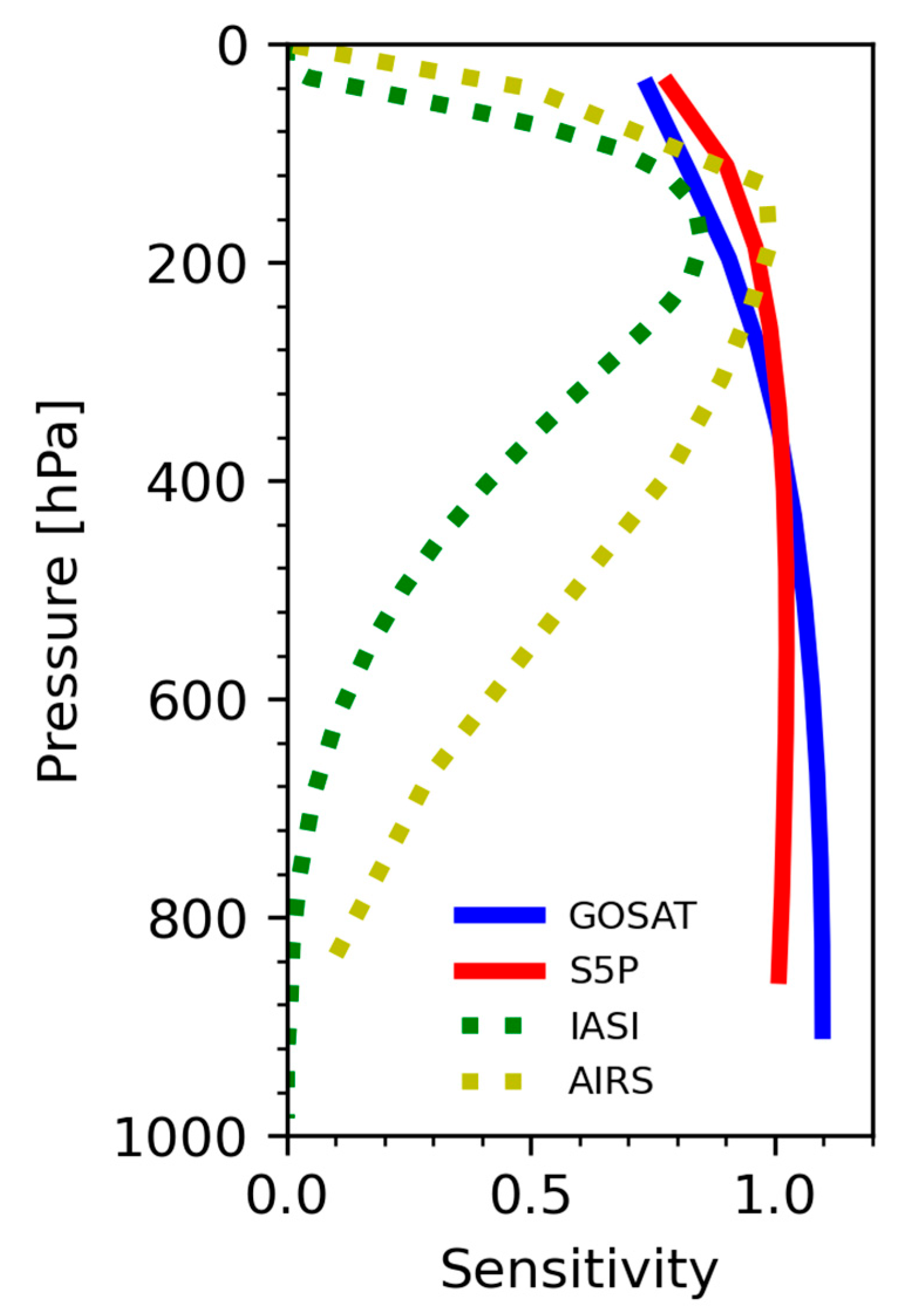
2.1.1. Satellite CH₄ Measurements

Table 1. Satellite instruments for measuring atmospheric CH₄.

Instruments	TANSO-FTS	TROPOMI	IASI	AIRS
Satellite	GOSAT	S5P	MetOp-A	Aqua
Agency	JAXA	ESA, NSO	EUMETSAT	NASA
Data period	2009–now	2017–now	2007–now	2002–now
Overpass time [local time]	01:00/13:00	01:30/13:30	09:30/21:30	01:30/13:30
Fitting window [nm] Spectral resolution	1560–1720 0.27 cm−1	2310–2390 0.25 nm	7100–8300 0.5 cm−1	6200–8200 0.5 cm−1
Pixel size	10.5 km	5.5 × 7.0 km2	12 km	13.5 km
Swath [km]	Discrete, 1–9 points	2600	2200	1650
Reference	Kuze et al. (2009) [18]	Lorente et al. (2021) [19]	Crevoisier et al. (2009) [20]	Xiong et al. (2008) [21]

lists the key characteristics of the four satellites used in this study. SWIR spectra are observed by satellite from the solar radiation reflected by the Earth’s surface and backscattered by its atmosphere. As a result, the GOSAT and TROPOMI CH₄ measurements derived from the SWIR spectra are only available during the daytime. In contrast, TIR signals are emitted by the Earth and its atmosphere and can be detected during both daytime and nighttime. All these satellites are in polar sun-synchronous low-Earth orbits (LEO).

The Thermal And Near infrared Sensor for carbon Observations-Fourier Transform Spectrometer (TANSO-FTS) instrument onboard the GOSAT was developed by the Japan Aerospace Exploration Agency (JAXA) and was launched in January 2009 [22]. It is the first space-based sensor specifically measuring greenhouse gases based on high-resolution SWIR spectra [23,24]. The SRFP (the full-physics of SRON/KIT’s RemoTec Algorithm) of the GOSAT bias-corrected daily L2 XCH₄ measurements (CH₄_GOS_SRFP, v2.3.8) from January 2018 to December 2019 are used in this study. The SRFP adjusts parameters of surface, atmosphere, and satellite instrument to fit the GOSAT spectra [25]. The satellite data are downloaded from the Copernicus climate data center (https://cds.climate.copernicus.eu/, accessed on 30 January 2022). We use the SRFP/GOSAT products as they were developed on the basis of the RemoTeC/TROPOMI algorithm [23].

TROPOMI is the sensor onboard the Sentinel-5 precursor (S5P) satellite, with its daily global coverage at an unprecedented resolution of 7 × 7 km² since its launch in October 2017 (upgraded to 5.5 × 7.0 km² in August 2019). It aims at providing accurate and timely observations of abundances of the atmospheric species, such as CH₄ and CO, for air quality and climate change research and service [26]. The RemoTeC is the S5P operational algorithm for CH₄ at the SWIR bands, which is in essence the same as the SRFP algorithm. It also uses the full-physics approach that simultaneously retrieves the atmospheric CH₄ mole fraction and the physical scattering properties of the atmosphere. In this study, the bias-corrected daily granule XCH₄ products, spanning from January 2018 to December 2020, are provided by ESA (European Space Agency, https://scihub.copernicus.eu/, accessed on 30 January 2022).

IASI onboard the MetOp is a Fourier transform spectrometer that measures infrared radiation. The IASI CH₄ retrieval uses 10 channels around the 7.7 μm spectral region that are mostly sensitive to CH₄ and temperature. The Advanced Microwave Sounding Unit (AMSU) also onboard the MetOp provides microwave observations only sensitive to temperature that can be used to separate the effects of temperature and CH₄. The retrieval algorithm developed at the Centre National de Recherche Scientifique (CNRS)-Laboratoire de Météorologie Dynamique (LMD) is based upon a nonlinear regression inverse radiative transfer model using a multilayer perceptron [20]. The retrieved CH₄ integrated columns are weighted to the mid-to-upper troposphere with peak sensitivity at about 200 hPa (~11 km), half the peak sensitivity at 100 and 300 hPa (~6 and 16 km), and almost no sensitivity at the surface [27]. In this study, the IASI level 2 mid-to-upper tropospheric columns of the atmospheric CH₄ (MUT_CH₄; written as XCH₄ for comparison with other satellites in the following texts) products (CH₄_IASB_NLIS, v9.1) from 2018 to December 2020 are downloaded from https://iasi.aeris-data.fr/catalog/, accessed on 30 January 2022.

AIRS is a nadir cross-track scanning infrared spectrometer, and was launched on 4 May 2002 onboard the EOS/Aqua platform. The AIRS measures approximately 200 channels in the 7.66 μm absorption band of CH₄, of which 71 channels are used to retrieve the CH₄ profile. The atmospheric temperature profile, water vapor profile, surface temperature, surface emissivity, and a priori profile of CH₄ are inputted into a forward model to compute the upwelling radiance. The differences between the computed radiance and the observed clear-sky radiance are used to invert the CH₄ profile [21]. In this study, the AIRS V7 L2 support products (AIRS2RET 7.0) from January 2018 to December 2020 are downloaded from http://disc.sci.gsfc.nasa.gov/, accessed on 30 January 2022. The AIRS2RET 7.0 data provide CH₄ volume mixing ratio (VMR) profiles at 100 levels from 1100 hPa to 0.0161 hPa.

2.1.2. CH₄ Emission Inventory

The CH₄ emissions used in this study are from the Emissions Database for Global Atmospheric Research (EDGAR V6.0, https://edgar.jrc.ec.europa.eu/, accessed on 5 February 2022). EDGAR is a widely used inventory for anthropogenic emissions of greenhouse gases such as CO₂, CH₄, and N₂O, as well as fluorinated gases per sector and country. The EDGAR CH₄ emission data include emissions from energy manufacturing, coal/oil/gas production, agricultural soils, waste disposal, etc. [28]. It has been used as an important reference for many emission-related studies [29]. Moreover, we followed the regional division proposed by Wang et al. (2022) [30] and looked into the four regions specifically in China, namely north-eastern China (NE), south-eastern China (SE), north-western China (NW), and the Qinghai–Tibet Plateau (TP), to further investigate the spatiotemporal variations of CH₄ and the differences among the four satellites. These regions differ in climate, agricultural types, major economic activities, and CH₄ emission sources. Figure 1 illustrates the spatial distribution of CH₄ emissions in China for the year 2018, with a spatial grid of 0.1° × 0.1°, along with the regional division used in this study. It reveals that the SE and NE regions have higher levels of anthropogenic CH₄ emissions, while the TP and NW regions exhibit relatively lower emissions.

2.1.3. CAMS Global Greenhouse Gas Reanalysis (EGG4)

The Copernicus Atmosphere Monitoring Service (CAMS) provides near-real-time analysis and forecast data on atmospheric composition with a globally horizontal resolution of 0.75° × 0.75°. The reanalysis procedure combines model data with satellite data into a globally complete and consistent dataset using the European Centre for Medium-range Weather Forecasts’ Integrated Forecasting System (IFS). The purpose of the CAMS GHG analyses is to provide realistic global 4D fields of the atmospheric CO₂, CH₄, and N₂O mole fractions [31]. This study uses monthly CAMS data, downloaded from https://ads.atmosphere.copernicus.eu/cdsapp#!/dataset/cams-global-ghg-reanalysis-egg4?tab=form, accessed on 5 February 2022, which provides the CH₄ column-mean molar fraction and VMR profiles at 25 vertical levels from 1000 hPa to 1 hPa. The CAMS model assimilates ground-based observations, e.g., NOAA, ICOS in situ measurements, and satellite observations, including the SCIAMCHY, GOSAT and IASI [32]. Note that the CAMS model only assimilates the IASI data in the tropical region, so that the CAMS reanalysis data can be used as an independent reference to compare with the IASI and AIRS above China.

2.2. Methods

In order to compare the AIRS data with other satellites’ products, we convert the AIRS CH₄ VMR profiles to $X{\mathrm{CH}}_4$ as follows

$$X{\mathrm{CH}}_4=\frac{T{C}_{{\mathrm{CH}}_4}}{T{C}_{\mathrm{air}}^{\mathrm{dry}}} ,$$

(1)

$$T{C}_{\mathrm{air}}^{\mathrm{dry}}=\frac{P_{\mathrm{s}}/g-T{C}_{{\mathrm{H}}_2\mathrm{O}}^{\mathrm{m}}}{m_{\mathrm{air}}^{\mathrm{dry}}/N_{\mathrm{a}}} ,$$

(2)

where $T{C}_{{\mathrm{CH}}_4}$ is the total column of CH₄ (molecules/cm²), $P_{\mathrm{s}}$ is the surface pressure, $T{C}_{{\mathrm{H}}_2\mathrm{O}}^{\mathrm{m}}$ is the mass of total column water vapor (kg/m²), $g$ is the column-averaged gravitational acceleration varying with location, $m_{\mathrm{air}}^{\mathrm{dry}}$ is the molecular masses of H₂O, and $N_{\mathrm{a}}$ is the Avogadro constant.

We aggregated all satellite CH₄ data into 0.5° × 0.5° grids and calculated the mean value within each grid to obtain the spatial distribution of CH₄ in China. Note that we only took the data that was of a good quality according to the qa_value or quality_flag given in each product.

Before comparison, it is necessary to look at their respective averaging kernels that represent the vertical sensitivities of the retrieval to the true state. Figure 2 shows the typical averaging kernels of the four satellites. The GOSAT and TROPOMI measurements have a nearly uniform sensitivity close to unity within the troposphere, especially in the lower troposphere, thereby enabling them to efficiently characterize the CH₄ variations in the lower troposphere. The AIRS and IASI have a good sensitivity to the middle-to-upper troposphere (about 200 hPa) but have a weak signal in the lower troposphere. The reason is that the thermal difference between the atmosphere and the surface is not large enough to gain information in the lower troposphere. To conclude, the SWIR instruments (GOSAT and TROPOMI) have good sensitivity in both the troposphere and stratosphere, while the TIR instruments (AIRS and IASI) are mainly sensitive to the CH₄ changes in the upper troposphere and lower stratosphere. As the TROPOMI and GOSAT use almost the same retrieval algorithm and have similar vertical sensitivities, we compared their XCH₄ products directly. Regarding the TIR instruments (IASI and AIRS), their peak sensitivities correspond to a similar altitude (~200 hPa), so we compared the AIRS partial column-averaged mole fraction of CH₄ between 100 hPa and 300 hPa with the IASI XCH₄. Similarly, we compared the CAMS partial column-averaged mole fraction of CH₄ between 100 hPa and 300 hPa with the AIRS and IASI, respectively.

3. Results and Discussion

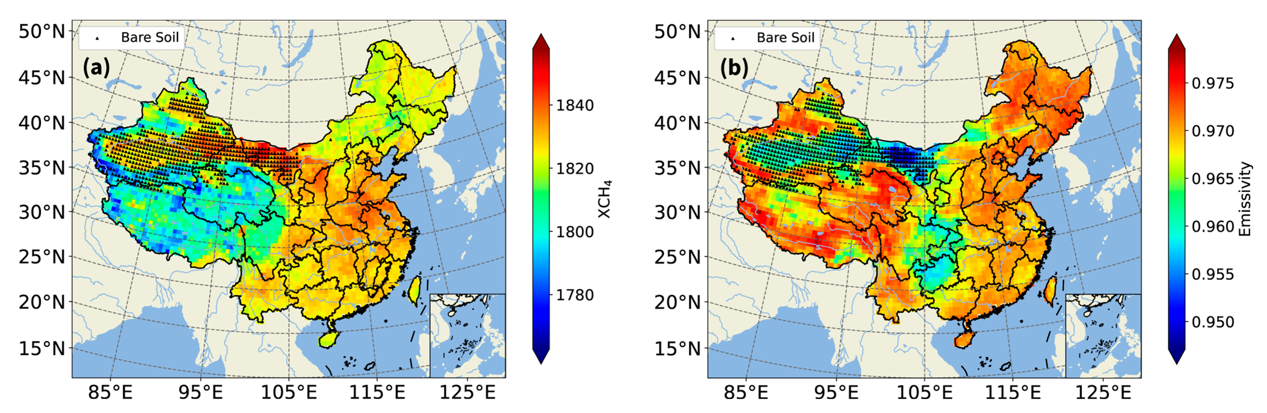
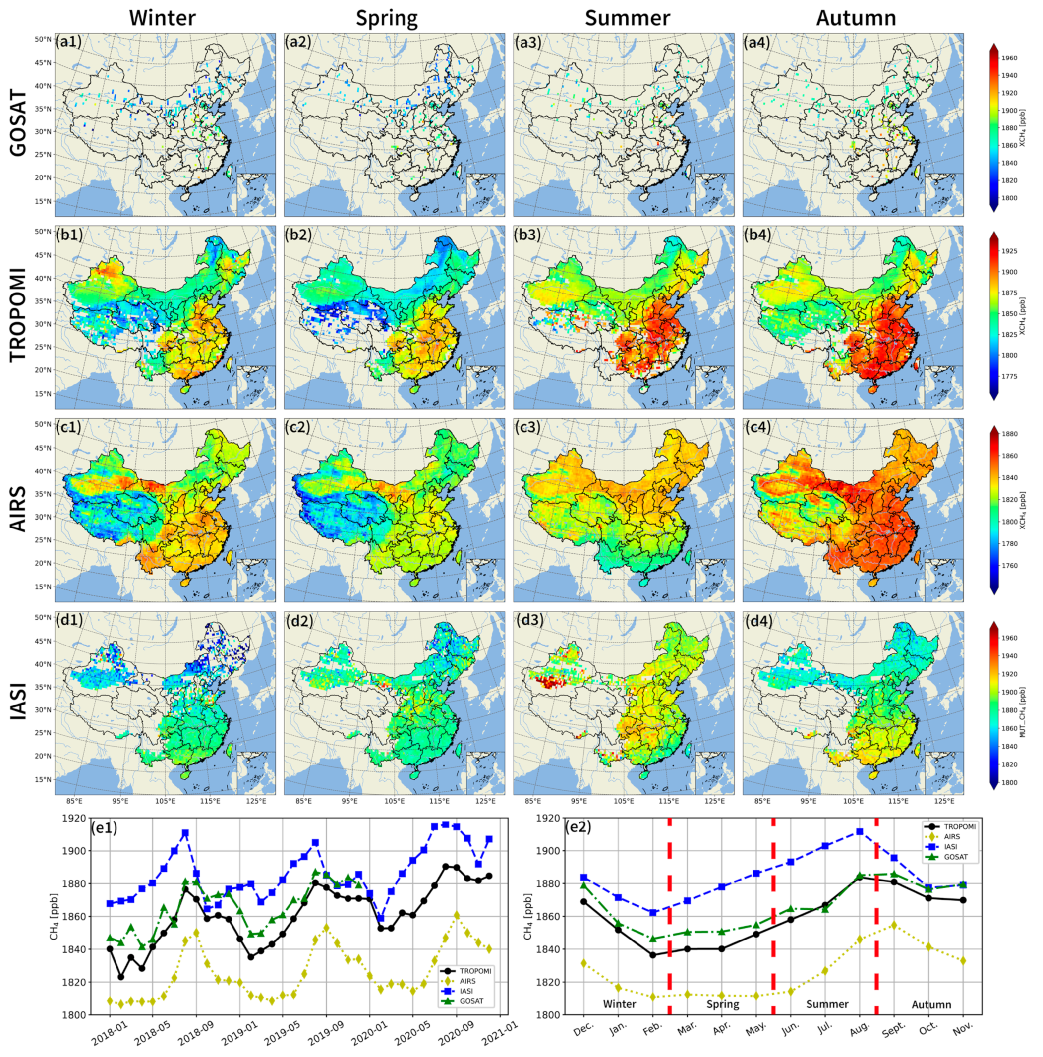
3.1. Spatial Distribution of CH₄ in China

The XCH₄ maps above China observed using the four satellites are shown in Figure 3. Note that the TROPOMI and AIRS have good spatial coverages in China. However, the data density of GOSAT is notably scarce, and the IASI suffers from a significant gap over the Qinghai–Tibet Plateau.

The TROPOMI and GOSAT XCH₄ measurements show a consistent spatial pattern, with higher values in the south and east and lower values in the north and west of China. Compared to the GOSAT, TROPOMI could provide advantages due to its much larger data density. For instance, the TROPOMI XCH₄ measurements can observe XCH₄ hotspots in cities [33,34]. From the TROPOMI XCH₄ map, we can clearly recognize high XCH₄ values in the north, central, and the south of China as well as the Sichuan Basin, and lower XCH₄ values in the Qinghai–Tibet Plateau and northeast China. This spatial distribution of XCH₄ observed from the TROPOMI is highly consistent with the EDGAR anthropogenic emissions (Figure 1).

The spatial distribution of the IASI XCH₄ measurements in China is relatively uniform compared to that of the TROPOMI. The changes in CH₄ concentrations in the mid-upper troposphere are mainly influenced by atmospheric transport and less affected by surface emissions. The IASI measurements show a slight latitude gradient, with higher concentrations in the south and lower values in the north. Nevertheless, the IASI measurements still show a similar CH₄ spatial distribution in China compared to the TROPOMI. However, the AIRS XCH₄ measurements have a different spatial pattern, with the highest values in Inner Mongolia and the northwestern regions. Moreover, the AIRS XCH₄ values are about 30–60 ppb systematically lower than the other three satellites.

It is abnormal to observe high XCH₄ values in NW from the AIRS measurements, as the CH₄ emissions are relatively low in that region (Figure 1). Figure 4 shows these high-value areas, along with a surface emissivity around 1300 cm⁻¹ (~7700 nm) and the bare soil surface type. It was found that the high XCH₄ values in Inner Mongolia and northwestern China correspond to the low emissivity areas. The land surface emissivity in the thermal infrared usually increases when the vegetation amount increases, which has been explained by internal reflection occurring inside of a plant canopy, constituting a “cavity effect” [35]. Therefore, the thermal infrared surface emissivity of bare soil is usually lower than that of vegetation. In addition, the heat capacity of bare soil is smaller than that of vegetation or water, so under the same radiation conditions its temperature changes more significantly, which also affects the surface emissivity. Low surface emissivity leads to a low signal-to-noise ratio of the infrared spectrum, and the AIRS CH₄ retrieval is found to be affected by it.

3.2. Intercomparison between Satellites

3.2.1. Comparison between the GOSAT and TROPOMI Measurements

As shown in Figure 5, the mean and standard deviation of the differences between the TROPOMI and GOSAT (TROPOMI-GOSAT) co-located XCH₄ measurements are −14.2 ± 18.0 ppb in NW, −14.6 ± 19.6 ppb in NE, −13.4 ± 16.3 ppb in TP, and −6.3 ± 14.9 ppb in SE. The correlation coefficients for these regions are 0.71, 0.78, 0.74, and 0.80, respectively. It is worth noting that the number of co-located data points varies across the four regions, with 1082 in NW, 493 in NE, 65 in TP, and 111 in SE. The TROPOMI and GOSAT show good consistency in all four regions, especially in SE, where they have the highest correlation coefficient and the smallest bias and standard deviation. The bias in the NW, NE, and TP regions is approximately 85% higher than that in SE. The XCH₄ of TROPOMI is more affected by the surface albedo compared to the GOSAT [36]. As the NW, NE, and TP regions have higher snow cover than the SE region, this may be the reason for the higher biases [19].

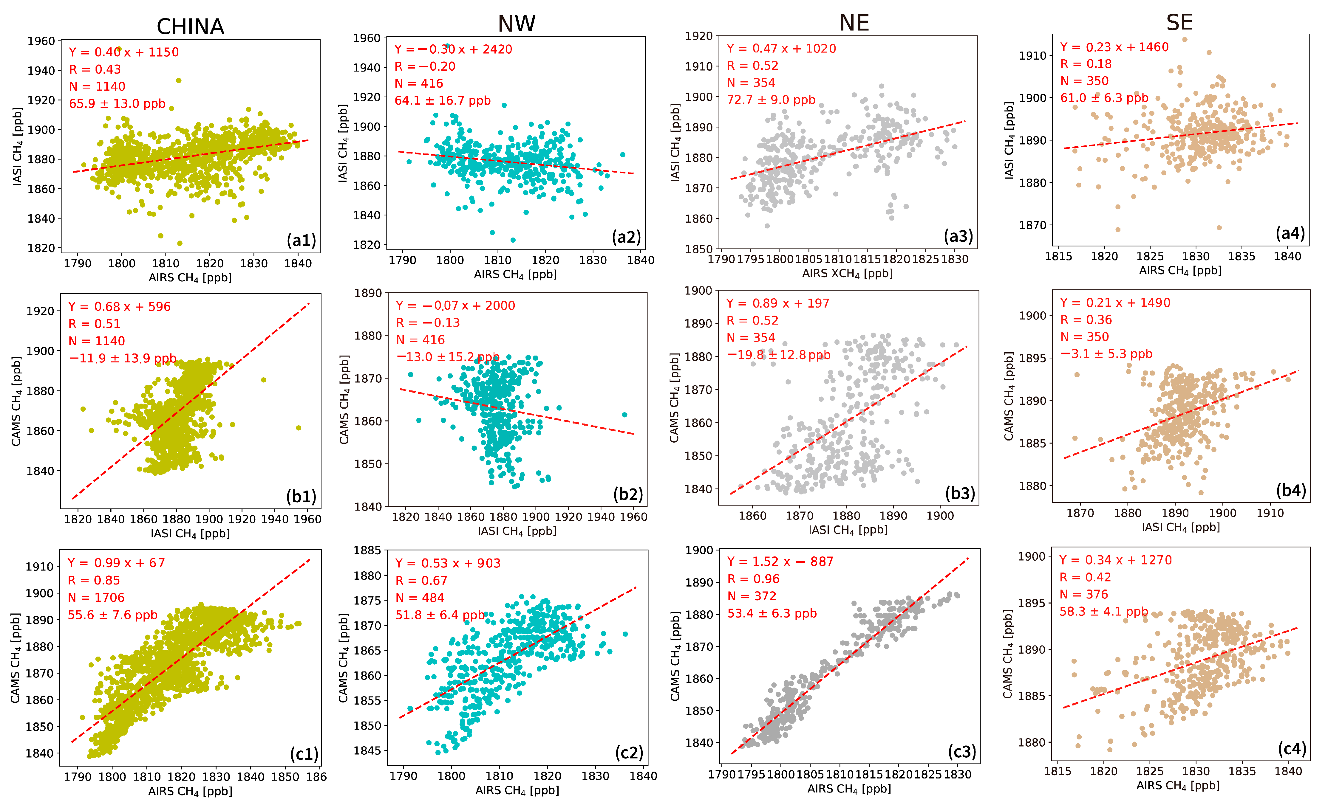
3.2.2. Comparison between the IASI and AIRS Measurements

As the IASI has a significant gap over the Qinghai–Tibet Plateau, we only showed the differences between the IASI and AIRS CH₄ measurements in the NW, NE, and SE regions (of China). As shown in Figure 6(a1–a4), the mean and standard deviation of the differences between the IASI and AIRS (IASI-AIRS) co-located CH₄ measurements are 65.9 ± 12.0 ppb in China, 64.1 ± 16.7 ppb in NW, 72.7 ± 9.0 ppb in NE, and 61.0 ± 6.3 ppb in SE. The IASI CH₄ is systematically higher than the AIRS CH₄. The correlation coefficients for each region are 0.43, −0.20, 0.52, and 0.18, respectively. The region with the best correlation is NE, while the NW and SE regions have poor correlations (R ≤ 0.2).

It is unexpected to find such a large difference between the IASI and AIRS, as they use similar retrieval windows. To further validate the usability of the two products, we used the CAMS model data as an independent dataset to compare with both IASI and AIRS, respectively.

As shown in Figure 6(b1–b4), the mean and standard deviation of the differences between the CAMS and IASI (CAMS-IASI) co-located CH₄ measurements are −11.9 ± 13.9 ppb in China, −13.0 ± 15.2 ppb in NW, −19.8 ± 12.8 ppb in NE, and −3.1 ± 5.3 ppb in SE. The IASI CH₄ is also systematically higher than the CAMS model, but compared to the AIRS, the mean difference has significantly decreased. The correlation coefficients for each region are 0.51, −0.13, 0.52, and 0.36, respectively. Similar to the comparison between the IASI and AIRS, the region with the best correlation between the CAMS and IASI is NE, followed by SE. The NW region exhibits the worst correlation, with a negative value. Figure 6(c1–c4) show that the mean and standard deviation of the differences between the CAMS and AIRS (CAMS-AIRS) co-located CH₄ measurements are 55.6 ± 7.6 ppb in all of China, 51.8 ± 6.4 ppb in NW, 53.4 ± 6.3 ppb in NE, and 58.3 ± 4.1 ppb in SE. The CAMS CH₄ is systematically higher than the AIRS CH₄. Compared to the CAMS-IASI, the bias is higher but the standard deviation is lower. The correlation coefficients for each region are 0.85, 0.67, 0.96, and 0.42, respectively. The CAMS-AIRS demonstrates better correlation coefficients in all regions, with a notable increase observed in NE and NW.

When compared using the CAMS model, the AIRS measurements can better present the CH₄ variation in the mid-upper troposphere compared to the IASI measurements, especially in NE and NW. Since the training dataset of the IASI neural network retrieval algorithm mainly comes from tropical low-latitude regions [20], it might cause a flawed result in high-latitude regions, such as NW. The correlation between the CAMS and AIRS in SE is relatively weak, which is likely due to the impact of the East Asian monsoon on the distribution of CH₄ concentrations in the middle-to-upper troposphere [37,38]. As SE is of importance as a major source of CH₄ emissions in China, further investigation is needed to better understand the distribution of CH₄ concentrations in the middle-to-upper troposphere in this area. For instance, comparing and verifying satellite and model data with aircraft profile observations could enhance the dataset’s reliability.

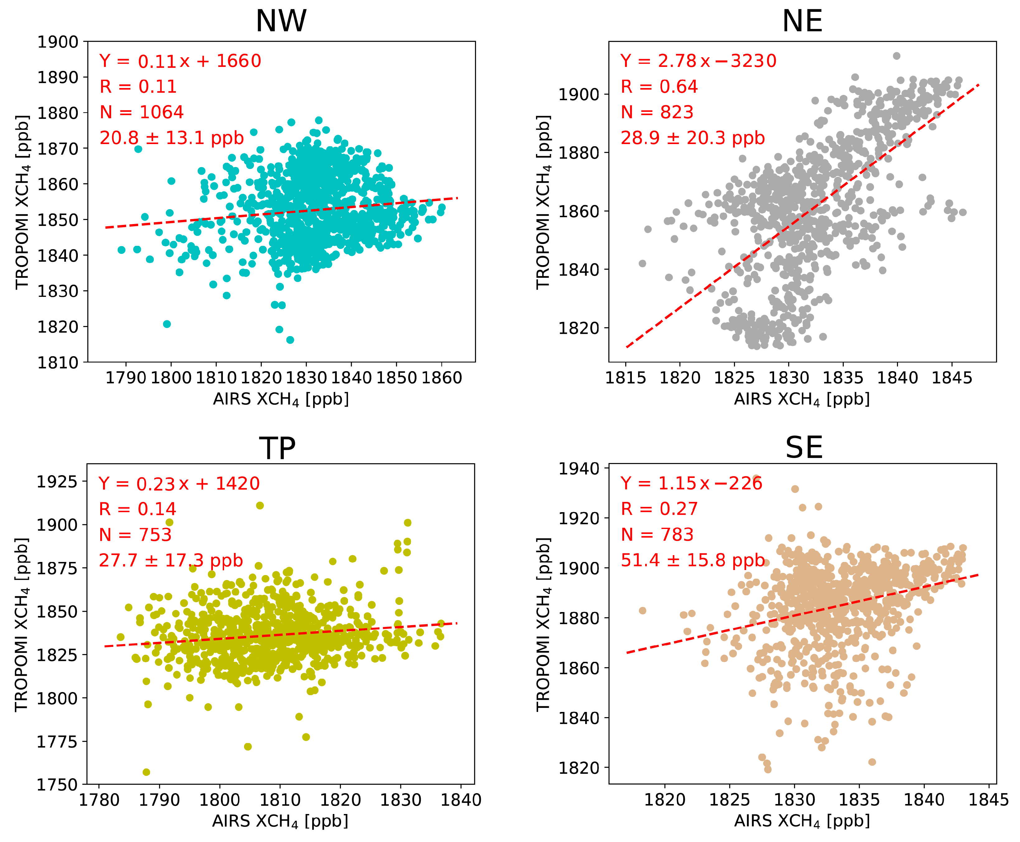
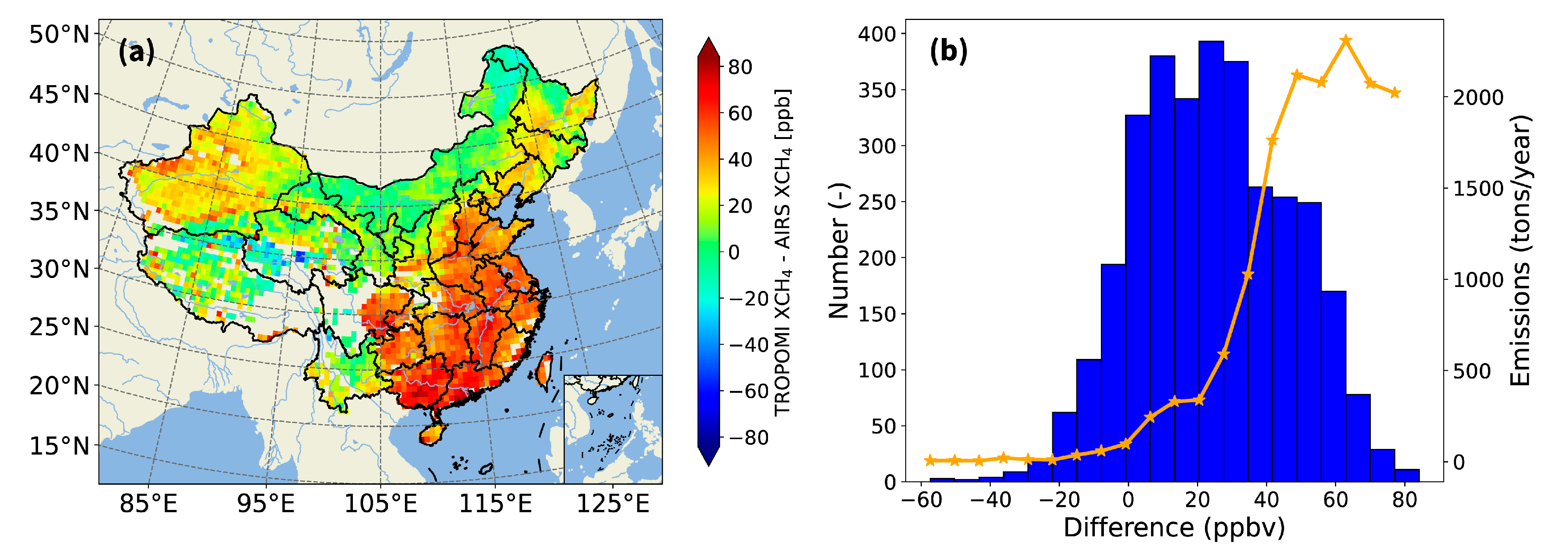
3.2.3. Comparison between the TROPOMI and AIRS Measurements

Here, we highlight the difference between the SWIR and TIR retrievals. Both the SWIR and TIR satellite measurements are widely used in CH₄ research studies, but users might ignore their differences. Figure 7 shows the scatter plots of the TROPOMI and AIRS co-located XCH₄ measurements. The mean and standard deviation between the TROPOMI and AIRS (TROPOMI-AIRS) are 20.8 ± 13.1 ppb in NW, 28.9 ± 20.3 ppb in NE, 27.7 ± 17.3 ppb in TP, and 51.4 ± 15.8 ppb in SE. The TROPOMI XCH₄ is systematically higher than the AIRS XCH₄, which is also consistent with the IASI and CAMS data. These results confirm that the AIRS XCH₄ is systematically underestimated. The correlation between the TROPOMI and AIRS is relatively high in NE (R = 0.64), while pretty weak in the other regions (NW: R = 0.11; TP: R = 0.14; SE: R = 0.27).

The spatial distribution of the differences between the TROPOMI and AIRS XCH₄ is shown in Figure 8a, which has a similar pattern to the CH₄ anthropogenic emissions (Figure 1). Figure 8b demonstrates the frequency histogram of the XCH₄ differences along with absolute CH₄ emissions. It is found that large positive differences between the two XCH₄ datasets correspond to strong CH₄ emissions. The difference between the TROPOMI and AIRS is up to 80 ppb in SE, where the largest CH₄ emission exists. The AIRS CH₄ retrievals are mainly sensitive to the middle-to-upper troposphere, but less sensitive to the lower troposphere. Therefore, the AIRS CH₄ retrieval in the lower troposphere relies heavily on the a priori profiles.

Based on the optimal estimation method

$$x_{\mathrm{r},\mathrm{T}}=x_{\mathrm{a},\mathrm{T}}+A_{\mathrm{T}}\left(x_{\mathrm{t}}-x_{\mathrm{a},\mathrm{T}}\right),$$

(3)

$$x_{\mathrm{r},\mathrm{A}}=x_{\mathrm{a},\mathrm{R}}+A_{\mathrm{R}}\left(x_{\mathrm{t}}-x_{\mathrm{a},\mathrm{R}}\right),$$

(4)

where, subscripts T and R represent the TROPOMI and AIRS, respectively, $x_{\mathrm{t}}$, $x_{\mathrm{a}}$, and $x_{\mathrm{r}}$ are the true, a priori, and retrieved CH₄, and A is the averaging kernel. The difference between the TROPOMI and AIRS retrievals can be written as

$$x_{\mathrm{r},\mathrm{T}}-x_{\mathrm{r},\mathrm{A}}=x_{\mathrm{a},\mathrm{T}}-x_{\mathrm{a},\mathrm{R}}+A_{\mathrm{R}}\left(x_{\mathrm{t}}-x_{\mathrm{a},\mathrm{T}}\right)-A_{\mathrm{R}}\left(x_{\mathrm{t}}-x_{\mathrm{a},\mathrm{R}}\right),$$

(5)

Regarding a priori information, the a priori information of the TROPOMI comes from the TM5 model [39], and the a priori information of the AIRS is a constant value at a location [21]. Assuming $x_{\mathrm{a},\mathrm{T}}$ is close to $x_{\mathrm{t}}$, and then Equation (5) becomes

$$x_{\mathrm{r},\mathrm{T}}-x_{\mathrm{r},\mathrm{A}}=x_{\mathrm{a},\mathrm{T}}-x_{\mathrm{a},\mathrm{R}}-A_{\mathrm{R}}\left(x_{\mathrm{t}}-x_{\mathrm{a},\mathrm{R}}\right)=\left(I-A_{\mathrm{R}}\right)\left(x_{\mathrm{t}}-x_{\mathrm{a},\mathrm{R}}\right),$$

(6)

$x_{\mathrm{a},\mathrm{R}}$ is a function of latitude and altitude that varies smoothly from the Northern Hemisphere to the Southern Hemisphere. It was generated using a nonlinear polynomial fitting to different data, including the in situ aircraft observation data from some sites of the NOAA ground-based flask network data [21]. However, the ground-based data related to CH₄ emissions (such as ESRL/GMD and flask network) are limited in China, which results in significant deviations between the a priori profiles and the actual conditions, especially in areas with high CH₄ emissions such as SE. The low $x_{\mathrm{a},\mathrm{R}}$ in the high-anthropogenic-emission area (SE) leads to a positive difference (${\mathrm{x}}_{\mathrm{r},\mathrm{T}}-x_{\mathrm{r},\mathrm{A}}$).

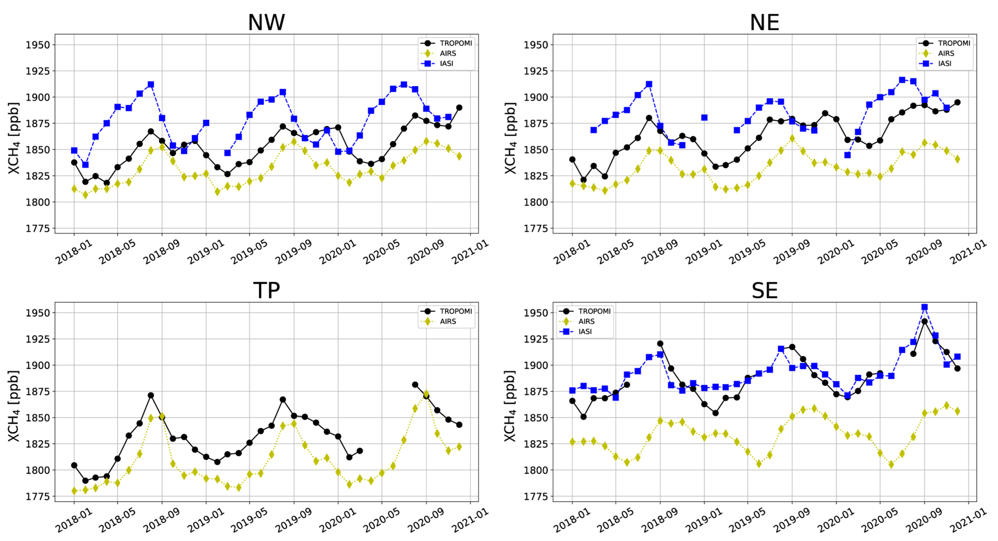
3.3. Temporal Variation of the Atmospheric CH₄ in China

In this section, we derive the XCH₄ seasonal means in China (Figure 9(e1,e2)). All the four satellite measurements show high CH₄ concentrations in summer and autumn, and low in winter and spring.

The XCH₄ values obtained from the GOSAT have very sparse coverage; it is hard to see its phase pattern (Figure 9(a1–a4)). The spatial pattern of the TROPOMI XCH₄ remains consistent throughout the four seasons (Figure 9(b1–b4)).

In contrast, the XCH₄ values from the AIRS vary significantly with time. Notably, in winter, the AIRS XCH₄ is high in the south and low in the north (Figure 9(c1)), while, in summer, the AIRS XCH₄ is low in the south and high in the north (Figure 9(c3)). Moreover, relatively high AIRS XCH₄ measurements are found in Inner Mongolia, especially during winter and spring, which has been discussed in Section 3.1. Figure 9(d1–d4,e1,e2) show that the IASI CH₄ measurements are systematically higher than the other three satellites, especially during spring and summer seasons.

Figure 10 shows the monthly average XCH₄ in the four regions. To reduce the sampling error, we only took the monthly mean in regions with more than 100 individual bins. Due to the limited amount of the GOSAT data, it was filtered out. Note that there are also some missing months for the IASI measurements.

The TROPOMI measurements show that the seasonal variations of XCH₄ in the four regions are consistent, with a high XCH₄ value in summer. According to the previous study, the seasonal variation of CH₄ in China is dominated by wetland and rice paddies due to large rice production in summer [40]. In TP, the TROPOMI and AIRS measurements have a similar seasonal variation in terms of both amplitude and phase, where a maximum in the late summer and early autumn, and a minimum value in late winter and early spring are observed. The amplitudes of the seasonal variation derived from both satellites are about 90 ppb, indicating a similar variation in the near-surface and mid-to-upper troposphere in TP. In SE, the seasonal variations of CH₄ observed by the TROPOMI and IASI are similar, with a maximum in late summer and early autumn and a minimum in winter. However, the AIRS XCH₄ shows a different seasonal variation compared to the IASI and TROPOMI, with a minimum in May–July and a maximum in October–December. In NE and NW, the TROPOMI measurements have a bimodal peak (summer and autumn). The AIRS measurements generally have a consistent seasonal variation with the TROPOMI. However, the seasonal variation of CH₄ in NE and NW derived from the IASI measurements has a much larger amplitude, and the maximum peak derived from the IASI measurements occurs 1–3 months in advance compared to the other two satellites.

4. Conclusions

The study presents and discusses the spatiotemporal variations of CH₄ in China between 2018 and 2020 from four satellites. The GOSAT and TROPOMI CH₄ data are retrieved from the SWIR spectra, with a good sensitivity in the troposphere and stratosphere. The mean and standard deviation between the GOSAT and TROPOMI XCH₄ are −13.8 ± 18.3 ppb and a good correlation was found between them (R = 0.78). They both observe high concentrations in the east and south, and low concentrations in the west and north, which is consistent with the CH₄ anthropogenic emission inventory.

The AIRS and IASI use TIR spectra, mainly sensitive to the upper troposphere and lower stratosphere. The spatial distributions of their CH₄ products are relatively uniform compared to the TROPOMI. However, the correlation between them is relatively weak, especially in high-latitude regions. Using the CAMS model as an independent reference, we find that the AIRS measurements better present the CH₄ variation in the upper troposphere and lower stratosphere compared to the IASI measurements.

As expected, large differences between the TROPOMI (SWIR) and AIRS (TIR) XCH₄ measurements are observed in China. We find that the differences between the two XCH₄ datasets are highly related to the CH₄ emissions. For example, in southeastern China where there are high CH₄ emissions, the difference between the TROPOMI and AIRS is up to 80 ppb. The reason is that the a priori profile for the AIRS CH₄ in the lower troposphere is considerably underestimated in these areas.

In terms of the temporal variation, the four satellites all show that the XCH₄ in China is high in summer and autumn, and low in winter and spring. It is noteworthy that the AIRS XCH₄ shows extremely high values in winter and spring in NW, which may be due to the low emissivity in this area. IASI has a good agreement with TROPOMI in SE, while it deviates from TROPOMI and AIRS in NW and NE.

Overall, this study provides insight into the spatiotemporal variations of CH₄ in China, and compares the CH₄ datasets from four widely used satellites. Differences do exist in terms of both spatial and temporal distributions of CH₄, and cautions must be taken when using these satellite products in China.

References

1. Cao, Y.; Li, X.; Yan, H.; Kuang, S. China’s Efforts to Peak Carbon Emissions: Targets and Practice. Chin. J. Urban Environ. Stud. 2021, 9, 2150004. [Google Scholar] [CrossRef]
2. IPCC. Climate Change 2013: The Physical Science Basis. Contribution of Working Group I to the Fifth Assessment Report of the Intergovernmental Panel on Climate Change; IPCC: Geneva, Switzerland, 2013. [Google Scholar]
3. Ehhalt, D.H.; Schmidt, U. Sources and Sinks of Atmospheric Methane. Pure Appl. Geophys. 1978, 116, 452–464. [Google Scholar] [CrossRef]
4. Hogan, K.B.; Hoffman, J.S.; Thompson, A.M. Methane on the Greenhouse Agenda. Nature 1991, 354, 181–182. [Google Scholar] [CrossRef]
5. Stocker, T.F.; Qin, D.; Plattner, G.K.; Tignor, M.M.B.; Allen, S.K.; Boschung, J.; Nauels, A.; Xia, Y.; Bex, V.; Midgley, P.M. Working Group I Contribution to the Fifth Assessment Report of the Intergovernmental Panel on Climate Change 14; IPCC: Geneva, Switzerland, 2015. [Google Scholar]
6. Solarin, S.A.; Gil-Alana, L.A. Persistence of Methane Emission in OECD Countries for 1750–2014: A Fractional Integration Approach. Environ. Model. Assess. 2021, 26, 497–509. [Google Scholar] [CrossRef]
7. Zhang, J.; Han, G.; Mao, H.; Pei, Z.; Ma, X.; Jia, W.; Gong, W. The Spatial and Temporal Distribution Patterns of XCH4 in China: New Observations from TROPOMI. Atmosphere 2022, 13, 177. [Google Scholar] [CrossRef]
8. Jacob, D.J.; Turner, A.J.; Maasakkers, J.D.; Sheng, J.; Sun, K.; Liu, X.; Chance, K.; Aben, I.; McKeever, J.; Frankenberg, C. Satellite Observations of Atmospheric Methane and Their Value for Quantifying Methane Emissions. Atmos. Chem. Phys. 2016, 16, 14371–14396. [Google Scholar] [CrossRef]
9. Maasakkers, J.D.; Varon, D.J.; Elfarsdóttir, A.; McKeever, J.; Jervis, D.; Mahapatra, G.; Pandey, S.; Lorente, A.; Borsdorff, T.; Foorthuis, L.R.; et al. Using Satellites to Uncover Large Methane Emissions from Landfills. Sci. Adv. 2022, 8, eabn9683. [Google Scholar] [CrossRef]
10. Qin, X.; Lei, L.; He, Z.; Zeng, Z.-C.; Kawasaki, M.; Ohashi, M.; Matsumi, Y. Preliminary Assessment of Methane Concentration Variation Observed by GOSAT in China. Adv. Meteorol. 2015, 2015, 125059. [Google Scholar] [CrossRef]
11. Lei, L.; Liu, Q.; Zhang, L.; Liu, L.; Zhang, B. A Preliminary Investigation of CO2 and CH4 Concentration Variations with the Land Use in Northern China by GOSAT. In Proceedings of the 2010 IEEE International Geoscience and Remote Sensing Symposium, Honolulu, HI, USA, 25–30 July 2010; pp. 1141–1144. [Google Scholar] [CrossRef]
12. Wang, H.; Li, J.; Zhang, Y.; Li, S.; Zhang, L.; Chen, L. Spatial and temporal distribution of near-surface methane concentration over China based on AIRS observations. J. Remote Sens. 2015, 19, 827–835. [Google Scholar] [CrossRef]
13. Zhou, J.; Guan, L. Characteristics of Spatial and Temporal Distributions of Methane over the Tibetan Plateau and Mechanism Analysis for High Methane Concentration in Summer. Clim. Environ. Res. 2017, 22, 315–321. [Google Scholar] [CrossRef]
14. Feng, D.; Gao, X.; Yang, L.; Hui, X.; Zhou, Y. A spatial-temporal distribution characteristics of the atmospheric methane in troposphere on Qinghai-Tibetan plateau using ARIS data. Chin. Environ. Sci. 2017, 37, 2822–2830. [Google Scholar] [CrossRef]
15. Zhang, X.; Bai, W.; Zhang, P.; Wang, W. Spatiotemporal Variations in Mid-Upper Tropospheric Methane over China from Satellite Observations. Chin. Sci. Bull. 2011, 56, 3321. [Google Scholar] [CrossRef]
16. Xu, Y.; Wang, J.; Sun, J.; Xu, Y.; Harris, W. Spatial and Temporal Variations of Lower Tropospheric Methane During 2010–2011 in China. IEEE J. Stars 2012, 5, 1464–1473. [Google Scholar] [CrossRef]
17. Wu, X.; Zhang, X.; Chuai, X.; Huang, X.; Wang, Z. Long-Term Trends of Atmospheric CH4 Concentration across China from 2002 to 2016. Remote Sens. 2019, 11, 538. [Google Scholar] [CrossRef]
18. Kuze, A.; Suto, H.; Nakajima, M.; Hamazaki, T. Thermal and near Infrared Sensor for Carbon Observation Fourier-Transform Spectrometer on the Greenhouse Gases Observing Satellite for Greenhouse Gases Monitoring. Appl. Opt. 2009, 48, 6716. [Google Scholar] [CrossRef]
19. Lorente, A.; Borsdorff, T.; Butz, A.; Hasekamp, O.; aan de Brugh, J.; Schneider, A.; Wu, L.; Hase, F.; Kivi, R.; Wunch, D.; et al. Methane Retrieved from TROPOMI: Improvement of the Data Product and Validation of the First 2 Years of Measurements. Atmos. Meas. Tech. 2021, 14, 665–684. [Google Scholar] [CrossRef]
20. Crevoisier, C.; Nobileau, D.; Fiore, A.M.; Armante, R.; Chédin, A.; Scott, N.A. Tropospheric Methane in the Tropics—First Year from IASI Hyperspectral Infrared Observations. Atmos. Chem. Phys. 2009, 9, 6337–6350. [Google Scholar] [CrossRef]
21. Xiong, X.; Barnet, C.; Maddy, E.; Sweeney, C.; Liu, X.; Zhou, L.; Goldberg, M. Characterization and Validation of Methane Products from the Atmospheric Infrared Sounder (AIRS). J. Geophys. Res. Biogeosci. 2008, 113, JG000500. [Google Scholar] [CrossRef]
22. Shi, C.; Hashimoto, M.; Shiomi, K.; Nakajima, T. Development of an Algorithm to Retrieve Aerosol Optical Properties Over Water Using an Artificial Neural Network Radiative Transfer Scheme: First Result From GOSAT-2/CAI-2. IEEE Trans. Geosci. Remote Sens. 2021, 59, 9861–9872. [Google Scholar] [CrossRef]
23. Zhou, M.; Dils, B.; Wang, P.; Detmers, R.; Yoshida, Y.; O’Dell, C.W.; Feist, D.G.; Velazco, V.A.; Schneider, M.; De Mazière, M. Validation of TANSO-FTS/GOSAT XCO2 and XCH4 Glint Mode Retrievals Using TCCON Data from near-Ocean Sites. Atmos. Meas. Tech. 2016, 9, 1415–1430. [Google Scholar] [CrossRef]
24. Imasu, R.; Matsunaga, T.; Nakajima, M.; Yoshida, Y.; Shiomi, K.; Morino, I.; Saitoh, N.; Niwa, Y.; Someya, Y.; Oishi, Y.; et al. Greenhouse Gases Observing SATellite 2 (GOSAT-2): Mission Overview. Prog. Earth Planet. Sci. 2023, 10, 33. [Google Scholar] [CrossRef]
25. Butz, A.; Hasekamp, O.P.; Frankenberg, C.; Vidot, J.; Aben, I. CH4 Retrievals from Space-Based Solar Backscatter Measurements: Performance Evaluation against Simulated Aerosol and Cirrus Loaded Scenes. J. Geophys. Res. 2010, 115, JD014514. [Google Scholar] [CrossRef]
26. Borsdorff, T.; Aan de Brugh, J.; Hu, H.; Aben, I.; Hasekamp, O.; Landgraf, J. Measuring Carbon Monoxide With TROPOMI: First Results and a Comparison With ECMWF-IFS Analysis Data. Geophys. Res. Lett. 2018, 45, 2826–2832. [Google Scholar] [CrossRef]
27. Crevoisier, C.; Nobileau, D.; Armante, R.; Crépeau, L.; Machida, T.; Sawa, Y.; Matsueda, H.; Schuck, T.; Thonat, T.; Pernin, J.; et al. The 2007–2011 Evolution of Tropical Methane in the Mid-Troposphere as Seen from Space by MetOp-A/IASI. Atmos. Chem. Phys. 2013, 13, 4279–4289. [Google Scholar] [CrossRef]
28. Qin, J.; Zhang, X.; Zhang, L.; Cheng, M.; Lu, X. Spatiotemporal Variations of XCH4 across China during 2003–2021 Based on Observations from Multiple Satellites. Atmosphere 2022, 13, 1362. [Google Scholar] [CrossRef]
29. Miller, S.M.; Wofsy, S.C.; Michalak, A.M.; Kort, E.A.; Andrews, A.E.; Biraud, S.C.; Dlugokencky, E.J.; Eluszkiewicz, J.; Fischer, M.L.; Janssens-Maenhout, G.; et al. Anthropogenic Emissions of Methane in the United States. Proc. Natl. Acad. Sci. USA 2013, 110, 20018–20022. [Google Scholar] [CrossRef]
30. Wang, F.; Maksyutov, S.; Janardanan, R.; Tsuruta, A.; Ito, A.; Morino, I.; Yoshida, Y.; Tohjima, Y.; Kaiser, J.W.; Lan, X.; et al. Atmospheric Observations Suggest Methane Emissions in North-Eastern China Growing with Natural Gas Use. Sci. Rep. 2022, 12, 18587. [Google Scholar] [CrossRef] [PubMed]
31. Koffi, E.N.; Bergamaschi, P. Evaluation of Copernicus Atmosphere Monitoring Service Methane Products; Joint Research Centre: Ispra, Italy, 2018. [Google Scholar]
32. Agusti-Panareda, A.; Barré, J.; Massart, S.; Inness, A.; Aben, I.; Ades, M.; Baier, B.C.; Balsamo, G.; Borsdorff, T.; Bousserez, N.; et al. Technical Note: The CAMS Greenhouse Gas Reanalysis from 2003 to 2020. Atmos. Chem. Phys. 2023, 23, 3829–3859. [Google Scholar] [CrossRef]
33. Sadavarte, P.; Pandey, S.; Maasakkers, J.D.; Lorente, A.; Borsdorff, T.; van der Gon, H.D.; Houweling, S.; Aben, I. Methane Emissions from Superemitting Coal Mines in Australia Quantified Using TROPOMI Satellite Observations. Environ. Sci. Technol. 2021, 55, 16573–16580. [Google Scholar] [CrossRef]
34. Plant, G.; Kort, E.A.; Murray, L.T.; Maasakkers, J.D.; Aben, I. Evaluating Urban Methane Emissions from Space Using TROPOMI Methane and Carbon Monoxide Observations. Remote Sens. Environ. 2022, 268, 112756. [Google Scholar] [CrossRef]
35. Olioso, A.; Sòria, G.; Sobrino, J.; Duchemin, B. Evidence of low land surface thermal infrared emissivity in the presence of dry vegetation. IEEE Geosci. Remote Sens. Lett. 2007, 4, 112–116. [Google Scholar] [CrossRef]
36. Qu, Z.; Jacob, D.J.; Shen, L.; Lu, X.; Zhang, Y.; Scarpelli, T.R.; Nesser, H.; Sulprizio, M.P.; Maasakkers, J.D.; Bloom, A.A.; et al. Global Distribution of Methane Emissions: A Comparative Inverse Analysis of Observations from the TROPOMI and GOSAT Satellite Instruments. Atmos. Chem. Phys. 2021, 21, 14159–14175. [Google Scholar] [CrossRef]
37. Misra, V.; DiNapoli, S. The Variability of the Southeast Asian Summer Monsoon: Variability of the Southeast Monsoon. Int. J. Climatol. 2014, 34, 893–901. [Google Scholar] [CrossRef]
38. Xiong, X.; Houweling, S.; Wei, J.; Maddy, E.; Sun, F.; Barnet, C. Methane Plume over South Asia during the Monsoon Season: Satellite Observation and Model Simulation. Atmos. Chem. Phys. 2009, 9, 783–794. [Google Scholar] [CrossRef]
39. Hu, H.; Hasekamp, O.; Butz, A.; Galli, A.; Landgraf, J.; Aan De Brugh, J.; Borsdorff, T.; Scheepmaker, R.; Aben, I. The Operational Methane Retrieval Algorithm for TROPOMI. Atmos. Meas. Tech. 2016, 9, 5423–5440. [Google Scholar] [CrossRef]
40. Zhang, G.; Xiao, X.; Dong, J.; Xin, F.; Zhang, Y.; Qin, Y.; Doughty, R.B.; Moore, B. Fingerprint of Rice Paddies in Spatial–Temporal Dynamics of Atmospheric Methane Concentration in Monsoon Asia. Nat. Commun. 2020, 11, 554. [Google Scholar] [CrossRef] [PubMed]
Figure 1. The volume of CH4 emissions recorded by EGDAR in four areas above China for the year 2018, namely north-eastern China (NE), south-eastern China (SE), north-western China (NW), and the Qinghai–Tibetan Plateau (TP).
Remotesensing 15 04499 g001
Figure 2. Typical vertical sensitivities as a function of pressure for satellites’ observations of CH4 in SWIR (GOSAT and TROPOMI) and TIR (IASI and AIRS).
Remotesensing 15 04499 g002
Figure 3. Annual average distribution of XCH4 in China from 2018 to 2020.
Remotesensing 15 04499 g003
Figure 4. The spatial distribution of AIRS XCH4 (a) and surface emissivity around 1300 cm−1 (b), the black triangles are bare soil surface types.
Remotesensing 15 04499 g004
Figure 5. Scatter plots of the GOSAT and TROPOMI XCH4 in the NE, SE, NW, and TP areas. The red dashed line is the linear fitting (y = ax + b) and the black solid line corresponds to the 1:1 line. R is the Pearson correlation coefficient. N is the number of co-located data.
Remotesensing 15 04499 g005
Figure 6. The scatter plots of the IASI XCH4 and AIRS (a1a4) and the CAMS (b1b4) average CH4 concentration between 100 and 300 hPa in China, NW, NE, and SE. The scatter plots of the CAMS average CH4 concentration between 100 and 300 hPa and the AIRS average CH4 concentration between 100 and 300 hPa (c1c4) in China, NW, NE, and SE. The red dashed line is the linear fitting (y = ax + b). R is the Pearson correlation coefficient. N is the number of co-located data.
Remotesensing 15 04499 g006
Figure 7. Scatter plots of the TROPOMI and AIRS XCH4 in the NW, NE, TP, and SE areas. The red dashed line is the linear fitting (y = ax + b). R is the Pearson correlation coefficient. N is the number of co-located data.
Remotesensing 15 04499 g007
Figure 8. The spatial distribution of the difference between the TROPOMI and AIRS XCH4 (a). The frequency histogram of the differences, together with the EDGAR CH4 emissions (b). The orange line represents the average CH4 emissions in each difference interval.
Remotesensing 15 04499 g008
Figure 9. Spatial distributions of the seasonal averages of XCH4 concentrations across China in the four seasons from GOSAT (2018–2019; (a1a4)), TROPOMI (2018–2020; (b1b4)), AIRS (2018–2020; (c1c4)), and IASI (2018–2020; (d1d4)), together with the monthly variations of XCH4 concentrations over China (e1,e2).
Remotesensing 15 04499 g009
Figure 10. Time series of CH4 monthly means in the four study areas.
Remotesensing 15 04499 g010