


Flood Extent and Volume Estimation Using Remote Sensing Data

 ,
,  , ,
, ,  ,
, 
Abstract
:1. Introduction
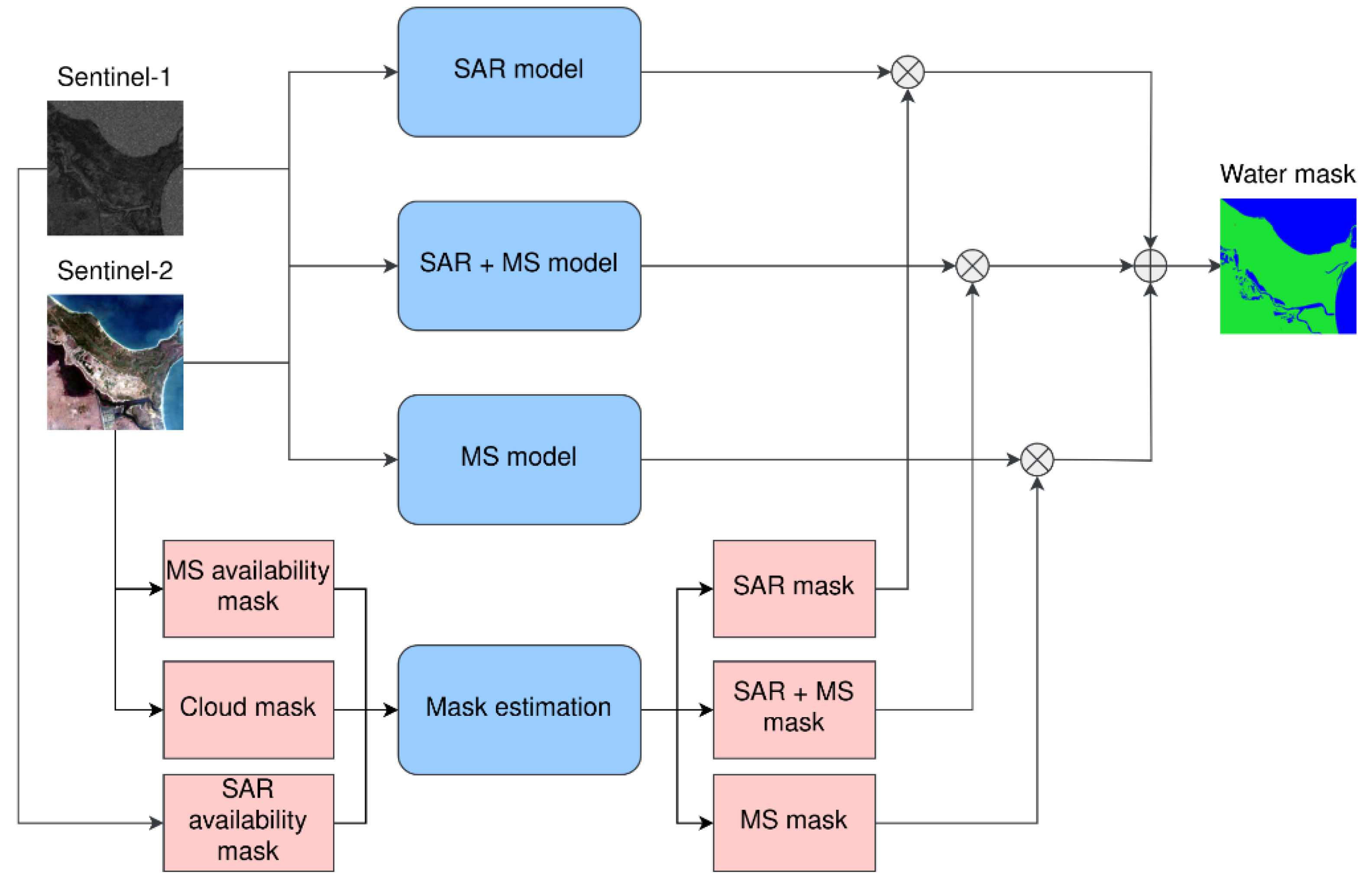
- We proposed a flood extension estimation pipeline based on Sentinel-1 and Sentinel-2 data that utilizes neural network technology;
- We took into account possible real-life limitations such as satellite data availability and cloud coverage during flood events;
- We explored different deep learning architectures and investigated feature spaces to optimize our approach;
- Additionally, we developed a method for flood volume estimation that utilizes both DEM and predicted flood extent.
2. Materials and Methods
2.1. Dataset
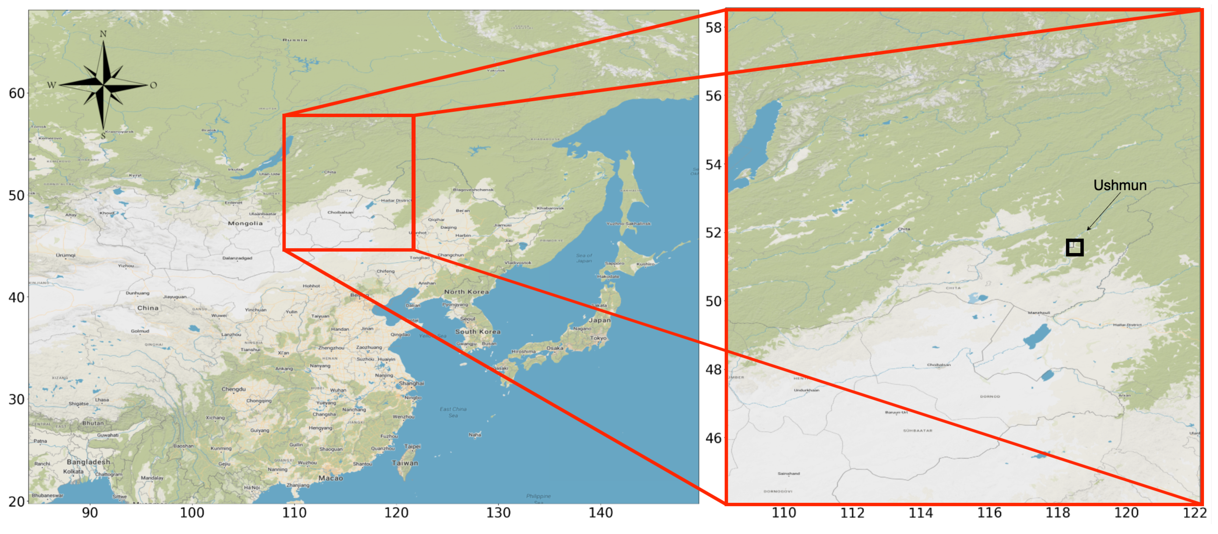
2.1.1. Data Description
2.1.2. Image Processing
- —Normalized Difference Water Index. It emphasizes water bodies and vegetation water content [29];
- —Modified Normalized Difference Water Index. It is similar to NDWI, but reduces sensitivity to dense vegetation, making it more effective for open water body detection [30];
- —Standardized Water-Level Index. It estimates soil moisture content by analyzing the difference between near-infrared and shortwave infrared reflectance [31];
- , —Automated Water Extraction Index. Both and are indices tailored for water body detection, with leveraging shortwave infrared data for enhanced accuracy and offering an alternative when shortwave data are lacking [32].
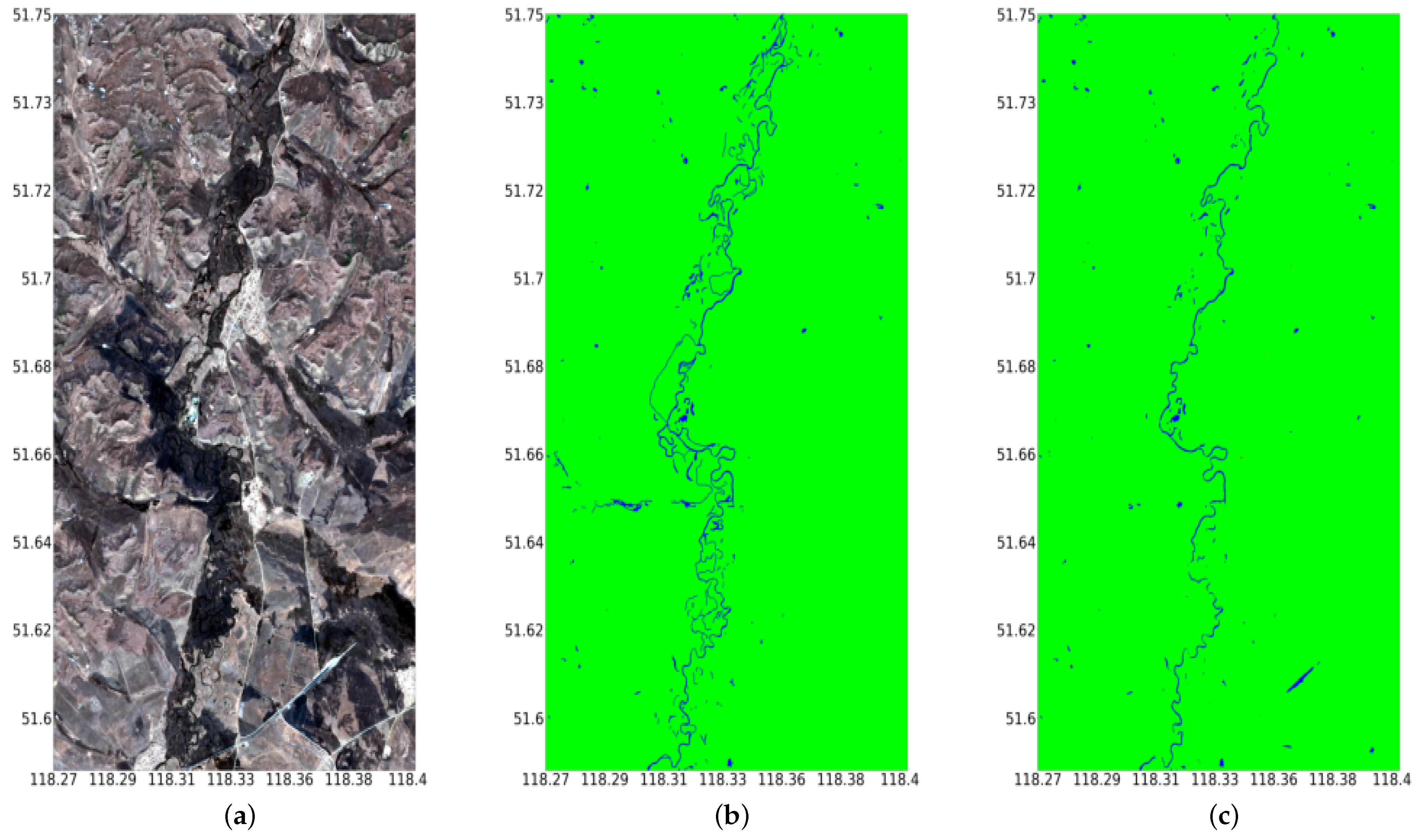
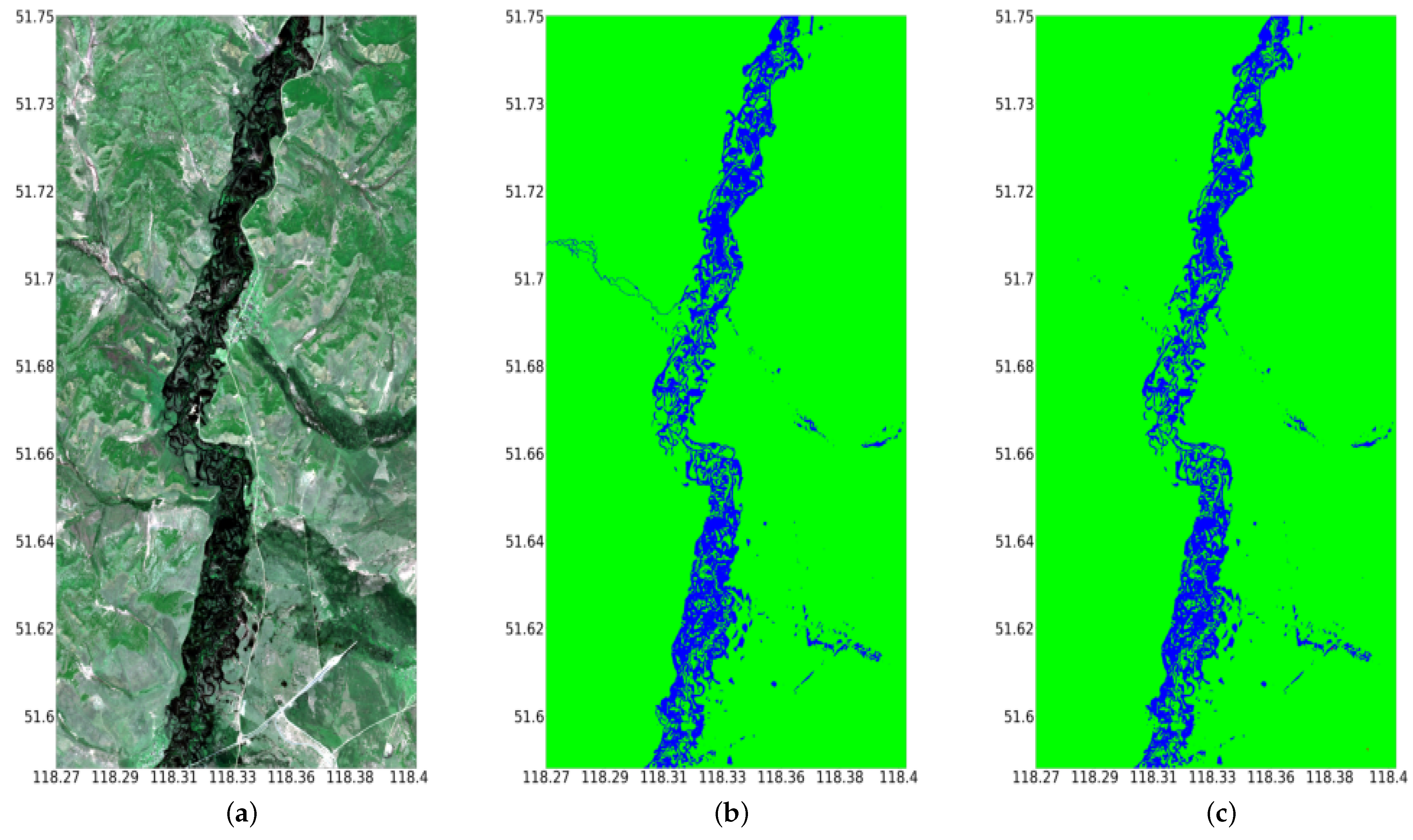
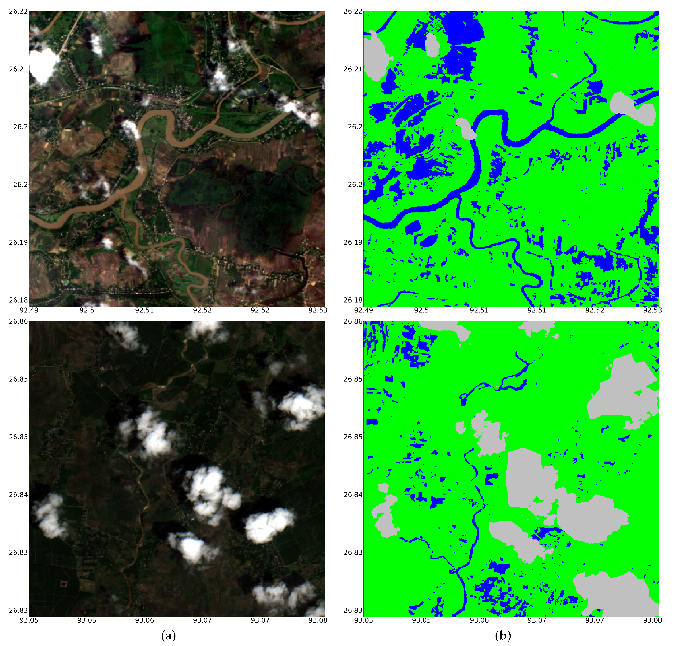
2.1.3. External Test Data
2.2. Methods
2.2.1. Flood Extent
2.2.2. Flood Volume
2.3. Evaluation Metrics
3. Results
3.1. Results on Sen1Floods11 Dataset
3.2. Results on External Data
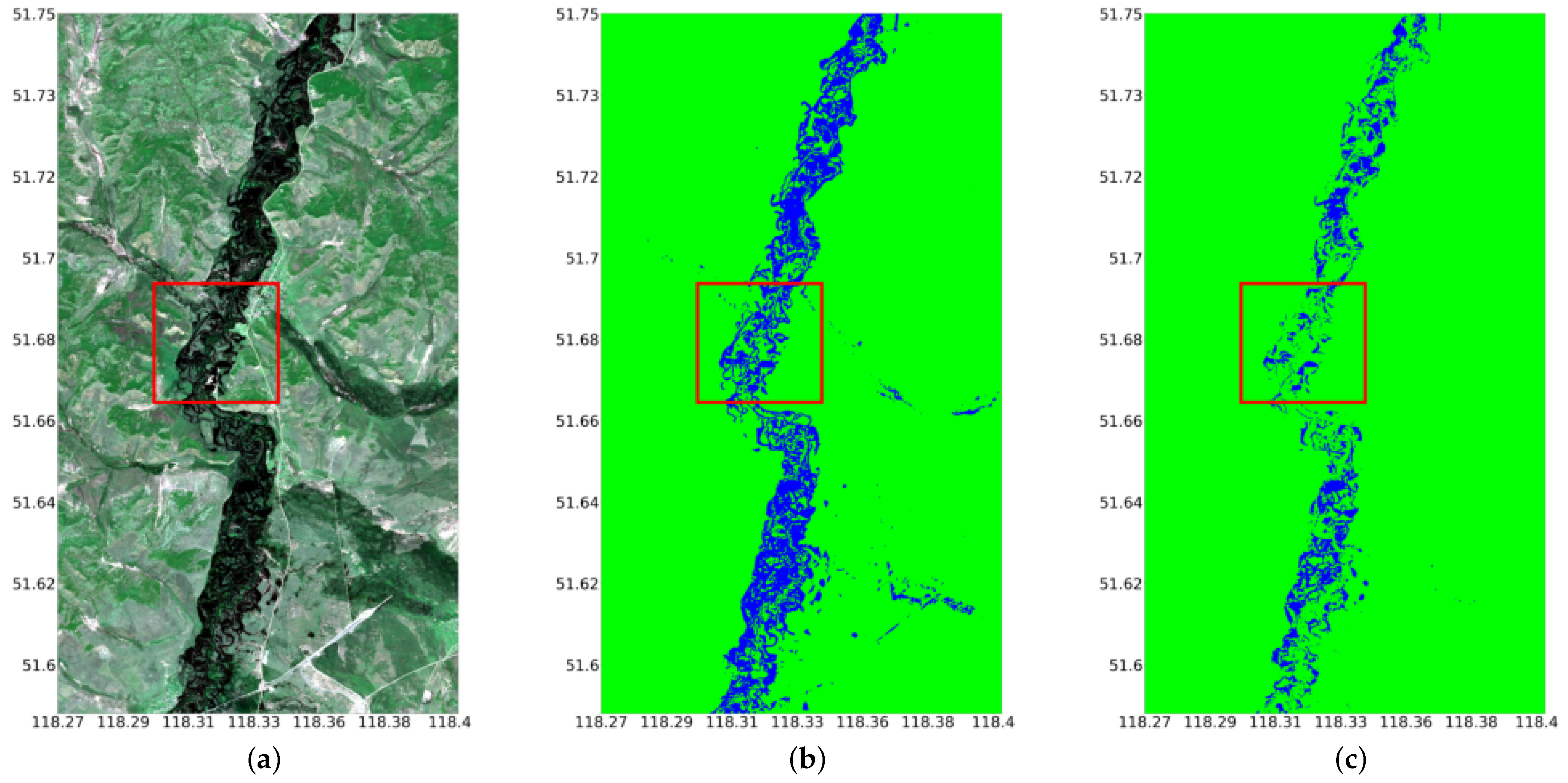
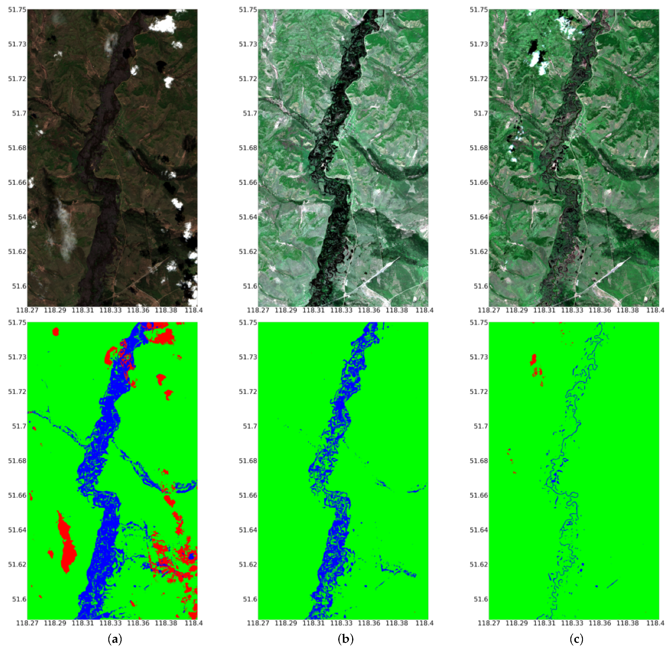
3.2.1. Flood Extent
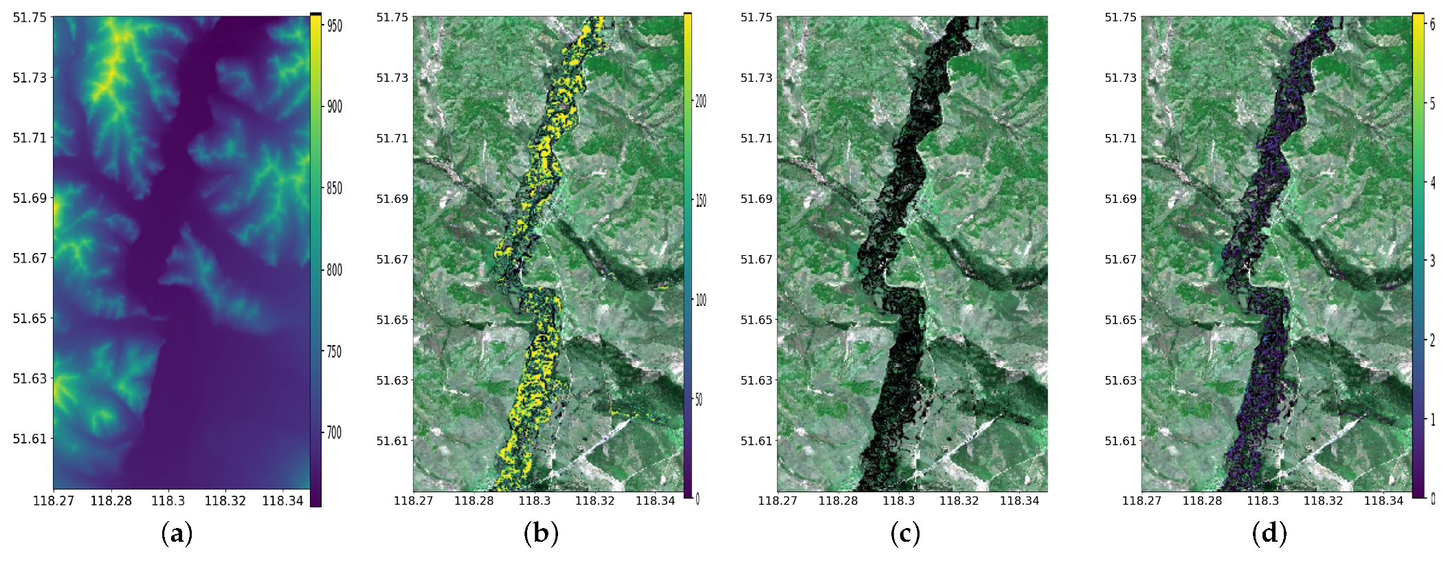
3.2.2. Flood Volume
4. Discussion
5. Conclusions
Author Contributions
Funding
Data Availability Statement
Conflicts of Interest
Abbreviations
| ALWS | Absolute level of the water surface |
| AWEI | Automated Water Extraction Index |
| BASNet | Boundary-Aware Salient Network |
| BF | Beyond flood |
| DEM | Digital Elevation Model |
| DF | During flood |
| IoU | Intersection over Union |
| MNDWI | Modified Normalized Difference Water Index |
| MS | Multispectral |
| NDWI | Normalized Difference Water Index |
| NIR | Near-Infrared |
| OSM | OpenStreetMap |
| SAR | Synthetic Aperture Radar |
| SWI | Standardized Water-Level Index |
| SWIR | Short-Wave Infrared |
References
- Sharma, T.P.P.; Zhang, J.; Koju, U.A.; Zhang, S.; Bai, Y.; Suwal, M.K. Review of flood disaster studies in Nepal: A remote sensing perspective. Int. J. Disaster Risk Reduct. 2019, 34, 18–27. [Google Scholar] [CrossRef]
- Munawar, H.S.; Hammad, A.W.; Waller, S.T. Remote sensing methods for flood prediction: A review. Sensors 2022, 22, 960. [Google Scholar] [CrossRef]
- Illarionova, S.; Shadrin, D.; Tregubova, P.; Ignatiev, V.; Efimov, A.; Oseledets, I.; Burnaev, E. A Survey of Computer Vision Techniques for Forest Characterization and Carbon Monitoring Tasks. Remote Sens. 2022, 14, 5861. [Google Scholar] [CrossRef]
- Illarionova, S.; Shadrin, D.; Shukhratov, I.; Evteeva, K.; Popandopulo, G.; Sotiriadi, N.; Oseledets, I.; Burnaev, E. Benchmark for Building Segmentation on Up-Scaled Sentinel-2 Imagery. Remote Sens. 2023, 15, 2347. [Google Scholar] [CrossRef]
- Chawla, I.; Karthikeyan, L.; Mishra, A.K. A review of remote sensing applications for water security: Quantity, quality, and extremes. J. Hydrol. 2020, 585, 124826. [Google Scholar]
- Hernández, D.; Cecilia, J.M.; Cano, J.C.; Calafate, C.T. Flood detection using real-time image segmentation from unmanned aerial vehicles on edge-computing platform. Remote Sens. 2022, 14, 223. [Google Scholar] [CrossRef]
- Feng, Q.; Liu, J.; Gong, J. Urban flood mapping based on unmanned aerial vehicle remote sensing and random forest classifier—A case of Yuyao, China. Water 2015, 7, 1437–1455. [Google Scholar] [CrossRef]
- Hashemi-Beni, L.; Gebrehiwot, A.A. Flood extent mapping: An integrated method using deep learning and region growing using UAV optical data. IEEE J. Sel. Top. Appl. Earth Obs. Remote Sens. 2021, 14, 2127–2135. [Google Scholar] [CrossRef]
- Chien, S.; Mclaren, D.; Doubleday, J.; Tran, D.; Tanpipat, V.; Chitradon, R. Using taskable remote sensing in a sensor web for Thailand flood monitoring. J. Aerosp. Inf. Syst. 2019, 16, 107–119. [Google Scholar] [CrossRef]
- Lin, L.; Di, L.; Tang, J.; Yu, E.; Zhang, C.; Rahman, M.S.; Shrestha, R.; Kang, L. Improvement and validation of NASA/MODIS NRT global flood mapping. Remote Sens. 2019, 11, 205. [Google Scholar] [CrossRef]
- Moortgat, J.; Li, Z.; Durand, M.; Howat, I.; Yadav, B.; Dai, C. Deep learning models for river classification at sub-meter resolutions from multispectral and panchromatic commercial satellite imagery. Remote Sens. Environ. 2022, 282, 113279. [Google Scholar] [CrossRef]
- Zhang, L.; Xia, J. Flood detection using multiple chinese satellite datasets during 2020 china summer floods. Remote Sens. 2022, 14, 51. [Google Scholar] [CrossRef]
- Islam, M.M.; Ahamed, T. Development of a near-infrared band derived water indices algorithm for rapid flash flood inundation mapping from sentinel-2 remote sensing datasets. Asia-Pac. J. Reg. Sci. 2023, 7, 615–640. [Google Scholar] [CrossRef]
- Sivanpillai, R.; Jacobs, K.M.; Mattilio, C.M.; Piskorski, E.V. Rapid flood inundation mapping by differencing water indices from pre-and post-flood Landsat images. Front. Earth Sci. 2021, 15, 1–11. [Google Scholar] [CrossRef]
- Jones, J.W. Improved automated detection of subpixel-scale inundation—Revised dynamic surface water extent (DSWE) partial surface water tests. Remote Sens. 2019, 11, 374. [Google Scholar] [CrossRef]
- Jet Propulsion Laboratory. Observational Products for End-Users from Remote Sensing Analysis (OPERA). 2023. Available online: https://www.jpl.nasa.gov/go/opera (accessed on 20 June 2023).
- Chen, Z.; Zhao, S. Automatic monitoring of surface water dynamics using Sentinel-1 and Sentinel-2 data with Google Earth Engine. Int. J. Appl. Earth Obs. Geoinf. 2022, 113, 103010. [Google Scholar] [CrossRef]
- Dong, Z.; Wang, G.; Amankwah, S.O.Y.; Wei, X.; Hu, Y.; Feng, A. Monitoring the summer flooding in the Poyang Lake area of China in 2020 based on Sentinel-1 data and multiple convolutional neural networks. Int. J. Appl. Earth Obs. Geoinf. 2021, 102, 102400. [Google Scholar] [CrossRef]
- Bonafilia, D.; Tellman, B.; Anderson, T.; Issenberg, E. Sen1Floods11: A georeferenced dataset to train and test deep learning flood algorithms for sentinel-1. In Proceedings of the IEEE/CVF Conference on Computer Vision and Pattern Recognition Workshops, Seattle, WA, USA, 14–19 June 2020; pp. 210–211. [Google Scholar]
- Bai, Y.; Wu, W.; Yang, Z.; Yu, J.; Zhao, B.; Liu, X.; Yang, H.; Mas, E.; Koshimura, S. Enhancement of detecting permanent water and temporary water in flood disasters by fusing sentinel-1 and sentinel-2 imagery using deep learning algorithms: Demonstration of sen1floods11 benchmark datasets. Remote Sens. 2021, 13, 2220. [Google Scholar] [CrossRef]
- Qin, X.; Zhang, Z.; Huang, C.; Gao, C.; Dehghan, M.; Jagersand, M. Basnet: Boundary-aware salient object detection. In Proceedings of the IEEE/CVF Conference on Computer Vision and Pattern Recognition, Long Beach, CA, USA, 15–20 June 2019; pp. 7479–7489. [Google Scholar]
- Rudner, T.G.; Rußwurm, M.; Fil, J.; Pelich, R.; Bischke, B.; Kopačková, V.; Biliński, P. Multi3net: Segmenting flooded buildings via fusion of multiresolution, multisensor, and multitemporal satellite imagery. In Proceedings of the AAAI Conference on Artificial Intelligence, Honolulu, HI, USA, 27 January–1 February 2019; Volume 33, pp. 702–709. [Google Scholar]
- Quinn, N.; Bates, P.D.; Neal, J.; Smith, A.; Wing, O.; Sampson, C.; Smith, J.; Heffernan, J. The spatial dependence of flood hazard and risk in the United States. Water Resour. Res. 2019, 55, 1890–1911. [Google Scholar] [CrossRef]
- Rakwatin, P.; Sansena, T.; Marjang, N.; Rungsipanich, A. Using multi-temporal remote-sensing data to estimate 2011 flood area and volume over Chao Phraya River basin, Thailand. Remote Sens. Lett. 2013, 4, 243–250. [Google Scholar] [CrossRef]
- Cohen, S.; Raney, A.; Munasinghe, D.; Loftis, J.D.; Molthan, A.; Bell, J.; Rogers, L.; Galantowicz, J.; Brakenridge, G.R.; Kettner, A.J.; et al. The Floodwater Depth Estimation Tool (FwDET v2. 0) for improved remote sensing analysis of coastal flooding. Nat. Hazards Earth Syst. Sci. 2019, 19, 2053–2065. [Google Scholar] [CrossRef]
- Cohen, S.; Brakenridge, G.R.; Kettner, A.; Bates, B.; Nelson, J.; McDonald, R.; Huang, Y.F.; Munasinghe, D.; Zhang, J. Estimating floodwater depths from flood inundation maps and topography. JAWRA J. Am. Water Resour. Assoc. 2018, 54, 847–858. [Google Scholar] [CrossRef]
- Budiman, J.; Bahrawi, J.; Hidayatulloh, A.; Almazroui, M.; Elhag, M. Volumetric quantification of flash flood using microwave data on a watershed scale in arid environments, Saudi Arabia. Sustainability 2021, 13, 4115. [Google Scholar] [CrossRef]
- Sinergise Ltd. Sentinel Hub: Cloud-Based Processing and Analysis of Satellite Data. Available online: https://www.sentinel-hub.com/ (accessed on 20 June 2023).
- McFeeters, S.K. The use of the Normalized Difference Water Index (NDWI) in the delineation of open water features. Int. J. Remote Sens. 1996, 17, 1425–1432. [Google Scholar] [CrossRef]
- Xu, H. Modification of normalised difference water index (NDWI) to enhance open water features in remotely sensed imagery. Int. J. Remote Sens. 2006, 27, 3025–3033. [Google Scholar] [CrossRef]
- Bagheri, H.; Moradi, M.; Sarikhani, M.R.; Tazeh, M. Soil water index determination using Landsat 8 OLI and TIRS sensor data. J. Appl. Remote Sens. 2015, 9, 096075. [Google Scholar]
- Fei, T.; Wang, C.; Li, X.; Zhou, Y.; Zhang, Z. Automatic Water Extraction Index (AWEI) for inland water body extraction with Landsat 8 OLI imagery. ISPRS J. Photogramm. Remote Sens. 2019, 147, 98–112. [Google Scholar]
- Main-Knorn, M.; Pflug, B.; Louis, J.; Debaecker, V.; Müller-Wilm, U.; Gascon, F. Sen2Cor for sentinel-2. In Proceedings of the Image and Signal Processing for Remote Sensing (XXIII SPIE), Warsaw, Poland, 11–13 September 2017; Volume 10427, pp. 37–48. [Google Scholar]
- Ronneberger, O.; Fischer, P.; Brox, T. U-net: Convolutional networks for biomedical image segmentation. In Proceedings of the International Conference on Medical Image Computing and Computer-Assisted Intervention, Munich, Germany, 5–9 October 2015; pp. 234–241. [Google Scholar]
- Fan, T.; Wang, G.; Li, Y.; Wang, H. MA-Net: A Multi-Scale Attention Network for Liver and Tumor Segmentation. IEEE Access 2020, 8, 179656–179665. [Google Scholar] [CrossRef]
- Chen, L.C.; Papandreou, G.; Schroff, F.; Adam, H. Rethinking atrous convolution for semantic image segmentation. arXiv 2017, arXiv:1706.05587. [Google Scholar]
- Illarionova, S.; Shadrin, D.; Ignatiev, V.; Shayakhmetov, S.; Trekin, A.; Oseledets, I. Estimation of the Canopy Height Model From Multispectral Satellite Imagery with Convolutional Neural Networks. IEEE Access 2022, 10, 34116–34132. [Google Scholar] [CrossRef]
- Sharma, S. Semantic Segmentation for Urban-Scene Images. arXiv 2021, arXiv:2110.13813. [Google Scholar]
- Deng, J.; Dong, W.; Socher, R.; Li, L.J.; Li, K.; Fei-Fei, L. ImageNet: A large-scale hierarchical image database. In Proceedings of the IEEE Conference on Computer Vision and Pattern Recognition, Miami, FL, USA, 20–25 June 2009. [Google Scholar]
- Sandler, M.; Howard, A.; Zhu, M.; Zhmoginov, A.; Chen, L.C. MobileNetV2: Inverted residuals and linear bottlenecks. In Proceedings of the Conference on Computer Vision and Pattern Recognition, Salt Lake City, UT, USA, 18–22 June 2018. [Google Scholar]
- He, K.; Zhang, X.; Ren, S.; Sun, J. Deep residual learning for image recognition. In Proceedings of the IEEE Conference on Computer Vision and Pattern Recognition, Las Vegas, NV, USA, 27–30 June 2016. [Google Scholar]
- Smith, L.N. Cyclical Learning Rates for Training Neural Networks. arXiv 2017, arXiv:1506.01186. [Google Scholar]
- Lin, T.Y.; Goyal, P.; Girshick, R.; He, K.; Dollár, P. Focal loss for dense object detection. In Proceedings of the IEEE International Conference on Computer Vision, Venice, Italy, 22–29 October 2017. [Google Scholar]
- Zhu, W.; Huang, Y.; Zeng, L.; Chen, X.; Liu, Y.; Qian, Z.; Du, N.; Fan, W.; Xie, X. AnatomyNet: Deep learning for fast and fully automated whole-volume segmentation of head and neck anatomy. Med. Phys. 2019, 46, 576–589. [Google Scholar] [CrossRef]
- Gao, Y.; Gella, G.W.; Liu, N. Assessing the Influences of Band Selection and Pretrained Weights on Semantic-Segmentation-Based Refugee Dwelling Extraction from Satellite Imagery. AGILE GISci. Ser. 2022, 3, 36. [Google Scholar] [CrossRef]
- Zhang, T.X.; Su, J.Y.; Liu, C.J.; Chen, W.H. Potential bands of sentinel-2A satellite for classification problems in precision agriculture. Int. J. Autom. Comput. 2019, 16, 16–26. [Google Scholar] [CrossRef]
- Pekel, J.F.; Cottam, A.; Gorelick, N.; Belward, A.S. High-resolution mapping of global surface water and its long-term changes. Nature 2016, 540, 418–422. [Google Scholar] [CrossRef]
- OpenStreetMap Contributors. 2017. Available online: https://www.openstreetmap.org (accessed on 20 May 2023).
- Illarionova, S.; Shadrin, D.; Ignatiev, V.; Shayakhmetov, S.; Trekin, A.; Oseledets, I. Augmentation-Based Methodology for Enhancement of Trees Map Detalization on a Large Scale. Remote Sens. 2022, 14, 2281. [Google Scholar] [CrossRef]
- Helleis, M.; Wieland, M.; Krullikowski, C.; Martinis, S.; Plank, S. Sentinel-1-Based Water and Flood Mapping: Benchmarking Convolutional Neural Networks Against an Operational Rule-Based Processing Chain. IEEE J. Sel. Top. Appl. Earth Obs. Remote Sens. 2022, 15, 2023–2036. [Google Scholar] [CrossRef]
- Mateo-Garcia, G.; Veitch-Michaelis, J.; Smith, L.; Oprea, S.V.; Schumann, G.; Gal, Y.; Baydin, A.G.; Backes, D. Towards global flood mapping onboard low cost satellites with machine learning. Sci. Rep. 2021, 11, 7249. [Google Scholar] [CrossRef]
- Romero, A.; Gatta, C.; Camps-Valls, G. Unsupervised deep feature extraction for remote sensing image classification. IEEE Trans. Geosci. Remote Sens. 2015, 54, 1349–1362. [Google Scholar] [CrossRef]
- Nesteruk, S.; Agafonova, J.; Pavlov, I.; Gerasimov, M.; Latyshev, N.; Dimitrov, D.; Kuznetsov, A.; Kadurin, A.; Plechov, P. MineralImage5k: A benchmark for zero-shot raw mineral visual recognition and description. Comput. Geosci. 2023, 178, 105414. [Google Scholar] [CrossRef]
- Yamazaki, D.; Ikeshima, D.; Tawatari, R.; Yamaguchi, T.; O’Loughlin, F.; Neal, J.C.; Sampson, C.C.; Kanae, S.; Bates, P.D. A high-accuracy map of global terrain elevations. Geophys. Res. Lett. 2017, 44, 5844–5853. [Google Scholar] [CrossRef]
- Nguyen, T.H.D.; Nguyen, T.C.; Nguyen, T.N.T.; Doan, T.N. Flood inundation mapping using Sentinel-1A in An Giang province in 2019. Vietnam. J. Sci. Technol. Eng. 2020, 62, 36–42. [Google Scholar] [CrossRef]
- Lincoln, T. Flood of data. Nature 2007, 447, 393. [Google Scholar] [CrossRef]
- Yang, T.; Sun, F.; Gentine, P.; Liu, W.; Wang, H.; Yin, J.; Du, M.; Liu, C. Evaluation and machine learning improvement of global hydrological model-based flood simulations. Environ. Res. Lett. 2019, 14, 114027. [Google Scholar] [CrossRef]
- Illarionova, S.; Nesteruk, S.; Shadrin, D.; Ignatiev, V.; Pukalchik, M.; Oseledets, I. Object-based augmentation for building semantic segmentation: Ventura and santa rosa case study. In Proceedings of the IEEE/CVF International Conference on Computer Vision, Montreal, BC, Canada, 10–17 October 2021; pp. 1659–1668. [Google Scholar]
- Mirpulatov, I.; Illarionova, S.; Shadrin, D.; Burnaev, E. Pseudo-Labeling Approach for Land Cover Classification through Remote Sensing Observations with Noisy Labels. IEEE Access 2023, 11, 82570–82583. [Google Scholar] [CrossRef]
- Pai, M.M.; Mehrotra, V.; Verma, U.; Pai, R.M. Improved semantic segmentation of water bodies and land in SAR images using generative adversarial networks. Int. J. Semant. Comput. 2020, 14, 55–69. [Google Scholar] [CrossRef]
- Nesteruk, S.; Illarionova, S.; Zherebzov, I.; Traweek, C.; Mikhailova, N.; Somov, A.; Oseledets, I. PseudoAugment: Enabling Smart Checkout Adoption for New Classes Without Human Annotation. IEEE Access 2023, 11, 76869–76882. [Google Scholar] [CrossRef]
- Jozdani, S.; Chen, D.; Pouliot, D.; Johnson, B.A. A review and meta-analysis of generative adversarial networks and their applications in remote sensing. Int. J. Appl. Earth Obs. Geoinf. 2022, 108, 102734. [Google Scholar] [CrossRef]
- Illarionova, S.; Shadrin, D.; Trekin, A.; Ignatiev, V.; Oseledets, I. Generation of the nir spectral band for satellite images with convolutional neural networks. Sensors 2021, 21, 5646. [Google Scholar] [CrossRef]
- Zacharov, I.; Arslanov, R.; Gunin, M.; Stefonishin, D.; Bykov, A.; Pavlov, S.; Panarin, O.; Maliutin, A.; Rykovanov, S.; Fedorov, M. “Zhores”—Petaflops supercomputer for data-driven modeling, machine learning and artificial intelligence installed in Skolkovo Institute of Science and Technology. Open Eng. 2019, 9, 512–520. [Google Scholar] [CrossRef]


| Area | Number of Images | |
|---|---|---|
| Train area | 6553.6 km2 | 250 images |
| Test area | 2175.8 km2 | 83 images |
| Validation area | 2175.8 km2 | 83 images |
| Date | Manual Markup | Position Relative to Flooding |
|---|---|---|
| 22 April 2021 | Yes | Beyond Flood |
| 4 June 2021 | No | During Flood |
| 6 June 2021 | Yes | During Flood |
| 11 June 2021 | No | Beyond Flood |
| Features Combination | MobileNetV2 | ResNet18 | ||
|---|---|---|---|---|
| F1-Score | IoU | F1-Score | IoU | |
| SAR | 0.777 | 0.636 | 0.781 | 0.641 |
| SAR + NDWI | 0.874 | 0.776 | 0.887 | 0.797 |
| SAR + MNDWI | 0.893 | 0.807 | 0.893 | 0.807 |
| SAR + SWI | 0.872 | 0.772 | 0.867 | 0.765 |
| SAR + | 0.85 | 0.74 | 0.857 | 0.75 |
| SAR + | 0.882 | 0.788 | 0.878 | 0.783 |
| MS | 0.917 | 0.847 | 0.913 | 0.84 |
| MS + SAR | 0.917 | 0.845 | 0.914 | 0.842 |
| SAR + All indices | 0.898 | 0.814 | 0.893 | 0.807 |
| MS + All indices | 0.903 | 0.824 | 0.895 | 0.809 |
| MS + SAR + All indices | 0.901 | 0.817 | 0.902 | 0.821 |
| Features Combination | MobileNetV2 | ResNet18 | ||
|---|---|---|---|---|
| F1-Score | IoU | F1-Score | IoU | |
| SAR | 0.792 | 0.655 | 0.792 | 0.655 |
| SAR + NDWI | 0.882 | 0.79 | 0.89 | 0.802 |
| SAR + MNDWI | 0.893 | 0.807 | 0.896 | 0.811 |
| SAR + SWI | 0.87 | 0.77 | 0.873 | 0.774 |
| SAR + | 0.856 | 0.748 | 0.851 | 0.741 |
| SAR + | 0.88 | 0.785 | 0.881 | 0.786 |
| MS | 0.915 | 0.843 | 0.909 | 0.833 |
| MS + SAR | 0.92 | 0.851 | 0.915 | 0.843 |
| SAR + All indices | 0.903 | 0.823 | 0.895 | 0.809 |
| MS + All indices | 0.896 | 0.811 | 0.897 | 0.813 |
| MS + SAR + All indices | 0.899 | 0.816 | 0.901 | 0.819 |
| Features Combination | MobileNetV2 | ResNet18 | ||
|---|---|---|---|---|
| F1-Score | IoU | F1-Score | IoU | |
| SAR | 0.781 | 0.641 | 0.793 | 0.657 |
| SAR + NDWI | 0.848 | 0.736 | 0.86 | 0.753 |
| SAR + MNDWI | 0.874 | 0.776 | 0.874 | 0.776 |
| SAR + SWI | 0.853 | 0.744 | 0.843 | 0.728 |
| SAR + | 0.838 | 0.722 | 0.832 | 0.711 |
| SAR + | 0.86 | 0.755 | 0.864 | 0.761 |
| MS | 0.887 | 0.797 | 0.886 | 0.796 |
| MS + SAR | 0.891 | 0.803 | 0.888 | 0.799 |
| SAR + All indices | 0.873 | 0.774 | 0.878 | 0.782 |
| MS + All indices | 0.879 | 0.784 | 0.88 | 0.786 |
| MS + SAR + All indices | 0.882 | 0.789 | 0.883 | 0.79 |
Disclaimer/Publisher’s Note: The statements, opinions and data contained in all publications are solely those of the individual author(s) and contributor(s) and not of MDPI and/or the editor(s). MDPI and/or the editor(s) disclaim responsibility for any injury to people or property resulting from any ideas, methods, instructions or products referred to in the content. |
© 2023 by the authors. Licensee MDPI, Basel, Switzerland. This article is an open access article distributed under the terms and conditions of the Creative Commons Attribution (CC BY) license (https://creativecommons.org/licenses/by/4.0/).
Share and Cite
Popandopulo, G.; Illarionova, S.; Shadrin, D.; Evteeva, K.; Sotiriadi, N.; Burnaev, E. Flood Extent and Volume Estimation Using Remote Sensing Data. Remote Sens. 2023, 15, 4463. https://doi.org/10.3390/rs15184463
Popandopulo G, Illarionova S, Shadrin D, Evteeva K, Sotiriadi N, Burnaev E. Flood Extent and Volume Estimation Using Remote Sensing Data. Remote Sensing. 2023; 15(18):4463. https://doi.org/10.3390/rs15184463
Chicago/Turabian StylePopandopulo, Georgii, Svetlana Illarionova, Dmitrii Shadrin, Ksenia Evteeva, Nazar Sotiriadi, and Evgeny Burnaev. 2023. "Flood Extent and Volume Estimation Using Remote Sensing Data" Remote Sensing 15, no. 18: 4463. https://doi.org/10.3390/rs15184463
APA StylePopandopulo, G., Illarionova, S., Shadrin, D., Evteeva, K., Sotiriadi, N., & Burnaev, E. (2023). Flood Extent and Volume Estimation Using Remote Sensing Data. Remote Sensing, 15(18), 4463. https://doi.org/10.3390/rs15184463