Empirical Correlation Weighting (ECW) Spatial Interpolation Method for Satellite Aerosol Optical Depth Products by MODIS AOD over Northern China in 2016

Abstract

Satellite aerosol products are pivotal in studies of regional air quality and global climate change. Compared with accurate in situ observations, satellite measurements provide valuable large-scale atmospheric information. However, limitations such as clouds and retrieval assumptions result in a significant number of missing values in satellite aerosol optical depth (AOD) products, which severely hampers the representativeness. To address this issue, spatial interpolation of the AOD data is necessary to improve data coverage. In this study, one year of AOD observation data from the MODIS C6.1 version was applied to analyze the spatiotemporal correlated characteristics. The statistical parameters were used as dynamic interpolation weights to develop a novel interpolation method called empirical correlation weighting (ECW) based on MODIS AOD over Northern China in 2016. The ECW interpolation results were obtained at a 0.05° resolution (~5 km). The results showed that the spatial coverage of the Deep Blue (DB) and Dark Target (DT) products increased from 43.88% to 70.65% and from 15.04% to 32.62%, respectively. The reconstruction of the ECW method illustrated good agreement with original values in three cases and in two experimental areas. The mean absolute error (MAE) and root mean square error (RMSE) in the two experiments were 0.1171 and 0.0809, and 0.1212 and 0.0838, respectively, indicating that the ECW exhibited the better accuracy than ordinary Kriging (OK) and Thin Plate Spline (TPS). The AERONET validation results indicated that the values of RMSE and MAE were slightly higher after interpolation compared with those before interpolation, maintaining relatively low values, 0.241 and 0.257, 0.140 and 0.150, respectively.

1. Introduction

Aerosols, which are liquid or solid particles suspended in the atmosphere, play a significant role in the atmospheric environment and climate change [1,2,3]. Anthropogenic aerosols are intricately linked to the climate system and the hydrologic cycle, influencing the global energy budget [4], perturbing the hydrological cycle [5], and are hazardous to human health [6]. Aerosol optical depth (AOD), also known as aerosol optical thickness (AOT), quantifies the extinction of radiation caused by aerosols due to absorption and scattering. It is also a parameter to describe the amount of aerosol in the atmosphere. Although in situ observation provides an accurate local AOD value, describing the large-scale spatial distribution characteristics remains challenging. Satellite remote sensing enables the monitoring of the spatiotemporal distribution of aerosols on regional and global scales [7]. To quantify aerosol loading trends and understand their impact on climate, continuous aerosol climate data records (CDRs) are essential [8,9]. Numerous satellites offer aerosol products, such as MODIS, MISR, SeaWiFS, VIIRS, OMI, CALIPSO, and CALIOP LiDAR [10]. Among them, MODIS aerosol products are widely used. Recent remote sensing research has extensively explored the PM_2.5 estimation using satellite AOD as the main data source [11,12,13]. Therefore, an accurate and representative AOD average product is critical for such analyses.

Dark Target (DT) and Deep Blue (DB) AOD products are two main NASA MODIS atmosphere products [14], which have been widely validated and utilized for more than 20 years [15]. The success of satellite aerosol retrieval depends on its ability to screen out unsuitable pixels. The most important step is accurate cloud masking. In addition, limitations of the MODIS aerosol retrieval algorithms include the uncertainty of using a land or water mask for ephemeral water bodies [16] and the surface brightness [17]. Due to these deficiencies, the passive satellite product exhibits significant amounts of missing data on a large scale. In time series, if the missing data are random, the average result over time can reflect the actual value, such as the time-averaged results of the normalized difference vegetation index (NDVI) or the land surface temperature (LST). As for the AOD product, clouds are associated with the diffusion conditions of air boundary layers, thereby impacting the AOD value. The deficiency of the amount of data not only restricts the observation areas in a single image, but also influences the representation of the average product.

Seamless aerosol products offer a solution to these challenges. These products aim to provide a continuous and gap-free dataset, addressing the issues of missing data in traditional AOD products [18,19]. The interpolation of missing values is an important part of data preprocessing, and significant efforts have been devoted to data interpolation in recent years [20,21,22,23]. Based on a major concept, “everything is related to everything else, but near things are more related than distant things” [24], various interpolation methods have been developed to solve the problem of missing data. These methods include Inverse Distance Weighted (IDW), Thin Plate Spline (TPS), Kriging [25], and Optimal Interpolation (OI) [26]. They leverage the spatial correlation information in the vicinity to infer and estimate the missing data. These spatial interpolation methods have been used to fill the gap in data and improve the spatial completeness. However, these methods heavily rely on the distribution of the available data, and the presence of extensive missing data can impact their performance.

To ensure the data integrity and the accuracy of the interpolation results, several methods have been proposed. Combing multisource AOD data can provide additional AOD information and increase the availability of valid data [18,23,27], which can then be used to generate the desired products, even seamless aerosol products through spatial interpolation methods. In one approach, AOD data were recovered by synthetically weighing the AOD similarity, spatial proximity, and NDVI similarity based on the mechanism of satellite AOD retrieval [28]. However, the use of multisource data and other factors may introduce errors. Satellite AOD products have different observation times, the signal-to-noise ratio of instruments, the retrieval algorithms, and so on, which means they have different accuracy evaluations. It is hard to determine the weights of each dataset and achieve uniform precision of the AOD product across different regions and time periods. A geostatistical data interpolation framework based on the spatiotemporal Kriging method was implemented to interpolate satellite AOD products. The framework not only utilizes spatial autocorrelation but also takes temporal and spatiotemporal autocorrelation between different locations into consideration [22]. Another novel method involves a spatiotemporal fitting algorithm for filling gaps in the daily AOD MODIS product [19]. The algorithm not only outperforms the common interpolation methods in accuracy but also generates accurate gapless global daily AOD datasets. Therefore, the improved method based on spatial interpolation can effectively utilize the spatiotemporal information and improve the spatial coverage.

In fact, many methods have been proposed based on different data types. For instance, interpolation techniques have been developed for ground-based meteorological elements [29,30,31], as well as a prediction method based on the spatial coherence and temporal seasonal regularity of the NDVI [32] and a multitemporal profile-based interpolation by considering gradual and abrupt changes in data [33]. Satellite AOD products exhibit their own characteristics. On the one hand, the flow of air mass is influenced by terrain constraints, and the atmospheric circulation and local microclimate determine the directional difference in spatial correlation. On the other hand, the formation of aerosol particles is associated with emission sources, particularly anthropogenic emission sources, that contribute significantly to spatial correlation due to their specific locations [34]. Therefore, interpolation methods such as IDW or Kriging have difficulty capturing the difference in the spatial distribution effectively. However, by utilizing historical data records, it is possible to extract the correlation information and address this limitation.

Due to the extreme lack of spatial information in the areas with large-scale data gaps, we are not seeking to perform spatial interpolation for full coverage. This study involved using one-year of AOD data to establish a correlation information library between a central pixel and the surrounding pixels, and the correlation of determination was then used as weighting factor for interpolation. In Section 2, the satellite data and interpolation method are fully introduced. In Section 3, the interpolation results are presented and validated. Finally, in Section 4, a detailed discussion and the conclusions of the study are provided.

2. Materials and Methods

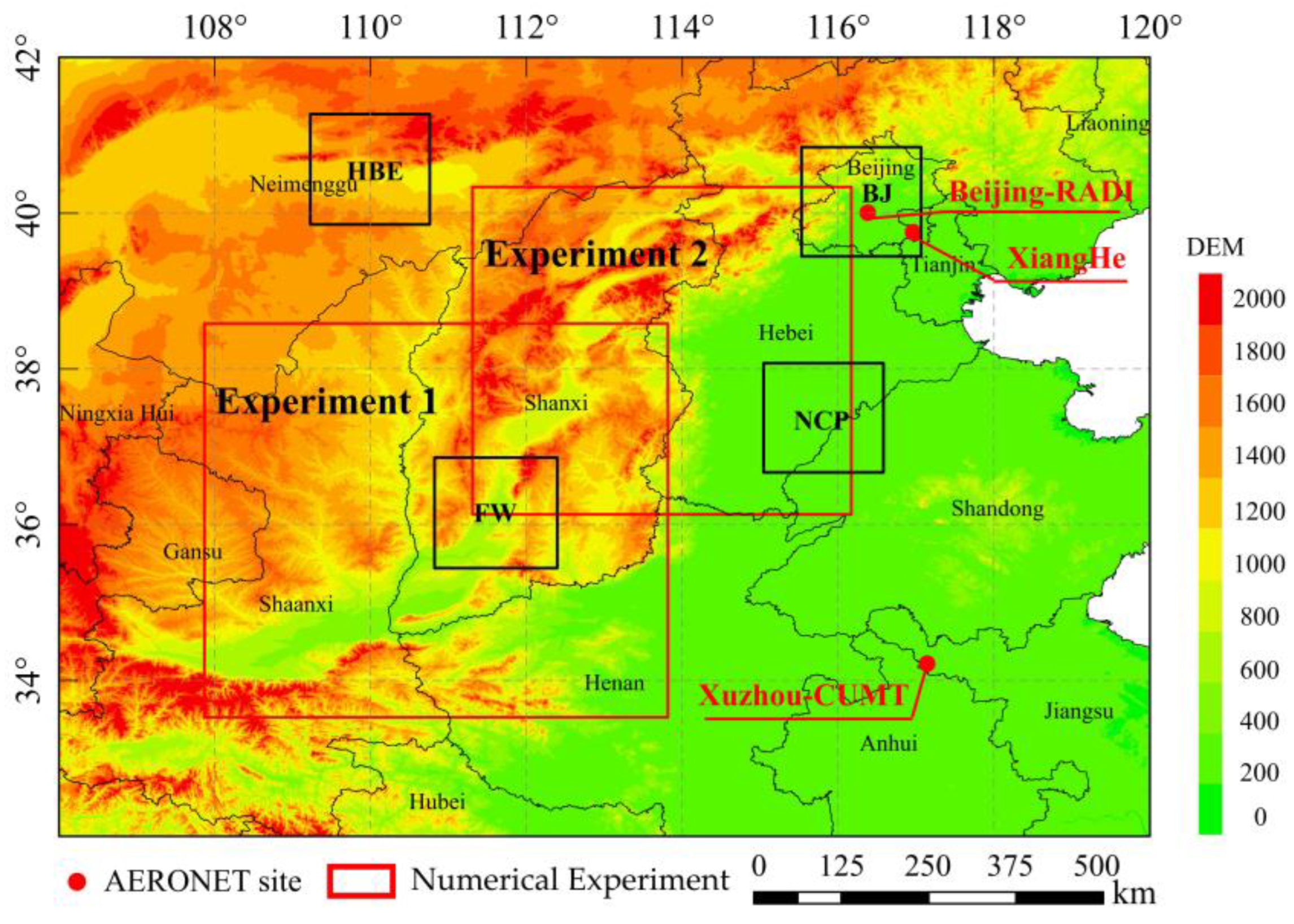
2.1. Study Area

Over the past three decades, China has experienced worsening air quality due to increased industrialization and urbanization. The North China Plain in particular is one of most polluted areas in the country, frequently experiencing heavy air pollution incidents, such as haze events [35] and ozone pollution [36]. Serious air pollution poses threats to production, life, and human health, including agricultural productivity [37], visibility deterioration [38], and premature death [39]. Therefore, this study focused on a square area in Northern China (32°N~42°N, 106°E~120°E) as the study area. Figure 1 represents four typical locations which were used for comparison with the topographic influences.

The two areas (Experiment 1 and Experiment 2) were additionally chosen for numerical experiments. Four regions were designed to demonstrate the correlation between the central pixel and the surrounding pixels, as well as the impact of the topography on it. First, the Hu–Bao–E urban agglomeration (HBE, 39.85–41.25°N, 109.25–110.75°E) was located in the Hetao Plain area to the south of the Yinshan Mountains, and its mean height is 1325.49 m. Second, Beijing (BJ, 39.45–40.85°N, 115.55–117.05°E), where the northwest is blocked by the Yanshan-Taihang Mountains, has a mean height of 392.38 m. Third, Fenwei Basin (FW, 35.45–66.85°N, 110.85–112.35°E) is the general name for the Fen River Valley and Wei River Valley, and the mean height is 1007.91 m. Fourth is a flat area of the North China Plain (NCP, 36.65–38.05°N, 115.05–116.55°E), where the mean height is 27.06 m.

2.2. Data and Method

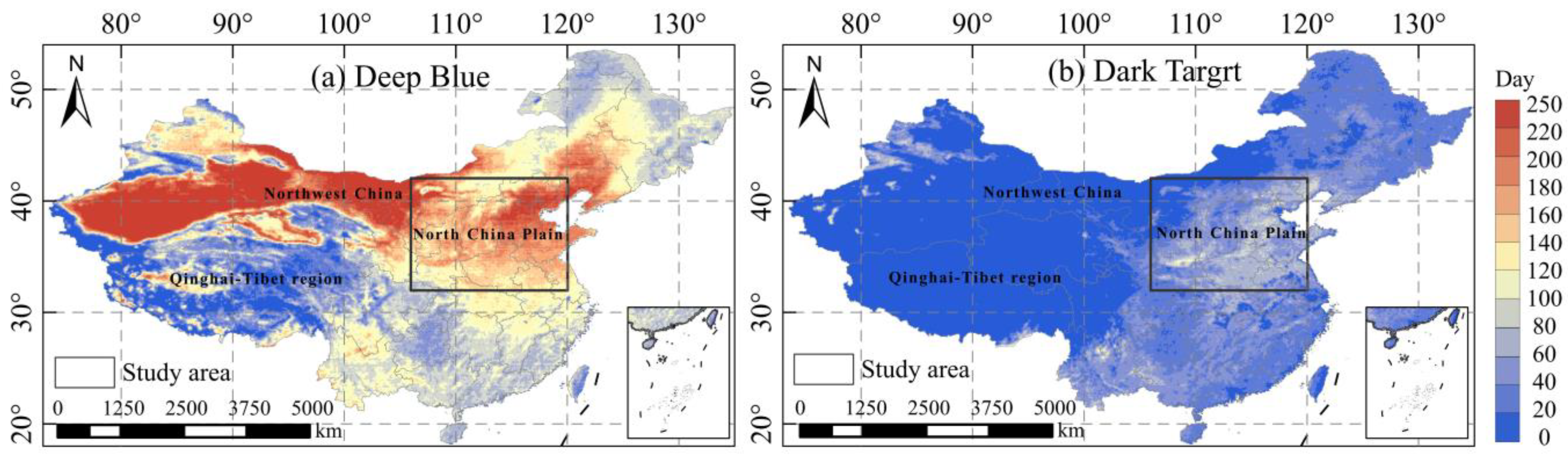
2.2.1. MODIS Data

The MODIS (moderate resolution imaging spectroradiometer) aerosol product monitors the ambient aerosol load and several properties of cloud-free and snow-free land and ocean aerosols. Collection 6.1 Dark Target (DT) and Deep Blue (DB) products [14] were obtained from the NASA Earth data search website (http://ladsweb.nascom.nasa.gov/ (accessed on 1 July 2019)) for this research. The spatial variability and differences in the AOD under heavy atmospheric pollution conditions can pose a challenge for accurate interpolation; as such, we selected the more polluted sample data for the algorithm. In China, the atmospheric conditions have improved significantly since 2016–2017 due to the atmospheric environmental management, and 2016 represents the year closest to the present with significant heavy pollution. Therefore, 10 km MODIS Aqua DT and DB data (MYD04) from the year 2016 over part of North China were chosen as the sample.

The DT algorithm screens the “dark pixel” targets with low surface reflectance and obtains the AOD by comparing the reflectance in the visible and near-infrared bands using the band ratio method [14]. The DB algorithm utilizes multi-band data, including the blue band that is sensitive to aerosol scattering and absorption, and applies inversion models to derive the results [40]. Figure 2 displays the number of the valid data days of the DT and DB in 2016. Since the DT AOD algorithm is mainly used in densely vegetated areas, the availability of a suitable time is limited. Coupled with cloud coverage, Figure 2a shows that the number of valid data days was less than the 100 in most areas and close to zero in the Tibet Plateau, Gobi, and desert regions of northwest China. In contrast, the DB AOD is useful for bright surfaces, and the valid data frequency was greater than 250 days in the northwest (Figure 2b). It was close to 200 days in the North China Plain, while due to the increasing cloud coverage moving southward, the frequency gradually reduced to less than 100 days.

2.2.2. AERONET Data

The Aerosol Robotic Network (AERONET) employs sun photometers to provide a dataset of AOD with low uncertainty (~0.01–0.02) [41] and high temporal resolution (~15 min) [42] under cloud-free conditions, by observing the extinction of the direct solar radiation through the aerosol-laden atmosphere. Although the reported wavelengths for the AOD may vary across different sites (and even for different periods within a specific site), almost all AERONET sites provide AOD at 440, 500, 675, and 870 nm at a minimum. AERONET represents a standard resource for validating [41,43] and bias-correcting the satellite AOD datasets [44,45], due to its high data quality, consistent processing standards, wide global range of sites, and free and easy access. AERONET Version 3 AOD data are computed for three data quality levels: Level 1.0 (unscreened), Level 1.5 (cloud-screened and quality-controlled), and Level 2.0 (quality-assured). In order to ensure data accuracy and an adequate amount of data, we chose to use Level 1.5 data for data validation.

The temporal average of all Level 1.5 AERONET AOD measurements within a ±30 min of the MODIS overpass time was calculated, as was the spatial average of all the MODIS AOD within a 25 km radius around the AERONET station [43].

2.3. Resample Method

For wide field spectroradiometers such as MODIS, there is a geometric distortion known as “the bow-tie effect” near the edge of the swatch. This effect results in across-track elongating up to ~4 times compared with the pixels near the center of the swatch. The 10 km resolution AOD products are also affected by this size increase and overlap [46]. When tools such as the HDF-EOS to GeoTIFF (HEG) [47] or MODIS Reprojection Tool (MRT) [48] are used to reproject and resample data, some errors may be introduced. However, this is aggregated at a basic pixel level (~10 km resolution), which may not be suitable for all users’ needs and requirements.

Therefore, a resampling procedure was proposed to convert the MODIS AOD HDF file to a GeoTIFF file (Figure 3). We resampled 10 km resolution MODIS AOD into a 0.05° spatial resolution (~5 km), which was more useful for spatial detailed information.

The steps included:

-

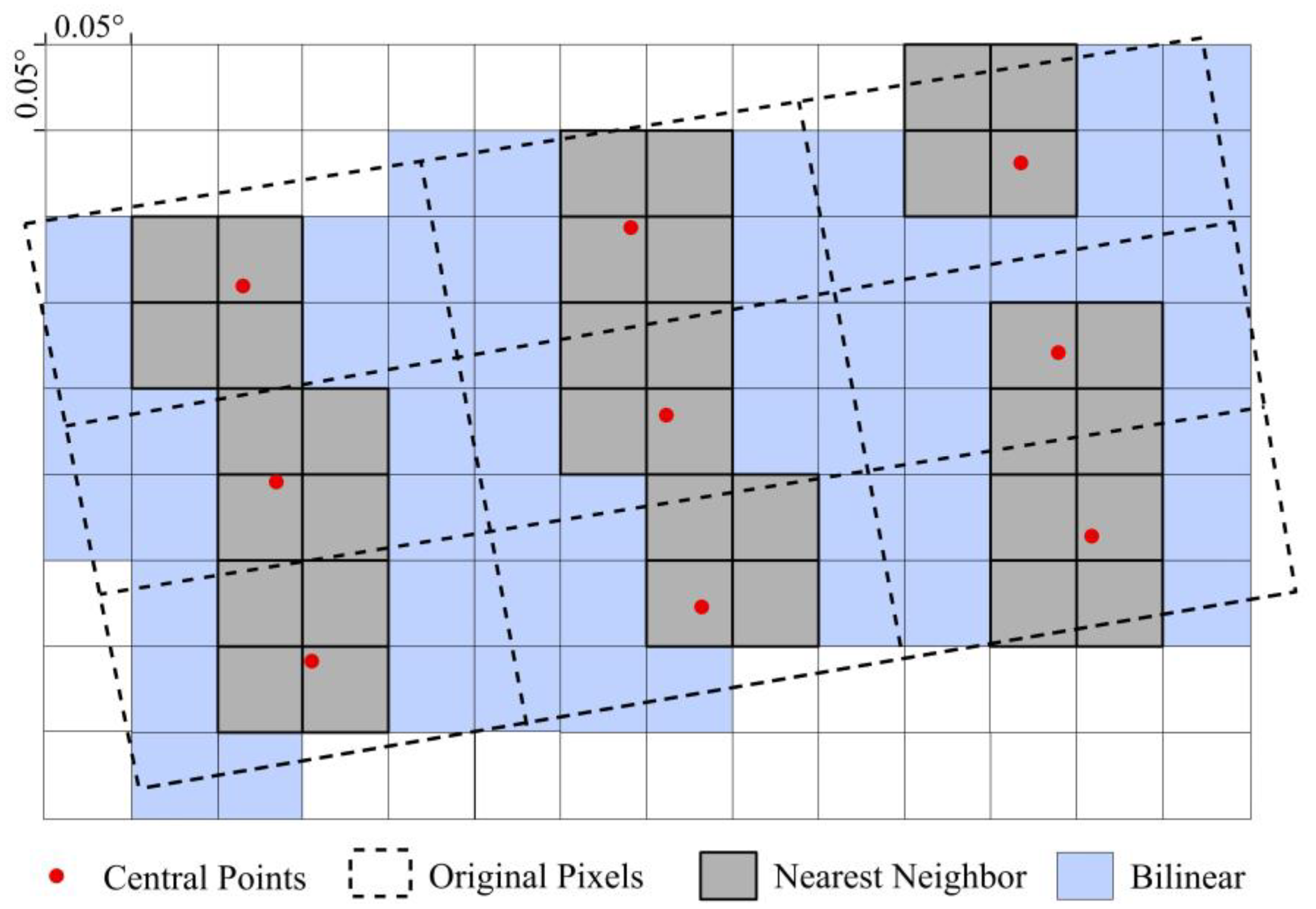
Constructing a grid with a 0.05° × 0.05° resolution.

-

Iterating through each pixel in the upper grid.

-

During the iteration, if a pixel was one of the four closest pixels to the central points (grey pixels), it was assigned the value from the nearest central point using the nearest neighbor method.

-

For pixels not in close proximity to the central points (blue pixels), a bilinear interpolation method was used to resample.

-

Ending after every pixel was processed.

After the above processing, the resampling results with a 0.05° resolution were obtained. When the field-of-view angle was small, most of the pixels were sampled using the nearest neighbor method, while bilinear interpolation was used only in the positions far from the center of the pixel with a large-field-of view angle.

2.4. ECW Interpolation Method

The AOD data generally exhibit higher similarity in regions with closer spatial proximity than in those with greater distances, but the correlation exhibits anisotropy. It is mainly determined by the fluidity characteristics of the atmosphere and the spatial distribution characteristics of the emission sources. While aerosols disperse freely in the atmosphere, they are also influenced by the prevailing winds and topography, leading to an uneven spatial distribution of atmospheric particles. In addition, the spatial distribution characteristics of particulate matter are mainly influenced by the distribution of emission sources, particularly anthropogenic sources, which are not uniformly distributed. Therefore, the spatial correlation of the AOD data in different regions presents various characteristics.

Figure 4a shows that the high values of the correlation coefficient were predominantly distributed in a longitudinal direction because of the limitations of the mountains on either side. Limited by the Yanshan-Taihang Mountains (Figure 4b), the correlation between the center pixel and the pixel in the northwest orientation was notably low, and a high correlation coefficient was observed in a northeast–southwest distribution pattern. Figure 4c shows a significant high correlation in the center of the basin, which rapidly decreases in higher altitude regions. Figure 4d shows the correlation coefficients were generally high in a flat area of the North China Plain, and they decreased with distance homogeneously.

Figure 4 illustrates that the correlation of the AOD values also influenced by topography and other factors, such as emission sources and atmospheric circulation. Therefore, the objective of this study was to extract the underlying spatiotemporal characteristics inherent in the AOD data to devise an appropriate interpolation technique tailored to the AOD data. Leveraging historical AOD data to formulate empirical correlation parameters, we employed these parameters as weighting factors in the interpolation process. Consequently, we termed this approach empirical correlation weighting (ECW).

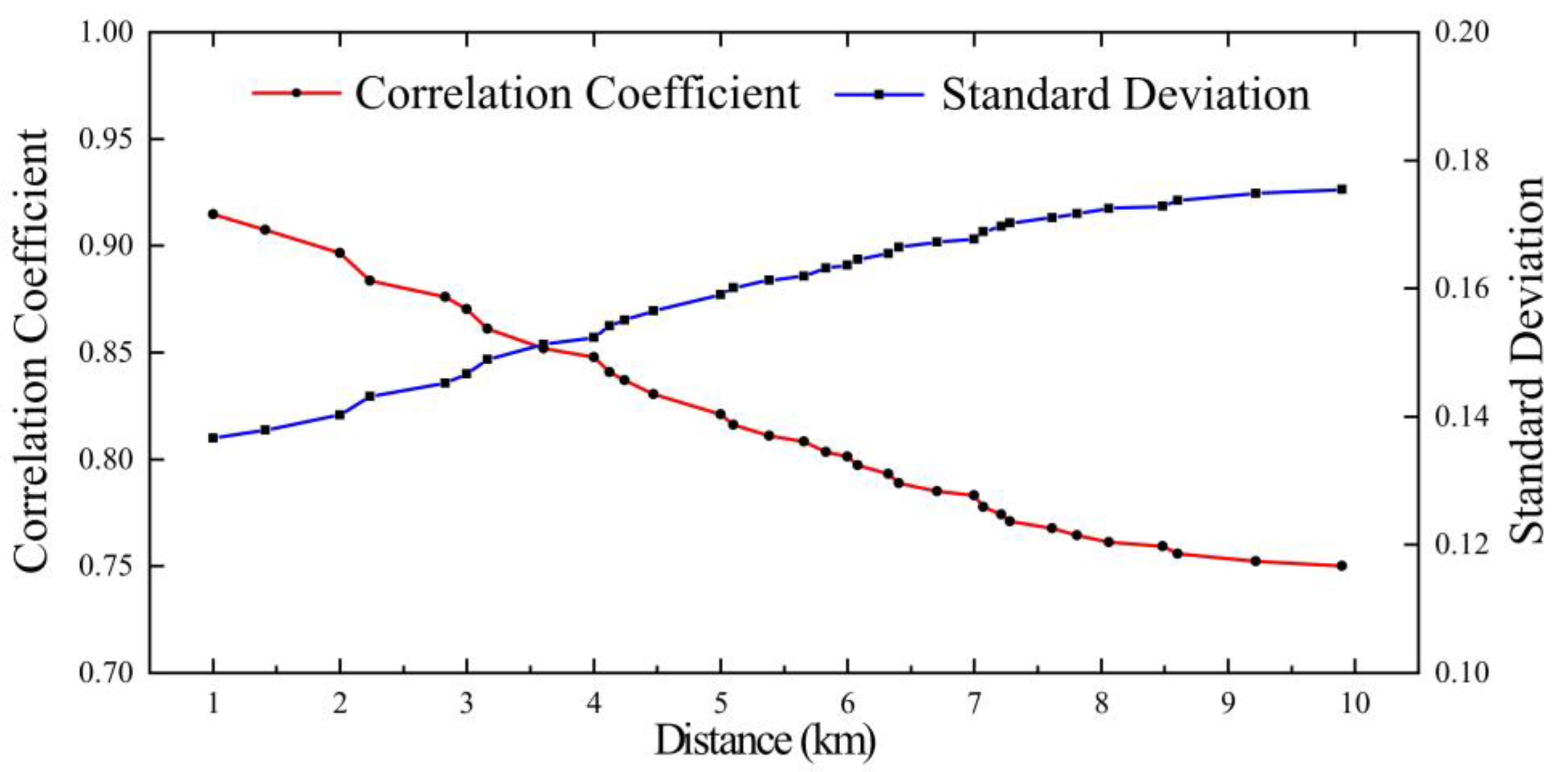
2.4.1. Slide Window Size Selection

Figure 5 depicts the relationship between the correlation coefficient and the distance, the average result obtained from calculating the correlation between all pairs of points within the study area in the 2016, and the distance represents the distance between the central pixel and the outermost pixel. These show that the correlation coefficient gradually decreased as the distance increased, while the standard deviation increased. Considering both the correlation and its stability, we assumed that a correlation coefficient of 0.8 was suitable for interpolation, the interpolated range was 60 km, and the standard deviation was approximately 0.15.

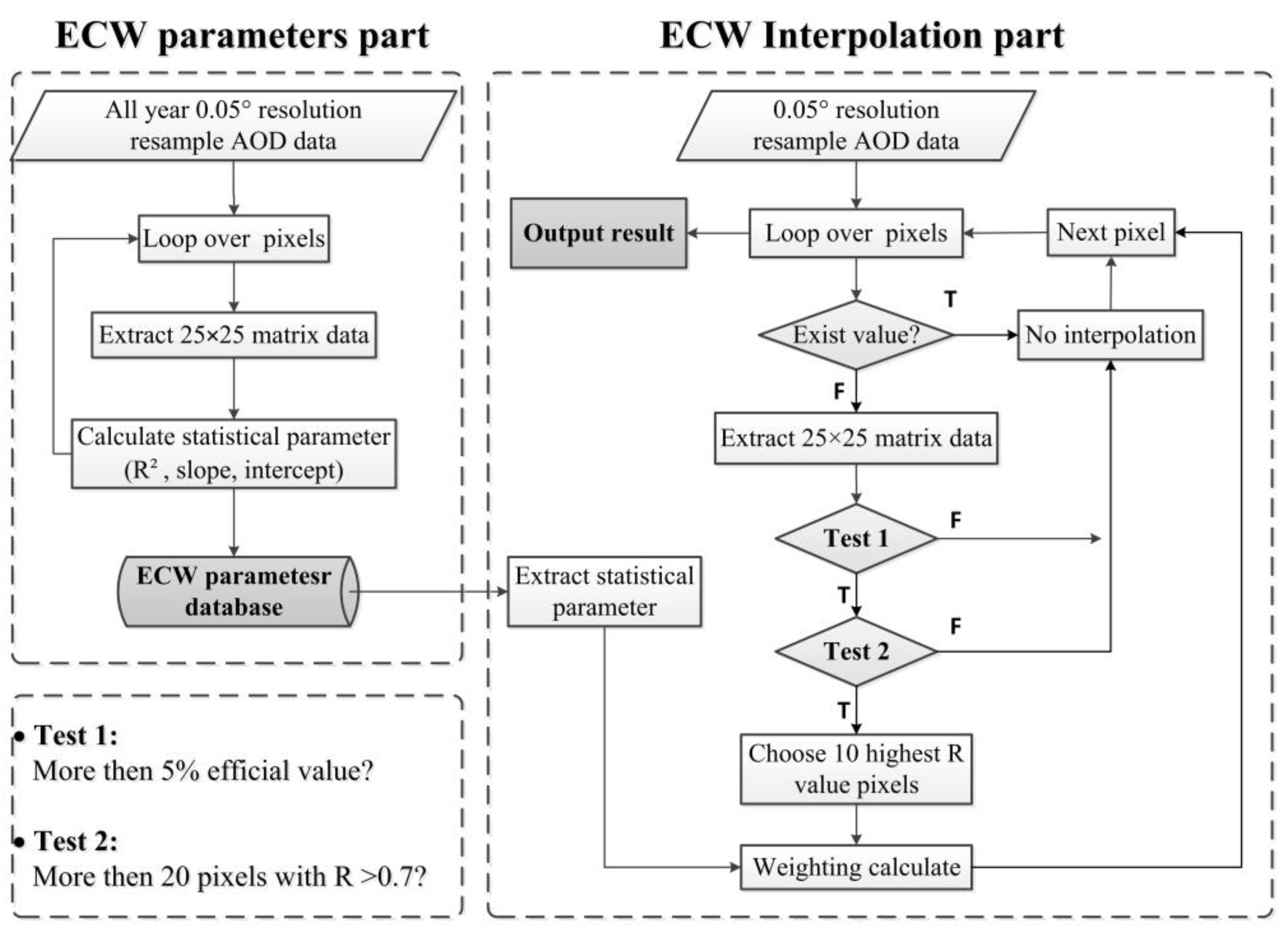
2.4.2. Establishment of the Correlative Look-Up Table (LUT)

Since the interpolated results are not completely accurate, we constructed the lookup table using only the original AOD data. The look-up tables were pre-calculated for each parameter, where the correlation coefficient served as the weight, and the linear regression coefficient was used as the correction coefficient. The process of establishing the LUT was as follows:

-

Resampling the AOD data from HDF files to 0.05° products; MODIS data may contain overlapping observations of mid–high latitudes at different time points within a day. The two observations were averaged to obtain the observed values for the overlapping coverage area.

-

Looping over all pixels, extracting a 25 × 25 matrix (representing points remote from the area’s center no more than 60 km, which was equivalent to about 12 pixels at the 0.05° resolution) of AOD data centered on each pixel for the year of 2016.

-

Matching the AOD value at the center pixel with that of the surrounding 624 (=25 × 25 − 1) pixels, discarding the invalid value; the cases in which the center pixel and the surrounding pixel had values at the same time were selected as the sample pairs.

-

Calculating the statistical parameters (correlation of determination (R²) , slope, and intercept of the linear regression) for each of the sample pairs.

-

Processing every pixel and storing the statistical parameters.

-

Building an LUT of a four-dimensional array (column, row, 624, 3).

2.4.3. Interpolation Strategy

Then, the LUT was applied to the AOD interpolation. The steps are illustrated in the ECW interpolation part of Figure 6, and the detailed strategy was as follows:

-

Looping over every pixel of the AOD resampled image and performing interpolation for the non-valued pixels.

-

For a non-valued pixel, determining whether the number of valued pixels within the sliding window (25 × 25) centered on the pixel was greater than 5% (25 × 25 × 0.05 = 31); if there were less than 31 pixels, the surrounding information was deemed insufficient, and it is difficult to give enough information, no interpolation was performed, and we proceeded to the next pixel.

-

Extracting the information about the central pixels from the LUT and matching the information from the valued pixels; the number of pixels with an R greater than 0.7 was checked, and if there were more than 20 pixels, we proceeded to the next step. If there were not more than 20 pixels, the number of surrounding highly correlated pixels was insufficient, there was not enough information for interpolation, and we moved on to the next pixel.

-

Selecting the 10 pixels with the highest R for the weighting calculation to avoid the overfitting of parameters; these values were revised according to the linear regression equation and then weighted using the weights of the R². The formula is as follows:

$${\mathrm{A}\mathrm{O}\mathrm{D}}_{\mathrm{E}\mathrm{C}\mathrm{W}}=\sum _{\mathrm{i}=1}^{10}{\mathrm{R}}_{\mathrm{i}}^2\times \left({\mathrm{A}\mathrm{O}\mathrm{D}}_{\mathrm{i}}\times {\mathrm{s}\mathrm{l}\mathrm{o}\mathrm{p}\mathrm{e}}_{\mathrm{i}}+{\mathrm{i}\mathrm{n}\mathrm{t}\mathrm{e}\mathrm{r}\mathrm{c}\mathrm{e}\mathrm{p}\mathrm{t}}_{\mathrm{i}}\right)/\sum _{\mathrm{i}=1}^{10}{\mathrm{R}}_{\mathrm{i}}^2$$

(1)

-

Repeating the above steps until all pixels were calculated.

In Equation (1), ${\mathrm{A}\mathrm{O}\mathrm{D}}_{\mathrm{E}\mathrm{C}\mathrm{W}}$ represents the interpolated results of the ECW method, i represents the number of pixels available for interpolation, ${\mathrm{A}\mathrm{O}\mathrm{D}}_{\mathrm{i}}$ is the valid value that can be used to interpolate, and the ${\mathrm{R}}_{\mathrm{i}}^2$, ${\mathrm{s}\mathrm{l}\mathrm{o}\mathrm{p}\mathrm{e}}_{\mathrm{i}}$, and ${\mathrm{i}\mathrm{n}\mathrm{t}\mathrm{e}\mathrm{r}\mathrm{c}\mathrm{e}\mathrm{p}\mathrm{t}}_{\mathrm{i}}$ are statistical parameters.

2.5. Validation Method

2.5.1. Estimation Validation

Satellite data, being dense raster data, differ from discrete point data obtained from a meteorological station. Validating the interpolation effect on a large scale becomes challenging. Therefore, we chose two numerical experimental areas for the estimation and validation of the interpolation results. The experimental areas were chosen in the part of the terrain with complex topography and highly spatially detailed information. In order to ensure a sufficient amount of data and the sample amount for validation in the experimental areas, each experiment was selected to have relatively complete data for validation on five days in each month. The validation included single day validation and overall validation. Single-day validation was the validation of the actual and interpolated resultant values for each day, as well as the calculation of the quarterly and yearly averages. The overall validation collected all the actual and interpolated values from the experimental area to avoid the bias caused by small amounts of data. The accuracy and stability of the ECW model’s predictions were evaluated based on the rank correlation coefficients (${\mathsf{\rho }}_{\mathrm{R}}$) [49], R², mean absolute error (MAE), and root mean square error (RMSE).

2.5.2. Validation with AERONET

To validate the reasonableness of the accuracy of interpolated data, AERONET data were utilized for comparison and validation in this study. Three AERONET sites, namely Xianghe, Beijing–RADI, and Xuzhou–CUMT, provided complete annual observation data for 2016 within the AERONET experimental area. While MODIS provides AOD data captured at the sensor imaging time, AERONET provides AOD measurements from different stations at a time resolution of 15 min, resulting in different time resolutions. To ensure the reliability and accuracy of the validation, the satellite data in this study were centered around the observation site and averaged within a 25 km radius [43], at least 40% of valid values [50]. The ground data were averaged over a period of half an hour before and after the satellite transit moment. Lastly, AOD point pairs of the interpolation value and real value were obtained.

3. Results

3.1. Numerical. Experimentation

Two sets of actual data were selected for numerical experiments to visually show the effects of different interpolation methods before the specific analysis. The selected actual satellite observation data meet the high coverage of the region, complex terrain, and spatial detail information. A wider range of values was artificially eliminated to simulate missing observations. Interpolation was performed using different interpolation methods in the artificially eliminated area at 0.05° resolution, and the interpolation results were compared with the original true values. Figure 7 represents the regional data from the Experiment 1 (Figure 1) on 5 November 2016. Figure 8 represents the data from the Experiment 2 (Figure 1) on 12 November 2016.

In Experiment 1 (Figure 7), the original AOD high value area was mainly concentrated in the southwest Fenwei basin and extended from the southwest to northeast, and the AOD value exhibited a discontinuous pattern in the extended direction. The artificially eliminated areas were long elliptical regions, and most of the high-value areas were removed while retaining other high values in the southwest and south. Figure 7c–e show the interpolation results of the ordinary Kriging (OK), TPS, and ECW interpolations, respectively. The results suggest that the three methods generally recovered the distribution of the high AOD value, while two conventional interpolation methods exhibited deficiencies in capturing the spatial detail of the AOD distribution. In contrast, the ECW interpolation performed better in reproducing the spatial detail distribution characteristics that closely resembled the actual observations. Specifically, in the central part of the basin, the high-value zone maintained a distribution relatively close to the original data in the ECW. Although the OK and TPS restored the high-value zone, there were also excessive high-value distributions and boundary blurring, especially in the northeast extension direction. Both the TPS and OK failed to effectively represent a significant transition. The interpolated area in Figure 7 exhibits a flat topography and high spatial correlation within the basin’s interior. As the distance from the center of the basin increased, the spatial correlation gradually decreased, with the surrounding mountains acting as the boundary of the region. Due to the spatial correlation of the AOD and the characteristic of matching the topography, the AOD values spread from high to low from the center of the basin outward.

In Experiment 2 (Figure 8), the spatial distribution of the original AOD data was characterized as high values in the east and low values in the west, with a clear demarcation between the two regions. Between them, there was a distinct bulge in the region, where the high AOD values transitioned to low values. Bulge areas were deliberately eliminated to test the performance of different interpolation methods under this situation. The results showed that both the OK interpolation and TPS interpolation failed to recover the high value region of bulge part. The ECW interpolation result captured the spatial distribution details of the bulge region, and interpolated clear boundaries, although the high values were not high enough. Due to the influence of the topographic factors, there is a spatial correlation on the eastern side of the boundary where air cannot easily diffuse, resulting in a concentrated distribution of AOD. On the west side of the boundary, under the influence of topographic barriers, the spatial correlation decreases. These results reflect the correlation of the AOD with the topography.

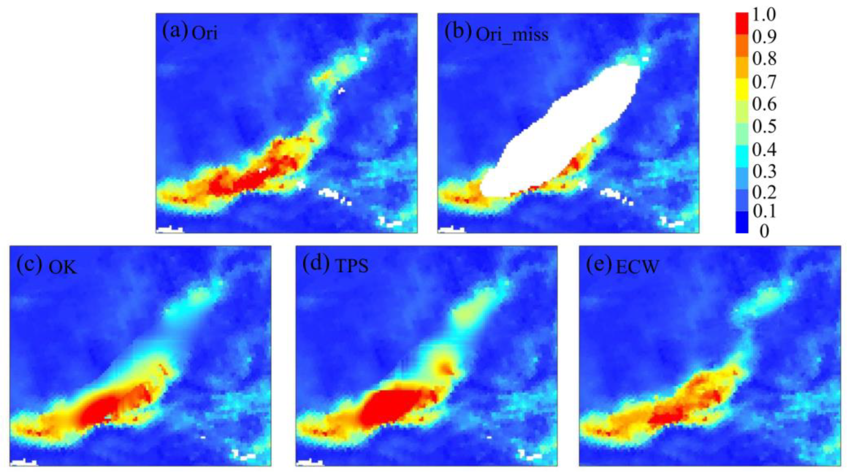
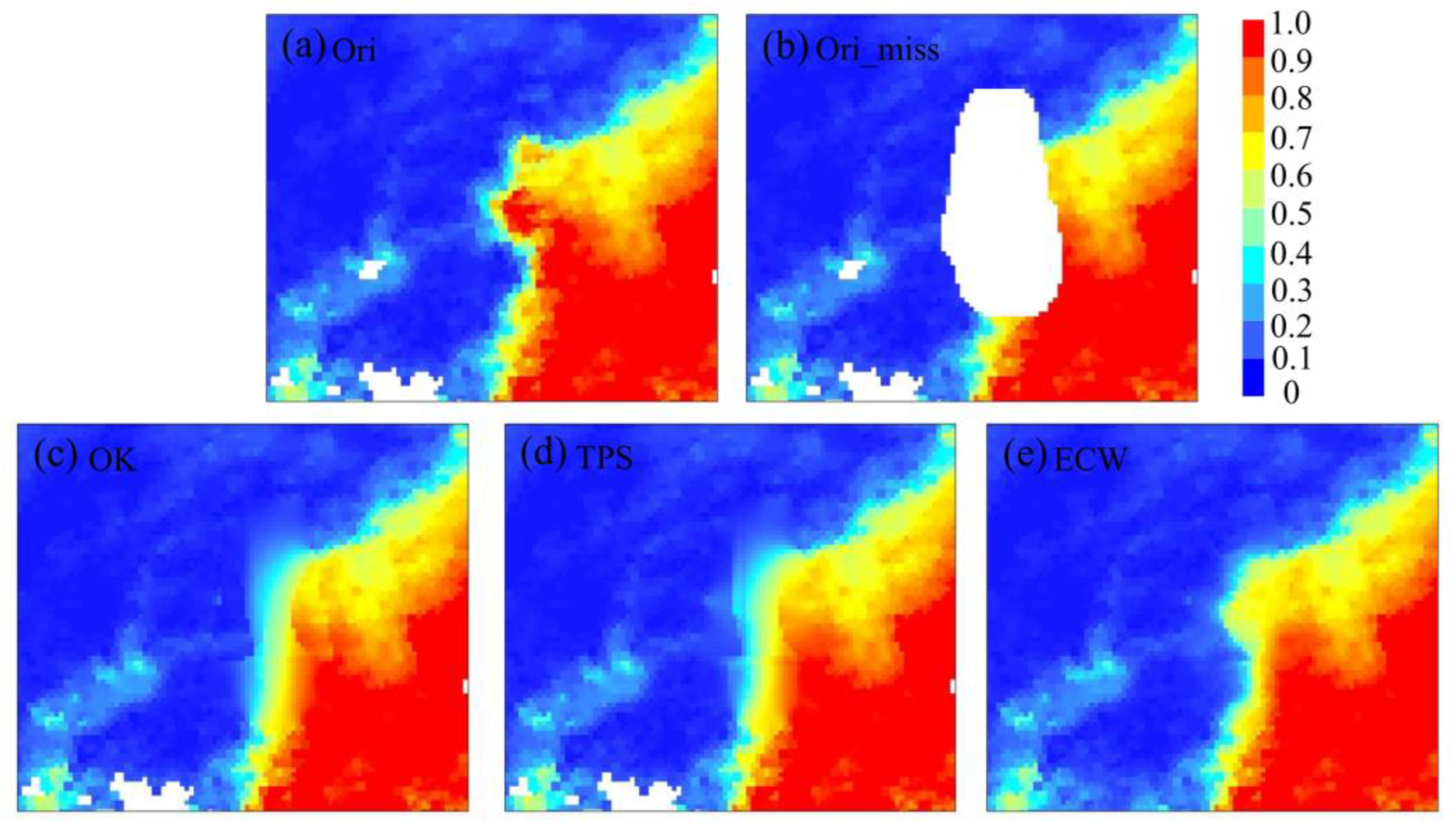
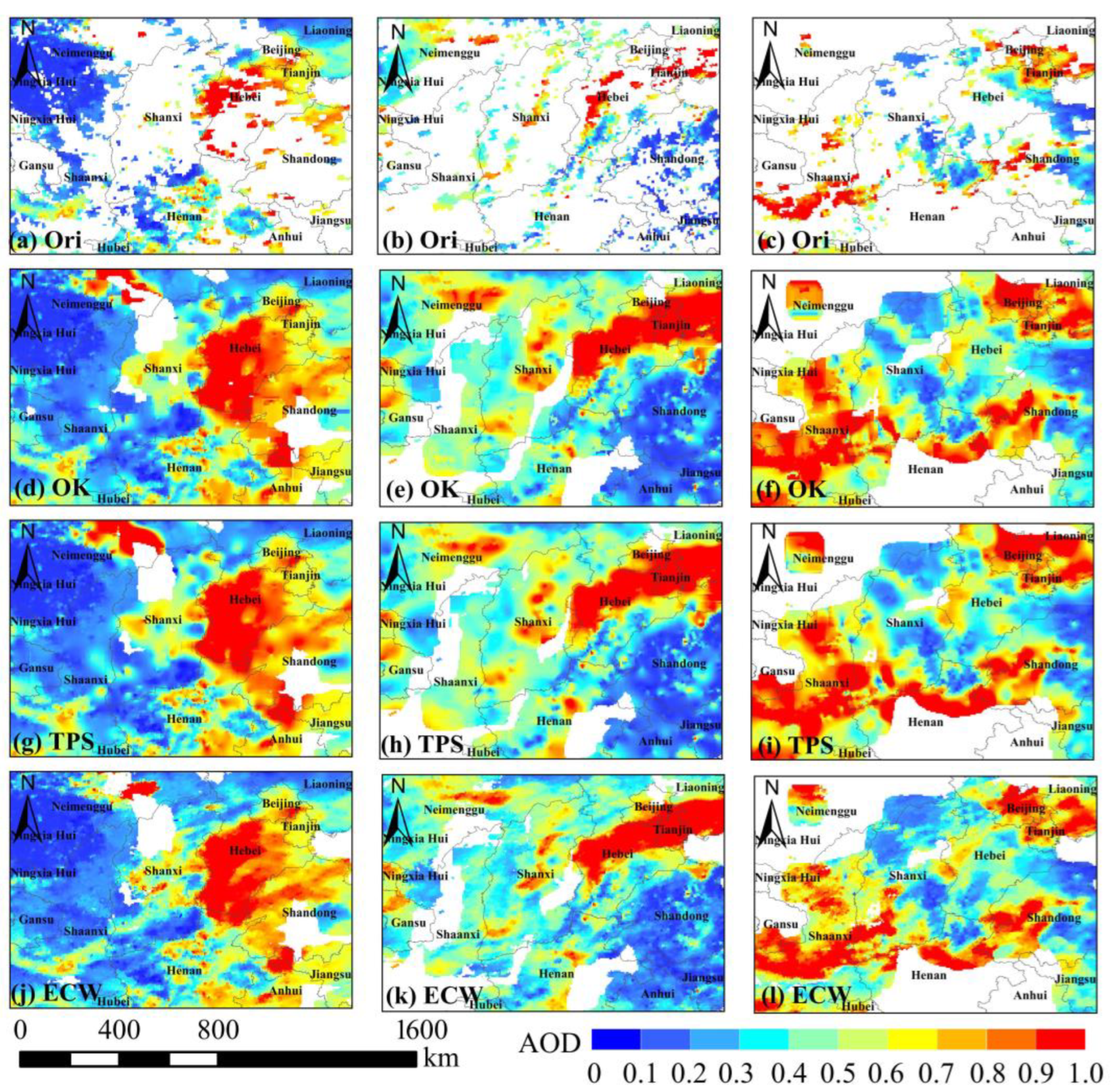
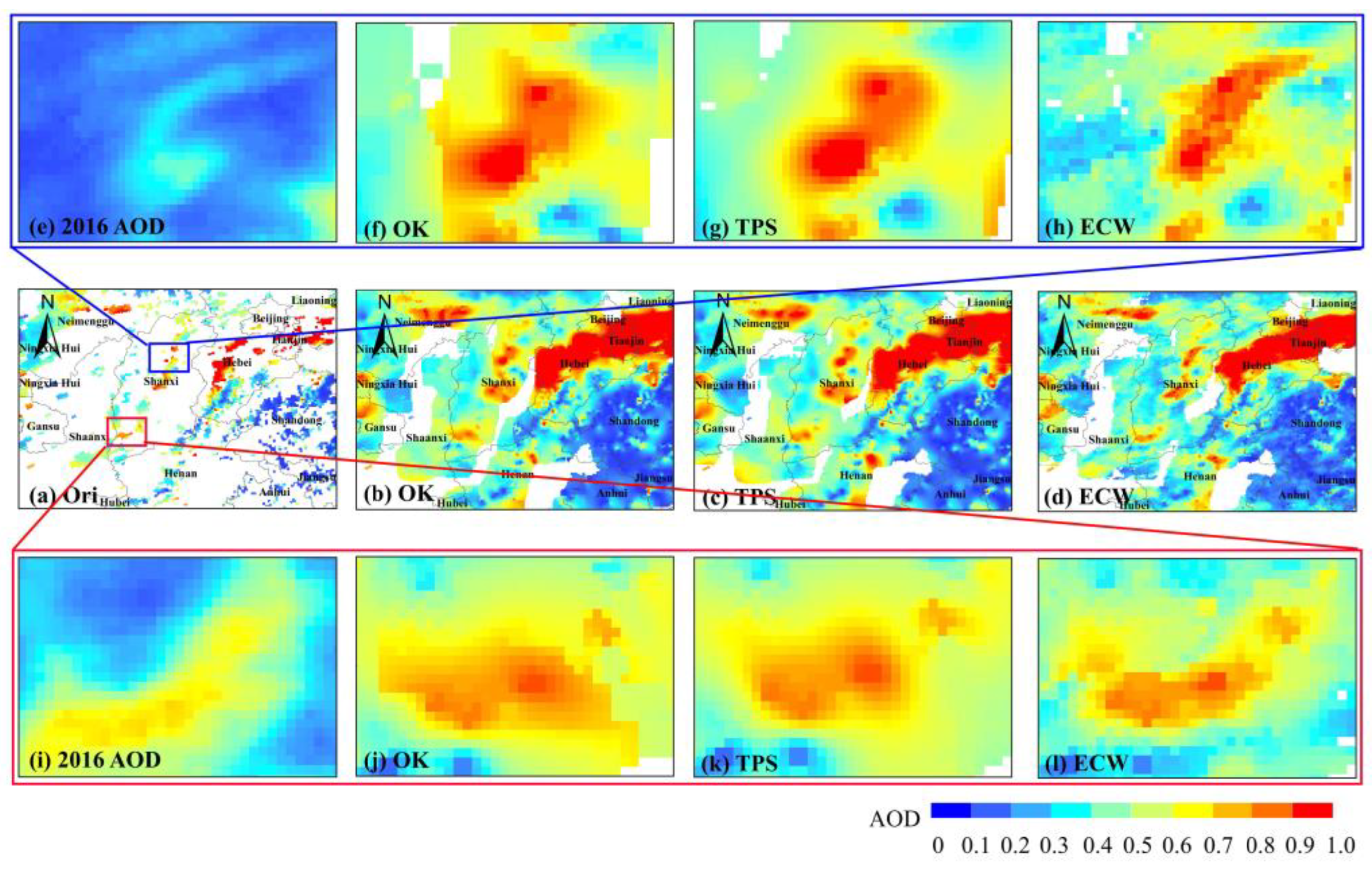
3.2. Cases Comparison and Analysis

Three actual interpolation cases (18 May, 10 August, and 22 August 2016) were selected for visual comparison to assess the interpolation effect (the display area in the Figure 9 shows the study area with 12 pixels removed from the edge). All three days were chosen with a principle of low and fragmented data coverage to demonstrate the effectiveness of the interpolation methods. Figure 9 illustrates the results of the three interpolation methods. It can be observed that the three methods successfully recovered the spatial distribution of the AOD over a large range using the limited observation data. Some areas were empty due to their significant distance from the valid value. We must reiterate that we do not to achieve gapless interpolation, because even if we can achieve it for distant locations, the reliability of these results would be questionable.

Meanwhile, we visually analyzed the spatial distribution of single-day interpolation results based on the spatial distribution of mean results for the year 2016. A detailed comparison (Figure 10) was conducted from Figure 9b to explain the advantage of the ECW method. The OK and TPS interpolation results exhibited a noticeable halo phenomenon, with the interpolation results expanding outward from the central high value point. However, this expansion failed to conform to the flow field characteristic. Comparing the mean value results for the whole year of 2016 (Figure 10e–i), the spatial characteristics of the ECW interpolation were consistent with them. They also exhibited clear directional characteristics rather than simple outward expansion.

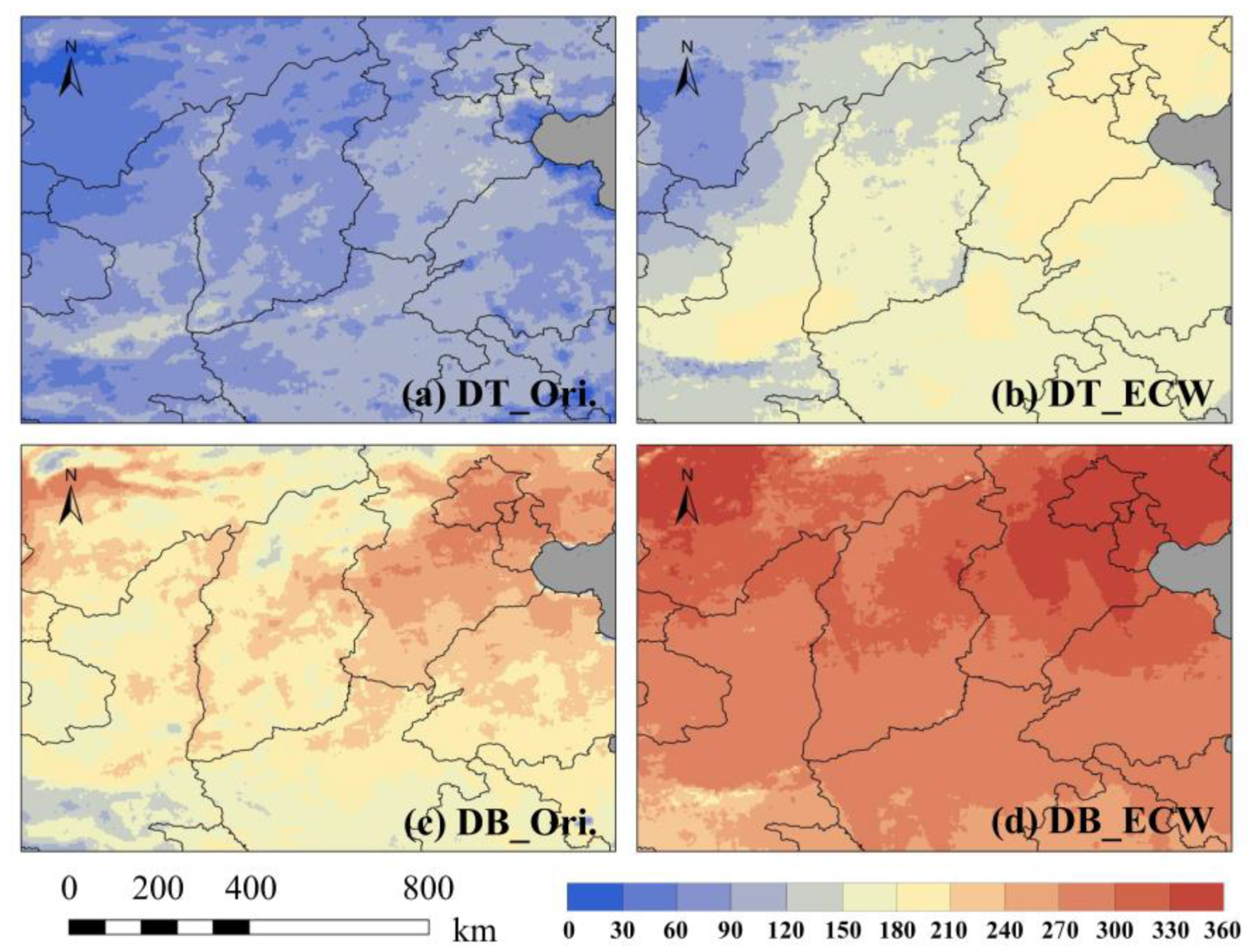
3.3. Spatial and Temporal Coverage

First, the spatial coverage (number of effective pixel points/number of all pixel points) of the daily satellite data in the experimental area was calculated; then, the results were averaged on a monthly scale as shown in

Table 1. The spatial coverage percentage of the original data and the ECW results over our research region.

Month	DB			DT
	Origin	ECW	Difference	Origin	ECW	Difference
January	46.07%	70.64%	24.57%	4.42%	6.99%	2.57%
February	46.07%	74.71%	28.64%	6.04%	16.26%	10.22%
March	52.81%	75.58%	22.76%	11.23%	26.57%	15.33%
April	50.50%	69.08%	18.58%	16.79%	37.76%	20.97%
May	44.37%	63.89%	19.52%	19.53%	39.37%	19.84%
June	39.97%	73.53%	33.56%	29.08%	53.20%	24.12%
July	45.89%	67.01%	21.11%	17.35%	41.58%	24.23%
August	34.43%	69.28%	34.85%	14.88%	41.00%	26.12%
September	32.30%	72.85%	40.56%	25.75%	53.05%	27.30%
October	44.41%	62.25%	17.85%	16.41%	33.46%	17.05%
November	33.93%	73.97%	40.04%	15.35%	32.78%	17.43%
December	55.84%	75.04%	19.20%	3.70%	9.40%	5.70%
Total	43.88%	70.65%	26.77%	15.04%	32.62%	17.57%

. The original DB product had a monthly average spatial coverage ranging from 32.30% to 55.84%, with a mean value of 43.88%. After ECW interpolation, the spatial coverage improved by approximately 17.85% to 40.56%, with an average improvement of 26.77%. The annual average spatial coverage reached 70.65%. The improvement in data coverage for the DB product was more stable because the algorithm could be affected by the characteristics of the underlying surface and was primarily influenced by cloud interference. As for the DT product, there were obvious seasonal characteristics in its original data spatial coverage. It had less interpolation data in winter due to the withered vegetation, but more data in other seasons, although it still had fewer data compared to the DB product. On average, the annual spatial coverage of the original DT product increased from 15.04% to 32.64% after interpolation.

The ECW interpolation effectively improved the spatial coverage of the data. The algorithm makes no attempt to implement global interpolation, but only interpolates within a maximum distance of 0.6° from each pixel that meets the necessary conditions, resulting in non-seamless results. By improving the spatial coverage of individual daily images, the frequency of the effective observations for each pixel throughout the year also increases. Figure 11 displays the spatial distribution of the number of effective observation days in 2016. The coverage days of the DT products improved from less than 90 days to generally exceeding 150 days. The improvement in the DB product was more prominent, with high areas reaching close to 200 days. After interpolation, the coverage days generally increased to approximately 300 days, and some areas even approached 100% coverage. The interpolation of both data products using the ECW has led to significant improvements. The DB product achieved a time coverage of nearly 300 days, which reduced the bias in the mean value calculation and made the mean product more representative.

3.4. Validation

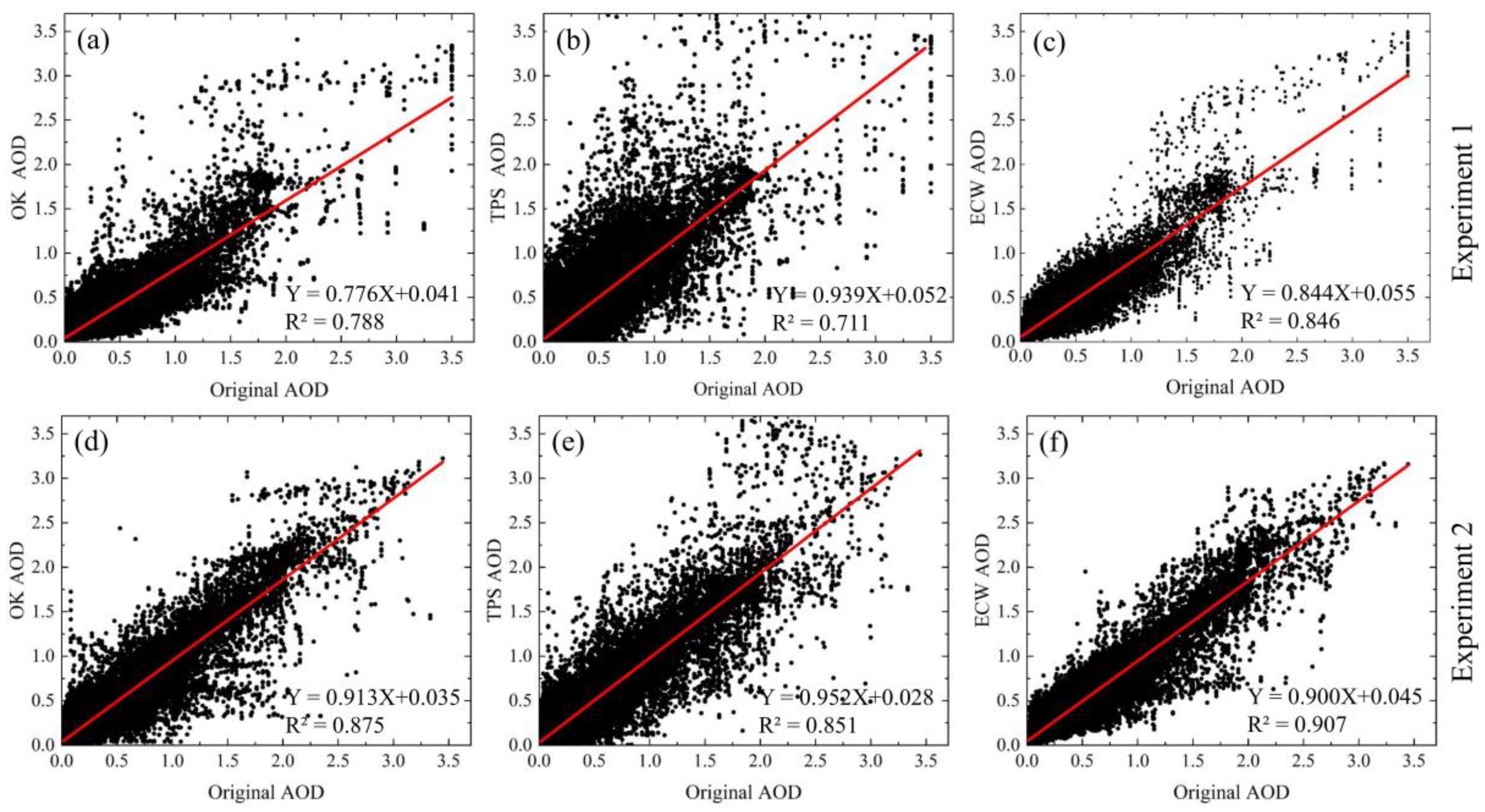
3.4.1. Estimation Validation

For a reliable and statistically significant comparison, the regions with a richer data volume for 5 days in each month were selected for artificial elimination and interpolation. The ${\mathsf{\rho }}_{\mathrm{R}},$ R², RMSE, and MAE were computed separately for the quarterly and yearly mean methods (

Table 2. Quarterly and annual statistical parameters of the numerical experiments.

Season	Method	Experiment 1				Experiment 2
		${\mathsf{\rho }}_{\mathbf{R}}$	R2	RMSE	MAE	${\mathsf{\rho }}_{\mathbf{R}}$	R2	RMSE	MAE
Spring	OK	0.7257	0.5427	0.1551	0.1075	0.8074	0.6683	0.0963	0.0684
	TPS	0.7118	0.5024	0.1832	0.1229	0.7857	0.6494	0.0971	0.0687
	ECW	0.8284	0.6782	0.1305	0.0923	0.8220	0.6794	0.0956	0.0702
Summer	OK	0.7014	0.5390	0.1606	0.1031	0.7801	0.6780	0.1647	0.1125
	TPS	0.6698	0.4638	0.1986	0.1272	0.7799	0.6445	0.1906	0.1317
	ECW	0.8080	0.6427	0.1439	0.0962	0.8353	0.7087	0.1554	0.1078
Autumn	OK	0.7714	0.6255	0.1112	0.0783	0.8257	0.7423	0.1429	0.0978
	TPS	0.7328	0.5382	0.1499	0.0985	0.8342	0.7186	0.1698	0.1138
	ECW	0.8662	0.7234	0.0991	0.0690	0.8808	0.7859	0.1259	0.0863
Winter	OK	0.8013	0.6600	0.1066	0.0746	0.7735	0.6613	0.1284	0.0828
	TPS	0.7831	0.6298	0.1305	0.0865	0.7850	0.6649	0.1247	0.0755
	ECW	0.8765	0.7723	0.0950	0.0663	0.8500	0.7208	0.1078	0.0707
Year	OK	0.7499	0.5918	0.1334	0.0909	0.7967	0.6875	0.1331	0.0904
	TPS	0.7244	0.5335	0.1655	0.1088	0.7962	0.6694	0.1456	0.0974
	ECW	0.8448	0.7042	0.1171	0.0809	0.8470	0.7237	0.1212	0.0838

). The results showed that the ECW obtained the highest ${\mathsf{\rho }}_{\mathrm{R}}$ and R² and the lowest RMSE and MAE in yearly mean results. Specifically, in Experiment 1, the ${\mathsf{\rho }}_{\mathrm{R}}$ and R² of the ECW were 0.8448 and 0.7042, and the RMSE and MAE were 0.1171 and 0.0809, respectively. In Experiment 2, the ${\mathsf{\rho }}_{\mathrm{R}}$ and R² of the ECW were 0.8470 and 0.7237, and the RMSE and MAE were 0.1212 and 0.0838, respectively. The same results were true for summer, autumn, and winter. In Experiment 2, the OK obtained the lowest MAE (0.0684) in spring. Overall, between the two numerical experiments, the interpolation results of Experiment 2 were closer to the true values and had a higher overall accuracy. However, the validation results of the seasonal mean and annual mean of the two experiments were similar, and the accuracy of the interpolation method was ECW > OK > TPS.

In order to avoid the effect that the bias of a small amount of data has on the mean value, we validated all the interpolated results of the two numerical experiments. The scatter diagrams (Figure 12) between the interpolated results and the original values in the artificially eliminated areas demonstrate the advantages of the ECW method. TPS interpolation acquired the lowest R² of 0.711 and 0.851 in both experiments. The R² values for the ECW were 0.846 in Experiment 1 and 0.907 in Experiment 2. Compared with the other two methods, the ECW performed well in interpolation accuracy. In particular, in Experiment 1, the overestimation of the ECW was more pronounced at high values of AOD (>2.0), while the OK and the TPS also showed more pronounced overestimation at low values.

3.4.2. AERONET Validation

AERONET data were applied to the accuracy validation of the interpolation results. Limited by the sun photometer observation mode and the presence of clouds, ground-based observations were constrained. Therefore, there was a lack of valid ground-based observations that matched the interpolation results, resulting in a limited increase in the number of samples. We integrated the matched data from three sites (Xianghe, Beijing-RADI, Xuzhou-CUMT) for computation (Figure 13). The results indicated that the increase in data points for DT and DB AOD went from 152 and 416 to 251 and 440, respectively, with DT AOD showing a more significant increase. There were no significant differences in accuracy among the three interpolation methods. In DT AOD, the R for ECW and OK were the same, but ECW had slightly lower RMSE and MAE compared to OK. For DB AOD, ECW and TPS had the same R values, but ECW had slightly higher RMSE and MAE compared to TPS. Overall, the interpolated data with ECW maintained a relatively high level of accuracy. In DT and DB AOD, R decreased by 0.04 and 0.006, while RMSE and MAE increased by 0.063 and 0.007, 0.018 and 0.008, respectively.

4. Discussion

Based on the spatial correlation of the atmospheric data and considering the directional characteristics of the correlation due to the emission sources, wind fields, and topography, historical data were used to describe this feature, and we proposed an ECW method to interpolate the satellite AOD data. In this study, meteorological, topographic, and emission source factors were utilized to analyze the spatial distribution characteristics of AOD. Our aim was not to analyze their influence on the distribution or quantify their contributions. Instead, this study focused on elucidating the statistical characteristics of the spatiotemporal distribution of AOD in the presence of these influencing factors.

Due to various factors, AOD data also exhibit seasonal variations. When constructing the LUTs, employing quarterly data may better capture the spatiotemporal information. However, there is a notable absence of MODIS DT and DB data, particularly in the DT product. This makes LUTs calculations based on quarterly data potentially unstable. Therefore, we opted to construct the LUTs using one year of historical data and calculated interpolation results. Regarding the problem of the interpolation range, we did not aim to produce seamless aerosol data products. All the interpolation methods relied on the principle of the spatial correlation of the data. Our statistical results showed that the spatial correlation of the AOD data decreased as the distance increased, and thus, only interpolation results within a certain range hold meaningful information. Imagine a common scenario where a layer of clouds covers land over 2000 km in diameter. Meanwhile, the AOD value at a location beneath the center of the cloud is interpolated using observational data collected from thousands of kilometers away. In this context, to what extent can we have confidence in the accuracy of this estimated value?

The ECW method proposed in this study yields valid and accurate interpolation results. For the DT and DB data, the interpolated results significantly improved the average spatial coverage to 32.62% and 70.65%, respectively. The missing data for the DT algorithm were mainly due to the sparse vegetation on the underlying surface and the presence of clouds; hence, a relatively low number of valid observations for interpolation were obtained. The DB algorithm has better applicability to different underlying surface conditions, and the missing interpolation was mainly caused by cloud cover. Therefore, the DT interpolation fills in the aerosol results, not only under clouds but also in non-dense vegetation areas, while the enhanced spatial coverage was not significant due to the limited number of originally valid observations. On the contrary, the results after the DB interpolation effectively filled in the aerosol values under cloud and improved the spatial coverage due to a larger number of original valid observations. After improving the spatial coverage of daily observations, the number of effective observation days throughout the year was significantly increased (e.g., more than 300 effective days for most regions with DB interpolation). The higher sampling proportion is helpful to make the time-averaged results more representative.

This study employed two methods to validate the interpolation method. In the estimation validation, two regions with complex terrain, rich spatial information, and abundant original data were selected for artificial elimination and interpolation calculation to verify the accuracy and reliability of the interpolation results. The validation results effectively demonstrated that ECW can still produce relatively accurate results in various interpolation challenges. To further confirm that our interpolated results maintain relatively high data accuracy, we conducted validation using AERONET site data. Since the missing data of the DT algorithm were influenced by the surface conditions, the increase in the matched data after interpolation was significantly greater than that of DB. The validation results also continued to exhibit relatively high accuracy with only a minimal increase in errors. However, it is important to note that this validation method suffered from a limitation in the form of a limited increase in matched data points after interpolation. This limitation primarily stemmed from the lack of ground-based observation support. Therefore, the use of longer time series data and data from a larger number of sites would be beneficial in assisting with result validation.

Overall, the spatial continuity and correlation of the AOD is influenced by geographical and meteorological factors, resulting in directional characteristics. Topography is one of the important factors. Influenced by the topography, the AOD can easily gather in high-value areas; however, in the mountain range block, the AOD is not easily transmitted and forms a high and low dividing line similar to the mountain range. Then, meteorological factors such as a wind field promote the clustering of the AOD in a certain place, which forms certain directional characteristics by wind field transmission. These characteristics play a crucial role in determining the applicability of the ECW interpolation method for atmospheric satellite products.

5. Conclusions

This study proposes an AOD data interpolation method based on the empirical correlation weighting (ECW) method. A comparative analysis was conducted using numerical experiments with MODIS AOD data from Northern China in 2016, case comparison, spatial coverage, and seasonal and annual mean data. The accuracy and reliability of this method were verified using numerical experiments and AERONET validation. The conclusions are drawn as follows:

First, the ECW interpolation method outperformed the conventional interpolation method; it provided more reasonable spatial detail characteristics and ensured data accuracy.

Second, with limited observational data, the ECW method increased the spatial coverage and the number of effective days. The DT and DB product achieved a time coverage of nearly 150 and 300 days, respectively.

Third, the validation results demonstrated that the accuracy of the ECW was higher than the TPS and OK compared with the original data, and the R² values of the ECW were 0.846 and 0.907 for DT and DB AOD. In addition, in AERONET validation, the differences between the ECW interpolation with and the original data were relatively small, with variations in RMSE and MAE of 0.063 and 0.007 for DT and 0.018 and 0.008 for DB.

References

1. IPCC. Fifth Assessment Report: Climate Change 2013; Cambridge University Press: New York, NY, USA, 2013. [Google Scholar]
2. Rosenfeld, D. Atmosphere. Aerosols, clouds, and climate. Science 2006, 312, 1323–1324. [Google Scholar] [CrossRef]
3. Ramanathan, V.; Crutzen, P.J.; Kiehl, J.T.; Rosenfeld, D. Atmosphere—Aerosols, climate, and the hydrological cycle. Science 2001, 294, 2119–2124. [Google Scholar] [CrossRef] [PubMed]
4. Kaufman, Y.J.; Tanré, D.; Boucher, O. A satellite view of aerosols in the climate system. Nature 2002, 419, 215–223. [Google Scholar] [CrossRef] [PubMed]
5. Rosenfeld, D.; Lohmann, U.; Raga, G.B.; O’Dowd, C.D.; Kulmala, M.; Fuzzi, S.; Reissell, A.; Andreae, M.O. Flood or drought: How do aerosols affect precipitation? Science 2008, 321, 1309–1313. [Google Scholar] [CrossRef]
6. Pope Iii, C.A.; Burnett, R.T.; Thun, M.J.; Calle, E.E.; Krewski, D.; Ito, K.; Thurston, G.D. Lung cancer, cardiopulmonary mortality, and long-term exposure to fine particulate air pollution. JAMA 2002, 287, 1132–1141. [Google Scholar] [CrossRef]
7. Mishchenko, M.I.; Geogdzhayev, I.V.; Cairns, B.; Carlson, B.E.; Chowdhary, J.; Lacis, A.A.; Liu, L.; Rossow, W.B.; Travis, L.D. Past, present, and future of global aerosol climatologies derived from satellite observations: A perspective. J. Quant. Spectrosc. Radiat. Transf. 2007, 106, 325–347. [Google Scholar] [CrossRef]
8. Levy, R.C.; Munchak, L.A.; Mattoo, S.; Patadia, F.; Remer, L.A.; Holz, R.E. Towards a long-term global aerosol optical depth record: Applying a consistent aerosol retrieval algorithm to MODIS and VIIRS-observed reflectance. Atmos. Meas. Tech. 2015, 8, 4083–4110. [Google Scholar] [CrossRef]
9. Popp, T.; de Leeuw, G.; Bingen, C.; Bruhl, C.; Capelle, V.; Chedin, A.; Clarisse, L.; Dubovik, O.; Grainger, R.; Griesfeller, J.; et al. Development, Production and Evaluation of Aerosol Climate Data Records from European Satellite Observations (Aerosol_cci). Remote Sens. 2016, 8, 421. [Google Scholar] [CrossRef]
10. Wei, X.; Chang, N.-B.; Bai, K.; Gao, W. Satellite remote sensing of aerosol optical depth: Advances, challenges, and perspectives. Crit. Rev. Environ. Sci. Technol. 2019, 50, 1640–1725. [Google Scholar] [CrossRef]
11. Zhang, G.; Lu, H.; Dong, J.; Poslad, S.; Li, R.; Zhang, X.; Rui, X. A Framework to Predict High-Resolution Spatiotemporal PM2.5 Distributions Using a Deep-Learning Model: A Case Study of Shijiazhuang, China. Remote Sens. 2020, 12, 2825. [Google Scholar] [CrossRef]
12. Guo, C.Y.; Liu, G.G.; Lyu, L.J.; Chen, C.H. An Unsupervised PM2.5 Estimation Method With Different Spatio-Temporal Resolutions Based on KIDW-TCGRU. IEEE Access 2020, 8, 190263–190276. [Google Scholar] [CrossRef]
13. Han, M.; Jia, S.; Zhang, C. Estimation of high-resolution PM2. 5 concentrations based on gap-filling aerosol optical depth using gradient boosting model. Air Qual. Atmos. Health 2022, 15, 619–631. [Google Scholar] [CrossRef]
14. Sayer, A.; Munchak, L.; Hsu, N.; Levy, R.; Bettenhausen, C.; Jeong, M.J. MODIS Collection 6 aerosol products: Comparison between Aqua’s e-Deep Blue, Dark Target, and “merged” data sets, and usage recommendations. J. Geophys. Res. Atmos. 2014, 119, 13965–13989. [Google Scholar] [CrossRef]
15. Shaylor, M.; Brindley, H.; Sellar, A. An Evaluation of Two Decades of Aerosol Optical Depth Retrievals from MODIS over Australia. Remote Sens. 2022, 14, 2664. [Google Scholar] [CrossRef]
16. Carroll, M.L.; DiMiceli, C.M.; Townshend, J.R.G.; Sohlberg, R.A.; Elders, A.I.; Devadiga, S.; Sayer, A.M.; Levy, R.C. Development of an operational land water mask for MODIS Collection 6, and influence on downstream data products. Int. J. Digit. Earth 2016, 10, 207–218. [Google Scholar] [CrossRef]
17. Gupta, P.; Levy, R.C.; Mattoo, S.; Remer, L.A.; Munchak, L.A. A surface reflectance scheme for retrieving aerosol optical depth over urban surfaces in MODIS Dark Target retrieval algorithm. Atmos. Meas. Tech. 2016, 9, 3293–3308. [Google Scholar] [CrossRef]
18. He, Q.; Wang, W.; Song, Y.; Zhang, M.; Huang, B. Spatiotemporal high-resolution imputation modeling of aerosol optical depth for investigating its full-coverage variation in China from 2003 to 2020. Atmos. Res. 2023, 281, 106481. [Google Scholar] [CrossRef]
19. Zhang, T.; Zhou, Y.; Zhao, K.; Zhu, Z.; Asrar, G.R.; Zhao, X. Gap-filling MODIS daily aerosol optical depth products by developing a spatiotemporal fitting algorithm. GIScience Remote Sens. 2022, 59, 762–781. [Google Scholar] [CrossRef]
20. Cai, B.; Shi, Z.; Zhao, J. Novel spatial and temporal interpolation algorithms based on extended field intensity model with applications for sparse AQI. Multimed. Tools Appl. 2021, 81, 19215–19236. [Google Scholar] [CrossRef]
21. Gao, S.; He, D.; Zhang, Z.; Tang, X.; Zhao, Z. A novel dynamic interpolation method based on both temporal and spatial correlations. Appl. Intell. 2022, 53, 5100–5125. [Google Scholar] [CrossRef]
22. Yang, J.; Hu, M. Filling the missing data gaps of daily MODIS AOD using spatiotemporal interpolation. Sci. Total Environ. 2018, 633, 677–683. [Google Scholar] [CrossRef] [PubMed]
23. Chi, Y.; Wu, Z.; Liao, K.; Ren, Y. Handling Missing Data in Large-Scale MODIS AOD Products Using a Two-Step Model. Remote Sens. 2020, 12, 3786. [Google Scholar] [CrossRef]
24. Tobler, W.R. A computer movie simulating urban growth in the Detroit region. Econ. Geogr. 1970, 46, 234–240. [Google Scholar] [CrossRef]
25. Li, J.; Heap, A.D. Spatial interpolation methods applied in the environmental sciences: A review. Environ. Model. Softw. 2014, 53, 173–189. [Google Scholar] [CrossRef]
26. Li, K.; Bai, K.; Li, Z.; Guo, J.; Chang, N.B. Synergistic data fusion of multimodal AOD and air quality data for near real-time full coverage air pollution assessment. J. Env. Manag. 2022, 302, 114121. [Google Scholar] [CrossRef]
27. Singh, M.K.; Venkatachalam, P.; Gautam, R. Geostatistical Methods for Filling Gaps in Level-3 Monthly-Mean Aerosol Optical Depth Data from Multi-Angle Imaging SpectroRadiometer. Aerosol Air Qual. Res. 2017, 17, 1963–1974. [Google Scholar] [CrossRef]
28. Zhang, T.; Zeng, C.; Gong, W.; Wang, L.; Sun, K.; Shen, H.; Zhu, Z.; Zhu, Z. Improving Spatial Coverage for Aqua MODIS AOD using NDVI-Based Multi-Temporal Regression Analysis. Remote Sens. 2017, 9, 340. [Google Scholar] [CrossRef]
29. Yao, R.; Wang, L.; Huang, X.; Cao, Q.; Wei, J.; He, P.; Wang, S.; Wang, L. Global seamless and high-resolution temperature dataset (GSHTD), 2001–2020. Remote Sens. Environ. 2023, 286, 113422. [Google Scholar] [CrossRef]
30. Deng, M.; Fan, Z.; Liu, Q.; Gong, J. A Hybrid Method for Interpolating Missing Data in Heterogeneous Spatio-Temporal Datasets. ISPRS Int. J. Geo-Inf. 2016, 5, 13. [Google Scholar] [CrossRef]
31. Cheng, S.; Peng, P.; Lu, F. A lightweight ensemble spatiotemporal interpolation model for geospatial data. Int. J. Geogr. Inf. Sci. 2020, 34, 1849–1872. [Google Scholar] [CrossRef]
32. Gerber, F.; Jong, R.d.; Schaepman, M.E.; Schaepman-Strub, G.; Furrer, R. Predicting missing values in spatio-temporal satellite data. arXiv 2016, arXiv:1605.01038. [Google Scholar]
33. Malambo, L.; Heatwole, C.D. A Multitemporal Profile-Based Interpolation Method for Gap Filling Nonstationary Data. IEEE Trans. Geosci. Remote Sens. 2016, 54, 252–261. [Google Scholar] [CrossRef]
34. Zhang, Q.; Streets, D.G.; He, K.; Klimont, Z. Major components of China’s anthropogenic primary particulate emissions. Environ. Res. Lett. 2007, 2, 045027. [Google Scholar] [CrossRef]
35. Li, Q.; Zhang, H.; Zhang, X.; Cai, X.; Jin, X.; Zhang, L.; Song, Y.; Kang, L.; Hu, F.; Zhu, T. COATS: Comprehensive observation on the atmospheric boundary layer three-dimensional structure during haze pollution in the North China Plain. Sci. China Earth Sci. 2023, 66, 939–958. [Google Scholar] [CrossRef]
36. Li, K.; Zhang, D.; Hou, J. Emerging of surface ozone pollution beyond summer season over the North China Plain. Copernicus Meetings. In Proceedings of the EGU General Assembly 2023, Vienna, Austria, 24–28 April 2023. [Google Scholar]
37. Shah, M.I.; Usman, M.; Obekpa, H.O.; Abbas, S. Nexus between environmental vulnerability and agricultural productivity in BRICS: What are the roles of renewable energy, environmental policy stringency, and technology? Environ. Sci. Pollut. Res. 2023, 30, 15756–15774. [Google Scholar] [CrossRef] [PubMed]
38. Richard, G.; Izah, S.; Ibrahim, M. Air pollution in the Niger Delta region of Nigeria: Sources, health effects, and strategies for mitigation. J. Environ. Stud. 2023, 29, 1–15. [Google Scholar] [CrossRef]
39. WHO. WHO Air Quality Guidelines. Available online: https://www.c40knowledgehub.org/s/article/WHO-Air-Quality-Guidelines?language=enUS (accessed on 5 November 2021).
40. Hsu, N.C.; Jeong, M.J.; Bettenhausen, C.; Sayer, A.M.; Hansell, R.; Seftor, C.S.; Huang, J.; Tsay, S.C. Enhanced Deep Blue aerosol retrieval algorithm: The second generation. J. Geophys. Res. Atmos. 2013, 118, 9296–9315. [Google Scholar] [CrossRef]
41. Kahn, R.A.; Gaitley, B.J.; Garay, M.J.; Diner, D.J.; Eck, T.F.; Smirnov, A.; Holben, B.N. Multiangle Imaging SpectroRadiometer global aerosol product assessment by comparison with the Aerosol Robotic Network. J. Geophys. Res. Atmos. 2010, 115, D23209. [Google Scholar] [CrossRef]
42. Holben, B.N.; Tanre, D.; Smirnov, A.; Eck, T.; Slutsker, I.; Abuhassan, N.; Newcomb, W.; Schafer, J.; Chatenet, B.; Lavenu, F. An emerging ground-based aerosol climatology: Aerosol optical depth from AERONET. J. Geophys. Res. Atmos. 2001, 106, 12067–12097. [Google Scholar] [CrossRef]
43. Ichoku, C.; Chu, D.A.; Mattoo, S.; Kaufman, Y.J.; Remer, L.A.; Tanré, D.; Slutsker, I.; Holben, B.N. A spatio-temporal approach for global validation and analysis of MODIS aerosol products. Geophys. Res. Lett. 2002, 29, MOD1. [Google Scholar] [CrossRef]
44. Hyer, E.J.; Reid, J.S.; Zhang, J. An over-land aerosol optical depth data set for data assimilation by filtering, correction, and aggregation of MODIS Collection 5 optical depth retrievals. Atmos. Meas. Tech. 2011, 4, 379–408. [Google Scholar] [CrossRef]
45. Zhang, J.; Reid, J.S. MODIS aerosol product analysis for data assimilation: Assessment of over-ocean level 2 aerosol optical thickness retrievals. J. Geophys. Res. 2006, 111, D22207. [Google Scholar] [CrossRef]
46. Sayer, A.M.; Hsu, N.C.; Bettenhausen, C. Implications of MODIS bow-tie distortion on aerosol optical depth retrievals, and techniques for mitigation. Atmos. Meas. Tech. 2015, 8, 5277–5288. [Google Scholar] [CrossRef]
47. Klein, L.; Milburn, R.; Praderas, C.; Taaheri, A. Tools for Manipulating, Processing and Browsing HDF-EOS—Based Data. In AGU Fall Meeting Abstracts; American Geophysical Union: Washington, DC, USA, 2003; p. U41B-0010. [Google Scholar]
48. Dwyer, J.; Schmidt, G. The MODIS Reprojection Tool. In Earth Science Satellite Remote Sensing; Qu, J.J., Gao, W., Kafatos, M., Murphy, R.E., Salomonson, V.V., Eds.; Springer: Berlin/Heidelberg, Germany, 2006. [Google Scholar] [CrossRef]
49. Huang, G.H. Measure of Association. In International Encyclopedia of Education, 3rd ed.; Peterson, P., Baker, E., McGaw, B., Eds.; Elsevier: Oxford, UK, 2010; pp. 260–263. [Google Scholar]
50. Martins, V.S.; Lyapustin, A.; Carvalho, L.A.S.; Barbosa, C.C.F.; Novo, E.M.L.M. Validation of high-resolution MAIAC aerosol product over South America. J. Geophys. Res. Atmos. 2017, 122, 7537–7559. [Google Scholar] [CrossRef]
Figure 1. The study area in the north of China. HBE: Hu-Bao-E urban agglomeration, BJ: Beijing area, FW: Fenwei Basin, NCP: a flat area of the North China Plain. Experiment 1 and Experiment 2 were numerical experimentation areas.
Remotesensing 15 04462 g001
Figure 2. Number of valid data days of the DT and DB in 2016.
Remotesensing 15 04462 g002
Figure 3. The projection method used in the study. The dotted boxes are AOD retrieval-pixel boundaries, the pixel central are overplotted by red dots. The 0.05° resolution grey boxes (the nearest four pixels to the red dots) are the resampling pixels using nearest neighbor method, and the other blue boxes are the resampling pixels using bilinear interpolation.
Remotesensing 15 04462 g003
Figure 4. The DEM (first row) and correlation coefficient (second row) image of the four areas. The digital elevation model (DEM) was used to determine the terrain attributes. The correlation coefficient was calculated from the values of the central pixel and the surrounding pixels in the year 2016.
Remotesensing 15 04462 g004
Figure 5. The image of the relationship between the correlation coefficient and the distance. The correlation coefficient is the average result for all point pairs within the study area, and the distance is the distance between the central pixel and the outermost pixel.
Remotesensing 15 04462 g005
Figure 6. The flow chart of the ECW method.
Remotesensing 15 04462 g006
Figure 7. The results of numerical Experiment 1. (a) The real AOD image from the MODIS DB product; (b) artificial mask of part of region in (a); (ce) are interpolation result by OK, TPS, and ECW methods.
Remotesensing 15 04462 g007
Figure 8. The results of numerical Experiment 2. (a) The real AOD image from the MODIS DB product; (b) artificial mask of part of region in (a); (ce) are interpolation results by OK, TPS, and ECW methods.
Remotesensing 15 04462 g008
Figure 9. Interpolation results for three examples 18 May, 10 August, and 22 August 2016. The first row (ac) is the raw AOD data after resampling, and the other rows are the AOD interpolation results using the OK, TPS, and ECW methods. (dl) are different interpolation results in three examples.
Remotesensing 15 04462 g009
Figure 10. A more detailed comparison of Figure 9b,e,h,k. (a) The original AOD distribution directly from satellite retrieval; (b) is the OK interpolation result, (c) is the TPS interpolation result, and (d) is the ECW interpolation result; (el) are the enlarged details in the blue box and red box.
Remotesensing 15 04462 g010
Figure 11. The frequency of valid data in the north of China. (a) The frequency of original DT AOD data; (b) the frequency of DT AOD after ECW interpolation; (c) the frequency of original DB AOD data; (d) the frequency of DB AOD after ECW interpolation.
Remotesensing 15 04462 g011
Figure 12. The scatter diagrams between the interpolation results and the original values in an artificial mask. (af) are the comparison of the three interpolation results with the original values in experiment 1 (first row) and experiment 2 (second row).
Remotesensing 15 04462 g012
Figure 13. Validation scatter diagram of DT/DB AOD, interpolated DT AOD and DB AOD of three interpolation methods. (ah) are the comparison of the original values and three interpolation results with the AERONET data in DT and DB data.
Remotesensing 15 04462 g013