CViTF-Net: A Convolutional and Visual Transformer Fusion Network for Small Ship Target Detection in Synthetic Aperture Radar Images

Abstract

Detecting small ship targets in large-scale synthetic aperture radar (SAR) images with complex backgrounds is challenging. This difficulty arises due to indistinct visual features and noise interference. To address these issues, we propose a novel two-stage detector, namely a convolutional and visual transformer fusion network (CViTF-Net), and enhance its detection performance through three innovative modules. Firstly, we designed a pyramid structured CViT backbone. This design leverages convolutional blocks to extract low-level and local features, while utilizing transformer blocks to capture inter-object dependencies over larger image regions. As a result, the CViT backbone adeptly integrates local and global information to bolster the feature representation capacity of targets. Subsequently, we proposed the Gaussian prior discrepancy (GPD) assigner. This assigner employs the discrepancy of Gaussian distributions in two dimensions to assess the degree of matching between priors and ground truth values, thus refining the discriminative criteria for positive and negative samples. Lastly, we designed the level synchronized attention mechanism (LSAM). This mechanism simultaneously considers information from multiple layers in region of interest (RoI) feature maps, and adaptively adjusts the weights of diverse regions within the final RoI. As a result, it enhances the capability to capture both target details and contextual information. We achieved the highest comprehensive evaluation results for the public LS-SSDD-v1.0 dataset, with an mAP of 79.7% and an F1 of 80.8%. In addition, the robustness of the CViTF-Net was validated using the public SSDD dataset. Visualization of the experimental results indicated that CViTF-Net can effectively enhance the detection performance for small ship targets in complex scenes.

1. Introduction

SAR sensors actively emit pulse radar signals and can provide high-resolution images, unrestricted by weather or lighting conditions, through echo signal processing [1,2]. With the rapid development of the marine economy and navigation technology, SAR image ship target detection has become increasingly important in maritime traffic management [3] and sea rescue [4]. However, the targets in SAR images are often mixed with background noise and clutter [5], making it difficult to detect small ship targets.

Constant false alarm rate (CFAR) detection [6,7,8,9] is a popular algorithm in traditional SAR image ship target detection. CFAR typically calculates thresholds based on preset statistical models. This threshold adaptively adjusts according to the statistical characteristics of the background noise surrounding the target echo signal. When the target echo signal exceeds this threshold, it is recognized as a target. However, the actual noise environment may significantly deviate from the statistical model, leading to a decline in CFAR’s performance. Moreover, an appropriate threshold must be determined based on the specific application scenario and target characteristics. In a multi-target or target-dense environment, CFAR can also be influenced by neighboring targets, decreasing detection performance.

With the significant breakthroughs in object detection achieved by deep learning, deep learning-based SAR ship target detection algorithms have become a research hotspot [10]. There are two main detector architectures used in this field: two-stage detectors and one-stage detectors.

The typical representatives of two-stage detectors include Faster R-CNN [11] and the feature pyramid network (FPN) [12], etc. These types of detectors generally include two main stages: the region proposal, followed by object classification and localization. Firstly, the region proposal stage generates a series of candidate boxes that may contain targets using the region proposal network (RPN). Then, during the object classification and localization stage, these candidate boxes undergo feature extraction via convolutional neural networks (CNNs) or other relevant methods, further classifying and localizing the target. Two-stage detectors can better balance detection accuracy and recall, providing more precise target localization and suitability for tasks requiring high accuracy in target positioning. However, a downside is their relatively complex architecture and slower detection speed. Li et al. [13] constructed the publicly available SAR image dataset for ship detection, known as the SSDD. They improved the Faster R-CNN detector in the field of ship target detection through feature fusion and hard negative mining techniques. By fine-tuning a pre-trained model on ImageNet for transfer learning purposes, they achieved an AP of 78.8% for the SSDD dataset. Cheng et al. [14] proposed a method based on Cascade RCNN [15] with rotational bounding boxes. They employed an embedded cascade structure to reduce false positives and utilized a rotated anchor-aided detection module to refine the rotational bounding boxes, enabling a flexible detection approach. Su et al. [16] proposed a spatial information integration network (SII-Net) based on PANet [17]. By adding a channel–location attention mechanism to the ResNet [18] backbone network, the model’s feature extraction capability is enhanced. Furthermore, additional refinement branches in the FPN improve the model’s ability to differentiate between the target and the background. Li et al. [19] proposed an attention-guided balanced feature pyramid network (A-BFPN) based on BFPN [20]. They used an enhanced refinement module to enhance the model’s robustness to complex backgrounds and employed a channel attention-guided fusion network to extract better multi-scale features.

The typical representatives of one-stage detectors include the You Only Look Once (YOLO) [21] series, Fully Convolutional One-Stage Object Detection (FOCS) [22], and the Single Shot Multi-Box Detector (SSD) [23], among others. These detectors merge object classification and bounding box regression into single CNNs, achieving simultaneous object classification and localization. Using single forward propagation, one-stage detectors complete detection tasks faster. However, when they use coarser feature maps for object detection, their target localization accuracy is relatively lower than two-stage detectors [24]. Yang et al. [25] designed a lightweight SAR ship detector based on YOLOv5 [26]. They enhanced the feature extraction capability and significantly reduced the parameter count by incorporating the IMNet backbone network and Slim-BiFPN, thereby improving the performance of the lightweight ship detector. Muhammad et al. [27] enhanced the C3 and FPN + PAN structures and attention mechanisms based on YOLOv5s, thereby augmenting the model’s capability to detect multi-scale SAR vessels. Zheng et al. [28], on the other hand, lightened the backbone network of YOLOv5s and improved the feature fusion module. The improved model heightened the spatial interaction capability of the ship feature information. Zhang et al. [29] proposed an MLBR-YOLOX based on YOLOX [30]. They utilized a standalone spatial patch to filter out the ocean background and employed a deep spatial feature detector to extract the deep semantic features of the images. Yang et al. [31] proposed an anchor-free detector based on FCOS [22]. They employed a multi-level feature attention mechanism to extract global information from images and utilized a feature refinement module to effectively refine the features of small ships. Wang et al. [32,33] applied the integrated transfer learning SSD detector to SAR image ship detection, improving the model’s detection performance for ships in scenarios with limited dataset availability. Additionally, Bao et al. [34] and Ganesh et al. [35], respectively, employed transfer learning for ship classification and detection, further demonstrating the effectiveness of transfer learning in ship detection tasks. Zong et al. [36] utilized transfer learning to address the demand for extensive datasets and enhance the model’s generalization capacity.

For small object detection, Chen et al. [37] improved the detection of small target areas using a multi-scale pre-training mechanism and a multi-scale feature fusion strategy. Yang et al. [38] employed inception–attention to achieve weighted multi-scale feature outputs, extracting both global and local features. Zhou et al. [39] effectively integrated information from various oriented gradients using multi-scale convolutions, thus extracting more robust features. Gong et al. [40] proposed SSPNet for small ship detection, where they employed context attention and scale-enhanced attention mechanisms to make the model more attentive to small-scale targets. Qian et al. [41], by combining the deep Long Short-Term Memory network (LSTM) with genetic algorithms (GA), proposed the GA-LSTM model, significantly enhancing the accuracy and speed of trajectory prediction. Zheng et al. [42] introduced a Sine chaos mapping-based improved sparrow search algorithm (SSA), achieving higher prediction accuracy and stronger stability for inland vessel trajectories. Predicting vessel motion trajectories provides novel insights for our further exploration of dynamic ship detection using SAR images.

In addition to using traditional CNNs, building object detectors using transformers [43] has become a trend in the object detection field [44,45]. The transformer is a neural network based on the self-attention mechanism, initially introduced in the natural language processing field. Dosovitskiy et al. [46] migrated it to computer vision tasks, naming it the Vision Transformer (ViT). The transformer primarily comprises self-attention layers and feedforward neural network layers. Unlike convolution layers, which excel at local feature extraction, the transformer can globally correlate elements in a sequence. It can perceive global semantics and model long-distance dependencies more effectively. Based on the Swin Transformer [47], Xia et al. [48] proposed a SAR ship detector, CRTransSar, that combines CNNs and visual transformers. Using the CR backbone, it enhances SAR ship feature representation, while simultaneously extracting global context feature information. The CRTransSar is the first detector to introduce visual transformers into SAR ship detection. Experimental results show that detectors incorporating these transformers exhibit excellent adaptability when facing complex-background SAR images.

In summary, to enhance the detection performance for small ship targets in large-scale complex-background SAR images, we propose a new two-stage detector, CViTF-Net, which unites CNNs with visual transformers. Experiments on the LS-SSDD-v1.0 and SSDD public datasets show that, compared to other existing methods, CViTF-Net improves the accuracy and robustness of small ship target detection in complex backgrounds. The main contributions from this paper are as follows:

1.

We constructed a new CViT backbone consisting of CNNs and visual transformers, which helped CViTF-Net obtain powerful feature representation capabilities. As a result, it significantly reduced the detector’s attention to the background and enhanced the robustness of small ship target detection.

2.

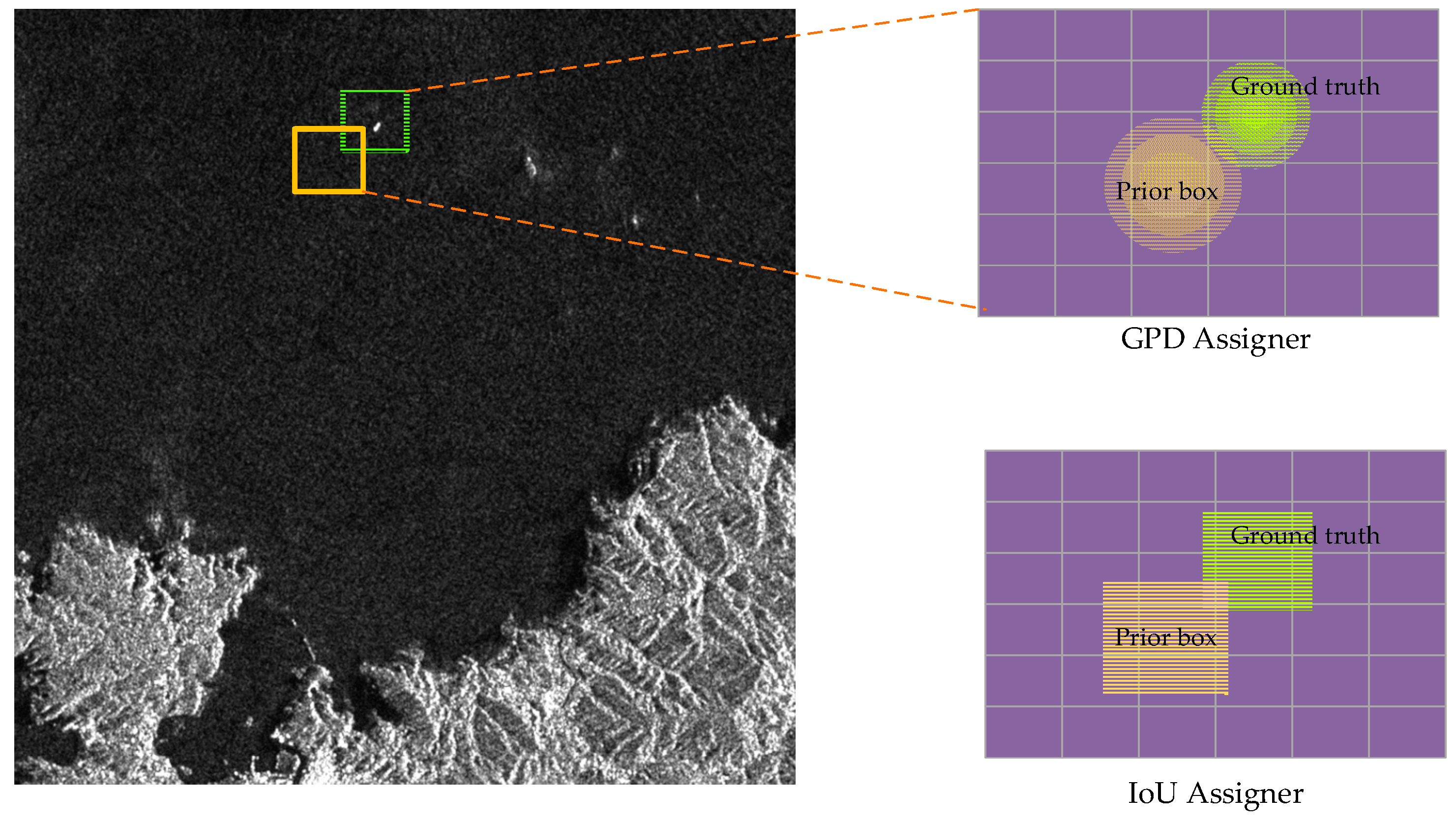
We proposed a Gaussian prior discrepancy (GPD) assigner. This assigner leverages the discrepancy in two Gaussian distributions to judge the matching degree between the prior and ground truth. GPD helps CViTF-Net optimize the discrimination criteria for positive and negative samples.

3.

We designed a level-sync attention mechanism (LSAM). It convolves and fuses multi-layer region of interest (RoI) feature maps, subsequently and adaptively allocating weights to different regions of the feature map. LSAM helps CViTF-Net better utilize low-level features for detecting small ship targets.

2. Materials and Methods

2.1. Method Motivation and Overview

Detecting small ship targets in large-scene SAR images is challenging. The first reason is the low signal-to-noise ratio. As shown in Figure 1a, the inshore part of large-scene SAR images is often affected by noise and clutter interference from land, resulting in poor image quality. Therefore, distinguishing the edges and detailed features of small ship targets is difficult. The second reason is target deformation. As shown in Figure 1b, ships’ movement causes geometric deformation and rotation of their shapes in SAR images, which can cause the blurring or offsetting of the ships’ target positions. These issues could result in missed detections. Finally, there is the issue of data imbalance. In large-scene SAR images, ship targets are typically the minority class in the whole image, with the background occupying the majority. This class imbalance problem may result in the detector’s poor performance when detecting ship targets.

To address the above issues, we propose CViTF-Net, a detector focused on improving the detection performance for small ship targets in large-scale complex-background SAR images. The three innovative parts of this detector are described as follows.

Firstly, we designed a new backbone network consisting of CNNs and visual transformers, called the CViT backbone. CNNs excel at extracting low-level and local features, demonstrating strong perceptual capabilities for details, such as textures. However, in SAR images, small ship targets are often occluded by surrounding noise and clutter, demanding that models possess a robust contextual understanding. Visual transformers, when dealing with sequential data, have the ability to capture global dependencies, which is highly beneficial for target detection in low signal-to-noise ratio environments. The self-attention mechanism of transformers enables networks to consider the global context, while better capturing the relationships between the targets and backgrounds, thus alleviating the challenge of distinguishing targets from backgrounds due to a data imbalance. Therefore, the CViT backbone can simultaneously consider both local and global features, thereby enhancing the accuracy and robustness of small ship target detection.

Secondly, we proposed a GPD assigner, which utilizes two-dimensional Gaussian priors to optimize the discrimination criteria for positive and negative samples. In SAR images, small ship targets may have blurry and offset positions, and noise and clutter may interfere with the target’s position. The center of the two-dimensional Gaussian distribution represents the target’s position, while the variance represents the uncertainty and blurriness of the target’s position. The prior and ground truth boxes are modeled as two-dimensional Gaussian distributions. The discrepancy between these Gaussian distributions measures the similarity between the prior and ground truth. This approach accurately describes the target’s position distribution.

Lastly, we designed an LSAM that simultaneously considers multiple levels in RoI feature maps. Given that low-level features carry more informative details for detecting small ship targets, we first performed convolutional pre-processing on the features from different levels. Then, we fused them into a single feature map. LSAM adaptively assigns different weights to each region within the feature map, allowing for a more precise capturing of details and contextual information on small ship targets. Consequently, even in scenarios marked by a data imbalance, CViTF-Net remains effective in detecting small ship targets.

As shown in Figure 2, CViTF-Net consists of five parts: the CViT backbone, FPN, RPN head, RoI extractor, and RoI head. The CViT backbone relies on fused CNNs and visual transformers to extract features from the input image, outputting four feature maps on different scales, from S1 to S4. The FPN performs feature fusion on the four scales of input feature maps, outputting five new feature maps, from P2 to P6. Three prior boxes with different aspect ratios are generated for each feature point on the five feature maps. The GPD assigner initially converts the priors and ground truths into their corresponding two-dimensional Gaussian distributions, then calculates the discrepancy between these two distributions using the Kullback–Leibler divergence (KLD). This discrepancy can measure the similarity between the ground truth and the prior box, identifying whether a prior box is a positive sample. For each image, the RPN head outputs 1000 region proposals. The RoI uses four feature maps with different scales of output by the FPN, transforming different region size proposals into four groups of 7 × 7 in the RoI feature maps. The LSAM performs convolutional fusion pre-processing on the four RoI feature map groups, assigning weights based on different attention scores within the feature maps. Small ship targets are classified and regressed using two bounding box heads cascaded on the RoI head to enhance detection performance.

2.2. CViT Backbone

In SAR images, small ship targets often confront complex spatial features, such as noise and clutter. The backbone network must process local and global information for feature representation. Therefore, we developed a CViT backbone, as shown in Figure 3. The Meta Conv Block extracts and transforms the input features via grouped convolution and a multi-layer perceptron (MLP). The Meta ViT Block, comprising the multi-head, self-attention and MLP, models the global dependencies and high-level abstract features of the input features.

Inspired by PVTv1 [49], the CViT backbone’s integrated visual transformers maintain a pyramid structure. This structure includes a stem and four stages. Each stage outputs a feature map with the corresponding scale. As shown in Figure 3, the stem consists of four ConvBNReLU layers, where ConvBNReLU combines convolutional operations, batch normalization, and ReLU activation functions. By setting the stride to 2 in the first and fourth ConvBNReLU layers, the resolution of the input image is reduced to one-fourth of its original size, preparing for the subsequent feature extraction stages. Each stage can learn feature representations at different depth levels, with earlier stages focusing more on lower-level visual features, such as edges and textures. As the depth increases, the later stages can learn higher-level abstract features, such as parts of the targets and shapes. This hierarchical feature representation improves the network’s ability to model and discriminate input data, enhancing the performance of small ship target detection in SAR images.

2.2.1. Meta Conv Block

To propose our new design, we first examined recent convolutional block structures. ConvNeXt [50] is a refined convolutional block structure. It bolsters the interaction and integration of features by introducing cross-channel communication in the convolutional layer. However, it remains reliant on local receptive field convolutional operations. ConvNeXt refers to the Swin Transformer architecture for its structure. It includes a series of improvements, such as a macro design and an inverted bottleneck. These enhancements successfully increased the feature extraction power of CNNs, indicating that the convolutional block’s design can gain new insights from visual transformers. Recent studies have shown [51] that the key to the outstanding competitiveness of visual transformers lies in their use of a universal architecture, called the MetaFormer. Therefore, we propose the Meta Conv Block, built upon the MetaFormer structure. This new design employs a convolution block, substituting the transformer’s self-attention mechanism. Moreover, it uses advanced MLP for nonlinear transformation and feature extraction.

As shown in Figure 4a, we referenced ResNeXt [52] and constructed a convolution block using group convolution to alleviate the computational burden and better handle multi-channel feature maps. The definition of group convolution is as follows:

$$Y=Concat\left(Conv2d\left(X_1,W_1\right), Conv2d\left(X_2,W_2\right),\dots ,Conv2d\left(X_i,W_i\right)\right)$$

(1)

$Y$ represents the final concatenated feature map, $Concat$ denotes the operation of concatenating subgroups along the channel dimension, $X_i$ represents the input of the i-th group, and $W_i$ represents the convolution kernel of the i-th group. We used a 3 × 3 convolution kernel to divide the feature map channels into multiple subgroups, with the number of channels set to 32 in each group. Each subgroup was assigned an independent convolution kernel to learn different feature representations. This group convolution helps the detector better capture the relationship between features. As a result, the detector’s nonlinearity, and its receptive field size, increase.

Figure 4. CViT backbone components. (a) Meta Conv Block architecture; (b) MLP architecture; (c) Meta ViT Block architecture.

Figure 4. CViT backbone components. (a) Meta Conv Block architecture; (b) MLP architecture; (c) Meta ViT Block architecture.

After the group convolution, we used a batch normalization layer and ReLU activation function. The batch normalization operation can standardize the feature maps for different channels, thereby improving the stability and trainability of the features. Through the nonlinear transformation of the ReLU activation function, the salient features of the target can be better captured. Consequently, the target’s distinguishability is bolstered. Finally, we applied a 1 × 1 convolution for linear projection, which maintains the same number of channels as the input feature map.

We used multi-layer perceptron (MLP) to introduce nonlinear transformations and feature mappings in neural networks. We used a 1 × 1 convolution to replace the fully connected layer (Figure 4b), handle the spatial structure and channel relationships in the feature maps more effectively, and reduce the number of parameters. Firstly, through a 1 × 1 convolution in the MLP, the channel number of the input feature map is adjusted to the hidden layer’s dimension. To better fit the training data, we set the dimension of the hidden layer to three times the input dimension. This approach ensures the full transmission of the input features’ information to the hidden layer to avoid information loss. Then, we applied an ReLU activation function to the adjusted feature map to perform a nonlinear transformation. The dropout helps prevent overfitting and enhances the model’s robustness. Next, we applied another 1 × 1 convolution, mapping feature maps from the hidden layer dimensions to the output dimensions. This process ensures consistency in the channel numbers between the input and output feature maps.

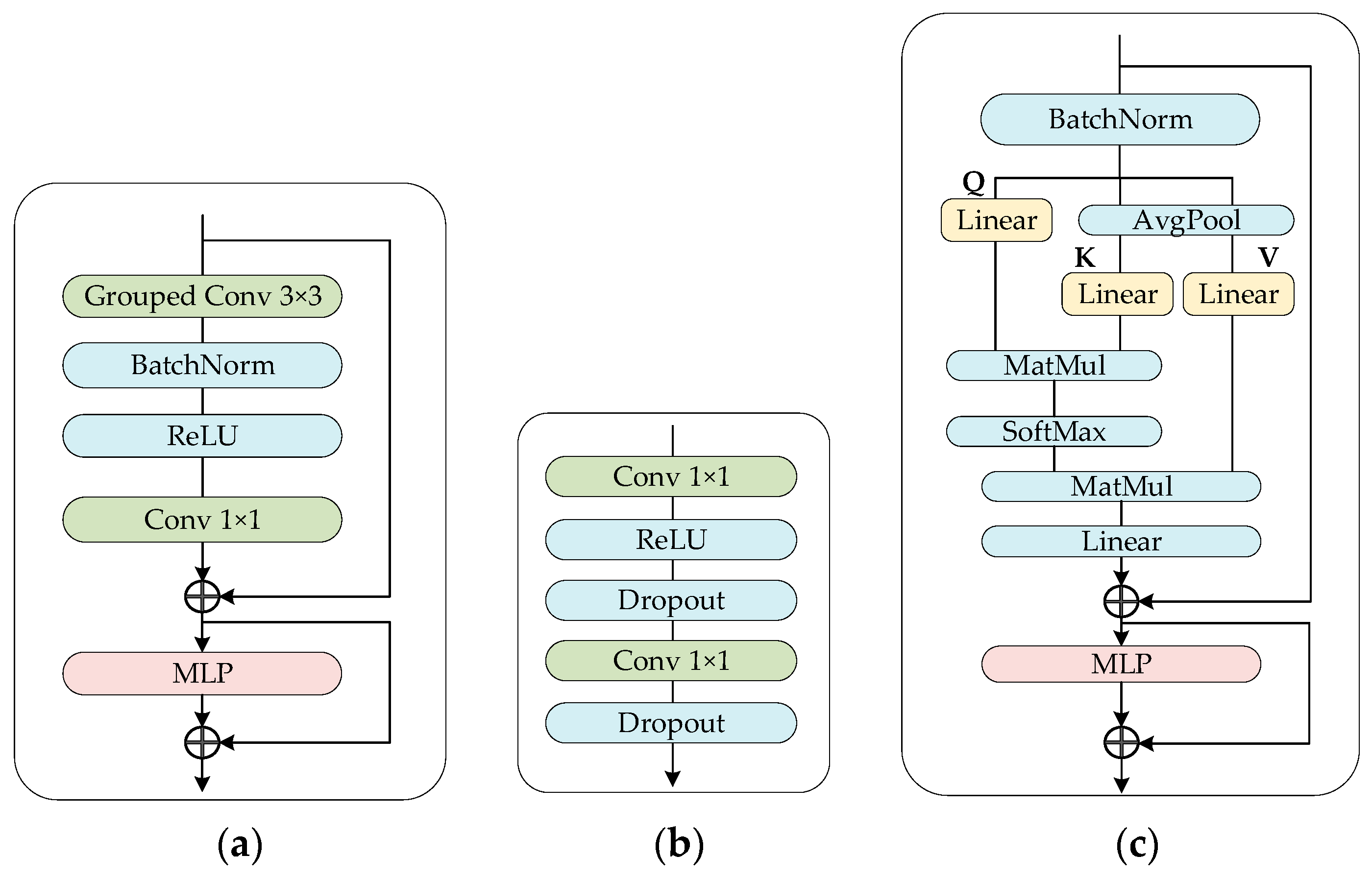
2.2.2. Meta ViT Block

In SAR images, small ship targets are surrounded by noise and clutter. Our aim is to help the detector efficiently capture the complex relationship between the target and background. As depicted in Figure 4c, we used the MetaFormer architecture as the basis of our design. We designed the Meta ViT Block incorporating multi-head, self-attention and MLP.

Firstly, batch normalization is used to normalize the input features, improving the model’s training stability and generalization capabilities. Based on the input dimensions and the set head dimensions of 32 channels, the required number of heads is calculated. Then, the linear transformation layer constructs three learnable weight matrices. These matrices are used to calculate the queries, keys, and values, respectively. Before calculating the keys and values, we first apply average pooling. This pooling operation serves a dual purpose: on the one hand, it reduces computational complexity, while on the other hand, it diminishes the model’s reliance on the input sequence length, enhancing the model’s adaptability to variations in the details of the input image blocks. After downsampling, the input tensor is applied to the linear transformations of the keys and values, respectively. Finally, based on the calculation results for the queries and keys, the self-attention weights are calculated. The attention weights are normalized by Softmax and multiplied by the values to obtain the final self-attention representation. Then, it is mapped to the dimension of the output features through a linear transformation. The multi-head self-attention mechanism is defined by the following formula:

$$MSA\left(X\right)=Concat\left(Hea{d}_1\left(X_1\right),Hea{d}_2\left(X_2\right),\dots ,Hea{d}_i\left(X_i\right)\right)\cdot W^P$$

(2)

where $X$ is the input image block sequence, $Hea{d}_i$ represents the self-attention computation of the i-th head, and $X_i$ is the i-th subset of the input X obtained through a linear transformation. $Concat$ represents concatenating the outputs of multiple attention heads by dimension, and $W^P$ is the weight matrix for projection. In this paper, each self-attention head is defined as follows:

$$Head\left(X\right)=Attention\left(X\cdot W^Q,P_d\left(X\cdot W^K\right),P_d\left(X\cdot W^V\right)\right)$$

(3)

where $X$ represents the input sequence; $W^Q$, $W^K$, and $W^V$ are the weight matrices for the query, key, and value, respectively; and $P_d$ represents input sequence processing through average pooling and downsampling. In addition, the self-attention computation can be represented as follows:

$$Attention\left(Q,K,V\right)=Softmax\left(\frac{Q{K}^T}{\sqrt{d_k}}\right)V$$

(4)

where $Q{K}^T$ represents the product of the query vector and the transpose of the key vector, $V$ represents the value vector, and $d_k$ represents the dimension of the key used to calculate the scaling factor. Finally, through MLP, the Meta ViT Block can extract higher-level feature representations and semantic information.

During processing, multi-head self-attention merges the height and width of the feature maps from the Meta Conv Block into a single dimension and then, after computing the attention, restores this dimension to the pre-merge height and width dimensions, thus preserving the scale of the feature maps. The 1 × 1 convolution in the MLP performs channel-wise linear transformations without altering the width and height of the feature maps, still maintaining the scale of the feature maps. Consequently, within the same stage, the feature map scales in the outputs from both the Meta ViT Block and the Meta Conv Block remain consistent.

2.3. Gaussian Prior Discrepancy (GPD) Assigner

Given the presence of noise and clutter in SAR images, the boundary information for small ship targets may be unclear. Traditional IoU assigners may not accurately match the target’s position. This inaccuracy can decrease detection performance. We propose a GPD assigner to address these issues. This assigner optimizes the similarity measurement between small ship targets’ ground truth and the prior boxes. This method models the ground truth and prior boxes as two-dimensional Gaussian distributions. It uses KLD to measure the similarity between the prior and the ground truth, which describes the position distribution of the target more accurately.

We first generated the prior boxes and used the stride of the five feature maps output from the FPN to generate the corresponding base prior boxes. We began calculating the offset positions of the base prior boxes with respect to the size of the original image. Following this, we added these base prior boxes to the offset positions. In the end, we obtained all the prior boxes from the original image corresponding to the five feature maps.

Algorithm 1 shows the GPD assigner in pseudocode. We first calculated the similarity between all the ground truths and priors. Based on these similarities, we determined whether each prior was a positive sample. To model a two-dimensional Gaussian distribution, we needed the mean vector ${\mu }_e$ and the covariance matrix ${\Sigma }_e$. Therefore, for each ground truth and prior box, we had to calculate its center coordinates, as well as its width and height.

$${\mu }_e=[\begin{array}{c}x\\ y\end{array}],{\Sigma }_e=[\begin{array}{cc}{\sigma }_x^2& 0\\ 0& {\sigma }_y^2\end{array}]$$

(5)

here, $x$ and $y_{}$ are the center coordinates of the prior or ground truth boxes, and ${\sigma }_x^{}$ and ${\sigma }_y^{}$ are half of the box width and height, respectively. Finally, the KLD was used to determine the matching degree between the prior and ground truth. The KLD [53] is a method for measuring the similarity between two probability distributions. In the case of this paper, these two probability distributions are the two-dimensional Gaussian models of the ground truth box and the prior box. The KLD is defined, as follows, in the formula:

$$KL=\left(\frac{w_2^2}{w_1^2}+\frac{h_2^2}{h_1^2}+\frac{4\cdot {(x_1-x_2)}^2}{w_1^2}+\frac{4\cdot {(y_1-y_2)}^2}{h_1^2}+\mathit{log}\left(\frac{w_1^2}{w_2^2}\right)+\mathit{log}\left(\frac{h_1^2}{h_2^2}\right)-2\right)$$

(6)

$$KLD=\frac{1}{1+KL}$$

(7)

where $x_1$, $y_1$ are the center coordinates of the ground truth box; $x_2$, $y_2$ are the center coordinates of the prior box; $w_1^{}$ and $h_1^{}$ are the width and height of the ground truth box, respectively; and $w_2^{}$ and $h_2^{}$ are the width and height of the prior box, respectively. The value of the KLD is between 0 and 1. The closer it is to 1, the more similar the prior box is to the ground truth box. For each prior box, we calculated its maximum KLD value with all the ground truth boxes. If it was <0.8, we set the prior box as a negative sample. Next, for each ground truth box, we set the top three prior boxes related to its maximum KLD as positive samples. The positive and negative samples were used for the subsequent classification and regression target calculations for the RPN.

Algorithm 1. GPD assigner

//Calculate the similarity between a single ground truth and a single prior

function CalculateSimilarity(gt, prior)

x1 ← (gt [0] + gt [2])/2

y1 ← (gt [1] + gt [3])/2

x2 ← (prior [0] + prior [2])/2

y2 ← (prior [1] + prior [3])/2

w1 ← gt [2] − gt [0] + ϵ

h1 ← gt [3] − gt [1] + ϵ

w2 ← prior [2] − prior [0] + ϵ

h2 ← prior [3] − prior [1] + ϵ

kl ← Formula (7)

kld ←Formula (8)

return kld

end function

//Assign a ground truth index to each prior, the default index is 0, representing negative samples.

function AssignGtIndices(gts, priors)

//For each prior, the max kld of all gts, shape (length(priors),)   prior_max_kld ← Call CalculateSimilarity() using gts and priors

assigned_gt_indices ← Create empty array, shape (length(priors),)

neg_inds ← Indices of prior where 0 ≤ prior_max_kld < 0.8   assigned_gt_indices[neg_inds] ← 0   for i ← 1 to length(gts) do     pos_indices ← Indices of top 3 klds related to gts[i] in prior_max_kld     assigned_gt_indices[pos_indices] ← i   end for   return assigned_gt_indices

end function

Figure 5 demonstrates the difference between the GPD assigner and the IoU assigner. In a traditional IoU assigner, if a prior box has a small overlapping area with a ground truth box, its IoU value would be small, even if their centers are very close. Consequently, some prior boxes near the ground truth box but without full overlap could be mislabeled as negative samples. On the contrary, the GPD assigner emphasizes the center position of the box, while considering the shape and size of the box, thus providing a more refined measurement of the similarity between the two boxes. In GPD, two-dimensional Gaussian modeling is employed for prior boxes and ground truth boxes. The center of the two-dimensional Gaussian distribution represents the target’s location, while the variance signifies the uncertainty and fuzziness of the position. This enables us to better represent the potential location range of small ship targets. Moreover, the Gaussian distribution has higher probability density near the target’s location, indicating that our method is more likely to distinguish the targets from background clutter in this area. Therefore, GPD can retain a greater number of effective positive samples.

2.4. Level-Sync Attention Mechanism (LSAM)

Generally, the contrast between the targets and the background in SAR images is low. We proposed the LSAM to help the model effectively capture the subtle feature differences between small ship targets and the background. In the extraction of the RoI feature maps, we used RoI align [54]. Firstly, we mapped the RoI coordinates onto the feature maps output using the FPN. The RoI area is then divided into small regions. Each small region is either upsampled or downsampled to obtain the feature values. Finally, we assembled these into 7 × 7 feature maps with 256 channels.

Algorithm 2 demonstrates the idea of the LSAM in pseudocode. For the input RoI feature maps with different scales, LSAM uses a 5 × 5 convolution kernel in the pre-processing stage to perform the convolution separately, and the output feature maps have the same number of channels as the input. The convolution slides over the input feature map with a stride of 1 and pads 2 pixels around the edges. This setup helps extract richer features and maintains the same size of the output feature maps as the input. Following this, we stacked four layers of RoI feature maps to obtain a comprehensive feature representation containing multi-level abstract information. The above process can be expressed as follows:

$$feat{s}^{\prime }={\displaystyle \sum }_{i=0}^{3}Conv2D\left(feat{s}_i,5,5\right)$$

(8)

where $feat{s}_i$ represents the i-th layer of the feature maps output by RoI align, and $feat{s}^{\prime }$ represents the composite features after stacking.

In the post-processing stage, the input feature map was first mapped to the query, key, and value vectors through a 1 × 1 convolution layer. The query is a feature map with a channel number of 1, while the key and value maintain a channel number of 256. Then, the Softmax function was applied to obtain the attention scores, which indicate the importance of each region, while ensuring that the sum of the scores across all regions is 1. A context vector is calculated by multiplying each region’s key with its corresponding attention score and summing up the products of all the regions. This context vector contains the weighted feature information of all the regions, where the weight of each region is determined by its corresponding attention score.

$$context\_vecto{r}_{}={\displaystyle \sum }_{i=1}^N\left(k_i\cdot attention\_score{s}_i{}_{}\right)$$

(9)

here, $N$ is the number of regions in the feature map, $k_i$ is the key vector of the i-th region, and $attention\_score{s}_i$ is the attention score of the i-th region. Finally, the value is multiplied by the context vector to obtain the weighted feature representation. This representation is then projected back to a channel size of 256 dimensions.

Algorithm 2. Level Sync Attention

function LevelSyncAttention(input_features)   //Preprocessing Stage   conv_features ← Create empty array

for scale ← 1 to length(input_features) do

conv_features[scale] ← Conv2D(input_features[scale],5,5)

end for   combined_features ← Sum of conv_features     //Postprocessing Stage

query, key, value ← Conv2D(combined_features,1,1)

attention_scores ← Softmax(query)

context_vector ← Weighted sum of key and attention_scores

weighted_features ← ReLU(value)·context_vector

output_features ← Conv2D(weighted_features,1,1)

return output_features

end function

Figure 6 describes the architecture of the LSAM. This attention mechanism can automatically adjust the weights of different regions to enhance the target’s visual expression. When processing SAR images with noise, the detector can focus more on the important features of the small ship targets.

3. Results

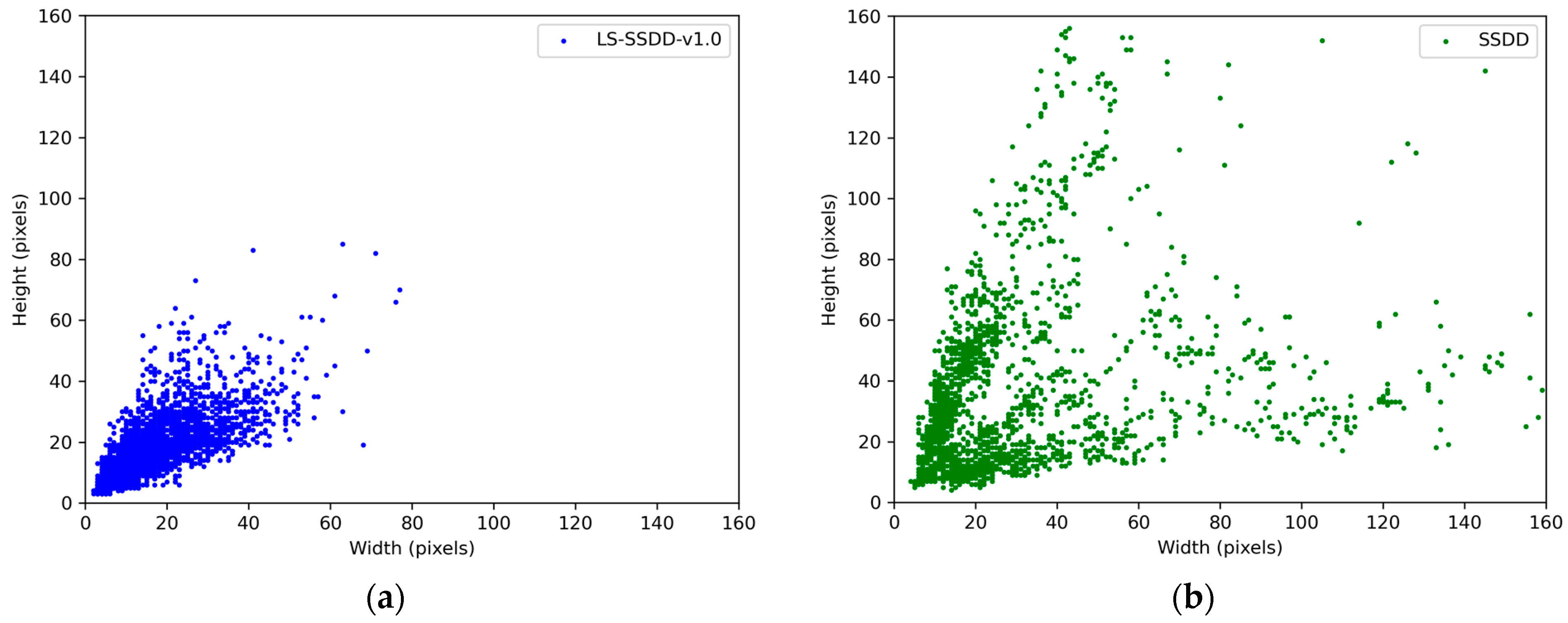
3.1. Introduction of the Datasets

LS-SSDD-v1.0 [55] is an open dataset for detecting small ships from large-scale Sentinel-1 SAR images. It contains 15 large-scale images with dimensions of 24,000 × 16,000 pixels and a swath width of 250 km. We divided these large-scale images into 9000 sub-images, each measuring 800 × 800 pixels, to facilitate network training. In addition, LS-SSDD-v1.0 focuses on small ship detection, with a total of 6015 ships. Among them, 6003 are small ships, accounting for 99.80% of the total. LS-SSDD-v1.0 uses VV polarization to annotate ship locations. It contains pure background images that do not include annotated ships. The backgrounds incorporated encompass a variety of elements, such as the pure sea surface, urban areas, rivers, land, islands, and ports. The coastline of the imaged area in the dataset is complex, with the area of land being smaller than that of the sea. Ships are densely distributed in rivers.

The SAR ship detection dataset (SSDD) is the first open dataset in the field of SAR image ship detection based on deep learning. We use the official version of the SSDD [56]. Unlike LS-SSDD-v1.0, the image resolution in the SSDD is not fixed, with widths ranging from 214 to 668 pixels, and heights from 160 to 526 pixels. The median size of the images is 500 × 333 pixels. Following the original paper setting, 232 images with the last digit of the file number being 1 and 9 are uniquely determined as the test set, while the remaining 928 images are considered the training set. Ships in the SSDD have rich diversity, including densely distributed small targets and ships docked in parallel in ports.

Table 1. Dataset information.

Parameter	LS-SSDD-v1.0	SSDD
Satellite	Sentinel-1	RadarSat-2, TerraSAR-X, Sentinel-1
Image size (pixel)	800 × 800	500 × 333
Image number	9000	1160
Train/test ratio	6000/3000	928/232
Ship number	6015	2456
Avg. ship size (pixel2)	381	1882
Scenes	Inshore and offshore	Inshore and offshore

describes basic information about the two datasets, including the satellite source, image size, number of images, etc. The size of the SAR images in LS-SSDD-v1.0 is larger, and the size of the ship targets is smaller. Figure 7 reflects the distribution of the width and height pixel values for the ship targets’ ground truth in the two datasets. The width and height of most ship targets in the LS-SSDD-v1.0 are smaller, while the size of the ship targets in the SSDD varies more.

3.2. Evaluation Criterions

In line with the evaluation criteria in the original paper for LS-SSDD-v1.0, we used the precision, recall, F1 score, and mean average precision (mAP). The precision and recall help determine the model classification accuracy and missed detection situations. The F1 synthesizes information from both, and the mAP assesses the balance between the accuracy and recall of the object detection model. These indicators provide a comprehensive evaluation of model performance.

Precision, also known as the positive predictive value, represents the proportion of targets identified as ships by the model that are actually ships. True positives (TPs) refers to the number of targets correctly identified as ships by the model. False positives (FPs) refer to the number of targets incorrectly identified as ships by the model (which are not actually ships). Precision is calculated as follows:

$$Precision=\frac{TP}{TP+FP}$$

(10)

Recall, also known as sensitivity, represents the proportion of all the actual ship targets that are successfully identified by the model. TPs are as previously described, and false negatives (FNs) are the number of targets incorrectly identified as non-ships by the model (which are actually ships). Recall is calculated as follows:

$$Recall=\frac{TP}{TP+FN}$$

(11)

The F1 score is the harmonic mean of the precision and recall that can be used as a measurement standard for both the precision and recall.

$$F1=2\times \frac{Precision\cdot Recall}{Precision+Recall}$$

(12)

The mAP is a measure of the model’s precision at different recall. It can reflect the stability of the model’s precision when the recall varies, as well as the model’s overall performance.

$$mAP={{\displaystyle \int }}_0^{1}P\left(R\right)\cdot dR$$

(13)

P(R) represents the precision at a given recall.

3.3. Implementation Details

Table 2. Experimental environment.

Configuration	Parameter
CPU	AMD EPYC 7543 32-Core Processor
GPU	NVIDIA RTX A5000 ×4
Operating system	Ubuntu 20.04.4 LTS
Development tools	Python 3.10.8, Pytorch 1.13.0+cu117

describes the experimental environment described in this paper.

Our experiments were based on MMDetection [57], and the number of training epochs for both the LS-SSDD-v1.0 and SSDD datasets was 12. The original dataset settings were adopted for the training set, test set, inshore test set, and offshore test set. We used an AdamW optimizer, with an initial learning rate of 0.0001. The weight decay of the optimizer was 0.05, and the learning rate was dynamically adjusted using cosine annealing with learning rate restarts. The learning rate restart cycle was 6 epochs, and the minimum learning rate was 5 × 10⁻⁶. The batch size was set to 16, with four samples per GPU for four GPUs. During the testing phase, the image size was set to 1000 × 1000, and the score threshold was set to 0.5. We conducted three separate runs of the experiments and calculated the averages of the obtained results to ensure the stability and reliability of the experimental outcomes.

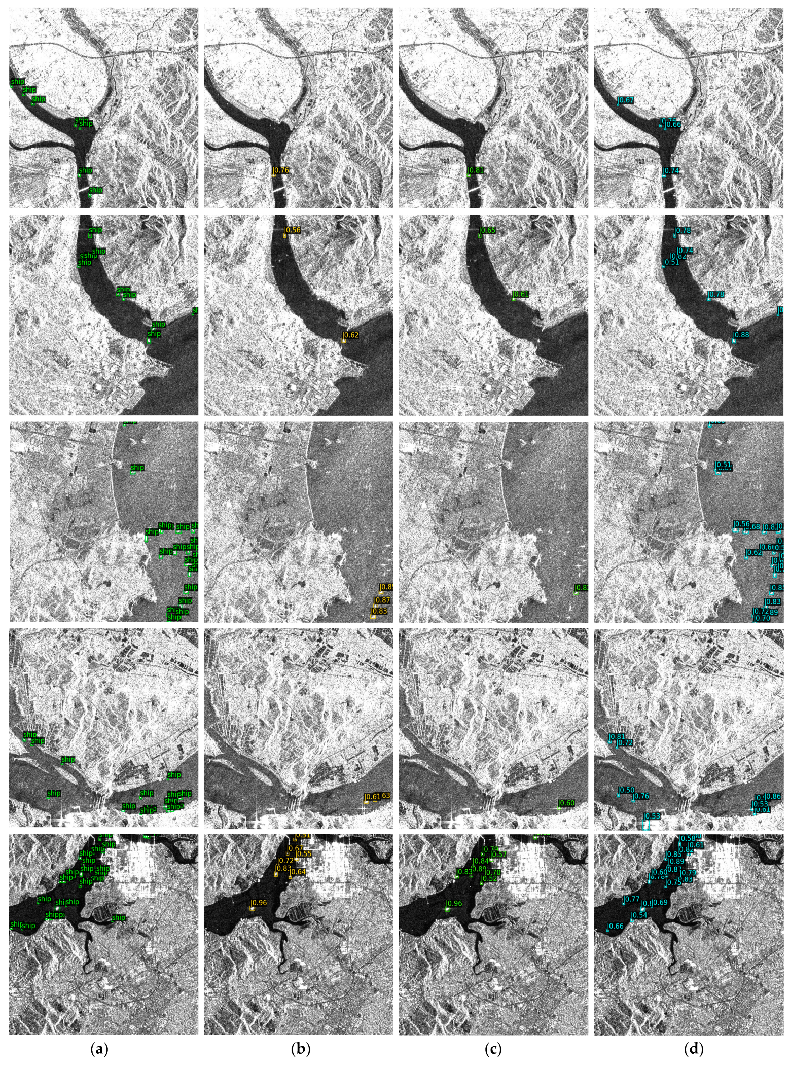
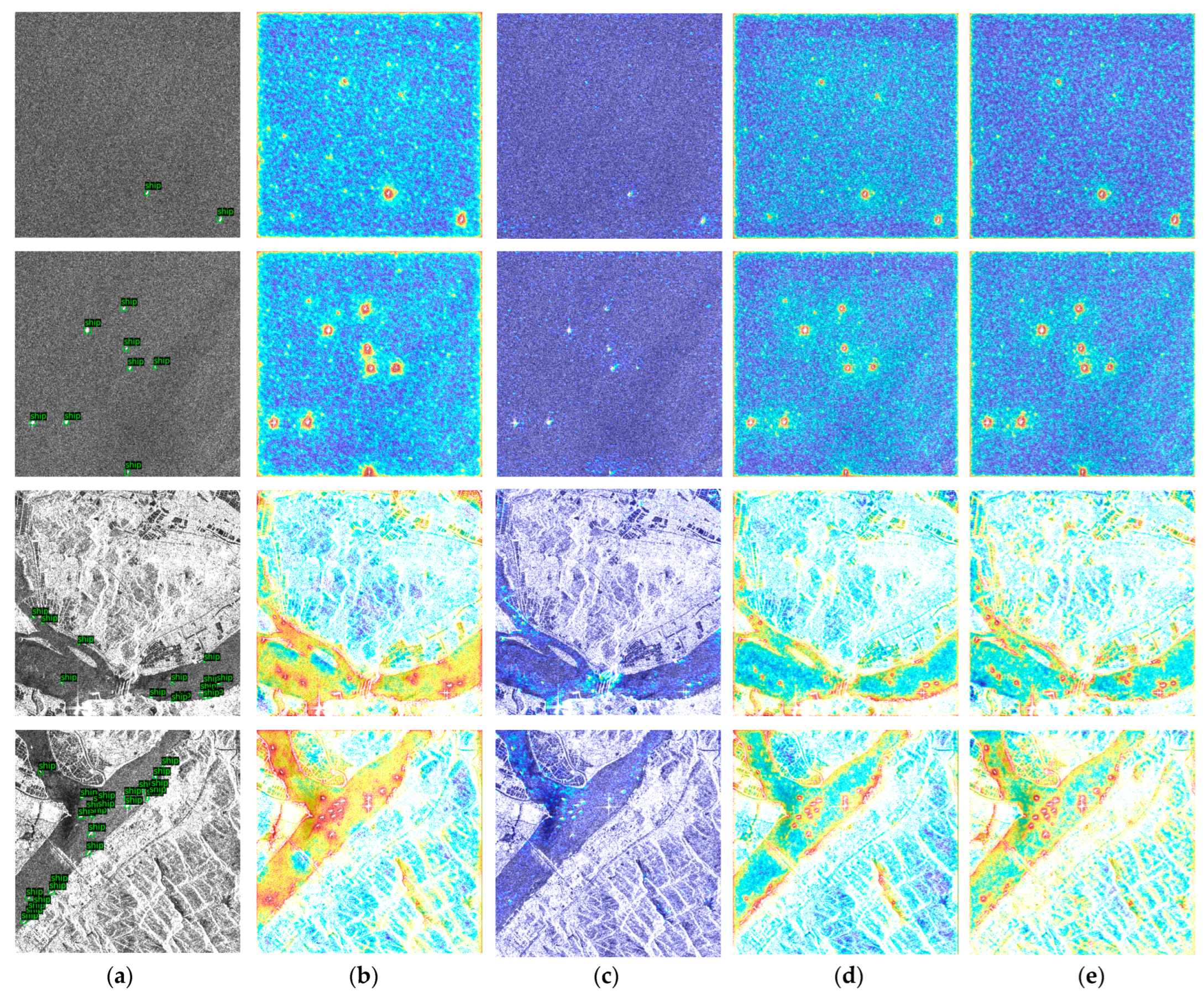
3.4. Results for LS-SSDD-v1.0

As depicted in

Table 3. Results for the entire LS-SSDD-v1.0 scene.

Method	Precision	Recall	mAP	F1
FPN [12]	0.805	0.706	0.680	0.752
Cascade R-CNN [15]	0.822	0.700	0.694	0.756
Libra R-CNN [20]	0.821	0.690	0.678	0.749
Double Head R-CNN [58]	0.815	0.704	0.685	0.755
DCN [59]	0.766	0.730	0.700	0.747
YOLOX-L [30]	0.687	0.732	0.698	0.708
YOLOv7-X [60]	0.690	0.728	0.686	0.708
HR-SDNet [61]	0.849	0.705	0.688	0.770
MHASD [62]	0.834	0.679	0.755	0.748
SII-Net [16]	0.682	0.793	0.761	0.733
A-BFPN [19]	0.850	0.736	0.766	0.788
CMA-SSJC [63]	0.704	0.803	0.772	0.750
CViTF-Net	0.784	0.834	0.797	0.808

, we conducted detailed experiments on the LS-SSDD-v1.0 dataset to validate CViTF-Net’s performance in detecting small ship targets in large-scale complex-background SAR images.

In Table 3, we present the comparative results against existing state-of-the-art SAR ship detectors for the entire test dataset. The first seven rows represent general object detection methods, while rows 8 to 13 (from HR-SDNet to CMA-SSJC) display results from other researchers on the LS-SSDD-v1.0 dataset. The final row, CViTF-Net, represents our proposed approach. YOLOX and YOLOv7 are single-stage object detectors. In this study, we employed YOLOX-L and YOLOv7-X models, using larger model architectures and more parameters to enhance detection performance. From Table 3, it can be observed that HR-SDNet excels on precision with a high score of 0.849, effectively reducing false positives. The F1 score is also relatively high, but it suffers from a lower recall rate, indicating the presence of more false negatives, and a relatively lower mAP. MHASD boasts high precision at 0.834, but a recall rate of only 0.679, indicating more missed detections, thus limiting the mAP and F1 scores. SII-Net excels on the recall rate and achieves a relatively high mAP of 0.761, but it has a lower precision at 0.682, suggesting more false positives. A-BFPN’s strength lies in the highest precision at 0.850, but with an average recall rate. CMA-SSJC achieves a recall rate of 0.803, a relatively high mAP, but a lower precision of 0.704, indicating more false positives. Compared to other research, our proposed CViTF-Net demonstrates outstanding performance on the recall rate, mAP, and F1 scores, reaching the highest levels. However, some other models have a certain advantage in the precision metric, such as HR-SDNet and A-BFPN, both showing strong precision performance. The results for LS-SSDD-v1.0 further establish the superiority of CViTF-Net in detecting small ship targets in large-scale complex-background SAR images.

Table 4. The inshore scene results for LS-SSDD-v1.0.

Method	Precision	Recall	mAP	F1
FPN [12]	0.698	0.376	0.341	0.488
Cascade R-CNN [15]	0.739	0.369	0.358	0.492
Libra R-CNN [20]	0.734	0.342	0.313	0.466
Double Head R-CNN [58]	0.743	0.373	0.338	0.496
DCN [59]	0.683	0.408	0.364	0.510
YOLOX-L [30]	0.686	0.431	0.392	0.529
YOLOv7-X [60]	0.504	0.414	0.327	0.454
HR-SDNet [61]	0.760	0.378	0.348	0.504
MHASD [62]	0.576	0.422	0.438	0.487
SII-Net [16]	0.461	0.554	0.469	0.503
A-BFPN [19]	0.770	0.545	0.471	0.638
CMA-SSJC [63]	0.502	0.586	0.522	0.540
CViTF-Net	0.643	0.656	0.579	0.649

and

Table 5. The results on the offshore scene for LS-SSDD-v1.0.

Method	Precision	Recall	mAP	F1
FPN [12]	0.836	0.901	0.876	0.867
Cascade R-CNN [15]	0.845	0.895	0.889	0.869
Libra R-CNN [20]	0.843	0.897	0.869	0.869
Double Head R-CNN [58]	0.835	0.899	0.870	0.865
DCN [59]	0.792	0.920	0.892	0.851
YOLOX-L [30]	0.687	0.909	0.877	0.782
YOLOv7-X [60]	0.766	0.913	0.882	0.833
HR-SDNet [61]	0.875	0.899	0.883	0.886
MHASD [62]	0.905	0.857	0.915	0.880
SII-Net [16]	0.819	0.934	0.916	0.872
A-BFPN [19]	0.921	0.889	0.921	0.904
CMA-SSJC [63]	0.827	0.931	0.909	0.875
CViTF-Net	0.875	0.939	0.923	0.905

list the results for inshore and offshore scenes in the LS-SSDD-v1.0 test set. Large-scale SAR images often include inshore scenes with complex background interference. In these scenes, ships typically exhibit smaller sizes and low contrast. This complexity generally results in lower ship detection performance in inshore areas. In Table 4, CViTF-Net is the best-performing detector with an mAP of 0.579 and an F1 of 0.649, indicating that it can more effectively cope with inshore scene challenges, such as complex backgrounds, noise interference, and small target sizes. Table 5 shows that CViTF-Net also demonstrates the best performance on offshore scenes. However, the gap with A-BFPN is not significant. Compared to inshore scenes, offshore scenes usually have a simpler background. Simple backgrounds allow the detectors to focus more easily on ship target areas.

Figure 8 presents the visualization results for the inshore scenes in the LS-SSDD-v1.0 test set. Figure 8a represents the ground truths, and Figure 8b shows the Double Head RCNN results. Figure 8c displays the YOLOX-L results, and Figure 8d displays the CViTF-Net results. Inshore areas usually contain a large amount of complex background interference, including terrain, buildings, vegetation, etc. These interferences may have similar textures, shapes, and sizes to the ship targets, making it difficult to distinguish the ships from the background. Additionally, noise and speckles may create variations in image brightness, further blurring target edges and details. Compared to Double Head RCNN and YOLOX-L, CViTF-Net’s detection results still exhibit cases of missed detections and false alarms, but are closer to the ground truth. It can identify more small ship targets on complex backgrounds, indicating that CViTF-Net effectively enhances inshore scene detection performance. Our method is specialized for the task of detecting small ship targets in large-scale complex-background SAR images, and the model leans towards minimizing false negatives by emphasizing the detection of more targets, even if it results in lower confidence scores for certain smaller or atypical targets.

3.5. Results on SSDD

As shown in

Table 6. The results for the entire SSDD scene.

Method	Precision	Recall	mAP	F1
FPN [12]	0.884	0.941	0.936	0.911
Cascade R-CNN [15]	0.914	0.939	0.934	0.926
Libra R-CNN [20]	0.861	0.946	0.939	0.901
Double Head R-CNN [58]	0.905	0.945	0.942	0.924
DCN [59]	0.931	0.952	0.950	0.941
YOLOX-L [30]	0.797	0.965	0.950	0.872
YOLOv7-X [60]	0.843	0.917	0.899	0.878
HR-SDNet [61]	0.964	0.909	0.908	0.935
SER Faster R-CNN [64]	0.861	0.922	0.915	0.890
Quad-FPN [65]	0.895	0.957	0.952	0.924
RIF [66]	0.946	0.932	0.962	0.938
SII-Net [16]	0.861	0.968	0.955	0.911
A-BFPN [19]	0.975	0.944	0.968	0.959
CViTF-Net	0.943	0.981	0.978	0.961

, we conducted comparative experiments on the SSDD dataset to explore the detector’s stability and generality, and provide a more comprehensive performance evaluation. The first seven rows represent general object detection methods, while rows 8 to 13 (from HR-SDNet to A-BFPN) display results from other researchers on the SSDD dataset. The final row, CViTF-Net, represents our proposed approach. HR-SDNet excels on precision (precision) with a score of 0.964, indicating a reduction in false positives during detection. However, it falls short on the recall rate (recall), suggesting limitations in its performance for small target detection. SER Faster R-CNN exhibits slightly lower precision and average recall. Quad-FPN shines on the recall rate, achieving a score of 0.957, indicating its ability to capture targets effectively, but it has relatively lower precision, potentially leading to more false positives. RIF performs exceptionally well on the mAP (mean average precision), reaching 0.962, indicating strong overall performance. SII-Net achieves a very high recall rate of 0.968, signifying high performance on target capture, but it has relatively lower precision, potentially experiencing some false positive issues. A-BFPN demonstrates high precision and mAP, indicating a strong overall performance. In contrast, our CViTF-Net excels on the recall rate, mAP, and F1 metrics, reaching 0.981, 0.978, and 0.961, respectively. This indicates that it can maintain high accuracy, while ensuring comprehensive target detection. It also demonstrates the robustness and adaptability of CViTF-Net, showcasing its potential in the field of ship target detection. Although the design of the CViTF-Net structure did not yield the highest precision, our model shows competitive advantages on its overall performance compared to other models.

Following the SSDD test set configuration, we also conducted experiments on inshore and offshore scenes.

Table 7. The results for the inshore SSDD scene.

Method	Precision	Recall	mAP	F1
FPN [12]	0.741	0.848	0.823	0.790
Cascade R-CNN [15]	0.786	0.837	0.810	0.810
Libra R-CNN [20]	0.686	0.854	0.817	0.760
Double Head R-CNN [58]	0.769	0.854	0.838	0.809
DCN [59]	0.862	0.877	0.869	0.869
YOLOX-L [30]	0.626	0.924	0.874	0.746
YOLOv7-X [60]	0.655	0.808	0.748	0.723
HR-SDNet [61]	0.907	0.744	0.736	0.817
SER Faster R-CNN [64]	0.663	0.790	0.745	0.720
Quad-FPN [65]	0.747	0.877	0.846	0.806
RIF [66]	0.903	0.762	0.852	0.826
A-BFPN [19]	0.935	0.756	0.883	0.836
CViTF-Net	0.883	0.965	0.958	0.922

shows the results for ship target detection in the inshore scenes. CViTF-Net achieved the best comprehensive evaluation results for the inshore scenes.

Table 8. The results for the SSDD offshore scene.

Method	Precision	Recall	mAP	F1
FPN [12]	0.958	0.984	0.982	0.970
Cascade R-CNN [15]	0.976	0.986	0.985	0.980
Libra R-CNN [20]	0.958	0.989	0.988	0.973
Double Head R-CNN [58]	0.973	0.986	0.986	0.979
DCN [59]	0.963	0.986	0.985	0.974
YOLOX-L [30]	0.904	0.984	0.977	0.942
YOLOv7-X [60]	0.940	0.967	0.961	0.953
HR-SDNet [61]	0.986	0.986	0.985	0.986
SER Faster R-CNN [64]	0.968	0.983	0.982	0.975
Quad-FPN [65]	0.973	0.994	0.993	0.983
RIF [66]	0.985	0.982	0.992	0.983
A-BFPN [19]	0.989	0.987	0.995	0.987
CViTF-Net	0.983	0.994	0.993	0.988

presents the offshore scene results. The offshore scenes in the SSDD dataset are characterized by simple backgrounds, larger target sizes, and higher contrasts, facilitating ship target detection. Therefore, CViTF-Net’s performance is comparable to current methods. The mAP and F1 for CViTF-Net for both the inshore and offshore scenes further verify its accuracy and comprehensive performance in ship target detection.

Figure 9 shows the visualization results for the inshore scenes for the SSDD dataset. Figure 9a represents the ground truth of the ships, Figure 9b represents the Double Head R-CNN results, Figure 9c represents the DCN results, Figure 9d represents the YOLOX-L results, and Figure 9e represents our CViTF-Net results. By comparing the results with actual ships, we have marked false positive cases with red circles. Based on our observations, we found that humans can easily distinguish non-ship targets on land and at sea. However, identifying targets along the shoreline can also be challenging for humans. According to the visualization results, CViTF-Net’s detection results are close to the ground truth, with accurate bounding boxes and corresponding high confidence scores, indicating that it can accurately identify and locate ship targets in complex scenes from the SSDD dataset. In the last scenario, CViTF-Net successfully avoided mistaking large port facilities for ships. The LSAM allows CViTF-Net to effectively process feature information at different scales, thereby enhancing its detection ability for multi-scale ship targets.

In observing the experimental results for the LS-SSDD-v1.0 and SSDD datasets, CViTF-Net exhibits a precision value that may not be the highest; however, it attains superior levels in terms of the recall, mAP, and F1. The underlying rationales for this phenomenon can be delineated as follows:

1.

Design of CViTF-Net: The architecture of CViTF-Net is configured such that the global feature information extracted by the CViT backbone aids the model in effectively managing background interference, consequently elevating the true positive rate for object detection, thereby augmenting recall. The GPD assigner leverages a two-dimensional Gaussian distribution centered on the target’s position, with the variance representing the uncertainty in the target’s location. This approach allows for more accurate matching of targets to prior boxes, even in cases of slight positional offsets or blurriness, thereby reducing the false negative rate and enhancing recall. The LSAM component excels in capturing intricate target details and contextual information, further reducing the false negative rate and enhancing recall.

2.

Precision–recall trade-off: Typically, when a model endeavors to increase recall (i.e., reduce false negatives), it may inadvertently classify some non-target regions as targets, leading to a decrease in precision (an increase in false positives). This phenomenon represents a common trade-off.

3.

Comprehensive evaluation with F1 and mAP: The F1 score takes both precision and recall into account simultaneously, while mAP provides a comprehensive assessment of the model’s performance at various thresholds. Consequently, even though CViTF-Net may exhibit relatively lower precision, its overall performance remains outstanding.

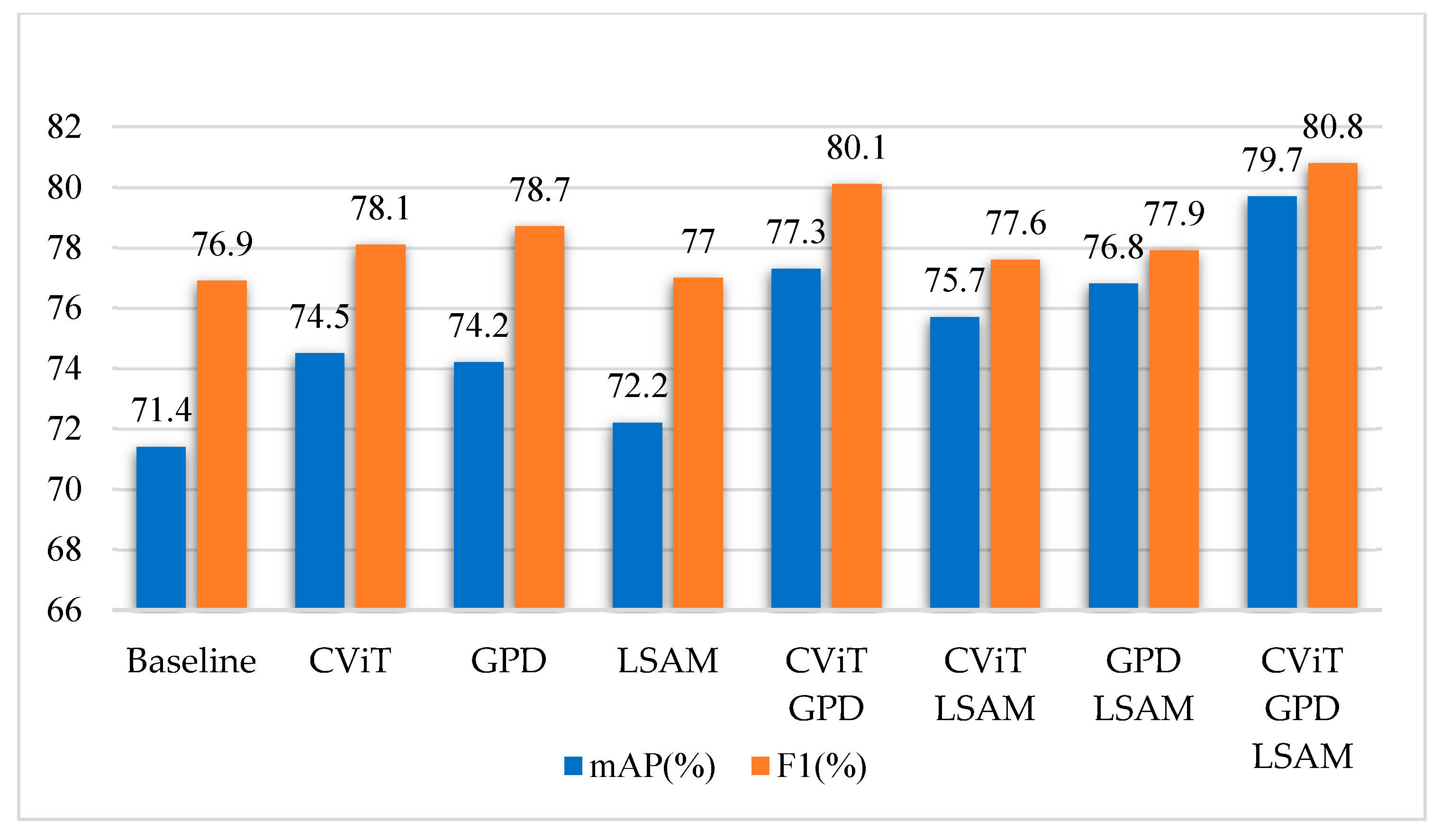
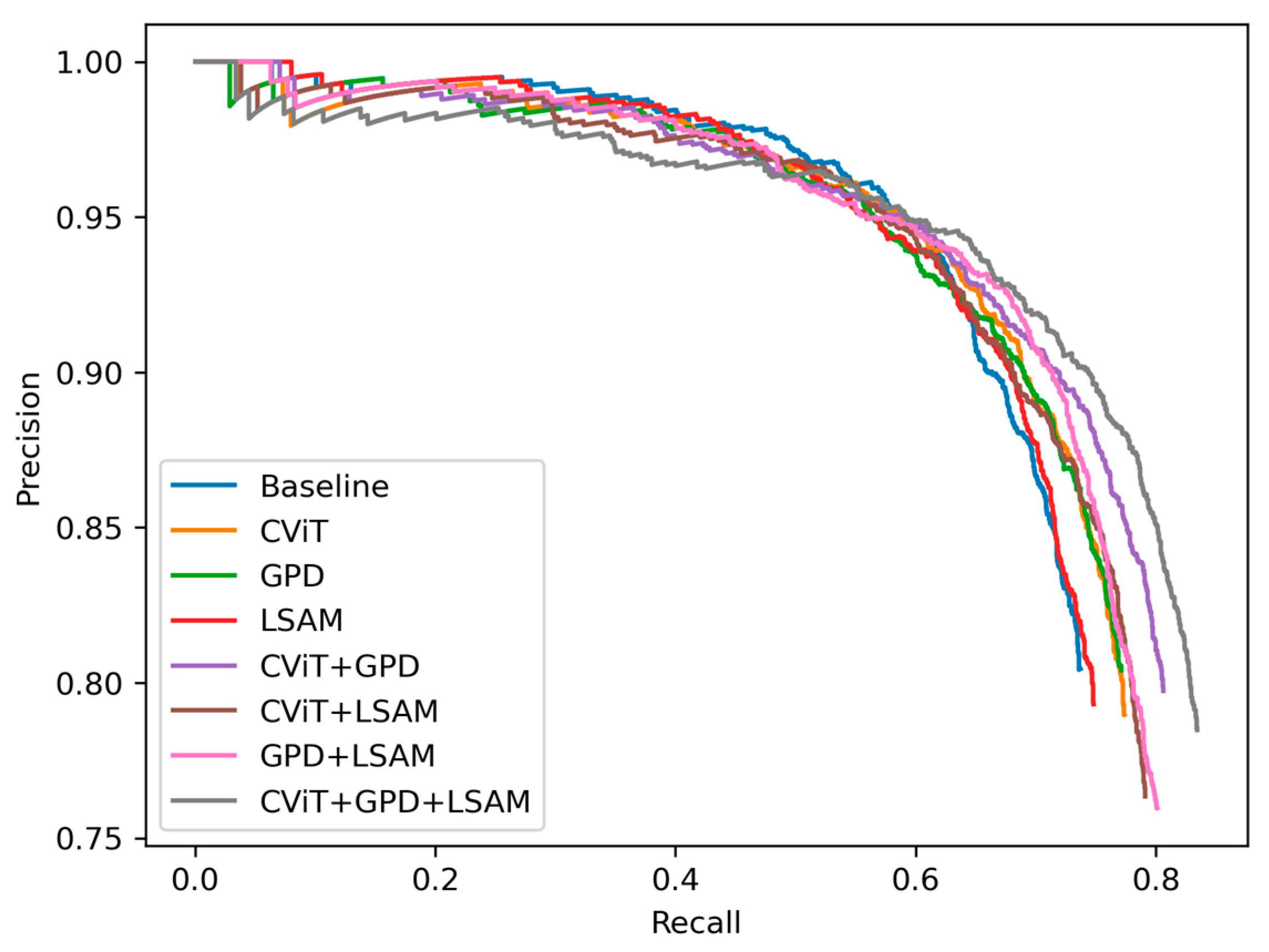
4. Ablation Experiment

To understand the specific contributions from the three innovative components in CViTF-Net, as shown in

Table 9. The results for different components for the entire LS-SSDD-v1.0 scene.

CViT	GPD	LSAM	Precision	Recall	mAP	F1	GFLOPs	Params(M)
-	-	-	0.804	0.737	0.714	0.769	171.94	79.62
√	-	-	0.789	0.773	0.745	0.780	205.74	90.97
-	√	-	0.802	0.771	0.742	0.786	171.94	79.62
-	-	√	0.793	0.748	0.722	0.769	191.76	83.3
√	√	-	0.797	0.806	0.773	0.801	205.74	90.97
√	-	√	0.763	0.791	0.757	0.776	225.56	94.65
-	√	√	0.759	0.801	0.768	0.779	191.76	83.3
√	√	√	0.784	0.834	0.797	0.808	225.56	94.65

, we conducted an ablation study on the entire test set of LS-SSDD-v1.0. Figure 10 shows a bar chart on the mAP and F1 in the ablation study, describing the detectors’ comprehensive performance when different components are combined. From the ablation experiment results, we can see that when using the CViT backbone, GPD assigner, and LSAM simultaneously, the mAP and F1 are 0.797 and 0.808, respectively. This performance is better than using any single component or combination of two components, indicating that CViTF-Net, as a whole, is effective.

The analysis for each individual component is as follows:

1.

CViT backbone (CViT): The detector’s recall, mAP, and F1 improved when only the CViT was enabled compared to not enabling any components, especially the recall and mAP, which increased by 3.6% and 3.1%, respectively. However, a slight decrease was observed in the precision, which can be attributed to CViT’s proficiency in capturing global information, possibly at the expense of some detail features. Despite this, the CViT significantly improves the overall performance of the detector.

2.

GPD assigner (GPD): When only the GPD was enabled, compared to not enabling any components, the detector’s recall increased by 3.4%, the mAP increased by 2.8%, and the F1 increased by 1.8%, while maintaining the same precision. Meanwhile, compared to enabling the CViT and LSAM, but not the GPD, the precision rose from 0.763 to 0.802. This finding indicates that the GPD’s utilization of the two-dimensional Gaussian prior notably optimizes the sample discrimination criteria. It plays a crucial role in boosting the performance of the detector. Since the GPD assigner is an optimization strategy for allocating positive and negative samples and does not involve changes to the model architecture, the model’s GFLOPs and Params(M) are not affected by the GPD.

3.

LSAM: When only the LSAM was enabled, and not the CViT or GPD, compared to not enabling any components, the impact on the precision was slightly insufficient. The recall and mAP improved, but the F1 remained essentially unchanged. This finding suggests that the LSAM played a positive role in processing the RoI feature maps, helping the detector reduce the missed detection rate.

Figure 11 presents the PR curve for the ablation study. Overall, each component contributes to the performance improvement of the detector. CViTF-Net achieves the largest area under the curve and the best overall performance when all the components are enabled. This highlights the importance of the collaborative work of the CViT, GPD, and LSAM. Additionally, it validates the rationality and effectiveness of CViTF-Net’s design.

We created a feature map visualization experiment to understand the degree of attention each component in CViTF-Net pays to the different areas in the SAR images, as shown in Figure 12. Here, the colors range from deep blue to bright red, indicating attention levels from low to high. Figure 12a shows the ground truth, illustrating the actual positions of the small ship targets. Figure 12b displays the scenario without any enabled components, serving as a baseline (Cascade R-CNN) for comparison with the three innovative components proposed in our approach. The baseline detector is clearly influenced by noise, manifesting a tendency towards false alarms. Figure 12c demonstrates a situation when only the CViT backbone is activated. At this point, the detector demonstrates a stronger capability for global feature representation. In addition, the region of interest becomes more concentrated on small ship targets, while attention to the background significantly decreases. Figure 12d depicts a scenario where only the GPD assigner is employed. In this case, the detector pays more accurate attention to the location of the small ship targets. It refines the discrimination criteria for positive and negative samples using the two-dimensional Gaussian prior. Consequently, the detector emphasizes regions near the target center more during training. Figure 12e illustrates a case where only the LSAM is enabled. Due to the LSAM’s ability to better capture the details and context information about the target, observing the third and fourth rows in Figure 12, it can be observed that the detector’s perception range of the target is more refined, with a certain noise suppression effect when compared to the baseline (Figure 12b).

5. Conclusions

To address the challenge of detecting small ship targets in large-scale complex-background SAR images, we propose a new two-stage detector, CViTF-Net, which integrates CNNs and visual transformers in a novel manner. CViTF-Net includes three innovative components: a CViT backbone, Gaussian prior discrepancy (GPD) assigner, and level-sync attention mechanism (LSAM). By integrating local and global information, optimizing the sample discrimination criteria using two-dimensional Gaussian priors, and adaptively enhancing the feature representation of the RoI feature maps with the LSAM, CViTF-Net effectively improves the accuracy and robustness of small ship target detection.

Firstly, we conducted comparative experiments with CViTF-Net and the current advanced SAR ship detectors using the LS-SSDD-v1.0 dataset, which is specifically designed for small ship targets. Our experimental results indicated that CViTF-Net achieved the best performance for both the mAP and F1. The SAR image detection visualization shows that it closely aligns with the ground truth and that it significantly improves the detection performance for ships in complex inshore scenes. The experimental results on the SSDD dataset demonstrate the robustness and versatility of CViTF-Net.

Moreover, we also conducted ablation experiments and feature map visualization experiments to verify the effectiveness and rationality of our method. Our ablation studies indicate that all three innovative components of CViTF-Net contribute to the overall enhancement of detection performance. Using our method, visualization of the feature map shows that the detector can more accurately focus on the locations of small ship targets, while suppressing background noise.

We will explore the use of oriented bounding boxes to accurately describe ships’ shapes and directions in future research. We will investigate how to improve self-attention mechanisms or introduce new visual transformer structures to enhance the detection accuracy for small ship targets.

References

1. Wang, Y.; Yang, W.; Chen, J.; Kuang, H.; Liu, W.; Li, C. Azimuth Sidelobes Suppression Using Multi-Azimuth Angle Synthetic Aperture Radar Images. Sensors 2019, 19, 2764. [Google Scholar] [CrossRef] [PubMed]
2. Chang, W.; Tao, H.; Sun, G.; Wang, Y.; Bao, Z. A Novel Multi-Angle SAR Imaging System and Method Based on an Ultrahigh Speed Platform. Sensors 2019, 19, 1701. [Google Scholar] [CrossRef] [PubMed]
3. Sonkar, A.; Kumar, S.; Kumar, N. Spaceborne SAR-Based Detection of Ships in Suez Gulf to Analyze the Maritime Traffic Jam Caused Due to the Blockage of Egypt’s Suez Canal. Sustainability 2023, 15, 9706. [Google Scholar] [CrossRef]
4. Malyszko, M. Fuzzy Logic in Selection of Maritime Search and Rescue Units. Appl. Sci. 2022, 12, 21. [Google Scholar] [CrossRef]
5. Bai, L.; Yao, C.; Ye, Z.; Xue, D.; Lin, X.; Hui, M. Feature Enhancement Pyramid and Shallow Feature Reconstruction Network for SAR Ship Detection. IEEE J. Sel. Top. Appl. Earth Obs. Remote Sens. 2023, 16, 1042–1056. [Google Scholar] [CrossRef]
6. Chen, S.; Li, X. A New CFAR Algorithm Based on Variable Window for Ship Target Detection in SAR Images. Signal Image Video Process. 2019, 13, 779–786. [Google Scholar] [CrossRef]
7. Ai, J.; Mao, Y.; Luo, Q.; Xing, M.; Jiang, K.; Jia, L.; Yang, X. Robust CFAR Ship Detector Based on Bilateral-Trimmed-Statistics of Complex Ocean Scenes in SAR Imagery: A Closed-Form Solution. IEEE Trans. Aerosp. Electron. Syst. 2021, 57, 1872–1890. [Google Scholar] [CrossRef]
8. Liu, T.; Yang, Z.; Yang, J.; Gao, G. CFAR Ship Detection Methods Using Compact Polarimetric SAR in a K-Wishart Distribution. IEEE J. Sel. Top. Appl. Earth Obs. Remote Sens. 2019, 12, 3737–3745. [Google Scholar] [CrossRef]
9. Li, N.; Pan, X.; Yang, L.; Huang, Z.; Wu, Z.; Zheng, G. Adaptive CFAR Method for SAR Ship Detection Using Intensity and Texture Feature Fusion Attention Contrast Mechanism. Sensors 2022, 22, 8116. [Google Scholar] [CrossRef]
10. Yasir, M.; Jianhua, W.; Mingming, X.; Hui, S.; Zhe, Z.; Shanwei, L.; Colak, A.T.I.; Hossain, M.S. Ship Detection Based on Deep Learning Using SAR Imagery: A Systematic Literature Review. Soft Comput. 2023, 27, 63–84. [Google Scholar] [CrossRef]
11. Ren, S.; He, K.; Girshick, R.; Sun, J. Faster R-CNN: Towards Real-Time Object Detection with Region Proposal Networks. In Proceedings of the Advances in Neural Information Processing Systems, Montreal, QC, Canada, 7–12 December 2015; Volume 28. [Google Scholar]
12. Lin, T.-Y.; Dollar, P.; Girshick, R.; He, K.; Hariharan, B.; Belongie, S. Feature Pyramid Networks for Object Detection. In Proceedings of the 2017 IEEE Conference on Computer Vision and Pattern Recognition (CVPR), Honolulu, HI, USA, 21–26 July 2017; pp. 936–944. [Google Scholar]
13. Li, J.; Qu, C.; Shao, J. Ship Detection in SAR Images Based on an Improved Faster R-CNN. In Proceedings of the 2017 SAR in Big Data Era: Models, Methods and Applications (BIGSARDATA), Beijing, China, 13–14 November 2017; pp. 1–6. [Google Scholar]
14. Yu, Y.; Yang, X.; Li, J.; Gao, X. A Cascade Rotated Anchor-Aided Detector for Ship Detection in Remote Sensing Images. IEEE Trans. Geosci. Remote Sens. 2022, 60, 1–14. [Google Scholar] [CrossRef]
15. Cai, Z.; Vasconcelos, N. Cascade R-CNN: Delving into High Quality Object Detection. In Proceedings of the 2018 IEEE/CVF Conference on Computer Vision and Pattern Recognition, Salt Lake City, UT, USA, 18–23 June 2018; pp. 6154–6162. [Google Scholar]
16. Su, N.; He, J.; Yan, Y.; Zhao, C.; Xing, X. SII-Net: Spatial Information Integration Network for Small Target Detection in SAR Images. Remote Sens. 2022, 14, 442. [Google Scholar] [CrossRef]
17. Liu, S.; Qi, L.; Qin, H.; Shi, J.; Jia, J. Path Aggregation Network for Instance Segmentation. In Proceedings of the 2018 IEEE/CVF Conference on Computer Vision and Pattern Recognition, Salt Lake City, UT, USA, 18–23 June 2018. [Google Scholar]
18. He, K.; Zhang, X.; Ren, S.; Sun, J. Deep Residual Learning for Image Recognition. In Proceedings of the 2016 IEEE Conference on Computer Vision and Pattern Recognition (CVPR), Las Vegas, NV, USA, 27–30 June 2016; pp. 770–778. [Google Scholar]
19. Li, X.; Li, D.; Liu, H.; Wan, J.; Chen, Z.; Liu, Q. A-BFPN: An Attention-Guided Balanced Feature Pyramid Network for SAR Ship Detection. Remote Sens. 2022, 14, 3829. [Google Scholar] [CrossRef]
20. Pang, J.; Chen, K.; Shi, J.; Feng, H.; Ouyang, W.; Lin, D. Libra R-CNN: Towards Balanced Learning for Object Detection. In Proceedings of the 2019 IEEE/CVF Conference on Computer Vision and Pattern Recognition (CVPR), Long Beach, CA, USA, 16–20 June 2019; pp. 821–830. [Google Scholar]
21. Redmon, J.; Divvala, S.; Girshick, R.; Farhadi, A. You Only Look Once: Unified, Real-Time Object Detection. In Proceedings of the 2016 IEEE Conference on Computer Vision and Pattern Recognition (CVPR), Las Vegas, NV, USA, 27–30 June 2016; pp. 779–788. [Google Scholar]
22. Tian, Z.; Shen, C.; Chen, H.; He, T. FCOS: Fully Convolutional One-Stage Object Detection. In Proceedings of the 2019 IEEE/CVF International Conference on Computer Vision (ICCV), Seoul, Republic of Korea, 27 October 2019–2 November 2019; pp. 9626–9635. [Google Scholar]
23. Liu, W.; Anguelov, D.; Erhan, D.; Szegedy, C.; Reed, S.; Fu, C.-Y.; Berg, A.C. SSD: Single Shot MultiBox Detector. Available online: https://arxiv.org/abs/1512.02325v5 (accessed on 21 August 2023).
24. Lu, X.; Li, Q.; Li, B.; Yan, J. MimicDet: Bridging the Gap Between One-Stage and Two-Stage Object Detection. In Computer Vision—ECCV 2020; Vedaldi, A., Bischof, H., Brox, T., Frahm, J.-M., Eds.; Lecture Notes in Computer Science; Springer International Publishing: Cham, Switzerland, 2020; Volume 12359, pp. 541–557. ISBN 978-3-030-58567-9. [Google Scholar]
25. Yang, Y.; Ju, Y.; Zhou, Z. A Super Lightweight and Efficient SAR Image Ship Detector. IEEE Geosci. Remote Sens. Lett. 2023, 20, 1–5. [Google Scholar] [CrossRef]
26. Ultralytics. YOLOv5. Available online: https://github.com/ultralytics/yolov5 (accessed on 25 March 2023).
27. Yasir, M.; Shanwei, L.; Mingming, X.; Hui, S.; Hossain, M.S.; Colak, A.T.I.; Wang, D.; Jianhua, W.; Dang, K.B. Multi-Scale Ship Target Detection Using SAR Images Based on Improved Yolov5. Front. Mar. Sci. 2023, 9, 1086140. [Google Scholar] [CrossRef]
28. Zheng, Y.; Zhang, Y.; Qian, L.; Zhang, X.; Diao, S.; Liu, X.; Cao, J.; Huang, H. A Lightweight Ship Target Detection Model Based on Improved YOLOv5s Algorithm. PLoS ONE 2023, 18, e0283932. [Google Scholar] [CrossRef]
29. Zhang, J.; Sheng, W.; Zhu, H.; Guo, S.; Han, Y. MLBR-YOLOX: An Efficient SAR Ship Detection Network with Multilevel Background Removing Modules. IEEE J. Sel. Top. Appl. Earth Obs. Remote Sens. 2023, 16, 5331–5343. [Google Scholar] [CrossRef]
30. Ge, Z.; Liu, S.; Wang, F.; Li, Z.; Sun, J. YOLOX: Exceeding YOLO Series in 2021. arXiv 2021, arXiv:2107.08430. [Google Scholar] [CrossRef]
31. Yang, S.; An, W.; Li, S.; Wei, G.; Zou, B. An Improved FCOS Method for Ship Detection in SAR Images. IEEE J. Sel. Top. Appl. Earth Obs. Remote Sens. 2022, 15, 8910–8927. [Google Scholar] [CrossRef]
32. Wang, Y.; Wang, C.; Zhang, H.; Zhang, C.; Fu, Q. Combing Single Shot Multibox Detector with Transfer Learning for Ship Detection Using Chinese Gaofen-3 Images. In Proceedings of the 2017 Progress in Electromagnetics Research Symposium—Fall (PIERS—FALL), Singapore, 19–22 November 2017; pp. 712–716. [Google Scholar]
33. Wang, Y.; Wang, C.; Zhang, H. Combining a Single Shot Multibox Detector with Transfer Learning for Ship Detection Using Sentinel-1 SAR Images. Remote Sens. Lett. 2018, 9, 780–788. [Google Scholar] [CrossRef]
34. Bao, W.; Huang, M.; Zhang, Y.; Xu, Y.; Liu, X.; Xiang, X. Boosting Ship Detection in SAR Images with Complementary Pretraining Techniques. IEEE J. Sel. Top. Appl. Earth Obs. Remote Sens. 2021, 14, 8941–8954. [Google Scholar] [CrossRef]
35. Ganesh, V.; Kolluri, J.; Maada, A.R.; Ali, M.H.; Thota, R.; Nyalakonda, S. Real-Time Video Processing for Ship Detection Using Transfer Learning. In Proceedings of the Third International Conference on Image Processing and Capsule Networks, Bangkok, Thailand, 20–21 May 2022; pp. 685–703. [Google Scholar]
36. Zong, C.; Wan, Z. Container ship cell guide accuracy check technology based on improved 3D point cloud instance segmentation. Brodogradnja 2022, 73, 23–35. [Google Scholar] [CrossRef]
37. Chen, J.; Wang, Q.; Peng, W.; Xu, H.; Li, X.; Xu, W. Disparity-Based Multiscale Fusion Network for Transportation Detection. IEEE Trans. Intell. Transp. Syst. 2022, 23, 18855–18863. [Google Scholar] [CrossRef]
38. Yang, M.; Wang, H.; Hu, K.; Yin, G.; Wei, Z. IA-Net: An Inception–Attention-Module-Based Network for Classifying Underwater Images from Others. IEEE J. Ocean. Eng. 2022, 47, 704–717. [Google Scholar] [CrossRef]
39. Zhou, L.; Ye, Y.; Tang, T.; Nan, K.; Qin, Y. Robust Matching for SAR and Optical Images Using Multiscale Convolutional Gradient Features. IEEE Geosci. Remote Sens. Lett. 2022, 19, 1–5. [Google Scholar] [CrossRef]
40. Gong, Y.; Zhang, Z.; Wen, J.; Lan, G.; Xiao, S. Small Ship Detection of SAR Images Based on Optimized Feature Pyramid and Sample Augmentation. IEEE J. Sel. Top. Appl. Earth Obs. Remote Sens. 2023, 16, 7385–7392. [Google Scholar] [CrossRef]
41. Qian, L.; Zheng, Y.; Li, L.; Ma, Y.; Zhou, C.; Zhang, D. A New Method of Inland Water Ship Trajectory Prediction Based on Long Short-Term Memory Network Optimized by Genetic Algorithm. Appl. Sci. 2022, 12, 4073. [Google Scholar] [CrossRef]
42. Zheng, Y.; Li, L.; Qian, L.; Cheng, B.; Hou, W.; Zhuang, Y. Sine-SSA-BP Ship Trajectory Prediction Based on Chaotic Mapping Improved Sparrow Search Algorithm. Sensors 2023, 23, 704. [Google Scholar] [CrossRef]
43. Vaswani, A.; Shazeer, N.; Parmar, N.; Uszkoreit, J.; Jones, L.; Gomez, A.N.; Kaiser, Ł.; Polosukhin, I. Attention Is All You Need. In Proceedings of the Advances in Neural Information Processing Systems, Long Beach, CA, USA, 4–9 December 2017; Volume 30. [Google Scholar]
44. Zaidi, S.S.A.; Ansari, M.S.; Aslam, A.; Kanwal, N.; Asghar, M.; Lee, B. A Survey of Modern Deep Learning Based Object Detection Models. Digit. Signal Process. 2022, 126, 103514. [Google Scholar] [CrossRef]
45. Lin, Z.; Wang, H.; Li, S. Pavement Anomaly Detection Based on Transformer and Self-Supervised Learning. Autom. Constr. 2022, 143, 104544. [Google Scholar] [CrossRef]
46. Dosovitskiy, A.; Beyer, L.; Kolesnikov, A.; Weissenborn, D.; Zhai, X.; Unterthiner, T.; Dehghani, M.; Minderer, M.; Heigold, G.; Gelly, S.; et al. An Image Is Worth 16x16 Words: Transformers for Image Recognition at Scale. arXiv 2020, arXiv:2010.11929. [Google Scholar]
47. Liu, Z.; Lin, Y.; Cao, Y.; Hu, H.; Wei, Y.; Zhang, Z.; Lin, S.; Guo, B. Swin Transformer: Hierarchical Vision Transformer Using Shifted Windows. In Proceedings of the 2021 IEEE/CVF International Conference on Computer Vision (ICCV), Montreal, QC, Canada, 10–17 October 2021. [Google Scholar]
48. Xia, R.; Chen, J.; Huang, Z.; Wan, H.; Wu, B.; Sun, L.; Yao, B.; Xiang, H.; Xing, M. CRTransSar: A Visual Transformer Based on Contextual Joint Representation Learning for SAR Ship Detection. Remote Sens. 2022, 14, 1488. [Google Scholar] [CrossRef]
49. Wang, W.; Xie, E.; Li, X.; Fan, D.-P.; Song, K.; Liang, D.; Lu, T.; Luo, P.; Shao, L. Pyramid Vision Transformer: A Versatile Backbone for Dense Prediction without Convolutions. In Proceedings of the 2021 IEEE/CVF International Conference on Computer Vision (ICCV), Montreal, QC, Canada, 10–17 October 2021. [Google Scholar]
50. Liu, Z.; Mao, H.; Wu, C.-Y.; Feichtenhofer, C.; Darrell, T.; Xie, S. A ConvNet for the 2020s. In Proceedings of the 2022 IEEE/CVF Conference on Computer Vision and Pattern Recognition (CVPR), New Orleans, LA, USA, 18–24 June 2022. [Google Scholar]
51. Yu, W.; Luo, M.; Zhou, P.; Si, C.; Zhou, Y.; Wang, X.; Feng, J.; Yan, S. MetaFormer Is Actually What You Need for Vision. In Proceedings of the 2022 IEEE/CVF Conference on Computer Vision and Pattern Recognition (CVPR), New Orleans, LA, USA, 18–24 June 2022. [Google Scholar]
52. Xie, S.; Girshick, R.; Dollar, P.; Tu, Z.; He, K. Aggregated Residual Transformations for Deep Neural Networks. In Proceedings of the 2017 IEEE Conference on Computer Vision and Pattern Recognition (CVPR), Honolulu, HI, USA, 21–26 July 2017; pp. 5987–5995. [Google Scholar]
53. Hershey, J.R.; Olsen, P.A. Approximating the Kullback Leibler Divergence between Gaussian Mixture Models. In Proceedings of the 2007 IEEE International Conference on Acoustics, Speech and Signal Processing—ICASSP ’07, Honolulu, HI, USA, 15–20 April 2007; pp. IV-317–IV-320. [Google Scholar]
54. He, K.; Gkioxari, G.; Dollar, P.; Girshick, R. Mask R-CNN. In Proceedings of the 2017 IEEE International Conference on Computer Vision (ICCV), Venice, Italy, 22–29 October 2017; pp. 2961–2969. [Google Scholar]
55. Zhang, T.; Zhang, X.; Ke, X.; Zhan, X.; Shi, J.; Wei, S.; Pan, D.; Li, J.; Su, H.; Zhou, Y.; et al. LS-SSDD-v1.0: A Deep Learning Dataset Dedicated to Small Ship Detection from Large-Scale Sentinel-1 SAR Images. Remote Sens. 2020, 12, 2997. [Google Scholar] [CrossRef]
56. Zhang, T.; Zhang, X.; Li, J.; Xu, X.; Wang, B.; Zhan, X.; Xu, Y.; Ke, X.; Zeng, T.; Su, H.; et al. SAR Ship Detection Dataset (SSDD): Official Release and Comprehensive Data Analysis. Remote Sens. 2021, 13, 3690. [Google Scholar] [CrossRef]
57. Chen, K.; Wang, J.; Pang, J.; Cao, Y.; Xiong, Y.; Li, X.; Sun, S.; Feng, W.; Liu, Z.; Xu, J.; et al. MMDetection: Open MMLab Detection Toolbox and Benchmark. arXiv 2019, arXiv:1906.07155. [Google Scholar] [CrossRef]
58. Wu, Y.; Chen, Y.; Yuan, L.; Liu, Z.; Wang, L.; Li, H.; Fu, Y. Rethinking Classification and Localization for Object Detection. In Proceedings of the 2020 IEEE/CVF Conference on Computer Vision and Pattern Recognition (CVPR), Seattle, WA, USA, 13–19 June 2020; pp. 10183–10192. [Google Scholar]
59. Dai, J.; Qi, H.; Xiong, Y.; Li, Y.; Zhang, G.; Hu, H.; Wei, Y. Deformable Convolutional Networks. In Proceedings of the 2017 IEEE International Conference on Computer Vision (ICCV), Venice, Italy, 22–29 October 2017. [Google Scholar]
60. Wang, C.-Y.; Bochkovskiy, A.; Liao, H.-Y.M. YOLOv7: Trainable Bag-of-Freebies Sets New State-of-the-Art for Real-Time Object Detectors. arXiv 2022, arXiv:2207.02696. [Google Scholar]
61. Wei, S.; Su, H.; Ming, J.; Wang, C.; Yan, M.; Kumar, D.; Shi, J.; Zhang, X. Precise and Robust Ship Detection for High-Resolution SAR Imagery Based on HR-SDNet. Remote Sens. 2020, 12, 167. [Google Scholar] [CrossRef]
62. Yu, N.; Ren, H.; Deng, T.; Fan, X. A Lightweight Radar Ship Detection Framework with Hybrid Attentions. Remote Sens. 2023, 15, 2743. [Google Scholar] [CrossRef]
63. Jiang, Z.; Wang, Y.; Zhou, X.; Chen, L.; Chang, Y.; Song, D.; Shi, H. Small-Scale Ship Detection for SAR Remote Sensing Images Based on Coordinate-Aware Mixed Attention and Spatial Semantic Joint Context. Smart Cities 2023, 6, 1612–1629. [Google Scholar] [CrossRef]
64. Lin, Z.; Ji, K.; Leng, X.; Kuang, G. Squeeze and Excitation Rank Faster R-CNN for Ship Detection in SAR Images. IEEE Geosci. Remote Sens. Lett. 2019, 16, 751–755. [Google Scholar] [CrossRef]
65. Zhang, T.; Zhang, X.; Ke, X. Quad-FPN: A Novel Quad Feature Pyramid Network for SAR Ship Detection. Remote Sens. 2021, 13, 2771. [Google Scholar] [CrossRef]
66. Li, D.; Liang, Q.; Liu, H.; Liu, Q.; Liu, H.; Liao, G. A Novel Multidimensional Domain Deep Learning Network for SAR Ship Detection. IEEE Trans. Geosci. Remote Sens. 2022, 60, 1–13. [Google Scholar] [CrossRef]
Figure 1. Examples from the LS-SSDD-v1.0 dataset. (a) Low signal-to-noise ratio; (b) deformation of the target.
Remotesensing 15 04373 g001
Figure 2. Architecture of CViTF-Net.
Remotesensing 15 04373 g002
Figure 3. Architecture of the CViT backbone. H and W, respectively, represent the height and width of the image, and both have a value of 800 pixels.
Remotesensing 15 04373 g003
Figure 5. Schematic diagram of the GPD and IoU assigners.
Remotesensing 15 04373 g005
Figure 6. Architecture of the LSAM.
Remotesensing 15 04373 g006
Figure 7. Scatter plot showing the distribution of the ground truth width and height. (a) Distribution of the ship ground truths in LS-SSDD-v1.0; (b) distribution of the ship ground truths in the SSDD.
Remotesensing 15 04373 g007
Figure 8. Ship detection results for LS-SSDD-v1.0. (a) Ground truth; (b) Double Head RCNN results; (c) YOLOX-L results; (d) CViTF-Net results.
Remotesensing 15 04373 g008
Figure 9. Ship detection results for SSDD. The score associated with the rectangular box represents the model’s confidence in that detection result. Results enclosed within a red circle indicate false positive cases. (a) Ground truth; (b) the results for Double Head RCNN; (c) the results for DCN; (d) the results for YOLOX-L; (e) the results for CViTF-Net.
Remotesensing 15 04373 g009
Figure 10. mAP and F1 analysis of the different components.
Remotesensing 15 04373 g010
Figure 11. PR curves for the different components.
Remotesensing 15 04373 g011
Figure 12. Visualization of the feature maps for the baseline and different components. (a) Ground truth; (b) baseline (Cascade R-CNN) feature map; (c) feature map with only CViT backbone enabled; (d) feature map with only GPD assigner enabled; (e) feature map with only LSAM enabled.
Remotesensing 15 04373 g012